Page 1
1
Interval inversion of well-logging data for automatic determination of
formation boundaries by using a float-encoded genetic algorithm
Michael Dobróka1,2
, Norbert Péter Szabó2*
1MTA-ME Research Group for Engineering Geosciences, University of Miskolc
Postal address: 3515, Miskolc-Egyetemváros, Hungary
E-mail address: [email protected]
2University of Miskolc, Department of Geophysics
*corresponding author
Postal address: 3515, Miskolc-Egyetemváros, Hungary
Tel.: +(36)46361936; Fax: +(36)46361936
E-mail address: [email protected]
Page 2
2
Abstract
In the paper a real-valued genetic algorithm is presented for solving the non-linear well-
logging inverse problem. The conventional way followed in the interpretation of well-logging
data is the formulation of the inverse problem in each measuring point separately. Since
barely less number of unknowns than data are estimated to one point, a set of marginally
overdetermined inverse problems have to be solved, which sets a limit to the accuracy of
estimation. Describing the petrophysical (reservoir) parameters in the form of series
expansion, we extend the validity of probe response functions used in local forward modeling
to a greater depth interval (hydrocarbon zone) and formulate the so-called interval inversion
method, which inverts all data of the measured interval jointly. Assuming an interval-wise
homogeneous petrophysical parameter distribution, significantly smaller number of unknowns
than data have to be determined. The highly overdetermined inverse problem results in
accurate and reliable estimation of petrophysical parameters given for the whole interval
instead of separate measuring points. For measuring the storage capacity of the reservoir, the
formation thickness is also required to be estimated. As a new feature in well logging
inversion methodology, the boundary coordinates of formations are treated as new inversion
unknowns and determined by the interval inversion method automatically. Instead of using
traditional linear inversion techniques, global optimization is used to avoid problems of
linearization related to the determination of formation thicknesses. In the paper, synthetic and
field examples are shown to demonstrate the feasibility of the interval inversion method.
Keywords: local inversion, interval inversion, global optimization, genetic algorithm,
formation thickness.
Page 3
3
1. Introduction
The information extracted from well-logging data is of great importance in reservoir
engineering. The principal objectives of well log analysis are the identification of porous and
permeable zones containing hydrocarbons and the determination of petrophysical parameters
such as porosity, permeability, water saturation, shale content and specific volumes of mineral
constituents. Besides the above quantities other important structural properties can also be
determined by well-logging data processing. The thickness of the hydrocarbon-bearing
formation plays also an important role in mapping the reservoir geometry and calculating of
hydrocarbon reserves.
The petrophysical interpretation of well-logging data is traditionally solved by
deterministic procedures that substitute data to explicit equations in order to determine
petrophysical parameters separately (Serra, 1984; Asquith and Krygowski, 2004). The
determination of the position of boundary between shale and permeable non-shale formations
is done by manual operation. The most common well logs used for this purpose are natural
gamma ray intensity and spontaneous potential logs supported by micro-resistivity logs for
detailed study. The positions of formation boundaries are located by studying the shapes of
well logs, which are influenced by many factors such as formation thickness, Rt/Rm ratio (Rt
and Rm denote true and mud resistivities, respectively), type of probe, logging speed and other
physical conditions, e.g. the statistical variation of gamma ray counts (Lynch, 1962).
The most advanced way for extracting petrophysical parameters from well-logging data
nowadays is the use of geophysical inversion methods, which process data acquired in a
certain measuring point so as to determine petrophysical model parameters only to that point.
This local inversion technique represents a narrow type of overdetermined inverse problem,
because the number of data measured by different probes is slightly more than that of the
unknowns. This leads to a set of separate inversion runs in adjacent measuring points for the
Page 4
4
logging interval. Many well log interpretation systems are based on this inversion
methodology, e.g. Schlumberger Global (Mayer, 1980), Gearhart Ultra (Alberty and
Hasmhmy, 1984) and Baker Hughes Optima (Ball et al., 1987). Along with several
advantages, such as quickness and good vertical resolution, the method has some limitations
as well. The marginal overdetermination of the local inverse problem sets a limit to the
accuracy and reliability of the estimation. On the other hand, the inversion method does not
support the determination of formation thicknesses, because they are not included explicitly in
the response functions attached to the local forward problem. Log analysts are still restricted
to handle this problem manually in a distinct (non-automatic) procedure. However, the
complete data set collected in a longer depth-interval does contain information also on the
formation boundaries that can be extracted by using an appropriately defined inversion
method.
The proposed well-logging inversion methodology was developed by Dobróka and Szabó
(2002). Describing the petrophysical parameters in the form of series expansion, the validity
of response functions used in local forward modeling can be extended to a greater depth
interval. The so-called interval inversion procedure is based on the use of the depth dependent
response functions, in which well-logging data of an optional depth interval are inverted
jointly in order to give an estimate for petrophysical parameters to the same interval. The joint
inversion procedure can be formulated to have order(s) of magnitude greater over-
determination (data-to-unknown) ratio compared to local inversion, which results in a
significant improvement in the quality of interpretation (Dobróka et al. 2002; Szabó, 2004;
Dobróka et al. 2005, 2007, 2008).
An advantageous property of the interval inversion technique is its capability to treat
increasing number of inversion unknowns without significant decrease of overdetermination
ratio. As a new feature in well logging inversion methodology, we specified the boundary
Page 5
5
coordinates of formations as inversion unknowns, which can be determined simultaneously
with the conventional petrophysical parameters. This inversion strategy allows a more
objective determination of formation thicknesses affecting greatly the accuracy of reserve
calculation.
2. Derivation of petrophysical parameters from well-logging data
Well-logging data sets consist of several lithology, porosity and saturation sensitive
measurements. A typical combination of well logs used in hydrocarbon exploration is
presented in Table 1. In this section, we overview the forward modeling of well-logging data
and the principles of the local inverse problem based on different optimization techniques.
2.1. The forward problem
The mathematical relationship between the petrophysical model and well-logging data is
called response function. The following linear response functions were used for computing
wellbore data listed in Table 1 including correction of hydrocarbon and shale effect
,GRVGRVS1GRSGRΦGR sdsdshshx0hcx0mf (1)
,SPSPSPVSPS1ΦSP sdshsdshhcx0 (2)
,sdN,sdshN,shx01x0mfN,N ΦVΦVS1KSΦΦΦ (3)
,sdsdshshx02x0mfb,b ρVρVS1KSρΦρ (4)
,sdsdshshhcx0x0mf ΔtVΔtVΔtS1SΔtΦΔt (5)
where Φ denotes porosity, Sx0 and Sw are water saturation of the invaded and undisturbed
zones respectively, Vsh is shale volume and Vsd is the volume of sand. The rest of the
parameters appearing in eqs. (1)-(5) are treated as constant representing physical properties of
mud filtrate (mf), hydrocarbon (hc), shale (sh) and sand (sd). K1 and K2 are hydrocarbon type
Page 6
6
constants. For computing resistivity data, the non-linear Indonesian formulae were applied
(Poupon and Leveaux, 1971)
,SaR
Φ
R
V
R
1 n
w
w
m
sh
V1
sh
d
sh
5.0
(6)
,SaR
Φ
R
V
R
1 n
x0
mf
m
sh
V1
sh
s
sh
5.0
(7)
where m denotes the cementation exponent, n is the saturation exponent and a is the tortuosity
factor representing textural properties of rocks (Tiab and Donaldson, 2004). The textural
constants can be estimated from literature or determined by using the interval inversion
method (Dobróka and Szabó, 2011). It is clearly seen that the above response equations do not
contain the boundary coordinates of formations and they are only dependent on petrophysical
properties of the formation in the near vicinity of the given measuring point. The information
inherent in data observed in one measuring point is not sufficient to extract the formation
thicknesses by any local inversion methods.
2.2. The local inverse problem
In formulating the inverse problem, we introduce the column vector of the local model
parameters for shaly-sand formations as
,V,V,S,SΦ,T
sdshwx0m (8)
where T is the symbol of transpose. Well-logging data measured at the same measuring point
are also represented in a column vector
.R,RΔt,,ρ,ΦGR,SP,T
dsbN(o)d (9)
Page 7
7
If the size of vector d(o)
is larger than that of vector m, the inverse problem is called
overdetermined. The calculated data are connected to the model nonlinearly as
,mgd(c) (10)
where g represents the set of response functions, which is used to predict well-logging data
locally in the measuring point (e.g. eqs. (1)-(7) represent an empirical connection between
data and model). Since the number of data is slightly more than that of the model parameters,
this formulation leads to a marginally overdetermined inverse problem, which is solved by an
inversion procedure being sufficiently sensitive to data noise. The solution of the inverse
problem is bound to the minimal distance between the measured and calculated data. The
Euclidean norm of the overall error between measured and predicted data is generally applied
as an objective function for the optimization
minσ
ddE
2N
1k k
(c)
k
(o)
k
, (11)
where (o)
kd and (c)
kd denote the k-th observed and calculated data respectively, and σk is the
variance of the k-th data variable depending on the probe type and borehole conditions (N is
the number of applied logging instruments). Solving the above optimization problem (see
Section 2.3) an estimate is given for the petrophysical model defined in eq. (8).
Further important reservoir parameters can be derived from the inversion results. The
movable (Shc,m) and irreducible (Shc,irr) hydrocarbon saturation can be computed as
,SSS wx0mhc, (12)
.S1S x0irrhc, (13)
The absolute permeability proposed by Timur (1968) depends on the porosity and the
irreducible water saturation (Sw,irr)
Page 8
8
.S
Φ0.136k
2
irrw,
4.4
(14)
2.3. Optimization techniques
Several inversion techniques can be used for seeking the optimum of function E defined in
eq. (11). Linear optimization methods are the most prevailing ones in practice, because they
are very quick and effective procedures in case of having a suitable initial model. However,
they are not absolute minimum searching methods and generally assign the solution to a local
optimum of the objective function. This problem can be avoided by using a global
optimization method, e.g. Simulated Annealing (Metropolis et al., 1953) or Genetic
Algorithm (Holland, 1975). Global optimization was previously used in well-logging
interpretation by Zhou et al. (1992), Szucs and Civan (1996), Goswami et al. (2004) and
Szabó (2004). Because of its high performance and adaptability, we chose Genetic Algorithm
for solving the well-logging inverse problem.
2.3.1. Linear inversion approach
The Weighted Least Squares method can be effectively used for solving overdetermined
inverse problems (Menke, 1984). In the inversion procedure the actual model is gradually
refined until the best fitting between measured and calculated data is achieved
,δmmm 0 (15)
where m0 is the initial model and m is the model correction vector. Consider the diagonal
weighting matrix -2
kkk σW (k=1,2,…N), which specifies the contribution of each measured
variable to the solution. The vector of model corrections can be computed as
,1
δd WGWGGδmTT
(16)
Page 9
9
where G denotes the Jacobi's matrix, W is the weighting matrix and d is the difference
between the measured and actually computed data vector. Combining eq. (15) and eq. (16),
the inverse problem can be solved by an iteration procedure.
2.3.2. Global inversion approach
The procedure of Genetic Algorithm (GA) is based on the analogy to the process of natural
selection of living populations (Holland, 1975). In case of artificial systems, GA is applicable
to solve optimization problems. We applied a GA using a real value implementation
suggested by Michalewicz (1992), where the models are coded as vectors of floating-point
numbers. This type provides the highest precision and best CPU time performance of all GAs.
The use of the global optimization method in well-logging data interpretation is especially
supported by simple probe response equations, which produces a fast and robust inversion
method being independent on the selection of the initial model(s).
At the beginning of the procedure, we generate 30-100 initial random models called
individuals. Then we set the search space of the model estimation based on petrophysical a
priori information. Each individual has got a fitness value representing its survival capability.
Practically it specifies whether an individual reproduces into the next generation or dies. The
fitness function is connected to the objective function of the well-logging inverse problem,
which characterizes the goodness of the given petrophysical model. The unknown model
parameters can be determined by maximizing the following fitness function
,EF m (17)
where E corresponds to the scalar defined in eq. (11). The fittest individuals are selected to
the next generation. The iteration procedure is called convergent if the average fitness of the
individuals increases in the successive generations progressively. This is assured by the
correct choice of control parameters of genetic operations. In the last generation, the
Page 10
10
individual possessing the maximal fitness value is accepted as the solution of the optimization
problem.
In this study, we present the real valued genetic operations, which are proved to be useful
in the research. For choosing the fittest individuals from the population the selection operator
is used. In case of normalized geometric ranking selection, the individuals are sorted
according to their fitness values. The rank of the best individual is 1 and that of the worst is S,
which is the size of the population. The probability of selecting the i-th individual is
1)1(
)1(1
ir
Si qq
qP , (18)
where ri is the rank of the i-th individual, q is the probability of selecting the best individual
(Michalewicz, 1992). The latter quantity is a control parameter, which has to be set at
initialization. The i-th individual is selected and copied into the new population only when the
cumulative probability of the population
i
j
ji PC1
(19)
fulfils the condition that i1i CUC , where U is a uniform random number in the range of 0
and 1. In the next stage, a pair of individuals is selected from the population and a partial
information exchange is made between the original individuals. The simple crossover
operator recombines the individuals as
,
,
otherwisem
xiifm
otherwisem
xiifm
old)(1,
i
old)(2,
i
old)(2,
i
old)(1,
i
new2,
new1,
m
m
(20)
Page 11
11
where x is the position of the crossing point, (old)
im and (new)
im denote the i-th model parameter
before and after crossover, respectively. The last genetic operator is mutation, which selects
an individual from the population and changes one of its model parameters to a random
number. In case of uniform mutation the new model is computed by changing the value of the
j-th model parameter as
,otherwisem
jiifu
(old)
i
(new)m (21)
where u is a uniform random number generated from the range of the j-th model parameter.
The above detailed three genetic operations are repeated until the end of the iteration
procedure. In the last iteration step, we accept the fittest individual of the generation as the
optimal petrophysical model.
3. Interval inversion of well-logging data
Local well-logging inversion methods give an estimate for the petrophysical model in one
measuring point by processing barely more data than unknowns. Because of the small
overdetermination of the inverse problem, this technique leads to a relatively noise sensitive
inversion procedure. In order to improve the quality of estimations, a new inversion method is
proposed that inverts a data set of a greater depth interval jointly in one inversion procedure
for producing a model parameter distribution along the entire processed interval. By this
formulation, a very high overdetermination ratio can be reached, which may increase the
quality of interpretation results and allows the automatic estimation of formation thicknesses
within the joint inversion procedure.
Page 12
12
3.1. The principles of interval inversion method
The interval inversion method is based on the establishment of depth-dependant probe
response functions. In forward modeling we calculate the k-th well-logging data by extending
eq. (10) to
zm,,zm,zmgzd M21k
c
k , (22)
where z denotes the depth coordinate (M is the number of model parameters). In eq. (22),
petrophysical parameters are represented as continuous functions that have to be discretized
properly for numerical computations. The discretization method based on series expansion
was suggested by Dobróka (1993)
iQ
1q
q
(i)
qi (z)ΨB(z)m , (23)
where mi denotes the i-th petrophysical parameter, Bq is the q-th expansion coefficient and Ψq
is the q-th basis function (up to Q number of additive terms). Basis functions are known
quantities that may be chosen arbitrarily for the actual geological setting. A well-logging
application for a combination of homogeneous and inhomogeneous formations can be found
in Dobróka and Szabó (2005).
Applying eq. (23) to all model parameters in eq. (8), the series expansion coefficients
represent the unknowns of the interval inversion problem
T(M)
Q
(M)
1
(2)
Q
(2)
1
(1)
Q
(1)
1 M21B,,B,,B,,B,B,,B m (24)
and the k-th probe response function based on eq. (22) becomes
(M)
Q
(M)
1
(2)
Q
(2)
1
(1)
Q
(1)
1k
c
k M21B,,B,,B,,B,B,,Bz,gzd . (25)
Page 13
13
The solution of the inverse problem can be developed by the minimization of a properly
normalized objective function, which takes the fact into consideration that well-logging data
have different magnitude and measurement unit. In eq. (11), it is assumed that we know
standard deviations of data in a given depth, but in most of the cases they are not known,
because we measure only once in a depth point. Practically the same solution can be achieved
by normalizing with respect to calculated data in eq. (11). We suggest the following objective
function for the interval inversion case (Dobróka et al., 1991)
P
1p
2N
1k(c)
pk
(c)
pk
(o)
pkmin
d
dd, (26)
where (o)
pkd and (c)
pkd denote the k-th measured and predicted data for the p-th measuring point
respectively, P is the total number of measuring points in the processed interval and N is the
number of logging instruments. The optimal values of the series expansion coefficients can be
estimated by linear or global optimization methods (see Sections 2.3.1 and 2.3.2) and
petrophysical parameters can be extracted by substituting them into eq. (23).
3.2. Automatic determination of formation boundaries
In formulating the interval inversion problem consider the discretization of petrophysical
parameters by using depth-dependent unit step functions, which subdivides the processed
depth interval into homogeneous segments
q1qq ZzuZzuzΨ , (27)
where Zq-1 and Zq are the upper and lower depth coordinate of the q-th formation in meters,
respectively. Since the q-th basis function in eq. (27) is always zero except in the q-th
formation (where Ψq(z)=1), (i)
qB in eq. (23) corresponds to the i-th petrophysical parameter in
the q-th formation. By the above orthogonal-function expansion, each petrophysical
Page 14
14
parameter can be described by one series expansion coefficient in the given formation. The
series expansion coefficients representing petrophysical parameters and the formation
boundary coordinates appearing explicitly in eq. (27) can be integrated into eq. (24) forming
the unknown model vector of the inverse problem. Theoretical well-logging data can be
computed by using eq. (25), which is the extended form of eqs. (1)-(7) to the investigated
interval.
The determination of formation boundaries by linear optimization methods sets some
practical problems. Linear methods work properly when an initial model is given close to the
solution. However when a poor starting model is given they are tend to be trapped in a local
optimum of the objective function. Therefore, it is more advantageous to use global
optimization methods that are less sensitive to the choosing of initial model. On the other
hand, in case of linear optimization the partial derivatives with respect to depth in the Jacobi’s
matrix can only be determined in a rough approximation (that means as a difference quotient
with a depth difference being equal to the distance between two measuring points). Global
optimization does not require the computation of derivatives. Because of the above reasons,
we found that the GA based interval inversion method is the most suitable tool for the
determination of formation thicknesses. By using function Θ defined in eq. (26), we
introduced F=-Θ as the fitness function of the optimization problem. The solution of the
inverse problem was solved by the subsequent application of the genetic operations detailed in
Section 2.3.2.
We used two quantities for checking the quality of the inversion results. The relative data
distance based on eq. (26) is defined for characterizing the fitting between the measured and
calculated data
P
1p
2N
1kc
pk
c
pk
m
pk
dd
dd
PN
1D . (28)
Page 15
15
The relative model distance is introduced for measuring the goodness of the estimated model
in case of inversion experiments using noisy synthetic data
L
1l
2M
1ie
li
e
li
k
lim
m
mm
LM
1D , (29)
where e
lim and k
lim are the i-th estimated and exactly known model parameter in the l-th
interval, respectively (L denotes the number of homogeneous intervals and M is the number of
model parameters). When the quantities of eqs. (28)-(29) are multiplied by 100, the measure
of misfit is obtained in per cent.
4. Application of the method
At first, the interval inversion method was tested on noisy synthetic data. The goal of the
study was to gain information about the performance of the inversion procedure. An exactly
known petrophysical model including formation thicknesses was used for studying how
accurately the global inversion procedure returned back to its optimum. Then a field case is
shown as an application of the method using real well-logging data.
4.1. Synthetic example
The GA based interval inversion method was applied for the simultaneous determination of
petrophysical parameters and formation thicknesses of a sedimentary model built up of shaly-
sandy formations. The parameters of the known model can be seen in Table 2. The synthetic
well-logging data set was generated by using eqs. (1)-(7). The types of applied well logs were
SP, GR, DEN, CN, AT, RS and RD (see in Table 1) measured at a sampling interval of 0.1m.
The synthetic data were contaminated by 5% Gaussian distributed noise for imitating real
measurements. The total number of measuring points was 200, thus 1400 data were available
along the entire interval. The well logs used for the inversion can be seen in Fig. 1. The
Page 16
16
number of unknowns was 24 including formation thicknesses (H) computed as the difference
between the depth-coordinates of the upper and lower boundaries of the formations. It must be
mentioned that in case of local inversion we would have 5 unknowns (POR, SX0, SW, VSH,
VSD) against 7 data in the measuring point. On the contrary, when interval inversion is used,
we have got 1400 data against 24 unknowns. The increase of the overdetermination ratio
(from 1.4 to 58.3) makes a significant improvement in the accuracy of inversion results for the
given petrophysical model.
The float-encoded GA based interval inversion procedure performed the maximization of
F=-Θ fitness function. We set the maximal number of generations to 3∙104 and fixed the size
of the model populations to 20 individuals. Genetic operations defined in Section 2.3.2 were
applied for the simultaneous refinement of individuals. The search space of petrophysical
parameters and formation thicknesses had to be given in advance, which had to be treated
over the domain of real numbers. In Table 3 the parameter limits used for the unknowns can
be seen.
In Fig. 2, the rate of convergence of the inversion procedure can be seen, where iteration
steps represent the ordinal number of model generations. Data and model distances defined in
eqs. (28)-(29) represent the average values computed for the entire generation. The model
distance curve shows the escape of the inversion procedure from some local minima
especially at the beginning of the search. These events were associated with the finding of
correct boundary coordinates. It was confirmed by Fig. 3 that the formation thicknesses were
reconstructed between the 1st and 200th iteration steps (it can be noticed that a good
approximation was obtained even in the first iteration step). After the 200th generation only
the petrophysical parameters were refined, which proved the stability of the formation
thickness determination and the interval inversion procedure itself. At the end of the
Page 17
17
procedure, the average data distance stabilized around the noise level (5.07%) and the average
model distance was 2.77%.
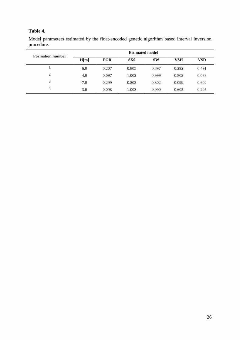
The inversion results can be found in Table 4. The estimated formation thicknesses were
accurate to the fourth decimal place (H1=6.0000m, H2=4.0000m, H3=7.0000m, H4=3.0000m)
despite the data noise. Petrophysical parameters were estimated close to their values in the
target model (see Table 2). In Fig. 4, the logs of the estimated petrophysical parameters and
the calculated formation boundary coordinates (Z1, Z2, Z3) can be seen. The overdetermination
ratio of the inverse problem decreased marginally by treating formation thicknesses as
inversion unknowns, but it did not caused a detectable quality loss in the overall estimation.
The CPU time was 6 minutes by using a quad-core processor based workstation.
4.2. Field case
We tested the inversion method using real well logs originated from a Hungarian
hydrocarbon exploratory well. Nine homogeneous formations were assumed by preliminary
study of well logs for the interval of 35m in length. The well logs in the interval of 1865-
1900m can be seen in Fig. 5. We processed SP, GR, CN, DEN, ATL, RS, RD data in Well-1
(see Table 1), where the sampling interval of well logging was 0.1m. The sequence consisted
of gas-bearing shaly sand formations and interbedded shale layers. The presence of gas was
confirmed by the indication on the neutron porosity vs. density crossplot and the separation of
CN and DEN logs. The cause of separation is that in gas-bearing zones significantly lower
neutron porosity and bulk density values are observed than in the water-bearing sand or shale
environment (Serra, 1984). In Fig. 5 neutron and density scales are drawn in a reversed
position, which enables the detection of gas-bearing zones easily. This overlay method is
frequently used in quick look interpretation of nuclear logs (Asquith and Krygowski, 2004).
We used well-logging data for computing petrophysical parameters and formation
thicknesses by the interval inversion method. For forward modeling, the response equations
Page 18
18
defined in eqs. (1)-(7) were used. The genetic algorithm based interval inversion procedure
required 104
iteration steps for updating 30 models at the same time by using real valued
genetic operations (see Section 2.3.2). We set the search space by using a priori petrophysical
information about the area (see Table 5). In the first 20 iteration steps the formation
thicknesses were found, after which the petrophysical parameters also attained to their
optimum. The development of convergence was smooth and steady (see Fig. 6). The average
data distance of the solution was 7.65%, which was caused by the data noise and the
application of the homogeneous model approximation by using eq. (27).
The logs of estimated petrophysical parameters can be seen in Fig. 7. We derived absolute
permeability for each formation by using eq. (14). The movable and irreducible gas saturation
was computed by substituting water saturation estimated by inversion into eqs. (12)-(13). The
result of the novel determination of 9 formation thicknesses is represented on the first track.
The depth scale contains the estimated formation boundary coordinates, which can be
compared directly with the gamma ray log. The method distinguished well the permeable and
non-permeable intervals within the hydrocarbon zone and gave rock interfaces back at the
same places as they were inferred from the GR log. Computations were taken only 2 minutes.
Discussion
The purport of the interval inversion method is the use of series expansion for defining
homogeneous intervals. The homogeneous model can be extended to inhomogeneous
petrophysical parameter distribution, too. Using polynomials for basis functions sets new
perspectives for improving the quality of the interval inversion results. On the other hand, the
inversion method can be further developed also for multi-well applications by using basis
functions depending on more spatial coordinates. In that case, the formation boundaries can
be described by appropriate 2D or 3D functions and the morphology and the volume of the
Page 19
19
hydrocarbon reservoir can be determined. These possibilities are based on the large extent of
overdetermination, which is not reduced significantly by introducing some additional
unknowns into the inverse problem. In this study, we presented layer boundary coordinates as
inversion parameters that cannot be determined by local inversion or another automatic way.
By means of the interval inversion method, the formation boundaries can be computed from a
more objective source than is done routinely today. Additionally, instead of local information
the method gives an estimate for petrophysical properties of layers, which can be used directly
in the classification of hydrocarbon zones.
Conclusions
An automated inversion procedure was shown for determination of formation thicknesses
based on well-logging data. The interval inversion method gives an estimate for the reservoir
parameters for an arbitrary depth interval and formation boundary coordinates in a joint
inversion procedure. The only necessary a priori knowledge is the number of formations in
the interval, which can probably be automated, e.g. by cluster analysis of well-logging data.
Based on the interval inversion results, we can provide the user permeability and hydrocarbon
saturation for the processed interval, which underlie the classification of hydrocarbon
reservoirs. Beside accurate and reliable parameter estimation, the CPU time of the inversion
procedure is not too much for a global optimization, which can be reduced further by applying
a more powerful machine. This advantage comes from the relatively simple structure of probe
response equations and a fast forward modeling procedure. In conclusion, the interval
inversion method can be applied well to extract detailed petrophysical information from well-
logging data, which speed up the analysis process of reservoir properties and layering
characteristics related to hydrocarbon exploration.
Page 20
20
Acknowledgement
The described work was carried out as part of the TÁMOP-4.2.1.B-10/2/KONV-2010-
0001 project in the framework of the New Hungarian Development Plan. The realization of
this project is supported by the European Union, co-financed by the European Social Fund.
The authors are grateful for the support of the Hungarian Oil and Gas Company for proving
field data for the research. The authors are also grateful to an unknown referee for the
suggestions, which appreciably improved the quality of the paper.
References
Alberty, M., Hashmy, K., 1984. Application of ULTRA to log analysis. SPWLA Symposium
Transactions, Paper Z, 1-17.
Asquith, G., Krygowski, D., 2004. Basic well log analysis. Second Edition. AAPG Methods
in Exploration Series 16. American Association of Petroleum Geologists, Tulsa.
Ball, S.M., Chace, D.M., Fertl, W.H., 1987. The Well Data System (WDS): An advanced
formation evaluation concept in a microcomputer environment. Proc. SPE Eastern Regional
Meeting, Paper 17034, 61-85.
Dobróka, M., Gyulai, Á., Ormos, T., Csókás, J., Dresen, L., 1991. Joint inversion of seismic
and geoelectric data recorded in an underground coal mine. Geophysical Prospecting 39, 643-
655.
Dobróka, M., 1993. The establishment of joint inversion algorithms in the well-logging
interpretation (in Hungarian). Scientific Report for the Hungarian Oil and Gas Company.
University of Miskolc.
Dobróka, M., Szabó, N.P., 2002. The MSA inversion of openhole well log data. Publications
of Ufa State Petroleum Technological University and University of Miskolc 2, 27-38.
Page 21
21
Dobróka, M., Szabó, N.P., 2005. Combined global/linear inversion of well-logging data in
layer-wise homogeneous and inhomogeneous media. Acta Geodaetica et Geophysica
Hungarica 40, 203-214.
Dobróka, M., Kiss, B., Szabó, N., Tóth, J., Ormos, T., 2007. Determination of cementation
exponent using an interval inversion method. EAGE Extended Abstracts, Paper 092, 1-4.
Dobróka, M., Szabó, N., Ormos, T., Kiss, B., Tóth, J., Szabó, I., 2008. Interval inversion of
borehole geophysical data for surveying multimineral rocks. Proc. European Meeting of
Environmental and Engineering Geophysics, Paper 11, 1-4.
Dobróka, M., Szabó, N. P., 2011. Interval inversion of well-logging data for objective
determination of textural parameters. Acta Geophysica, 59, 907-934.
Goswami, J.C., Mydur, R., Wu, P., Heliot, D., 2004. A robust technique for well-log data
inversion. IEEE Transactions on Antennas and Propagation 52, 717-724.
Lynch, E.J., 1962. Formation evaluation. Harper and Row, New York.
Mayer, C., Sibbit, A., 1980. GLOBAL, a new approach to computer-processed log
interpretation. Proc. SPE Annual Fall Technical Conference and Exhibition, Paper 9341, 1-14.
Michalewicz, Z., 1992. Genetic Algorithms + Data Structures = Evolution Programs. Third,
revised and extended version. Springer-Verlag, New York.
Poupon, A., Leveaux, J., 1971. Evaluation of water saturation in shaly formations. The Log
Analyst 12, 3-8.
Serra, O., 1984. Fundamentals of well-log interpretation. Elsevier, Amsterdam.
Szabó, N.P., 2004. Global inversion of well log data. Geophysical Transactions 44, 313-329.
Szucs, P., Civan, F., 1996. Multi-layer well log interpretation using the simulated annealing
method. Journal of Petroleum Science and Engineering 14, 209-220.
Tiab, D., Donaldson, E.C., 2004. Petrophysics. Theory and practice of measuring reservoir
rock and fluid transport properties. Second Edition. Elsevier Inc., New York.
Page 22
22
Timur, A., 1968. An investigation of permeability, porosity and residual water saturation
relationships for sandstone reservoirs. The Log Analyst 9, 8-17.
Zhou, C., Gao, C., Jin, Z., Wu, X., 1992. A simulated annealing approach to constrained
nonlinear optimization of formation parameters in quantitative log evaluation. SPE Annual
Technical Conference and Exhibition, Paper 24723, 1-9.
Page 23
23
Tables
Table 1.
Well log types used in hydrocarbon exploration and their specification.
Code Symbol Name of well log Sensitive to Unit
SP SP spontaneous potential mV
GR GR natural gamma ray intensity API
K K potassium (spectral gamma ray intensity) per cent
U U uranium (spectral gamma ray intensity) lithology ppm
TH TH thorium (spectral gamma ray intensity) ppm
PE Pe photoelectric absorption index barn/electron
CAL d caliper inch
CN ΦN compensated neutron porosity porosity unit
DEN ρb density porosity g/cm3
AT ∆t acoustic travel time µs/m
RMLL
RS
Rmll
Rs
microlaterolog
shallow resistivity
saturation
ohmm
ohm
RD Rd deep resistivity ohm
Page 24
24
Table 2.
Parameters of known petrophysical model for the interval inversion procedure.
Formation number Target model
H[m] POR SX0 SW VSH VSD
1 6.0 0.20 0.80 0.40 0.30 0.50
2 4.0 0.10 1.00 1.00 0.80 0.10
3 7.0 0.30 0.80 0.30 0.10 0.60
4 3.0 0.10 1.00 1.00 0.60 0.30
Page 25
25
Table 3.
A priori defined limits of individuals for float-encoded genetic algorithm search used in
synthetic inversion experiment.
Model parameter Lower bound Upper bound
H [m] 0.1 10
POR 0 0.5
SX0 0 1.0
SW 0 1.0
VSH 0 1.0
VSD 0 1.0
Page 26
26
Table 4.
Model parameters estimated by the float-encoded genetic algorithm based interval inversion
procedure.
Formation number Estimated model
H[m] POR SX0 SW VSH VSD
1 6.0 0.207 0.805 0.397 0.292 0.491
2 4.0 0.097 1.002 0.999 0.802 0.088
3 7.0 0.299 0.802 0.302 0.099 0.602
4 3.0 0.098 1.003 0.999 0.605 0.295
Page 27
27
Table 5.
A priori defined limits of individuals for the float-encoded genetic algorithm used in field
study.
Model parameter Lower bound Upper bound
H [m] 0.1 10
POR 0 0.35
SX0 0.6 1.0
SW 0.2 1.0
VSH 0 1.0
VSD 0 1.0
Page 28
28
Figure captions
Figure 1. Synthetic well logs contaminated with 5% Gaussian noise. Notations are
spontaneous potential (SP), natural gamma-ray intensity (GR), density (DEN), neutron
porosity (CN), acoustic travel time (AT), shallow resistivity (RS) and deep resistivity (RD).
Figure 2. The convergence of the interval inversion procedure. The average data distance of
model populations vs. number of iteration (generation) steps (on the left) and the average
model distance vs. number of iteration (generation) steps (on the right) are plotted.
Figure 3. The variation of formation thicknesses during the interval inversion procedure. The
petrophysical model including the thickness values can be found in Table 2.
Figure 4. The result of the interval inversion procedure. Notations are porosity (POR), water
saturation of the invaded zone (SX0), water saturation of the undisturbed zone (SW), shale
volume (VSH) and volume of quartz (VSD). Estimated formation boundary coordinates Z1, Z2,
Z3 are represented on the track of porosity log.
Figure 5. Well logs measured in Well-1. On the first track, the spontaneous potential (SP),
natural gamma-ray (GR) and caliper (CAL) logs are plotted. On the resistivity track, the
microlaterolog (RMLL), shallow- (RS) and deep resistivity (RD) logs can be seen. On the last
track, the neutron porosity (CNL), acoustic travel time (ATL) and density (DEN) logs are
represented. The separation of density and neutron porosity logs indicates the presence of
hydrocarbon (see shaded section).
Figure 6. The convergence of the interval inversion procedure. The average data distance of
model populations vs. number of iteration (generation) step is plotted.
Figure 7. The result of the interval inversion procedure. On the first track, the natural gamma-
ray (GR) log and the automatically estimated values of layer-boundary coordinates are
represented. On the second track, permeability (PERM) derived from inversion results can be
seen. On the third track density and neutron porosity logs are shown. On the fourth track,
movable and irreducible hydrocarbon saturation as derived logs can be found. On the last
track, shale content (VSH), porosity and specific volume of sand can be seen.
Page 29
29
Figures
Fig. 1


![Q analysis on reflection seismic data - Imperial College … · · 2016-04-21Q analysis on reflection seismic data ... Introduction [2] ... Interval-Q Calculation by Inversion [20]TwoQ-analysis](https://static.documents.pub/doc/80x56/5af38bc17f8b9a95468cb548/q-analysis-on-reflection-seismic-data-imperial-college-analysis-on-reflection.jpg)


