Introducing water by river basin into the GTAP-BIO model: GTAP-BIO-W By Farzad Taheripour** Thomas W. Hertel Jing Liu GTAP Working Paper No. 77 2013 **Corresponding Author: Farzad Taheripour, Department of Agricultural Economics, Purdue University, 403 West State St., West Lafayette, IN 47907-2056, Phone: 765-494-4612, E-mail: [email protected]. Farzad Taheripour is Research Assistant Professor, Thomas W. Hertel is Distinguished Professor, and Jing Liu is Ph.D. student in the Department of Agricultural Economics at Purdue University.
Transcript
Introducing water by river basin into the GTAP-BIO model:
GTAP-BIO-W
By
Farzad Taheripour**
Thomas W. Hertel Jing Liu
GTAP Working Paper No. 77
2013
**Corresponding Author: Farzad Taheripour, Department of Agricultural Economics, Purdue University, 403 West State St., West Lafayette, IN 47907-2056, Phone: 765-494-4612, E-mail: [email protected]. Farzad Taheripour is Research Assistant Professor, Thomas W. Hertel is Distinguished Professor, and Jing Liu is Ph.D. student in the Department of Agricultural Economics at Purdue University.
2
Introducing Water by river basin into the GTAP Model: GTAP-BIO-W
Farzad Taheripour, Thomas W. Hertel, and Jing Liu Abstract
This paper introduces water into the GTAP modeling framework at a river basin level. The new model: 1) distinguishes between irrigated and rainfed agriculture using different production functions; 2) takes into account heterogeneity in land quality across agro-ecological zones; 3) traces supply of water at the river basin level within each country/region; 4) fully captures competition for land among crop, livestock and forestry industries; 5) and, most importantly, offers the potential to extend the competition for managed water among agricultural and non-agricultural activities.
Key words: Water, Irrigation, Computable general equilibrium, River basin, Land, Agro ecological zone. JEL classification: C68, Q15, Q24, Q25.
3
1. Introduction
GTAP is a global Computable General Equilibrium (CGE) model which traces production, consumption, and trade of a wide range of goods and service across the world while takes into account market clearing conditions and resource constraints. In recent years, the land-use augmented versions of this model (GTAP-AEZ, GTAP-BIO-AEZ, GTAP-BIO-ADV) have been extensively used to address trade, development, energy, environment, climate, welfare, poverty, land, agriculture, and food security issues and their interactions with land resources.
While the GTAP model has been frequently used to address the land use related topics, only a few attempts have been made to extend its application in the areas of research on water. To the best of our knowledge so far only two major attempts have been made to introduce water into the GTAP modeling framework. In the first trial, Berrittella et al. (2007) have introduced managed water as an exogenous endowment into the GTAP standard model. Henceforth, we refer to this model as GTAP-W1. In this model crop and livestock industries only use water and the price of water is zero when there is no water scarcity. However, if water is scarce, then the economic rents associated with water resources drive a wedge between the market and agent prices of each commodity. This model assumed no substitution between water and other primary intermediate inputs.
In the second trial Calzadilla et al. (2010) have used a different approach to introduce managed water as an exogenous endowment into the GTAP standard model. Henceforth we refer to the model developed by these authors as GTAP-W2. In this model only crop industries use water. This model divided the standard value added of cropland into three categories of rainfed land, irrigated land, and irrigation. The first two components represent value added of rainfed and irrigated croplands, respectively. The latter component (irrigation) shows payments for water and has been calculated from the difference between the irrigated and rainfed yields.
Unlike the first model, the GTAP-W2 allows substitution between water and other primary inputs. It first combines water (irrigation) and irrigated land with a non-zero elasticity of substitution. Then it combines the composite of land-water with other primary inputs including rainfed land, labor, and capital with a non-zero elasticity of substitution in the value added nests of the production functions of crop industries. Thus there are two margins along which irrigation water can be conserved: by using more irrigated land, and by using more sophisticated irrigation techniques (labor and capital substitution) or by using more rainfed land. The former margin does not appear very realistic, while the latter component seems to mix a variety of important substitution possibilities.
Perhaps most importantly, these earlier approaches to incorporating irrigation into the GTAP model do not distinguish between the irrigated and rainfed production functions. GTAP-W1 only included water as an aggregated input into the national production functions of crop and livestock industries which subsequently produced output from both rainfed and irrigated farming. GTAP-W2 distinguishes between the irrigated land and rainfed land inputs, but does not differentiate between the irrigated and rainfed production functions themselves. This obscures the fact that rainfed and irrigated crop producers may behave differently in response to economic and climate shocks. On the other hand, the climate variables may affect the rainfed and irrigated crops in different ways. Indeed, in the case of extreme water scarcity, irrigation in a given region may
4
be eliminated altogether. Hence, it is important to define separate production functions for rainfed and irrigated crops to capture these responses and impacts more accurately.
In addition to the first limitation, these pioneering modeling frameworks ignored the fact that the quality of land varies significantly within the boundaries of a country/region and that water scarcity may vary across River Basins (RBs) of a country/region. Within the border of a country/region productivity of land varies across Agro Ecological Zones (AEZs) and intensity of water scarcity alters from one basin to another one. Finally, in these two models crop and livestock industries are the only active industries in the market for land. Therefore, these models do not fully capture the competition for land among crop, livestock, and forestry industries.
In this paper we develop a new modeling framework which: 1) distinguishes between irrigated and rainfed agriculture using different production functions; 2) takes into account heterogeneity in land quality across AEZs; 3) traces supply of water at the RB level within each country/region; 4) fully captures competition for land among crop, livestock and forestry industries; 5) and, most importantly, offers the potential to extend the competition for managed water among agricultural and non-agricultural activities. The rest of this paper describes the configurations of the new modeling framework and its data base.
2. Modeling Framework
To build the new model we begin with the model developed by Taheripour, Hertel, and Liu (2013: Henceforth THL). These authors have extended the GTAP-BIO1 model by splitting the crop industries into irrigated and rainfed activities. Their model considers water as an implicit input imbedded in the irrigated land and traces demand for, and supply of, land by AEZ in each region, while defines distinct production functions for irrigated and rainfed crops. The GTAP-BIO model fully captures the competition for land among crop, livestock and forestry industries in each AEZ. In this paper, we extend this earlier model by introducing water as an explicit input into irrigated crop production.
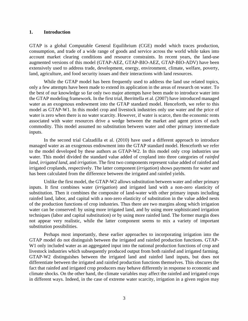
The structure of the new model (henceforth: GTAP-BIO-W) is presented in Figure 1. In this model there is a national competition among industries for labor, capital, and resources other than land and water. Water resources are available at a RB level, each country may have several RBs, and a RB may serve several AEZs. Supply of managed water in each RB is exogenously specified and agricultural and non-agricultural industries compete for managed water at the basin level. Water does not move across RBs but it can move across AEZs within a given basin. Following the earlier versions of the GTAP-BIO model, the new model also considers accessible land as an endowment with fixed supply at the AEZ level by region. The accessible land is divided into three groups of pasture, cropland, and forest. The crop, livestock, and forestry industries compete for land and crop industries compete for cropland. Irrigated crops use irrigated land and rainfed crops use rainfed land. Land can move from rainfed to irrigated agriculture and vice versa, if biophysical and economic factors allow such a conversion. At the national level, the irrigated and rainfed
1 This model is an advanced and improved version of the GTAP-E model which has been designed and frequently
used to examine the economic and environmental consequences of biofuel production and policies. Examples are: Hertel et al. (2010), Taheripour et al. (2010), Taheripour et al. (2011), Beckman et al. (2011), Diffenbaugh (2012), and Taheripour and Tyner (2013).
5
farmers supply a homogenous crop (but region-specific) product to domestic and foreign consumers.
Figure 1. Structure of the GTAP-BIO-W model
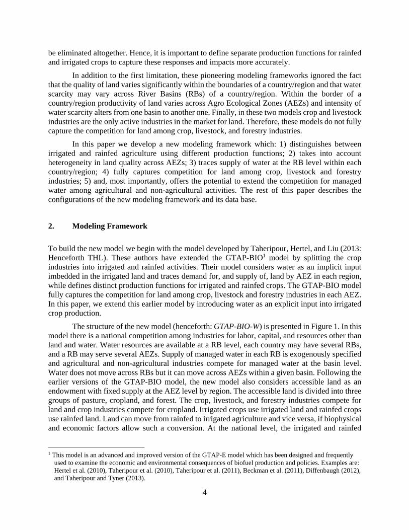
To implement the new modeling structure, each country/region is divided into several RBs (currently constrained to be a maximum 20 RB’s per region) and each RB serves several AEZs (maximum 18). Hence, the value added nests of the irrigated crop production functions are modified to trace demands for water and land at the RB-AEZ level, as shown in Figure 2. At the very bottom level of the value added nest, water and land are combined to create a composite input. For a given RB, the mix of this composite is aggregated across AEZs within the RB, and subsequently across RBs to determine the national demand for the mix of water and land in irrigated crop production. This set up also traces the demands for water and land at the RB and AEZ levels, respectively. In this model, the substitution rate between water and land inputs can vary across regions, industries, RBs, AEZs. Land can also move between irrigated and rainfed cropping according to the transformation elasticity as specified in the model.
6
Figure 2. Demand structure for primary inputs
To implement this modeling structure we made major modifications in the GTAP TABLO code. In addition to extensive changes in the demand and supply functions and market clearing conditions, we included the following market clearing condition for water to determine the shadow price of water at the river basin level:
, ∗ ∑ , , ∑ ∑ , , , ∗ , , , (1)
In this equation indices of i, z, j, r stand for RB, AEZ, industry, and region, respectively. The variables qobasin and qfe show percentage changes in the supply of, and demand for, water. Finally, VOM and VFM represent the implied values of water and water used by industries. In this equation: ∑ , , ∑ ∑ , , , . The left hand side of this relationship represents implied value of water at the river basin level and the right hand side represents sum of values of water used by industries again at the river basin level. The river basin market clearing conditions for water determine the shadow price of water at the river basin level.
3. Data base
While the modeling framework developed in the previous section is very general and with minor modifications can handle competition for water among all water-using industries, in this section we assume that only irrigated crop industries compete for managed water. To build the new data base we begin with the data base developed by THL. This data base is a modified version of the
7
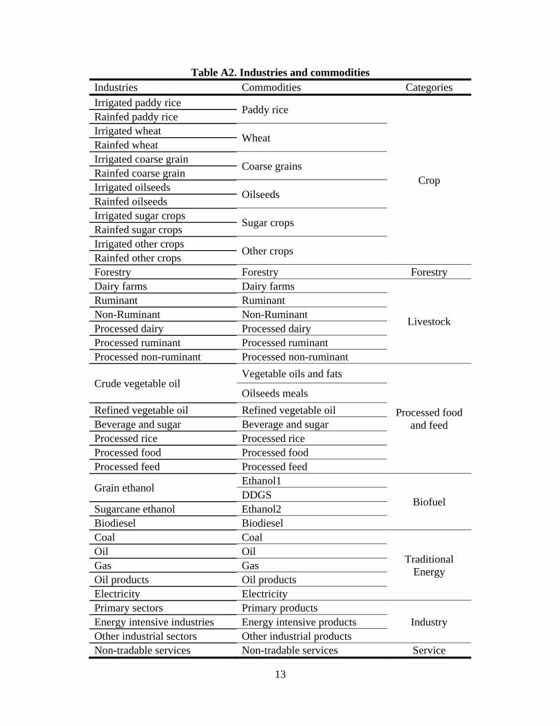
standard GTAP data base version 6 which represents production, consumption, and trade of a wide range of good and services, including biofuels and their by-products, at the global scale in 2001. This data base divided the world economy into 19 region, 37 industries, and 33 commodities as listed in Appendix A. We made several major modifications in this data base as explained in the following sections.
3.1. Modification in bio-physical data
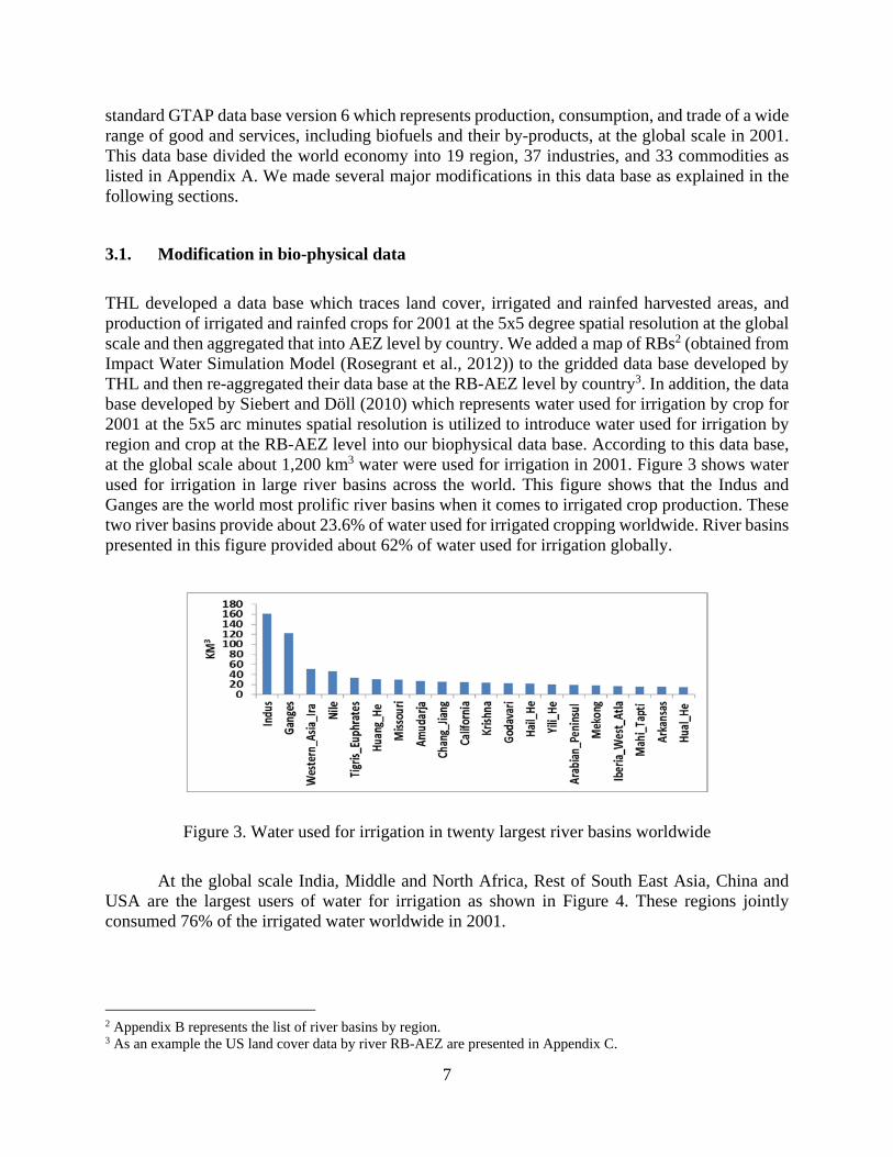
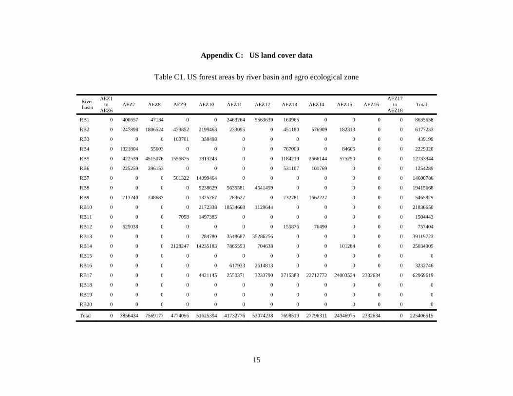
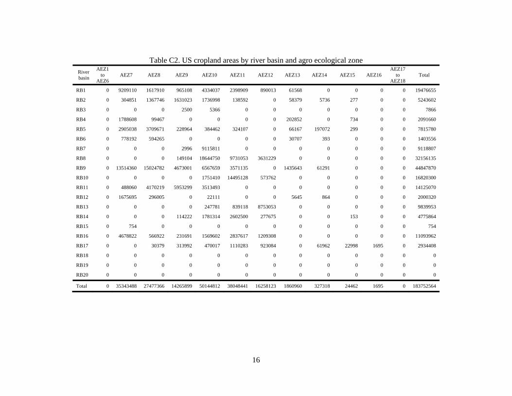
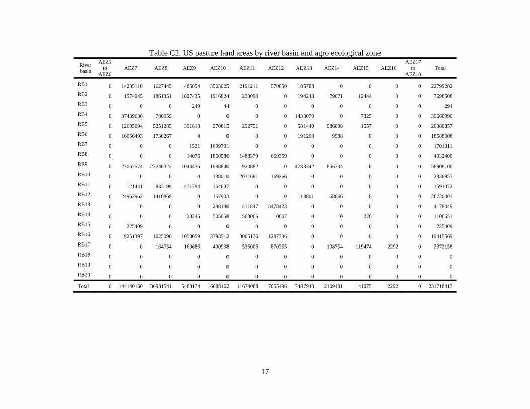
THL developed a data base which traces land cover, irrigated and rainfed harvested areas, and production of irrigated and rainfed crops for 2001 at the 5x5 degree spatial resolution at the global scale and then aggregated that into AEZ level by country. We added a map of RBs2 (obtained from Impact Water Simulation Model (Rosegrant et al., 2012)) to the gridded data base developed by THL and then re-aggregated their data base at the RB-AEZ level by country3. In addition, the data base developed by Siebert and Döll (2010) which represents water used for irrigation by crop for 2001 at the 5x5 arc minutes spatial resolution is utilized to introduce water used for irrigation by region and crop at the RB-AEZ level into our biophysical data base. According to this data base, at the global scale about 1,200 km3 water were used for irrigation in 2001. Figure 3 shows water used for irrigation in large river basins across the world. This figure shows that the Indus and Ganges are the world most prolific river basins when it comes to irrigated crop production. These two river basins provide about 23.6% of water used for irrigated cropping worldwide. River basins presented in this figure provided about 62% of water used for irrigation globally.
Figure 3. Water used for irrigation in twenty largest river basins worldwide
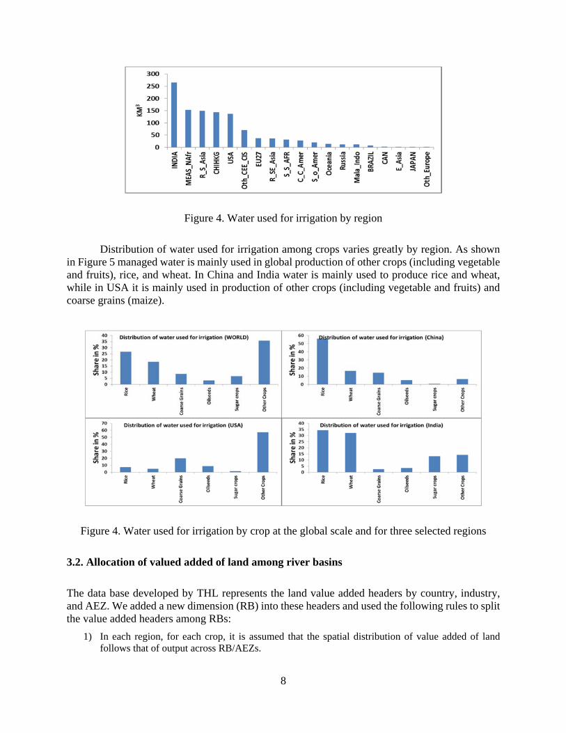
At the global scale India, Middle and North Africa, Rest of South East Asia, China and USA are the largest users of water for irrigation as shown in Figure 4. These regions jointly consumed 76% of the irrigated water worldwide in 2001.
2 Appendix B represents the list of river basins by region. 3 As an example the US land cover data by river RB-AEZ are presented in Appendix C.
8
Figure 4. Water used for irrigation by region
Distribution of water used for irrigation among crops varies greatly by region. As shown in Figure 5 managed water is mainly used in global production of other crops (including vegetable and fruits), rice, and wheat. In China and India water is mainly used to produce rice and wheat, while in USA it is mainly used in production of other crops (including vegetable and fruits) and coarse grains (maize).
Figure 4. Water used for irrigation by crop at the global scale and for three selected regions
3.2. Allocation of valued added of land among river basins
The data base developed by THL represents the land value added headers by country, industry, and AEZ. We added a new dimension (RB) into these headers and used the following rules to split the value added headers among RBs:
1) In each region, for each crop, it is assumed that the spatial distribution of value added of land follows that of output across RB/AEZs.
9
2) In each region for the forestry sector it is assumed that the spatial distribution of value added of land follows that of forest land across RB/AEZs.
3) In each region for each livestock industry is assumed that the spatial distribution of value added of land follows that of pasture land across RB/AEZs.
4) It is assumed that the rate of taxation (subsidy) on the land input does not vary across RB/AEZs.
3.3. Splitting value added of irrigated land between water and land
The value added of irrigated cropland presented in the data base developed by THL measures the value added of the mix of land-water. We denote this mix, valued at agent’s prices, by EFVA_LW(i,z,j,r). To split this mix between land (EVFA_L(i,z,j,r)) and water (EVFA_W(i,z,j,r)) the following formulas and steps are used:
Here EVFA and AREA represent land value added (in million dollar) and harvested area (in hectare). Of course for rainfed crops EFVA_LW(i,z,j,r)=EFVA_L(i,z,j,r), because they do not use managed water for irrigation.
2) The difference between the irrigated and rainfed rents is calculated for each crop:
, , , , , , , , , . (3)
3) It is assumed that the coefficient DIFF represents the implicit value of water per hectare of irrigated land. Hence the value added of water is calculated for each irrigated crop using the following formula:
_ , , , , , , ∗ , , , . (4)
4) Finally the value added of land is calculated for each irrigated crop using the following formula:
_ , , , _ , , , _ , , , (5)
5) The same process is followed to split the value added at market price as well.
3.4. Arrangement of value added headers in the final data base
The GTAP standard data base represents five primary inputs including: skilled labor, unskilled labor, capital, land, and resources and handles value added headers using the ENDW_COMM set with a vector with 5 rows. The GTAP-BIO model follows the same tradition but divides the land input into 18 AEZs. Hence in the GTAP-BIO model the ENDW_COMM set has 22 rows (including 4 non-land inputs and 18 AEZs). In the new model the endowment set has 724 rows. The first 18 rows represent land in RB1-AEZ1 to RB1-AEZ18; the second 18 rows represent land in RB2-AEZ1 to RB2-AEZ18; and so on. Hence, the rows 343 to 360 represent land in RB20-AEZ1 to RB20-AEZ18. The next 360 rows (i.e. rows 361 to 720) represent water following the same order used for land. Finally, the last four rows (i.e. rows 721 to 724) represent skilled labor, unskilled labor, capital, and resources.
10
4. Applications
The modeling framework developed in this paper provides a flexible tool that can be used to examine a wide variety of water related topics and issues. Two primary applications of this model are discussed in Liu et al. (2013) and Taheripour et al. (2013). The first application examines the consequences of water scarcity for the food security and trade of food and the second application studies consequences of water scarcity and climate change in the presence of biofuel production for rainfed and irrigated agriculture. More applications will be developed in future.
11
Resources Beckman J., Hertel T., Taheripour F., and Tyner W. (2012) “Structural Change in the Biofuels
Era,” European Review of Agricultural Economics, 39 (1): 137–156. Berrittella M., Hoekstra A., Rehdanz K., Roson R., Tol R. (2007) “The economic impact of
restricted water supply: A computable general equilibrium analysis,” Water Research, 41(8): 1799-1813.
Calzadilla A., Rehdanz K., and Tol, R. (2010) “The economic impact of more sustainable water use in agriculture: A computable general equilibrium analysis,” Journal of Hydrology, 384(3–4), 292–305.
Diffenbaugh N., Hertel T., Scherer M., Verma M. (2012) “Response of corn markets to climate volatility under alternative energy futures,” Nature Climate Change 2, 514–518.
Hertel T., Golub A., Jones A., O’Hare M., Pelvin R., Kammen D. (2010) “Effects of U.S. maize ethanol on global land use and greenhouse gas emissions: estimating market-mediated responses,” BioScience 60(3):223-231.
Liu J., Hertel T., Taheripour F., Zhu T., and Ringler C. (2013), “Water Scarcity and International Agricultural Trade,” presented at the 16th Annual Conference on Global Economic Analysis, “New Challenges for Global Trade in a Rapidly Changing World,” June 12-14, 2013, Shanghai, China.
Rosegrant M. & The IMPACT Development Team. (2012), “International model for policy analysis of agricultural commodities and trade (IMPACT) model description,” International Food Policy Research Institute, Washington, D.C. USA.
Siebert S., and Döll P. (2010) "Quantifying blue and green virtual water contents in global crop production as well as potential production losses without irrigation," Journal of Hydrology 384 (3): 198-217.
Taheripour F., Hertel T., Tyner W., Beckman J., and Birur D. (2010) “Biofuels and their by-products: global economic and environmental implications,” Biomass and Bioenergy 34(3): 278-289.
Taheripour F., Hertel T., Tyner W. (2011) “Implications of biofuels mandates for the global livestock industry: a computable general equilibrium analysis,” Agricultural Economics 42(3): 325-342.
Taheripour F., Hertel T., and Liu J. (2012) “The Role of Irrigation in Determining the Global Land Use Impacts of Biofuels,” Energy, Sustainability, and Society, 3(4): 1-18.
Taheripour F. and Tyner W. (2013) “Induced Land Use Emissions Due to First and Second Generation Biofuels and Uncertainty in Land Use Emissions Factors,” Economics Research International, Vol 2013, Article ID 315787: 1-12.
Taheripour F., Hertel T., and Liu J. (2013), “Water Reliability, Irrigation, Biofuel Production, Land Use Changes, and Trade Nexus,” at the 16th Annual Conference on Global Economic Analysis, “New Challenges for Global Trade in a Rapidly Changing World,” June 12-14, 2013, Shanghai, China.
12
Appendix A: Regional, industry, and commodity aggregation schedules
Table A1. Regional aggregation and members of each region
Region Description Corresponding Countries in GTAP
Oil Oil Gas Gas Oil products Oil products Electricity Electricity Primary sectors Primary products
Industry Energy intensive industries Energy intensive products Other industrial sectors Other industrial products Non-tradable services Non-tradable services Service
14
Appendix B: List of river basins by region
Table B1. Regions and their river basins USA EU27 BRAZIL CAN JAPAN CHIHKG INDIA Central America South America