Introduction to General Relativity and Gravitational …...Introduction to General Relativity and...

Introduction to General Relativity andGravitational Waves

Patrick J. Sutton

Cardiff University

International School of Physics “Enrico Fermi”Varenna, 2017/07/03-04

LIGO-G1701235-v1 Sutton GR and GWs

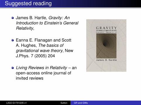
Suggested reading

James B. Hartle, Gravity: AnIntroduction to Einstein’s GeneralRelativity,

Eanna E. Flanagan and ScottA. Hughes, The basics ofgravitational wave theory, NewJ.Phys. 7 (2005) 204

Living Reviews in Relativity – anopen-access online journal ofinvited reviews


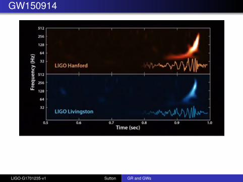
GW150914


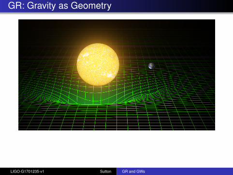
GR: Gravity as Geometry


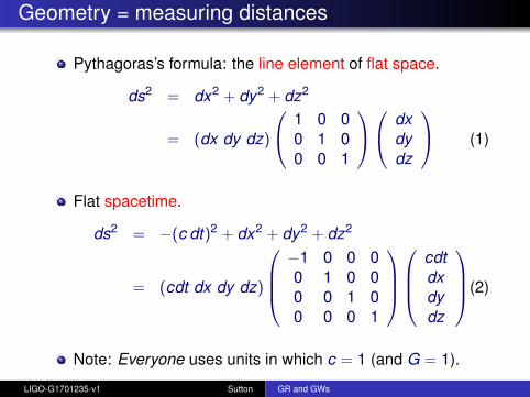
Geometry = measuring distances

Pythagoras’s formula: the line element of flat space.

ds2 = dx2 + dy2 + dz2

= (dx dy dz)

1 0 00 1 00 0 1

dxdydz

(1)

Flat spacetime.

ds2 = −(c dt)2 + dx2 + dy2 + dz2

= (cdt dx dy dz)

−1 0 0 00 1 0 00 0 1 00 0 0 1

cdtdxdydz

(2)

Note: Everyone uses units in which c = 1 (and G = 1).


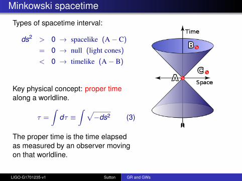
Minkowski spacetime

Types of spacetime interval:

ds2 > 0 → spacelike (A− C)

= 0 → null (light cones)

< 0 → timelike (A− B)

Key physical concept: proper timealong a worldline.

τ =

∫dτ ≡

∫ √−ds2 (3)

The proper time is the time elapsedas measured by an observer movingon that worldline.


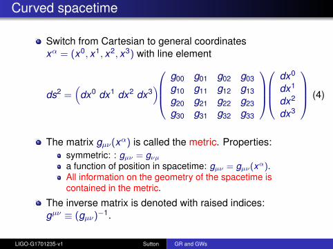
Curved spacetime

Switch from Cartesian to general coordinatesxα = (x0, x1, x2, x3) with line element

ds2 =(

dx0 dx1 dx2 dx3)

g00 g01 g02 g03g10 g11 g12 g13g20 g21 g22 g23g30 g31 g32 g33

dx0

dx1

dx2

dx3

(4)

The matrix gµν(xα) is called the metric. Properties:symmetric: : gµν = gνµ

a function of position in spacetime: gµν = gµν(xα).All information on the geometry of the spacetime iscontained in the metric.

The inverse matrix is denoted with raised indices:gµν ≡ (gµν)−1.


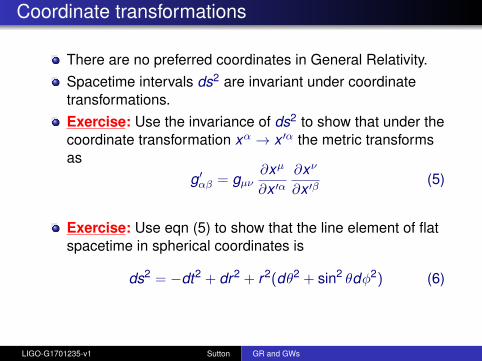
Coordinate transformations

There are no preferred coordinates in General Relativity.Spacetime intervals ds2 are invariant under coordinatetransformations.Exercise: Use the invariance of ds2 to show that under thecoordinate transformation xα → x ′α the metric transformsas

g′αβ = gµν∂xµ

∂x ′α∂xν

∂x ′β(5)

Exercise: Use eqn (5) to show that the line element of flatspacetime in spherical coordinates is

ds2 = −dt2 + dr2 + r2(dθ2 + sin2 θdφ2) (6)


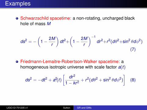
Examples

Schwarzschild spacetime: a non-rotating, uncharged blackhole of mass M

ds2 = −(

1− 2Mr

)dt2+

(1− 2M

r

)−1

dr2+r2(dθ2+sin2 θdφ2)

(7)

Friedmann-Lemaitre-Robertson-Walker spacetime: ahomogeneous isotropic universe with scale factor a(t)

ds2 = −dt2 + a2(t)[

dr2

1− kr2 + r2(dθ2 + sin2 θdφ2)

](8)


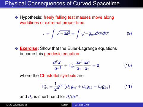
Physical Consequences of Curved Spacetime

Hypothesis: freely falling test masses move alongworldlines of extremal proper time.

τ =

∫ √−ds2 =

∫ √−gµνdxµdxν (9)

Exercise: Show that the Euler-Lagrange equationsbecome this geodesic equation:

d2xα

dτ2 + Γαβγdxβ

dτdxγ

dτ= 0 (10)

where the Christoffel symbols are

Γαβγ =12

gαδ (∂βgγδ + ∂γgδβ − ∂δgβγ) (11)

and ∂α is short-hand for ∂/∂xα.


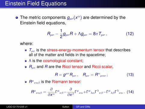
Einstein Field Equations

The metric components gµν(xα) are determined by theEinstein field equations,

Rµν −12

gµνR + Λgµν = 8πTµν , (12)

where:Tµν is the stress-energy-momentum tensor that describesall of the matter and fields in the spacetime;Λ is the cosmological constant;Rµν and R are the Ricci tensor and Ricci scalar,

R = gµνRµν , Rµν = Rαµαν ; (13)

Rµναβ is the Riemann tensor:

Rµναβ =

∂

∂xαΓµ

νβ−∂

∂xβΓµ

να+ΓµλαΓλ

νβ−ΓµλβΓλ

να . (14)


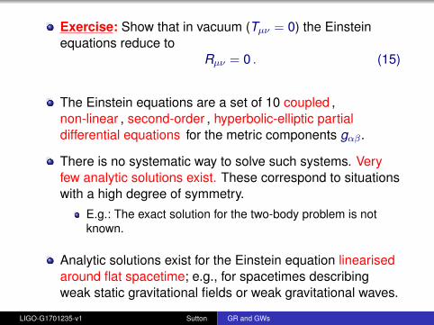
Exercise: Show that in vacuum (Tµν = 0) the Einsteinequations reduce to

Rµν = 0 . (15)

The Einstein equations are a set of 10 coupled ,non-linear , second-order , hyperbolic-elliptic partialdifferential equations for the metric components gαβ.

There is no systematic way to solve such systems. Veryfew analytic solutions exist. These correspond to situationswith a high degree of symmetry.

E.g.: The exact solution for the two-body problem is notknown.

Analytic solutions exist for the Einstein equation linearisedaround flat spacetime; e.g., for spacetimes describingweak static gravitational fields or weak gravitational waves.


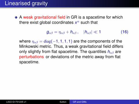
Linearised gravity

A weak gravitational field in GR is a spacetime for whichthere exist global coordinates xα such that

gαβ = ηαβ + hαβ , |hαβ| 1 (16)

where ηαβ = diag(−1,1,1,1) are the components of theMinkowski metric. Thus, a weak gravitational field differsonly slightly from flat spacetime. The quantities hαβ areperturbations or deviations of the metric away from flatspacetime.


A word about coordinate transformations:

It is always possible to find coordinates for which the abovedecomposition is not valid—e.g., flat spacetime inspherical polar coordinates does not satisfy (16), eventhough the gravitational field is identically zero!

The set of coordinates xα in which (16) holds is notunique. It is possible to make an infinitesimal coordinatetransformation xα → x ′α for which the decomposition withrespect to the new set of coordinates still holds.

We’ll often refer to these infinitesimal coordinatetransformations as gauge transformations.


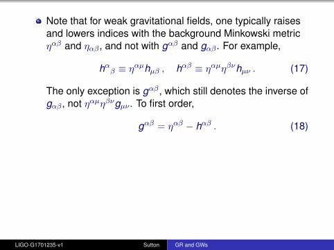
Note that for weak gravitational fields, one typically raisesand lowers indices with the background Minkowski metricηαβ and ηαβ, and not with gαβ and gαβ. For example,

hαβ ≡ ηαµhµβ , hαβ ≡ ηαµηβνhµν . (17)

The only exception is gαβ, which still denotes the inverse ofgαβ, not ηαµηβνgµν . To first order,

gαβ = ηαβ − hαβ . (18)


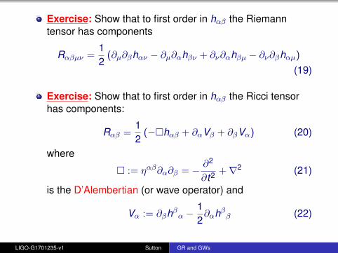
Exercise: Show that to first order in hαβ the Riemanntensor has components

Rαβµν =12

(∂µ∂βhαν − ∂µ∂αhβν + ∂ν∂αhβµ − ∂ν∂βhαµ)

(19)

Exercise: Show that to first order in hαβ the Ricci tensorhas components:

Rαβ =12

(−hαβ + ∂αVβ + ∂βVα) (20)

where

:= ηαβ∂α∂β = − ∂2

∂t2 +∇2 (21)

is the D’Alembertian (or wave operator) and

Vα := ∂βhβα −12∂αhββ (22)


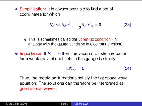
Simplification: It is always possible to find a set ofcoordinates for which

Vα := ∂βhβα −12∂αhββ = 0 (23)

This is sometimes called the Loren(t)z condition (inanalogy with the gauge condition in electromagnetism).

Importance: If Vα = 0 then the vacuum Einstein equationfor a weak gravitational field in this gauge is simply

hαβ = 0 (24)

Thus, the metric perturbations satisfy the flat space waveequation. The solutions can therefore be interpreted asgravitational waves.


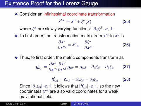
Existence Proof for the Lorenz Gauge

Consider an infinitesimal coordinate transformation

x ′α := xα + ξα(x) (25)

where ξα are slowly varying functions: |∂αξβ| 1.

To first-order, the transformation matrix from x ′α to xµ is∂xµ

∂x ′α= δµα −

∂ξµ

∂xα(26)

Thus, to first order, the metric components transform as

g′αβ =∂xµ

∂x ′α∂xν

∂x ′βgµν = gαβ − ∂αξβ − ∂βξα (27)

h′αβ = hαβ − ∂αξβ − ∂βξα (28)

Since |∂αξβ| 1, it follows that |h′αβ| 1, so the newcoordinates x ′α are also valid coordinates for a weakgravitational field.


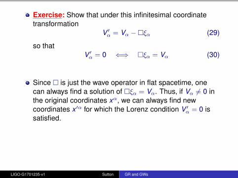
Exercise: Show that under this infinitesimal coordinatetransformation

V ′α = Vα −ξα (29)

so thatV ′α = 0 ⇐⇒ ξα = Vα (30)

Since is just the wave operator in flat spacetime, onecan always find a solution of ξα = Vα. Thus, if Vα 6= 0 inthe original coordinates xα, we can always find newcoordinates x ′α for which the Lorenz condition V ′α = 0 issatisfied.


Exercise: Show that under an infinitesimal coordinatetransformation the components of the Riemann tensorRµανβ given by eqn. (19) are unchanged to first-order.

This shows that the curvature of a weak-field spacetime,and so any physical predictions such as geodesicdeviation, are unchanged to first-order by an infinitesimalcoordinate transformation.


Solving the Wave Equation

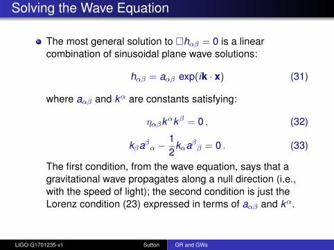
The most general solution to hαβ = 0 is a linearcombination of sinusoidal plane wave solutions:

hαβ = aαβ exp(ik · x) (31)

where aαβ and kα are constants satisfying:

ηαβkαkβ = 0 , (32)

kβaβα −12

kαaββ = 0 . (33)

The first condition, from the wave equation, says that agravitational wave propagates along a null direction (i.e.,with the speed of light); the second condition is just theLorenz condition (23) expressed in terms of aαβ and kα.


Transverse traceless gauge

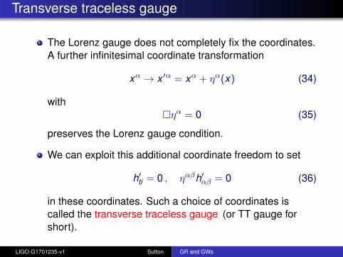
The Lorenz gauge does not completely fix the coordinates.A further infinitesimal coordinate transformation

xα → x ′α = xα + ηα(x) (34)

withηα = 0 (35)

preserves the Lorenz gauge condition.

We can exploit this additional coordinate freedom to set

h′ti = 0 , ηαβh′αβ = 0 (36)

in these coordinates. Such a choice of coordinates iscalled the transverse traceless gauge (or TT gauge forshort).


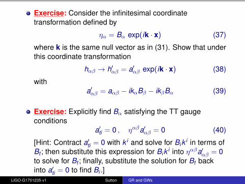
Exercise: Consider the infinitesimal coordinatetransformation defined by

ηα = Bα exp(ik · x) (37)

where k is the same null vector as in (31). Show that underthis coordinate transformation

hαβ → h′αβ = a′αβ exp(ik · x) (38)

witha′αβ = aαβ − ikαBβ − ikβBα (39)

Exercise: Explicitly find Bα satisfying the TT gaugeconditions

a′ti = 0 , ηαβa′αβ = 0 (40)

[Hint: Contract a′ti = 0 with k i and solve for Bik i in terms ofBt ; then substitute this expression for Bik i into ηαβa′αβ = 0to solve for Bt ; finally, substitute the solution for Bt backinto a′ti = 0 to find Bi .]


In the TT gauge, the Lorenz condition eqn. (23) reduces to∂βhβα = 0.Thus, in the TT gauge there are 8 conditions on the 10independent components of hαβ:

hti = 0 , ηαβhαβ = 0 , ∂βhβα = 0 (41)

This leaves only 2 independent components of hαβ.In terms of aαβ and kα, we have

ati = 0 , ηαβaαβ = 0 , kβaβα = 0 (42)

The remaining two independent components of aαβcorrespond to the two independent polarisation states of agravitational wave, typically denoted h+ and h×.


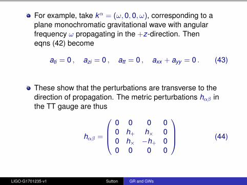
For example, take kα = (ω,0,0, ω), corresponding to aplane monochromatic gravitational wave with angularfrequency ω propagating in the +z-direction. Theneqns (42) become

ati = 0 , azi = 0 , att = 0 , axx + ayy = 0 . (43)

These show that the perturbations are transverse to thedirection of propagation. The metric perturbations hαβ inthe TT gauge are thus

hαβ =

0 0 0 00 h+ h× 00 h× −h+ 00 0 0 0

(44)


The corresponding line element is

ds2 = −dt2 + (1 + h+) dx2 + (1−h+) dy2 + 2h× dx dy + dz2

(45)

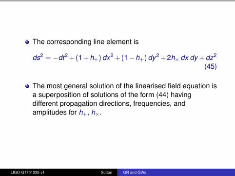
The most general solution of the linearised field equation isa superposition of solutions of the form (44) havingdifferent propagation directions, frequencies, andamplitudes for h+, h×.


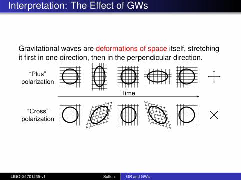
Interpretation: The Effect of GWs

Gravitational waves are deformations of space itself, stretchingit first in one direction, then in the perpendicular direction.

6

Gravitational Wave Basics

A consequence of Einstein’s general theory of relativity

Emitted by a massive object, or group of objects,

whose shape or orientation changes rapidly with time

Waves travel away from the source at the speed of light

Waves deform space itself, stretching it first in one direction, then

in the perpendicular direction

Time

“Plus”

polarization

“Cross”

polarization


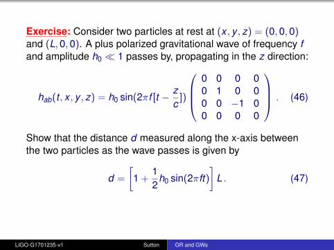
Exercise: Consider two particles at rest at (x , y , z) = (0,0,0)and (L,0,0). A plus polarized gravitational wave of frequency fand amplitude h0 1 passes by, propagating in the z direction:

hab(t , x , y , z) = h0 sin(2πf [t − zc

])

0 0 0 00 1 0 00 0 −1 00 0 0 0

. (46)

Show that the distance d measured along the x-axis betweenthe two particles as the wave passes is given by

d =

[1 +

12

h0 sin(2πft)]

L . (47)


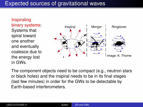
Expected sources of gravitational waves

Inspiralingbinary systems:Systems thatspiral towardone anotherand eventuallycoalesce due tothe energy lostin GWs.

11

Sources of GWs

Supernovae, Gamma-ray Bursts (GRBs) - short bursts of radiation

Deformed pulsars - steady sine-wave signal

Inspiraling binaries (neutron-star or black-hole) - chirps

Big Bang - stochastic (random) GW radiation background - like CMB

image: K. ThorneWMAP 2003 data

SN 1987A GRB / accreting BH

The component objects need to be compact (e.g., neutron starsor black holes) and the inspiral needs to be in its final stages(last few minutes) in order for the GWs to be detectable byEarth-based interferometers.


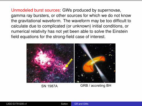
Unmodeled burst sources: GWs produced by supernovae,gamma ray bursters, or other sources for which we do not knowthe gravitational waveform. The waveform may be too difficult tocalculate due to complicated (or unknown) initial conditions, ornumerical relativity has not yet been able to solve the Einsteinfield equations for the strong-field case of interest.

11

Sources of GWs







11

Sources of GWs








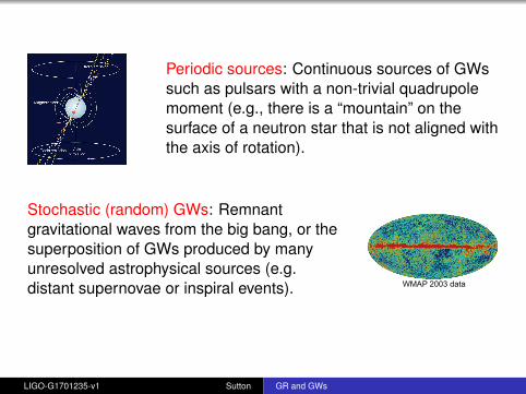
Periodic sources: Continuous sources of GWssuch as pulsars with a non-trivial quadrupolemoment (e.g., there is a “mountain” on thesurface of a neutron star that is not aligned withthe axis of rotation).

Stochastic (random) GWs: Remnantgravitational waves from the big bang, or thesuperposition of GWs produced by manyunresolved astrophysical sources (e.g.distant supernovae or inspiral events).

11

Sources of GWs








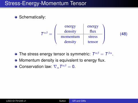
Stress-Energy-Momentum Tensor

Schematically:

Tαβ =

energydensity

energyflux

momentumdensity

stresstensor

(48)

The stress energy tensor is symmetric: Tαβ = T βα.Momentum density is equivalent to energy flux.Conservation law: ∇αTαβ = 0.


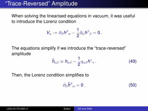
“Trace-Reversed” Amplitude

When solving the linearised equations in vacuum, it was usefulto introduce the Lorenz condition

Vα := ∂βhβα −12∂αhββ = 0 .

The equations simplify if we introduce the “trace-reversed”amplitude

hαβ ≡ hαβ −12ηαβhγγ . (49)

Then, the Lorenz condition simplifies to

∂βhβα = 0 . (50)


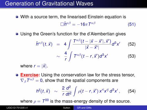
Generation of Gravitational Waves

With a source term, the linearised Einstein equation is

hαβ = −16πTαβ (51)

Using the Green’s function for the d’Alembertian gives

hαβ(t , ~x) = 4∫

Tαβ(t − |~x − ~x ′|, ~x ′)|~x − ~x ′|

d3x ′ (52)

∼ 4r

∫Tαβ(t − r , ~x ′)d3x ′ (53)

where r = |~x |.

Exercise: Using the conservation law for the stress tensor,∇βTαβ = 0, show that the spatial components are

hij(t , ~x) ∼ 2r

d2

dt2

∫ρ(t − r , ~x ′) x ′ix ′j d3x ′ , (54)

where ρ = T 00 is the mass-energy density of the source.LIGO-G1701235-v1 Sutton GR and GWs

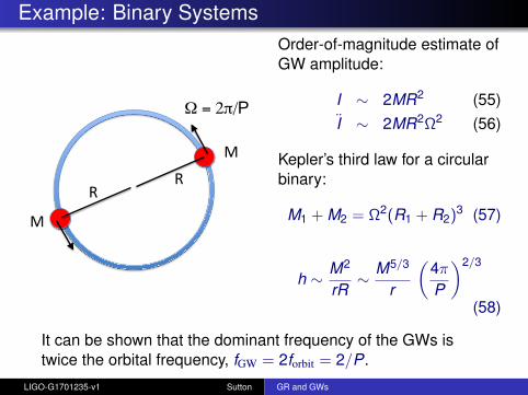
Example: Binary Systems

!"!"

#"

#"

! = 2"/P

Order-of-magnitude estimate ofGW amplitude:

I ∼ 2MR2 (55)I ∼ 2MR2Ω2 (56)

Kepler’s third law for a circularbinary:

M1 + M2 = Ω2(R1 + R2)3 (57)

h ∼ M2

rR∼ M5/3

r

(4πP

)2/3

(58)

It can be shown that the dominant frequency of the GWs istwice the orbital frequency, fGW = 2forbit = 2/P.


Exercise: For a neutron-star binary (M ' 1.4M) at 5 kpcwith P = 1 hr show that h ∼ 10−22.Exercise: For the same system with P = 0.02 s (givingfGW = 2forbit = 100 Hz, in the sensitive band of LIGO) showthat h ∼ 10−22 at a distance of 15 Mpc – approximately thedistance of the Virgo cluster of galaxies.Exercise: Show the orbital separation R ∼ 100 km whenP = 0.02 s. Thus, we can only hope to detect inspirals ofcompact binary systems (e.g., NS-NS, NS-BH, or BH-BH)with Earth-based interferometers like LIGO.


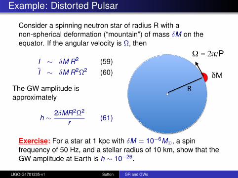
Example: Distorted Pulsar

Consider a spinning neutron star of radius R with anon-spherical deformation (“mountain”) of mass δM on theequator. If the angular velocity is Ω, then

I ∼ δM R2 (59)I ∼ δM R2Ω2 (60)

The GW amplitude isapproximately

h ∼ 2δMR2Ω2

r(61)

!"

!#"

" = 2#/P

Exercise: For a star at 1 kpc with δM = 10−6M, a spinfrequency of 50 Hz, and a stellar radius of 10 km, show that theGW amplitude at Earth is h ∼ 10−26.


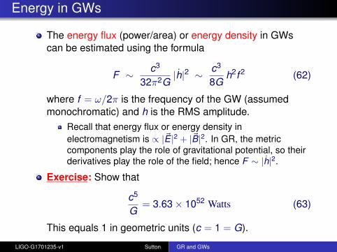
Energy in GWs

The energy flux (power/area) or energy density in GWscan be estimated using the formula

F ∼ c3

32π2G|h|2 ∼ c3

8Gh2f 2 (62)

where f = ω/2π is the frequency of the GW (assumedmonochromatic) and h is the RMS amplitude.

Recall that energy flux or energy density inelectromagnetism is ∝ |~E |2 + |~B|2. In GR, the metriccomponents play the role of gravitational potential, so theirderivatives play the role of the field; hence F ∼ |h|2.

Exercise: Show that

c5

G= 3.63× 1052 Watts (63)

This equals 1 in geometric units (c = 1 = G).


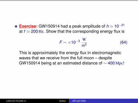
Exercise: GW150914 had a peak amplitude of h ' 10−21

at f ' 200 Hz. Show that the corresponding energy flux is

F ∼ ×10−3 Wm2 (64)

This is approximately the energy flux in electromagneticwaves that we receive from the full moon – despiteGW150914 being at an estimated distance of ∼ 400 Mpc!


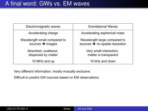
A final word: GWs vs. EM waves

12

Astrophysics with GWs vs. EM

Very different information, mostly mutually exclusive.

Difficult to predict GW sources based on EM observations.

10 kHz and down10 MHz and up

Very small interaction;

matter is transparent

Absorbed, scattered,

dispersed by matter

Wavelength large compared to

sources ! no spatial resolution

Wavelength small compared to

sources ! images

Accelerating aspherical massAccelerating charge

Gravitational WavesElectromagnetic waves


Date post:	28-Mar-2020
Category:	Documents
Upload:	others
View:	10 times
Download:	0 times

Introduction to General Relativity and Gravitational …...Introduction to General Relativity and...

Documents