Introduction to Linear Regression AnalysisInterpretation of Results

Samuel Nocito

Lecture 2

March 8th, 2018

Lecture 1 Summary

I Why and how we use econometric tools in empiricalresearch.

I Ordinary Least Square (OLS) estimation methodI simple theoretical framework;I graphical representation;I coe�cient estimation in the simple case with one regressor

(little algebra!);I practical example using NLS data on wages.

OLS: Dependent and Explanatory Variables

yi = β0 + β1Xi + εi

where:

I yi dependent variable (explained, response or predictedvariable);

I xi independent variable (explanatory, control orpredictor variable).

I εi is the error term.

OLS: De�nition of the Variables

Either dependent or independent variables can be:

I CONTINUOUS yci (or xci ) taking any real value;

I DUMMY ydi (or xdi ) taking values 1 (if yes) and 0 (if no)(e.g., variable Male of the wage example);

I LOGARITHMIC ln(yi) (or ln(xi)) simply the naturallogarithm of a continuous variable.

The interpretation of the coe�cient estimates changesaccording to the combination of these types of variables.

OLS Coe�cient Interpretation: Continuous Dep. Variable

Model A: continuous dependent variable.

yci = β0 + β1xc1i + β2ln(x2i) + β3x

d3i + εi

I β1 = a one unit change in xc1i generates a β1 unit changein yci .

I β2 = a 100% change in x2i generates a β2 change in yci .

I β3 = the movement of xd3i from 0 to 1 produces a β3 unitchange in yci .

OLS Coe�cient Interpretation: Dummy Dep. Variable

Model B: dummy dependent variable.

ydi = β0 + β1xc1i + β2ln(x2i) + β3x

d3i + εi

I β1 = a one unit change in xc1i generates a 100β1 percentagepoints change in the probability ydi occurs.

I β2 = a 100% change in x2i generates a 100β2 percentagepoints change in the probability ydi occurs.

I β3 = the movement of xd3i from 0 to 1 produces a 100β3percentage points change in the probability ydi occurs.

OLS Coe�cient Interpretation: log Dep. Variable

Model C: logarithm dependent variable.

ln(yi) = β0 + β1xc1i + β2ln(x2i) + β3x

d3i + εi

I β1 = a one unit change in xc1i generates a 100β1 percentchange in yi.

I β2 = a 100% change in x2i generates a 100β2 percentchange in yi.

I β3 = the movement of xd3i from 0 to 1 produces a 100β3percent change in yi.

OLS Coe�cient Interpretation: Wage Example

Wagei = β0 + β1Malei + εi

This is a model of type A ⇒ continuous dep. variable and β1refers to a DUMMY explanatory variable (Male).

Table: OLS results wage equation (Verbeek, tab. 2.1)

Dependent variable: wage

Variable Estimate Standard Error

Constant 5.1469 0.0812

Male 1.1661 0.1122

R2 = 0.0317 F=107.93

Wagei = 5.15 + 1.17Malei

I β1 = the movement of Male from 0 to 1 produces a β1(1.17) unit change in Wagei.

Types of Data

There are four di�erent types of data:

I Cross-sectional: sample of observations taken at a givenpoint in time.

I Time series: observations on a variable or severalvariables over time.

I Pooled cross-sectional: di�erent random samples areasked the same questions over time.

I Panel (or longitudinal): consists of a time series onsame individuals (i.e., ask to Sarah the same question intwo di�erent years).

Coe�cient Interpretation in the Literature: Example 1

I Does foreign language pro�ciency foster migration

of young individual within the European Union?

(Aparicio Fenoll and Kuehn, 2016)

Model equation (of type A):

Ma,o,d,t = β0 + β1La,o,d,t + ...+ εa,o,d,t

I M: number of immigrants of age a from country o to din year t.

I L: exposure to compulsory language courses in theo�cial language of country d.

I Other controls (i.e., dummies and predetermined controlsas unemployment rate).

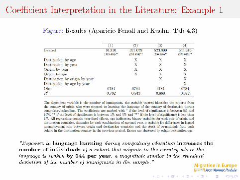
Coe�cient Interpretation in the Literature: Example 1

Figure: Results (Aparicio Fenoll and Kuehn, Tab 4.3)

"Exposure to language learning during compulsory education increases the

number of individuals of a cohort that migrate to the country where the

language is spoken by 544 per year, a magnitude similar to the standard

deviation of the number of immigrants in the sample."

OLS Endogeneity Issues

Endogeneity occurs whenever the explanatory variable(regressor) is correlated with the error term.

Endogeneity conditions:

I Measurement error: error made in measuring the dependentor the explanatory variable.

Example: wages is an information that people not alwayswant to provide. Di�cult to measure the sampleinformation ⇒ data itself correlated with the error.

OLS Endogeneity Issues

Endogeneity conditions:

I Reverse causality: x⇒ y (what we look for), y ⇒ x(reverse causality), or y ⇔ x (simultaneity).

Example (police and crime): increased police force mightcause a reduction in crime, however an increase/decrease incrime might cause an increase/decrease in policemannumber.

I Omitted variable: some unobservable variables a�ectingboth y and x.

Example: ability a�ects both education and wages ⇒return on education is a di�cult question.

OLS results often a�ected by endogeneity.Infer causality with OLS is hard and rare.

Correlation vs Causality

I Correlation is a statistical measure describing the size andthe direction of a relationship between two or morevariables.

I Causality indicates that one event is the result of theoccurrence of the other event.1

Example 1: Smoking might be correlated with alcoholism butit is not a cause of it.Example 2: Immigration might be correlated to the total levelof crime in a speci�c region or province, however it is not adirect cause of it (see next example).

I Causality is compromised by endogeneity

⇒ other driven factors a�ecting the choice.

1Australian Bureau of Statistics.

Instrumental Variable (IV): basic concept

Crimep = β0 + β1Immigrantsp + εp

Suppose we want to measure the impact of immigrants on crimeat province (p) level.

I The choice of migrating in a particular province isendogenous. ⇒ we can see only correlation.

I We can use an Instrumental Variable to investigatecausality.

The Instrument must be:

I Assumption 1: (strongly) correlated with the endogenousvariable.

I Assumption 2: independent of y (exogenous).

I Assumption 3: built to a�ect all the treated in the sameway.

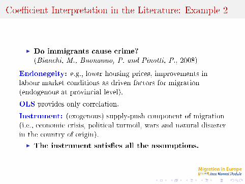
Coe�cient Interpretation in the Literature: Example 2

I Do immigrants cause crime?

(Bianchi, M., Buonanno, P. and Pinotti, P., 2008)

Endonegeity: e.g., lower housing prices, improvements inlabour market conditions as driven factors for migration(endogenous at provincial level).

OLS provides only correlation.

Instrument: (exogenous) supply-push component of migration(i.e., economic crisis, political turmoil, wars and natural disasterin the country of origin).

I The instrument satis�es all the assumptions.

Coe�cient Interpretation in the Literature: Example 2(OLS)

Figure: OLS Results (Bianchi et al., Tab 3)

Coe�cient Interpretation in the Literature: Example 2(IV)

Figure: OLS vs IV Results (Bianchi et al., Tab 4)

I Total crime is not related to the size of immigrants (IV).

I NO statistically signi�cant result in the IV.

I POSITIVE and statistically signi�cant correlation.NO causality e�ect.

Summary

I OLS as a tool to answer economic questions.

I OLS implies correlation but not always causality.

I IV can infer causality under certain assumptions.

I The variable types (log, dummy, etc.) determine thecoe�cient interpretation.

I Standard errors show the magnitude of the estimation error(the smaller the better!).

I Statistic signi�cance (stars!) to see if the estimatedcoe�cient is statistically signi�cantly di�erent from 0.

I R2 is the fraction of the sample variation in y that isexplained by x.

References

I APARICIO FENOLL, Ainhoa; KUEHN, Zoë. Does foreignlanguage pro�ciency foster migration of young individualswithin the European Union. The economics of language

policy, 2016, 331-355.

I BIANCHI, Milo; BUONANNO, Paolo; PINOTTI, Paolo.Do immigrants cause crime?. Journal of the European

Economic Association, 2012, 10.6: 1318-1347.