102
Introduction to Signals and Systems Lectures #3 - State-space Representation of Systems Guillaume Drion Academic year 2017-2018 1

Introduction to Signals and Systems Lectures #3 - State-space Representation of Systems
Guillaume Drion Academic year 2017-2018
1
Outline
Modeling in state-space - time invariance - linearity
Block diagram and state-space representation (discrete and continuous)
Solutions of state-space equations: transition matrix and matrix exponential
Response of N-dimensional systems
2

Systems modeling
Modeling and analysis of systems: open loop. “Observing and analyzing the environment”
Can be used to understand/analyze the behavior of a dynamical system. A “good” model can predict the future evolution of a system.
How can we use systems modeling to predict the future? What is a “good model” or a “good system” to model?
SYSTEMInput Output
3

In “state-space”, dynamical systems are modeled using difference equations (discrete domain) or differential equations (continuous domain).
4
, are variables of the systems (the model describes their evolution). A system can have many variables (dimension).x[n]
is a parameter of the system. A system can have many parameters.a
x =dx
dt
(where )x[n+ 1] = ax[n]
! x[n] = a
n
x = ax
! x(t) = e
at
Discrete domain Continuous domain
x(t)

In “state-space”, dynamical systems are modeled using difference equations (discrete domain) or differential equations (continuous domain).
5
, are variables of the systems (the model describes their evolution). A system can have many variables (dimension).x[n]
is a parameter of the system. A system can have many parameters.a
x =dx
dt
(where )x[n+ 1] = ax[n]
! x[n] = a
n
x = ax
! x(t) = e
at
Discrete domain Continuous domain
x(t)
What defines a parameter?

Time-variance vs time-invariance
Example: think about the evolution of a stock market.
Can we accurately predict the evolution of a stock market using a model?
where the evolution depends on the market growth rate, i.e the market growth rate is a parameter of the system.
6
Time-variance vs time-invariance
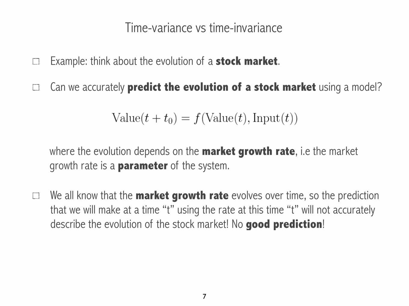
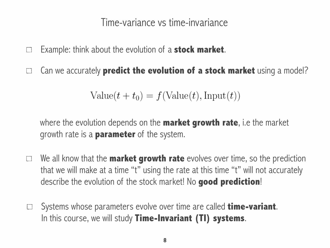
Example: think about the evolution of a stock market.
Can we accurately predict the evolution of a stock market using a model?
We all know that the market growth rate evolves over time, so the prediction that we will make at a time “t” using the rate at this time “t” will not accurately describe the evolution of the stock market! No good prediction!
where the evolution depends on the market growth rate, i.e the market growth rate is a parameter of the system.
7
Time-variance vs time-invariance
Example: think about the evolution of a stock market.
Can we accurately predict the evolution of a stock market using a model?
We all know that the market growth rate evolves over time, so the prediction that we will make at a time “t” using the rate at this time “t” will not accurately describe the evolution of the stock market! No good prediction!
Systems whose parameters evolve over time are called time-variant. In this course, we will study Time-Invariant (TI) systems.
where the evolution depends on the market growth rate, i.e the market growth rate is a parameter of the system.
8

Time-Invariant (TI) systems
In a time-invariant system, the input/output relationship does not depend on time:
i.e. a system whose parameters do not vary over time!
if then
Examples: is time-invariant. is time-variant.
9
In this course, we focus in time-invariant systems.

State-space representation in continuous-time: general form
General form of a state-space representation in continuous-time:
is the input is the output, are the states (i.e. energy storage/memory).
!! State-space representations are not unique !! But all representations describe the same system, i.e. with the same (and unique) inputs, outputs and transfer function.
10
u(t)y(t)x(t)
State-space representation in continuous-time: identifying states
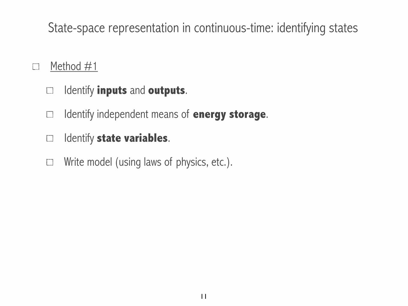
Method #1
Identify inputs and outputs.
Identify independent means of energy storage.
Identify state variables.
Write model (using laws of physics, etc.).
Method #2
Write model (using laws of physics, etc.).
Identify inputs and outputs.
Identify state variables.
11

State-space representation in continuous-time: identifying states
Method #1
Identify inputs and outputs.
Identify independent means of energy storage.
Identify state variables.
Write model (using laws of physics, etc.).
Method #2
Identify inputs and outputs.
Write model (using laws of physics, etc.).
Identify state variables.
12

Modeling TI systems in state-space: driven pendulum
u
θ
m
l
mg
13

Driven pendulum: modelingu
θ
m
l
mg with moment of inertia.
which gives .
What do I do with a ? vs
14

Driven pendulum: statesu
θ
m
l
mg with moment of inertia.
which gives .
What do I do with a ? vs
States: . If I want to write the system in the form , the second state should be (the energy is stored in the position and speed).
15
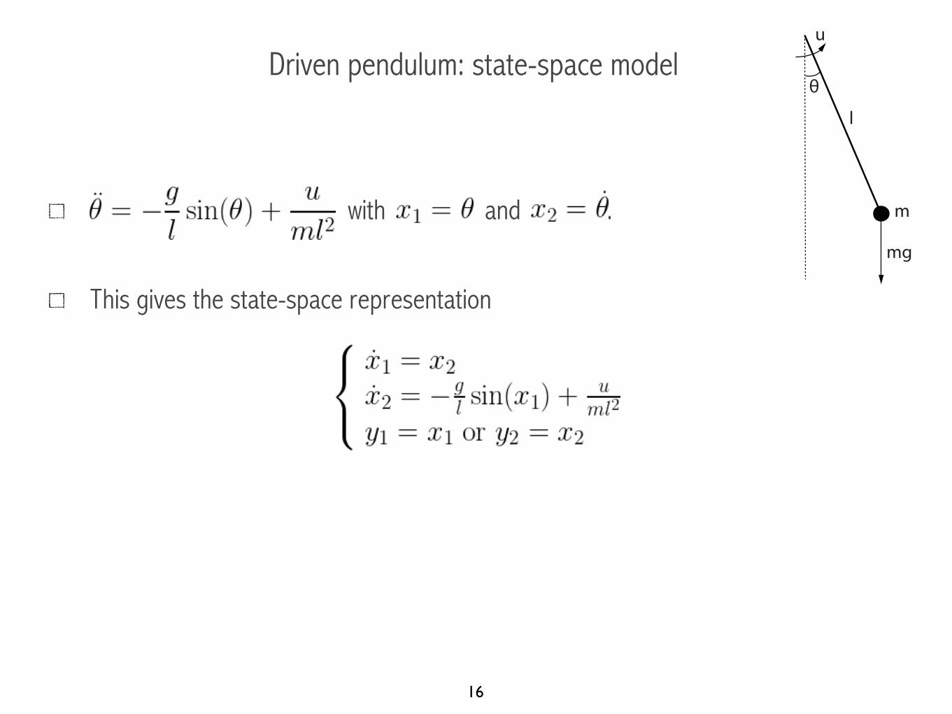
Driven pendulum: state-space modelu
θ
m
l
mg
with and .
This gives the state-space representation
16

Driven pendulum: model analysisu
θ
m
l
mg
with and .
This gives the state-space representation
(i) Is the system linear? No!
17
Nonlinear vs linear models
18
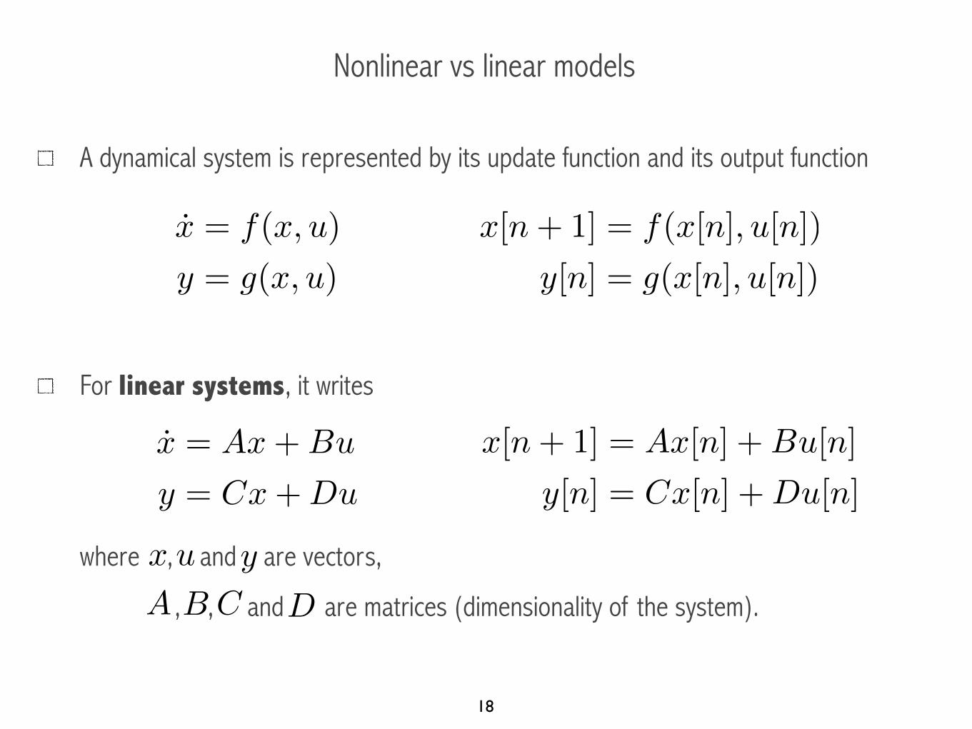
A dynamical system is represented by its update function and its output function
For linear systems, it writeswhere , and are vectors,
, , and are matrices (dimensionality of the system).
x = f(x, u)
y = g(x, u)
x = Ax+Bu
y = Cx+Du
BA
x u y
DC
x[n+ 1] = Ax[n] +Bu[n]
y[n] = Cx[n] +Du[n]
x[n+ 1] = f(x[n], u[n])
y[n] = g(x[n], u[n])

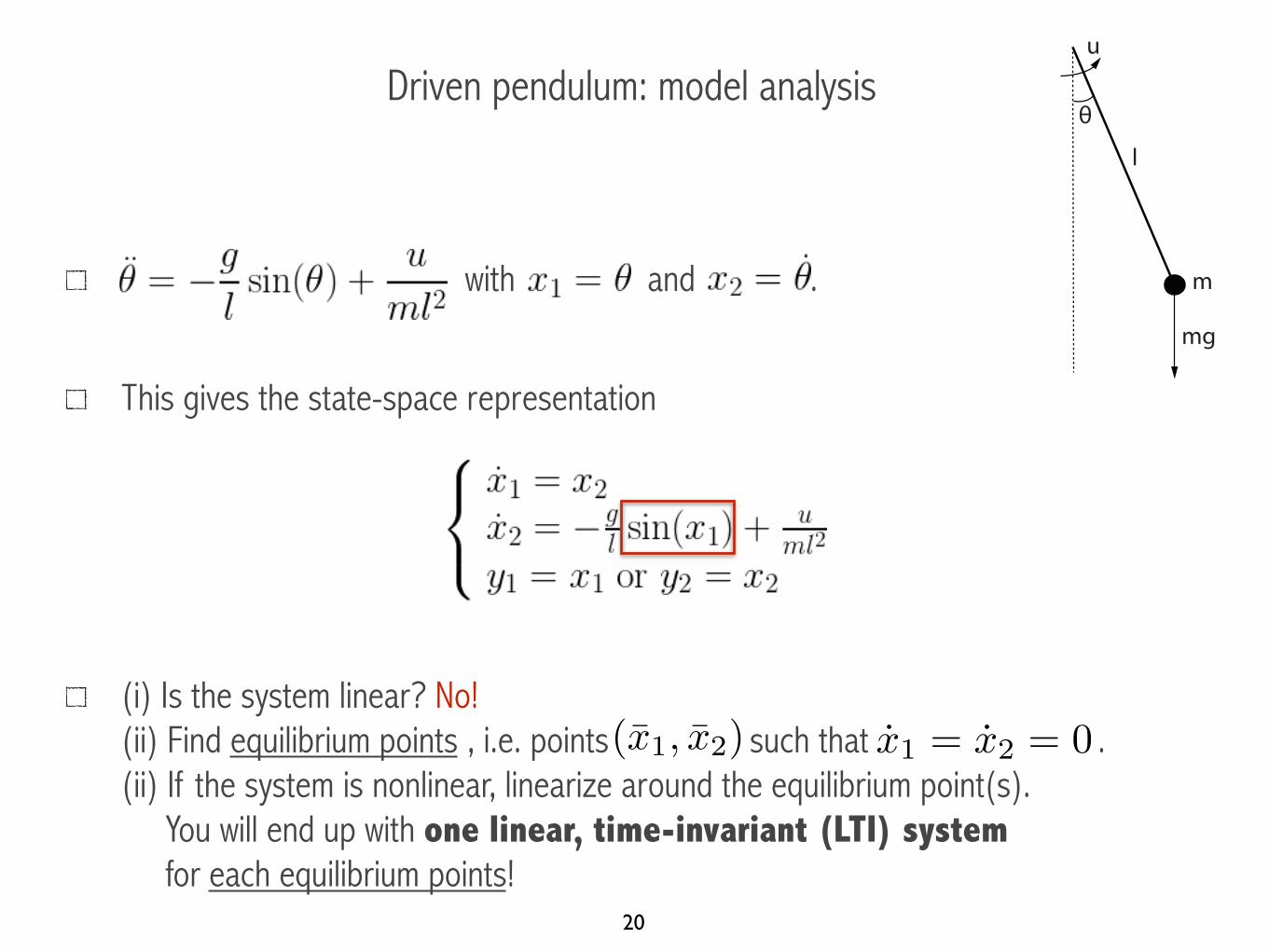
Driven pendulum: model analysisu
θ
m
l
mg
with and .
This gives the state-space representation
(i) Is the system linear? No! (ii) Find equilibrium points , i.e. points such that .
19
(x1, x2) x1 = x2 = 0
Driven pendulum: model analysisu
θ
m
l
mg
with and .
This gives the state-space representation
(i) Is the system linear? No! (ii) Find equilibrium points , i.e. points such that . (ii) If the system is nonlinear, linearize around the equilibrium point(s). You will end up with one linear, time-invariant (LTI) system for each equilibrium points!
20
(x1, x2) x1 = x2 = 0

Driven pendulum: linearizationu
θ
m
l
mgIdea behind linearizing a system around a specific point:
x
f(x)
+ See tutorials.
21
x = f(x, u)
y = g(x, u)
x = Ax+Bu
y = Cx+Du

Modeling LTI system: a RC circuit
R
CV
i
vC(t)vR(t)
22
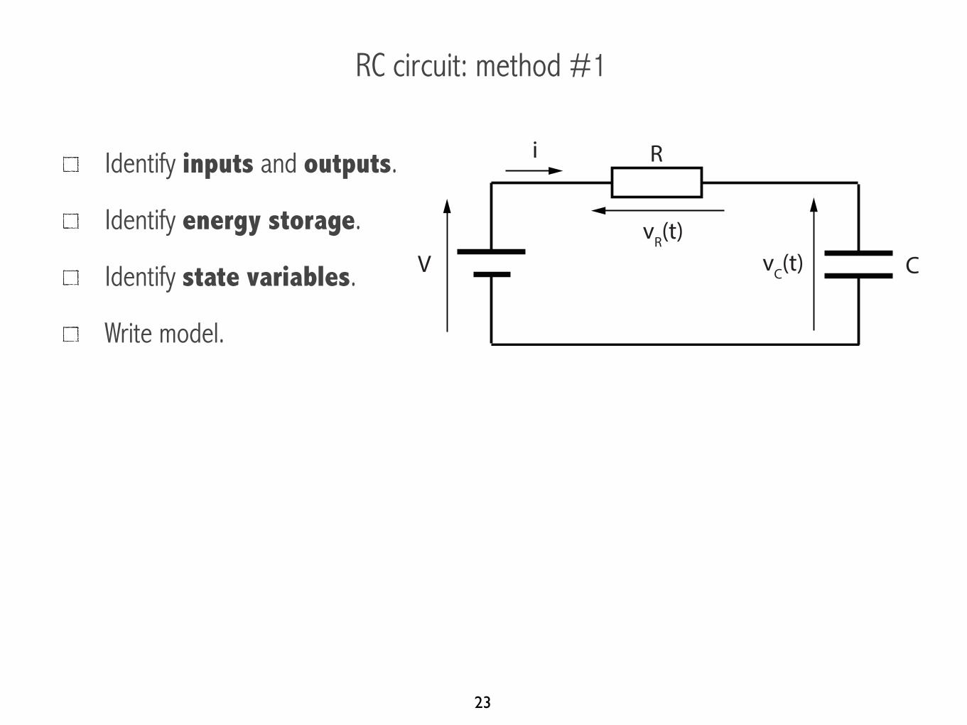
RC circuit: method #1
Identify inputs and outputs.
Identify energy storage.
Identify state variables.
Write model.
R
CV
i
vC(t)vR(t)
23

RC circuit: method #1 - inputs and outputs
Identify inputs and outputs.
Identify energy storage.
Identify state variables.
Write model.
Inputs: active sources voltage source:
Outputs: or
R
CV
i
vC(t)vR(t)
24
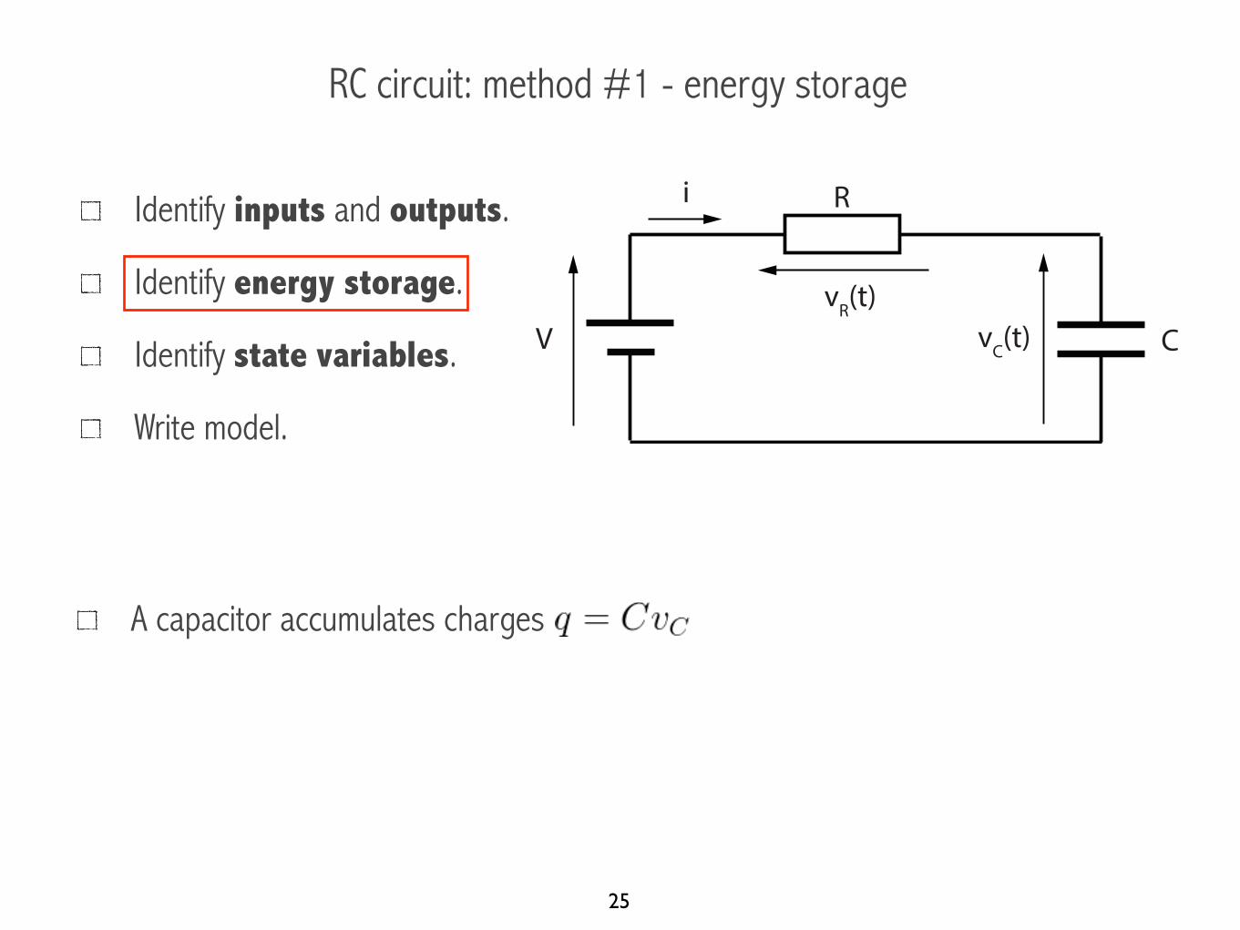
RC circuit: method #1 - energy storage
Identify inputs and outputs.
Identify energy storage.
Identify state variables.
Write model.
A capacitor accumulates charges
R
CV
i
vC(t)vR(t)
25

RC circuit: method #1 - state variables
Identify inputs and outputs.
Identify energy storage.
Identify state variables.
Write model.
A capacitor accumulates charges
State variable:
R
CV
i
vC(t)vR(t)
26

RC circuit: method #1 - model
Identify inputs and outputs.
Identify energy storage.
Identify state variables.
Write model.
R
CV
i
vC(t)vR(t)
Input: . Output: or . State:
Kirchhoff:
Which gives
27

RC circuit: method #2
Identify inputs and outputs.
Write model
Identify state variables.
R
CV
i
vC(t)vR(t)
28

RC circuit: method #2 - model
Identify inputs and outputs.
Write model
Identify state variables.
Input: . Output: or .
Kirchhoff:
State variable:
R
CV
i
vC(t)vR(t)
29

RC circuit: method #2 - state variable
Identify inputs and outputs.
Write model
Identify state variables.
Input: . Output: or .
Kirchhoff:
State variable:
R
CV
i
vC(t)vR(t)
30

RC circuit: method #2 - state-space model
Identify inputs and outputs.
Write model
Identify state variables.
Input: . Output: or . State:
Kirchhoff:
Which gives
R
CV
i
vC(t)vR(t)
31
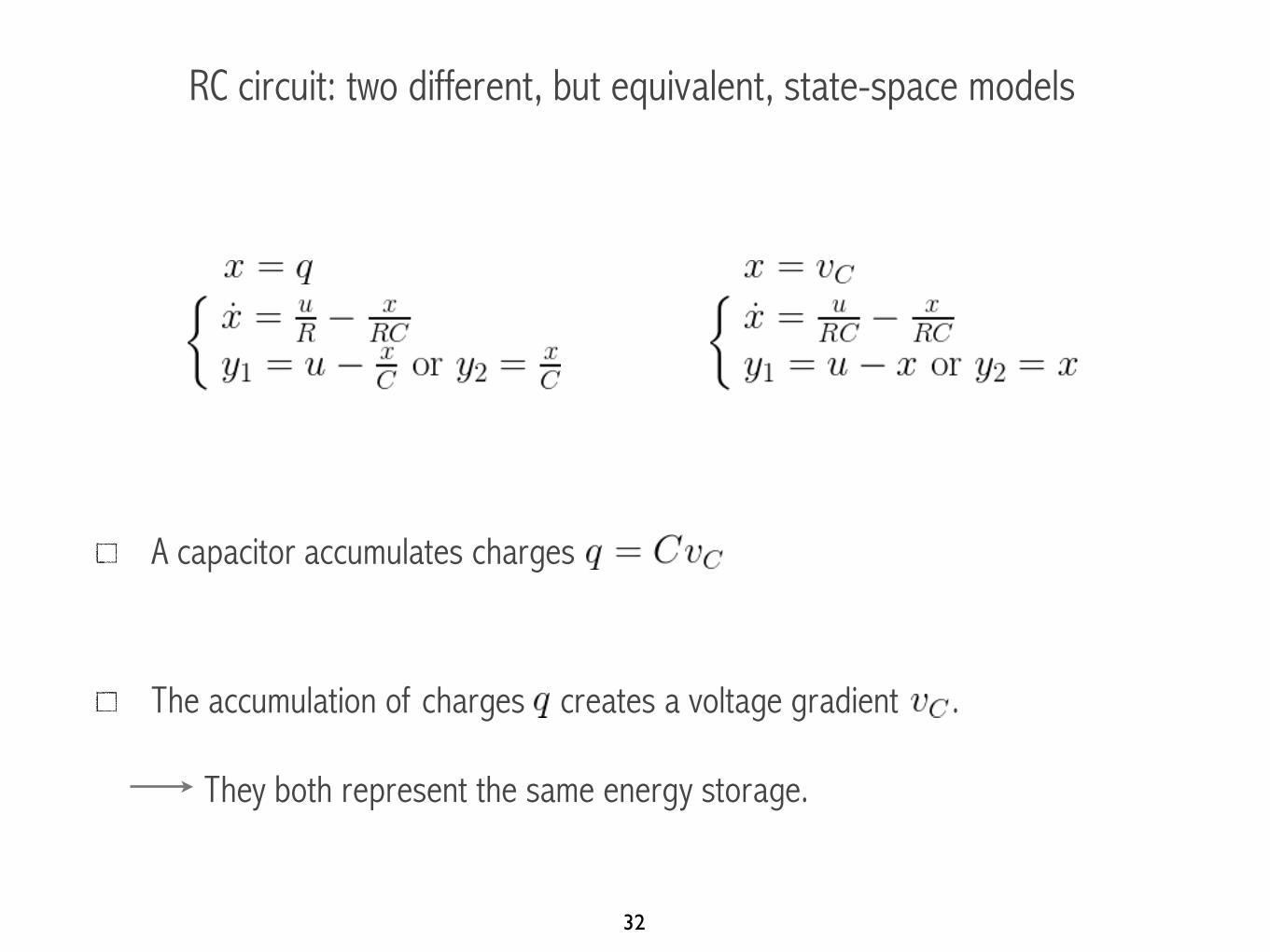
RC circuit: two different, but equivalent, state-space models
A capacitor accumulates charges
The accumulation of charges creates a voltage gradient . They both represent the same energy storage.
32

RLC circuit: inputs, outputs, states, equations
R
LV
i
vL(t)vR(t)
C
vC(t)
Identify inputs and outputs.
Identify energy storage.
Identify state variables.
Write model.
Input: . Output: or or .
Energy storage/variable. Capacitor: . Inductor: .
Kirchhoff:
33

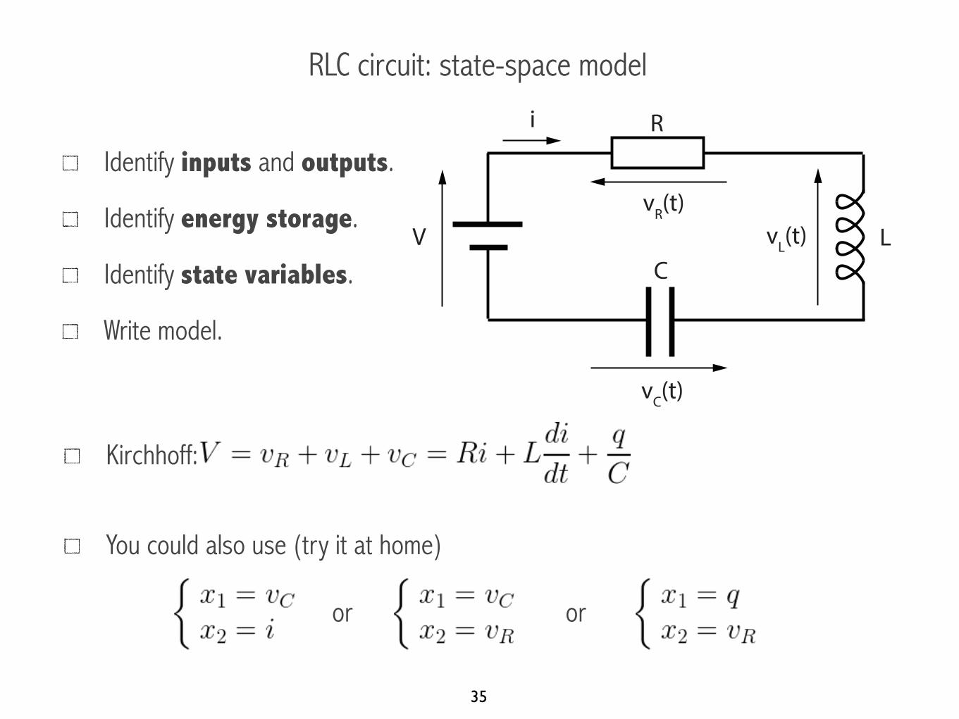
RLC circuit: state-space model
R
LV
i
vL(t)vR(t)
C
vC(t)
Identify inputs and outputs.
Identify energy storage.
Identify state variables.
Write model.
Kirchhoff: with and .
State-space model:
34
RLC circuit: state-space model
R
LV
i
vL(t)vR(t)
C
vC(t)
Identify inputs and outputs.
Identify energy storage.
Identify state variables.
Write model.
Kirchhoff:
You could also use (try it at home) or or
35

Outline
Modeling in state-space - time invariance - linearity
Block diagram and state-space representation (discrete and continuous)
Solutions of state-space equations: transition matrix and matrix exponential
Response of N-dimensional systems
36

State-space representation of LTI systems
37
A LTI system can be represented as followswhere is the state vector whose dimension gives the dimension of the system.
In a single-input/single-output (SISO) system, we have (ex: 4 states)
State-space representation of LTI systems
38
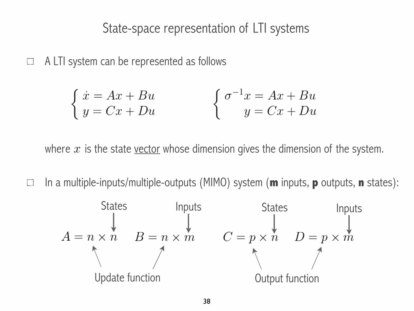
A LTI system can be represented as followswhere is the state vector whose dimension gives the dimension of the system.
In a multiple-inputs/multiple-outputs (MIMO) system (m inputs, p outputs, n states):
Update function Output function
States Inputs States Inputs
State-space representation of LTI systems
39
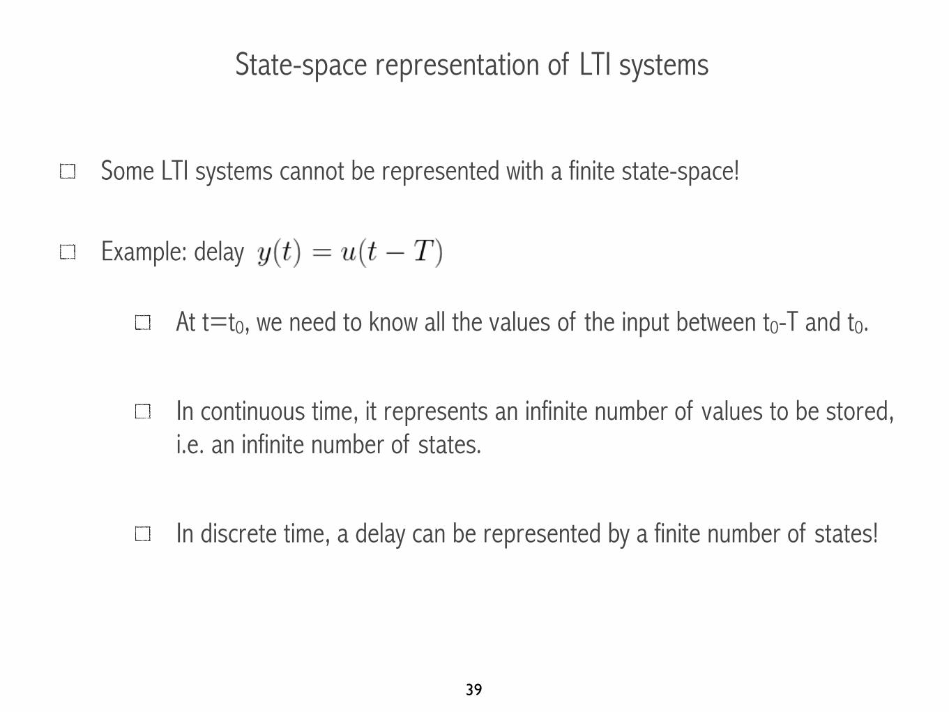
Some LTI systems cannot be represented with a finite state-space!
Example: delay
At t=t0, we need to know all the values of the input between t0-T and t0.
In continuous time, it represents an infinite number of values to be stored, i.e. an infinite number of states.
In discrete time, a delay can be represented by a finite number of states!

State-space representation of LTI systems
40
What kind of LTI systems admit a state-space representation?
Continuous time:
Discrete time:
yes if
yes if
State-space representation of LTI systems in continuous time
41
We will derive a general structure for the state-space representation of LTI systems in continuous time.
Let’s start with a first order system (i.e. one state):
This system can be done with one integrator (not a differentiator!!!), multipliers, and one adder (or summer).
We will start by building a block diagram of the system using integrators, multipliers and adders.
Block diagram of a first order system in continuous time
42
Block diagram of the first order system

Block diagram of a first order system in continuous time
43
Block diagram of the first order system

Block diagram of a first order system in continuous time
44
Block diagram of the first order system

Block diagram of a first order system in continuous time
45
Block diagram of the first order system
y goes back in u for the next “update”. effect of the past value of y!

Block diagram of a first order system in continuous time
46
Block diagram of the first order system
Input-output approach using the block diagram: If , we have

Block diagram of a first order system in continuous time
47
Block diagram of the first order system
Let’s define a state in which we store the history of the system (here, ):
Block diagram of a first order system in continuous time
48
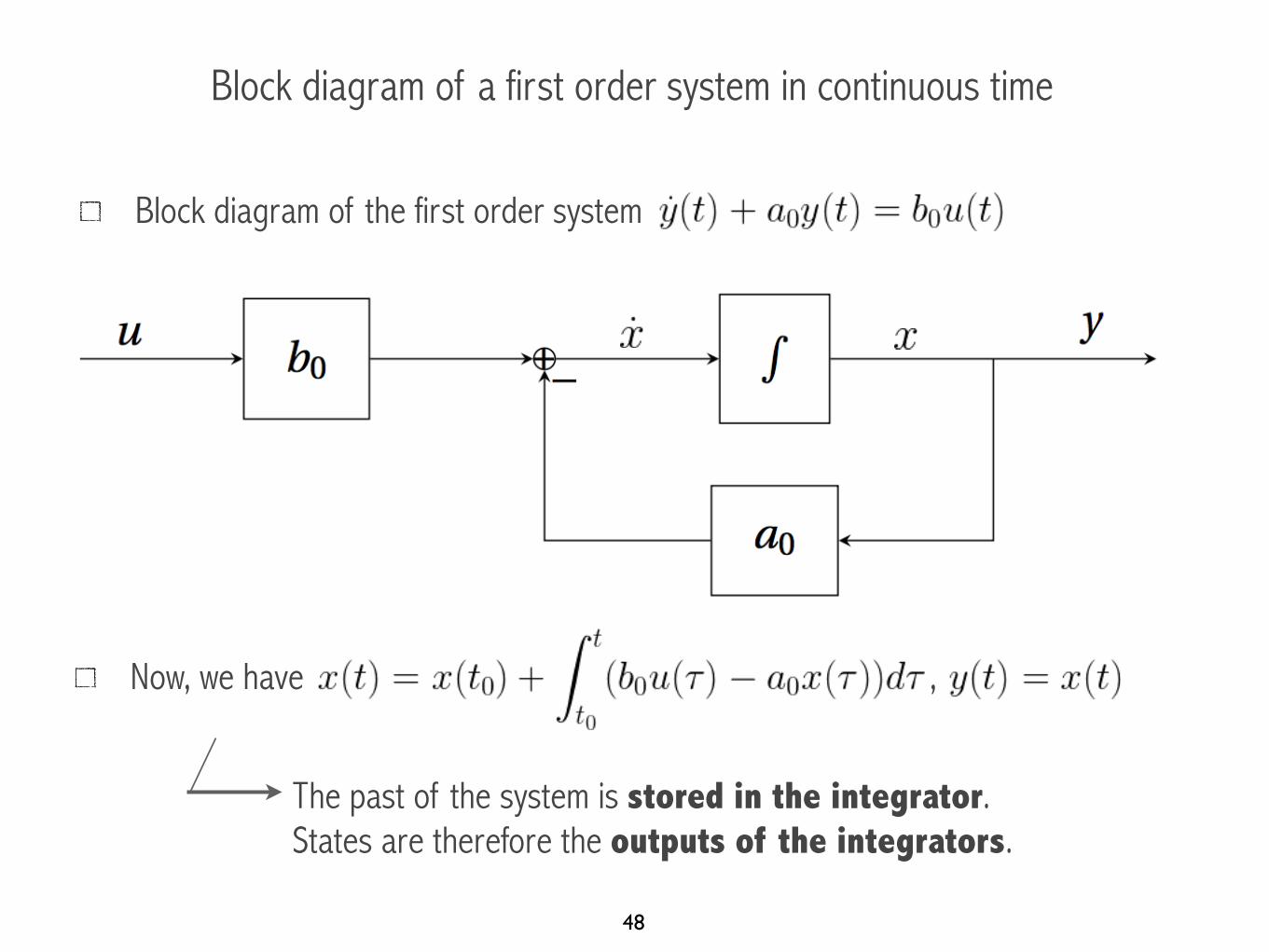
Block diagram of the first order system
Now, we have ,
The past of the system is stored in the integrator. States are therefore the outputs of the integrators.

The past of the system (or energy) is stored in the integrators
49
t
y
t0 t0+t1
At t=t0+t1, the integral contains the history of the past values.

State-space representation/block diagram in continuous time
50
Block diagram: representation of the system using integrators.
State-space: representation of the system using states, which are the outputs of the integrators!
Example: RLC circuitthe current in the inductor and the voltage across the capacitor are outputs of integrators!

A N-dimensional system in continuous time
51
Let’s first consider the case
Which can be written(incorrect in the book)

Block diagram of a N-dimensional system in continuous time
52

Block diagram of a N-dimensional system in continuous time
53

Block diagram of a N-dimensional system in continuous time
54

Block diagram of a N-dimensional system in continuous time
55

Block diagram of a N-dimensional system in continuous time
56
States are outputs of integrators:

State-space representation of a N-dimensional system in continuous time
57
States are outputs of integrators:
8>>>>>>>>><
>>>>>>>>>:
x1 = x2
x2 = x3
x3 = x4...xn�1 = xn
xn = �a0x1 � a1x2 � . . .� aN�1xn + b0u
y = x1

A general N-dimensional system in continuous time
58
Let’s now consider the general case
We have to consider an intermediate signal where
Justification:
and
P (D)y = Q(D)u ( P (D)⌫ = u and y = Q(D)⌫

Block diagram of a general N-dimensional system in continuous time
59
and

Block diagram of a general N-dimensional system in continuous time
60
and
Block diagram of a general N-dimensional system in continuous time
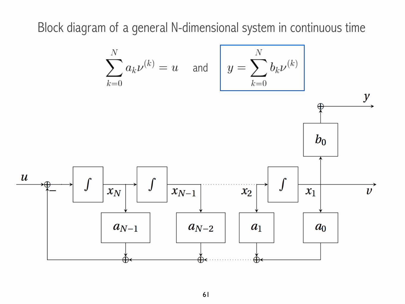
61
and
Block diagram of a general N-dimensional system in continuous time
62
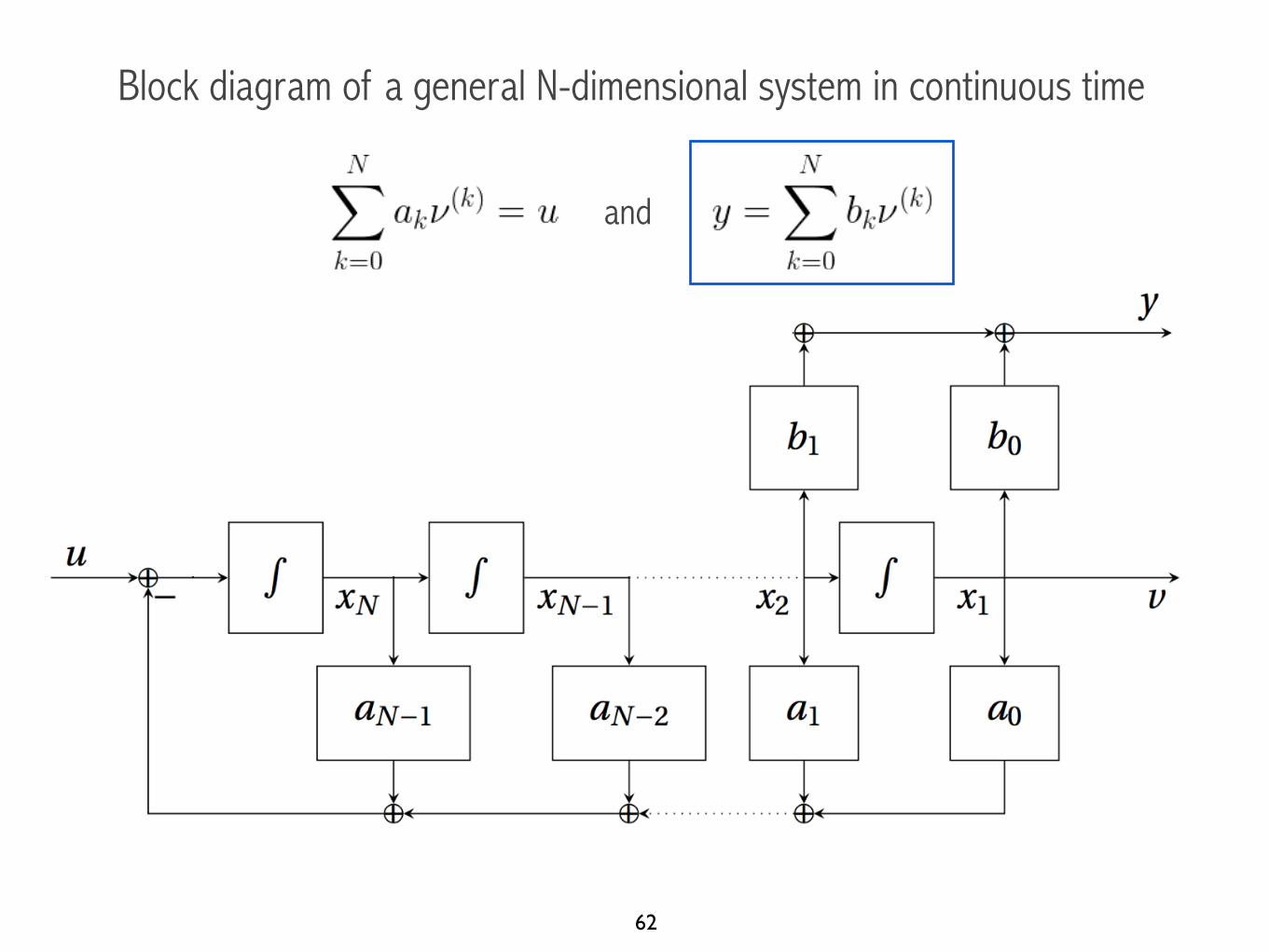
and

Block diagram of a general N-dimensional system in continuous time
63
and
State-space of a general N-dimensional system in continuous time
64
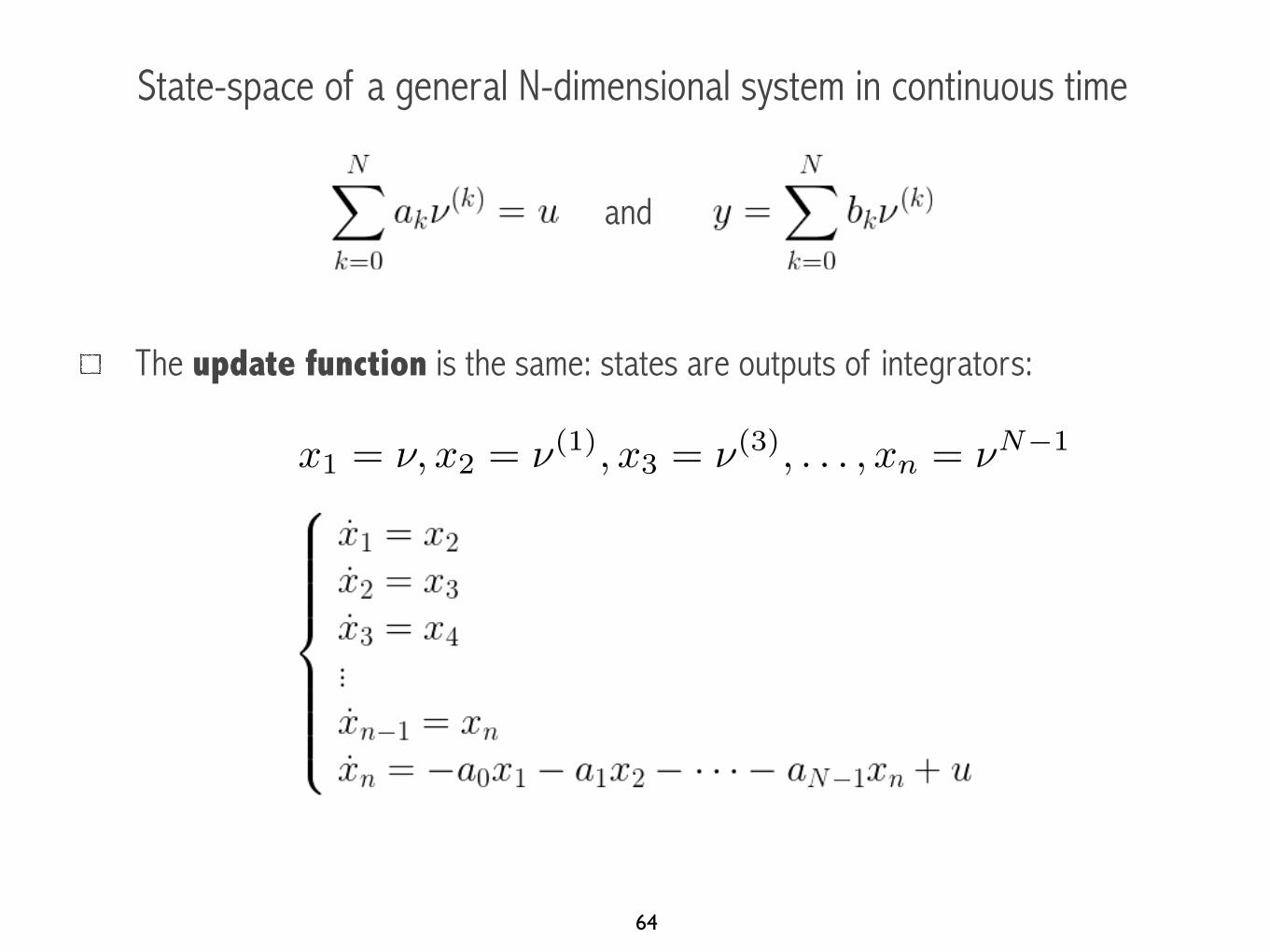
and
The update function is the same: states are outputs of integrators:
x1 = ⌫, x2 = ⌫
(1), x3 = ⌫
(3), . . . , xn = ⌫
N�1

State-space of a general N-dimensional system in continuous time
65
and
The output function is more complex:
x1 = ⌫, x2 = ⌫
(1), x3 = ⌫
(3), . . . , xn = ⌫
N�1
State-space of a general N-dimensional system in continuous time
66
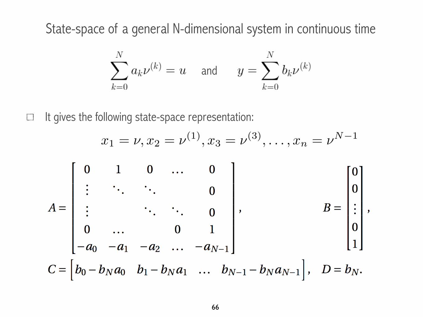
and
It gives the following state-space representation:
x1 = ⌫, x2 = ⌫
(1), x3 = ⌫
(3), . . . , xn = ⌫
N�1

State-space representation of LTI systems in discrete time
67
We will derive a general structure for the state-space representation of LTI systems in discrete time.
Let’s start with a first order system (i.e. one state):
This system can be done with one delay, multipliers, and one adder (or summer).
We will start by building a block diagram of the system using delays, multipliers and adders.

Block diagram of a first order system in discrete time
68
Block diagram of the first order system

Block diagram of a first order system in discrete time
69
Block diagram of the first order system
Block diagram of a first order system in discrete time
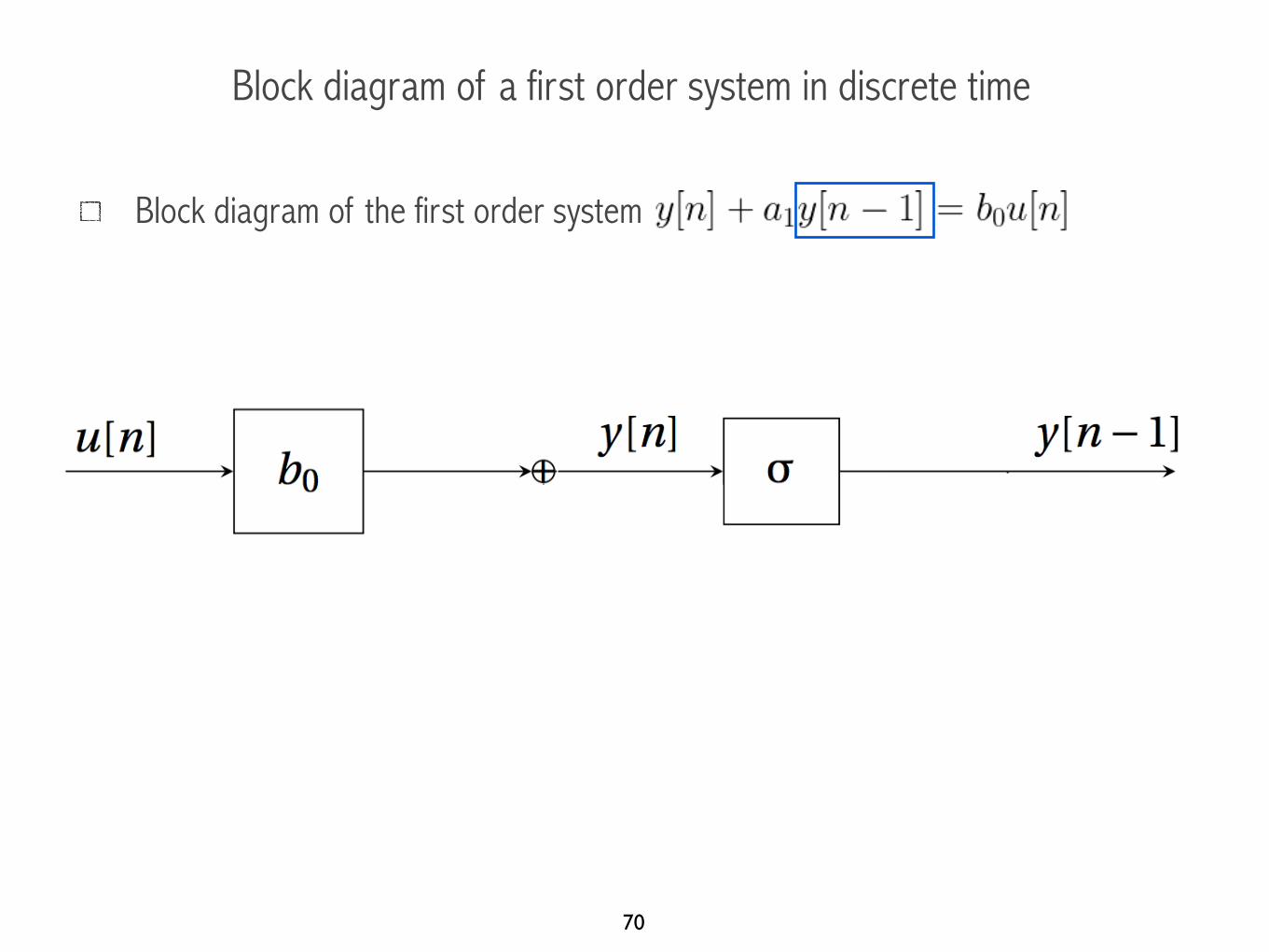
70
Block diagram of the first order system
Block diagram of a first order system in discrete time
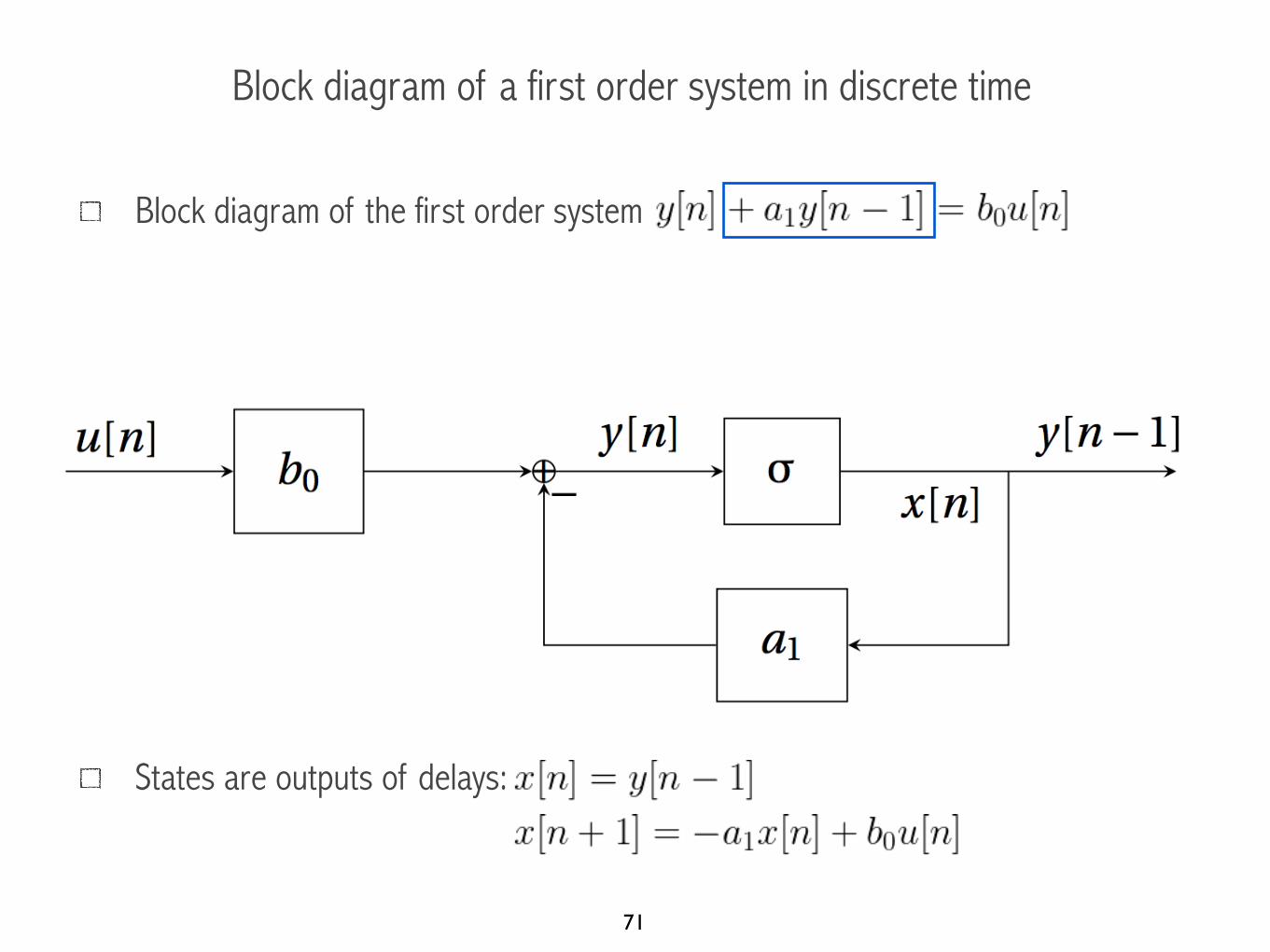
71
Block diagram of the first order system
States are outputs of delays:
A general N-dimensional system in discrete time
72
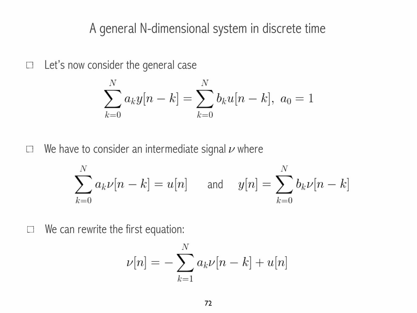
Let’s now consider the general case
We have to consider an intermediate signal where
We can rewrite the first equation:
and
State-space of a general N-dimensional system in discrete time
73
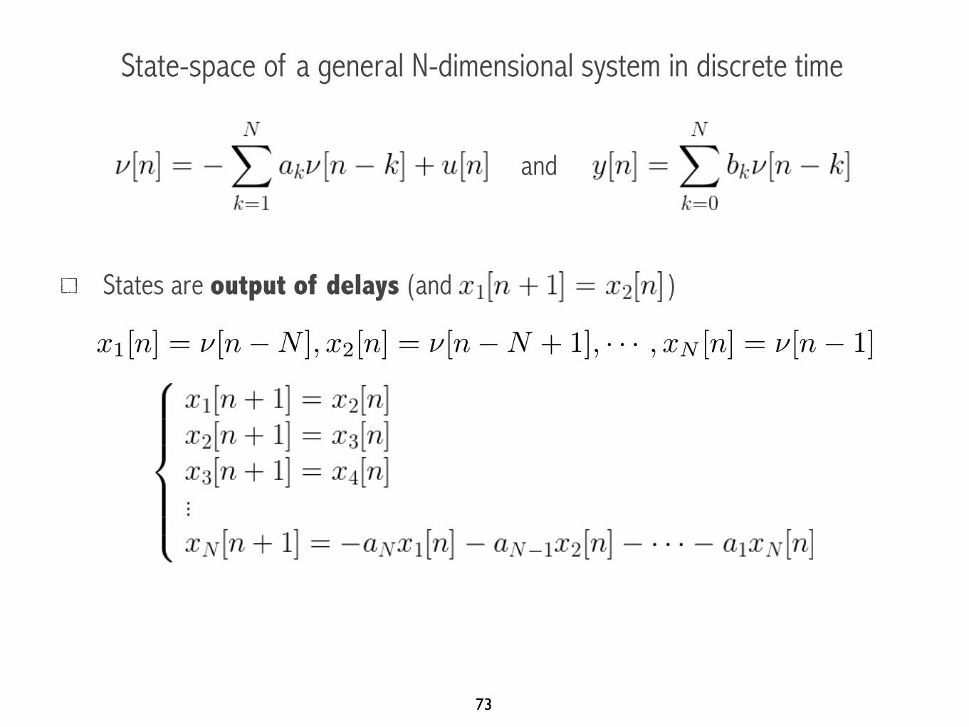
States are output of delays (and )
and
x1[n] = ⌫[n�N ], x2[n] = ⌫[n�N + 1], · · · , xN [n] = ⌫[n� 1]
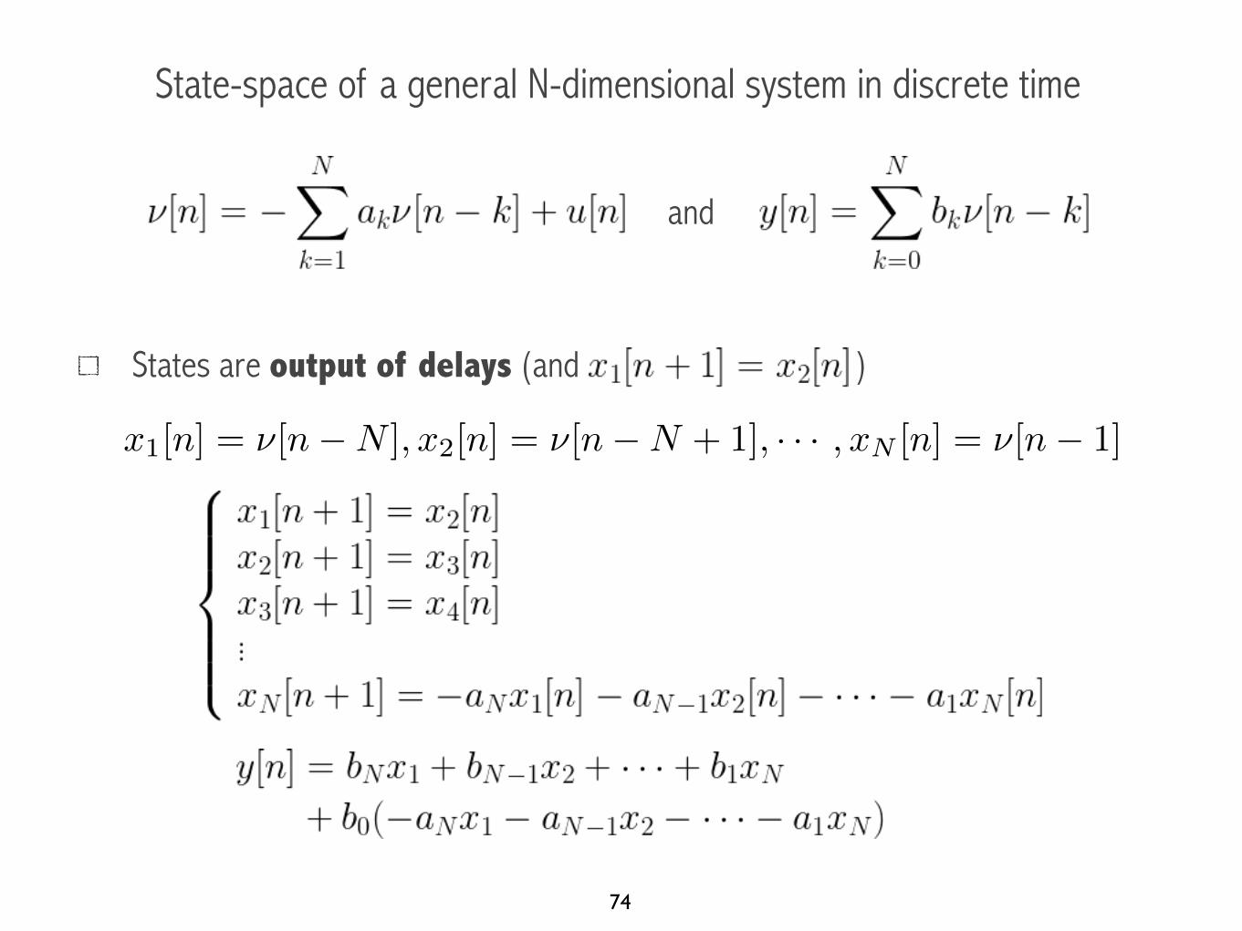
State-space of a general N-dimensional system in discrete time
74
States are output of delays (and )
and
x1[n] = ⌫[n�N ], x2[n] = ⌫[n�N + 1], · · · , xN [n] = ⌫[n� 1]
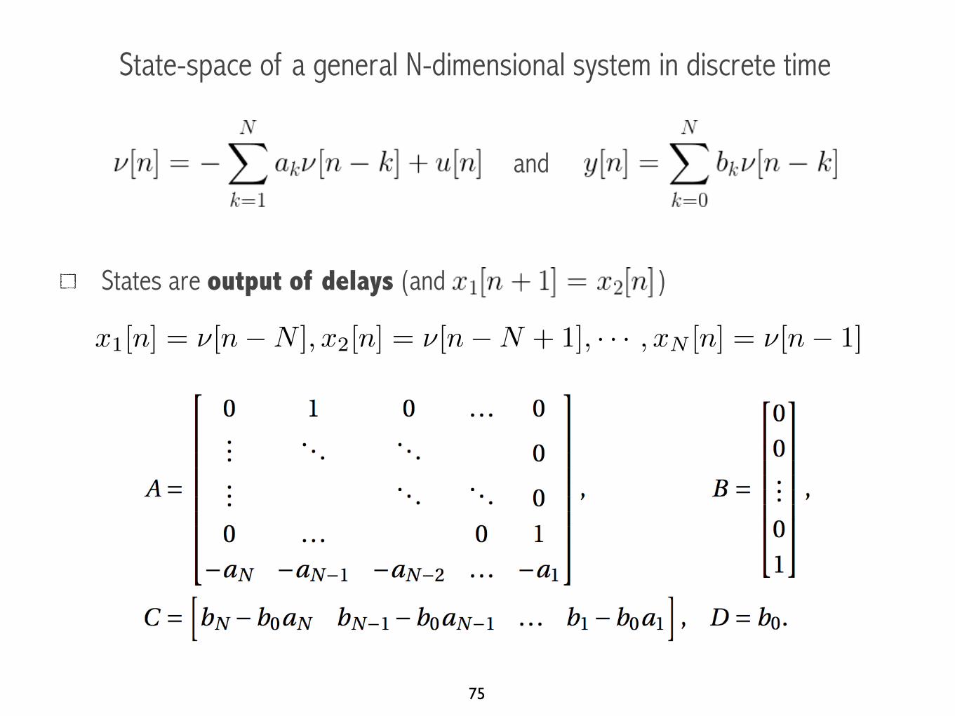
State-space of a general N-dimensional system in discrete time
75
States are output of delays (and )
and
x1[n] = ⌫[n�N ], x2[n] = ⌫[n�N + 1], · · · , xN [n] = ⌫[n� 1]
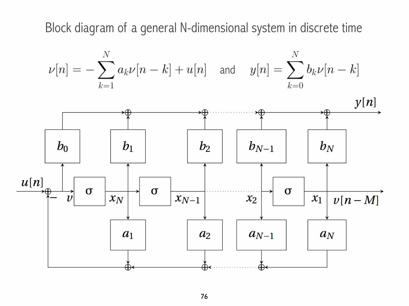
Block diagram of a general N-dimensional system in discrete time
76
and

Solutions of state-space equations: discrete case
A. Update function:
77
Outline
Modeling in state-space - time invariance - linearity
Block diagram and state-space representation (discrete and continuous)
Solutions of state-space equations: transition matrix and matrix exponential
Response of N-dimensional systems
78
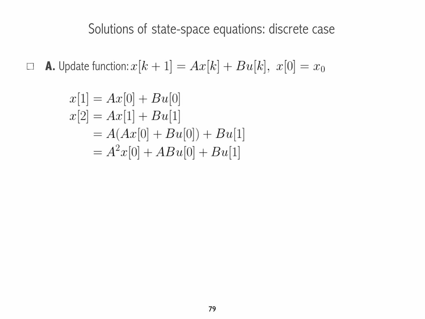
Solutions of state-space equations: discrete case
A. Update function:
79

Solutions of state-space equations: discrete case
A. Update function:
80

Solutions of state-space equations: discrete case
A. Update function:
81
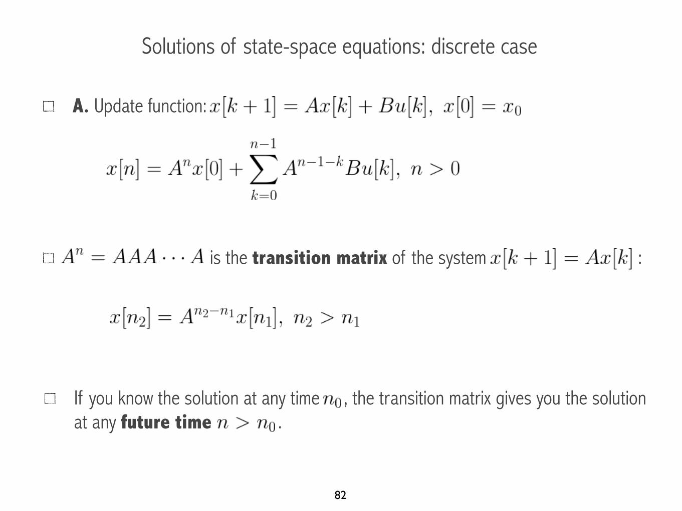
Solutions of state-space equations: discrete case
A. Update function:
is the transition matrix of the system :
If you know the solution at any time , the transition matrix gives you the solution at any future time .
82

Using we have
Solutions of state-space equations: discrete case
B. Output function:
83

Using we have
Solutions of state-space equations: discrete case
B. Output function:
zero inputzero state
84

Solutions of state-space equations: continuous case
A. Update function: .
Let’s start with the autonomous system (zero-input).
If (scalar, i.e. one dimensional case), we have , which gives the solution (zero-input response):
We want to extend this solution to the general, N-dimensional case!
85
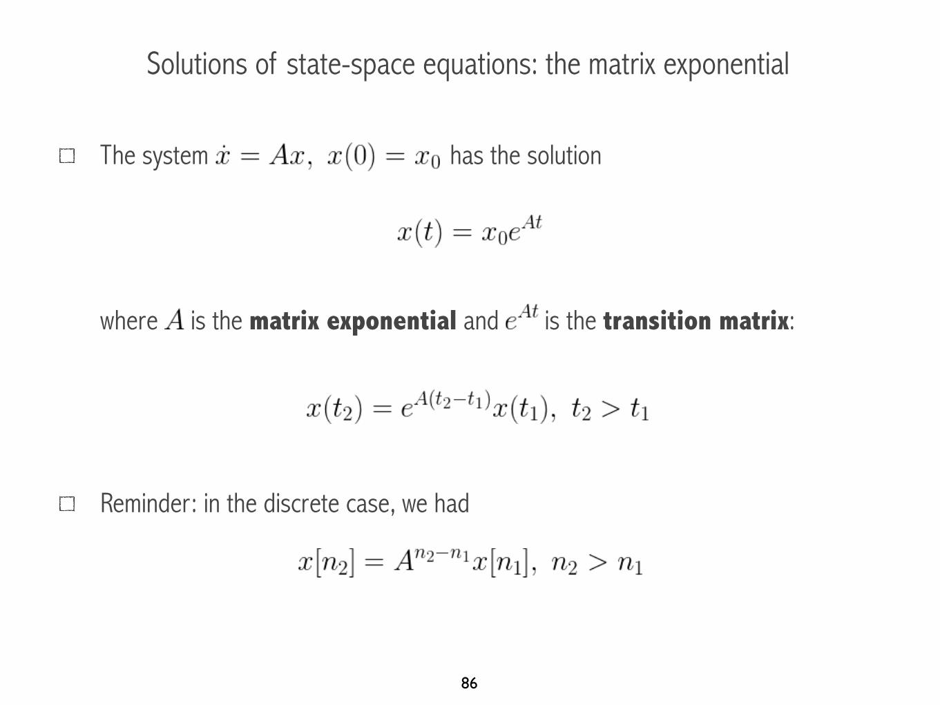
Solutions of state-space equations: the matrix exponential
The system has the solutionwhere is the matrix exponential and is the transition matrix:
Reminder: in the discrete case, we had
86

Solutions of state-space equations
Now, we will try to find the complete solution of the system
We can define such that
The solution of for any input is therefore
87

Solutions of state-space equations: zero-input and zero-state responses
The solution of for any input is
We can use the change of variable , which gives
zero input zero state
88

Computing the matrix exponential: the Jordan form
The solution of the system involves A only if A is the matrix exponential, i.e. it has to respect the properties described earlier.
It means that to find the solution of the state-space equations, the matrix A has to be into a specific form, called the Jordan form (see textbook).
This implies that we have to change the variables of the state-space representation, i.e. make a state-space transformation (same to reach the canonical form).
89
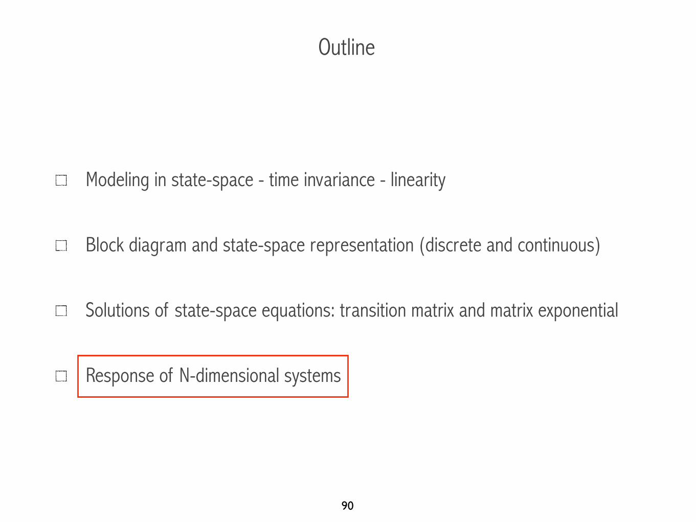
Outline
Modeling in state-space - time invariance - linearity
Block diagram and state-space representation (discrete and continuous)
Solutions of state-space equations: transition matrix and matrix exponential
Response of N-dimensional systems
90

In “state-space”, dynamical systems are modeled using difference equations (discrete domain) or differential equations (continuous domain).
91
is a parameter of the system. A system can have many parameters.a
x =dx
dt
(where )x[n+ 1] = ax[n]
! x[n] = a
n
x = ax
! x(t) = e
at
Discrete domain Continuous domain
a > 0a < 0

In “state-space”, dynamical systems are modeled using difference equations (discrete domain) or differential equations (continuous domain).
92
is a parameter of the system. A system can have many parameters.a
x =dx
dt
(where )x[n+ 1] = ax[n]
! x[n] = a
n
x = ax
! x(t) = e
at
Discrete domain Continuous domain
Systems with more than one variable:
x[n+ 1] = Ax[n]
! x[n] =?
x = Ax
! x(t) =?
Discrete domain Continuous domain
is a square matrix of parameters.A

Response of N-dimensional continuous systems
93
Systems with more than one variable:
x = Ax
! x(t) =?
is a square matrix of parameters. The response will be a sum of exponentials whose coefficients are the eigenvalues of the matrix .A
A
Eigenvalues can be real or complex conjugate pairs. In general:
xi(t) = e
�it = e
(�i+j!i)t
where is the imaginary unit.j
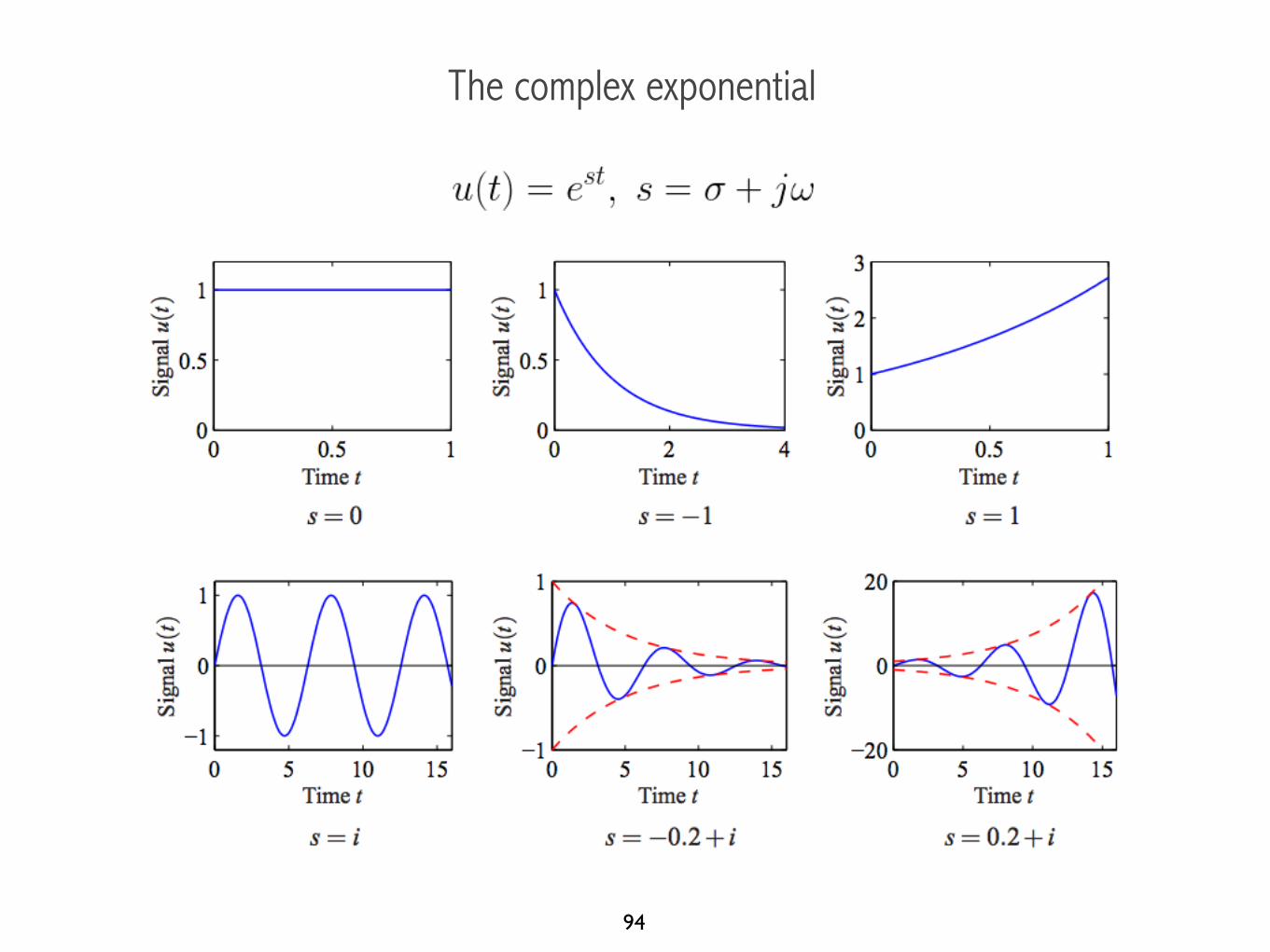
The complex exponential
94

The complex exponential
95
Special case: , giving .

Response of N-dimensional continuous systems
96
Systems with more than one variable:
is a square matrix of parameters. The response will be a sum of exponentials whose coefficients are the eigenvalues of the matrix .A
A
Eigenvalues can be real or complex conjugate pairs. In general:
xi(t) = e
�it = e
(�i+j!i)t
where is the imaginary unit.j
x = Ax
! x(t) =?
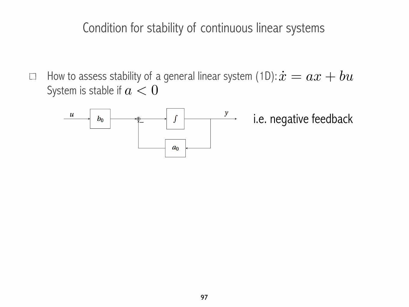
How to assess stability of a general linear system (1D): System is stable if .
How to assess stability of a general linear system (N-D): Multiple state-interactions: what are the feedbacks?N-feedback directions (eigenvectors of matrix ), each having its own amplitude (eigenvalues of ). The system is stable if (all feedbacks negative).
Condition for stability of continuous linear systems
a < 0x = ax+ bu
AA
x = Ax+Bu
R(eig(A)) < 0
i.e. negative feedback
97
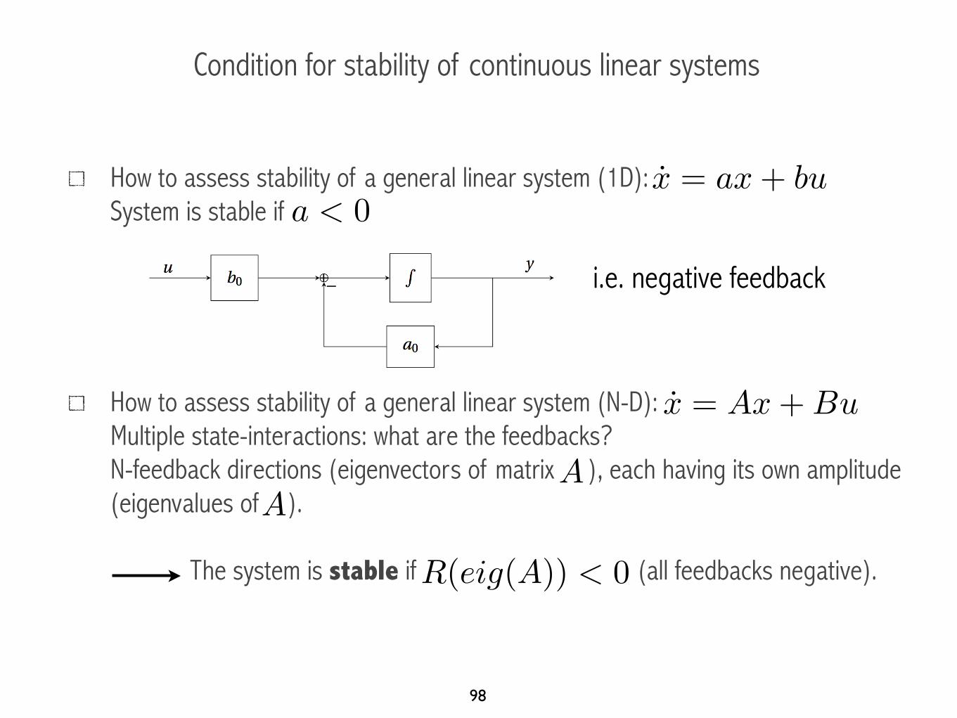
How to assess stability of a general linear system (1D): System is stable if .
How to assess stability of a general linear system (N-D): Multiple state-interactions: what are the feedbacks?N-feedback directions (eigenvectors of matrix ), each having its own amplitude (eigenvalues of ). The system is stable if (all feedbacks negative).
Condition for stability of continuous linear systems
a < 0x = ax+ bu
AA
x = Ax+Bu
R(eig(A)) < 0
i.e. negative feedback
98
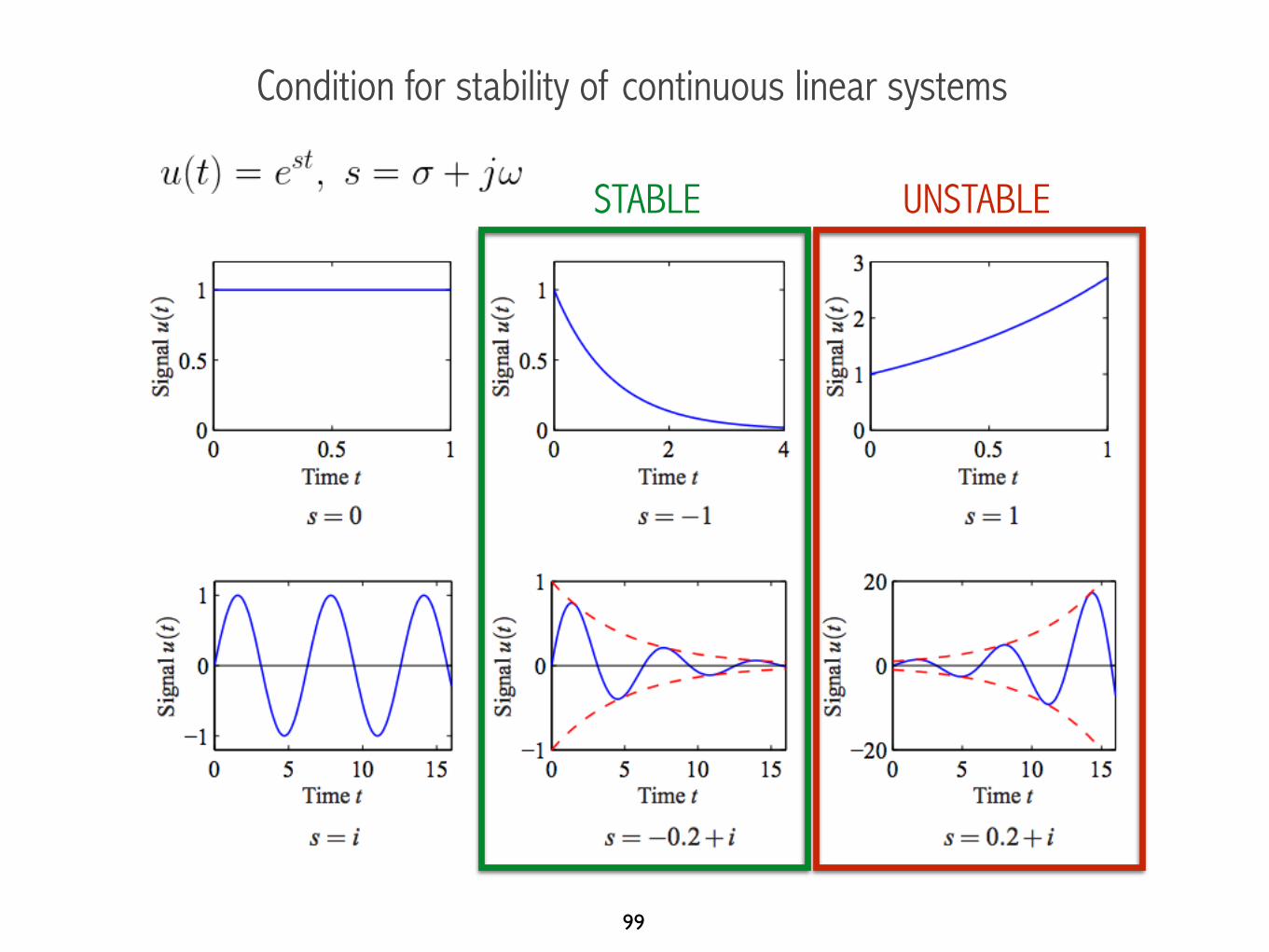
Condition for stability of continuous linear systems
99
STABLE UNSTABLE
Response of N-dimensional discrete systems
100
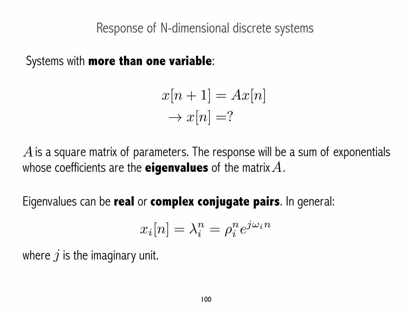
Systems with more than one variable:
is a square matrix of parameters. The response will be a sum of exponentials whose coefficients are the eigenvalues of the matrix .A
A
Eigenvalues can be real or complex conjugate pairs. In general:
where is the imaginary unit.j
x[n+ 1] = Ax[n]
! x[n] =?
xi[n] = �
ni = ⇢
ni e
j!in
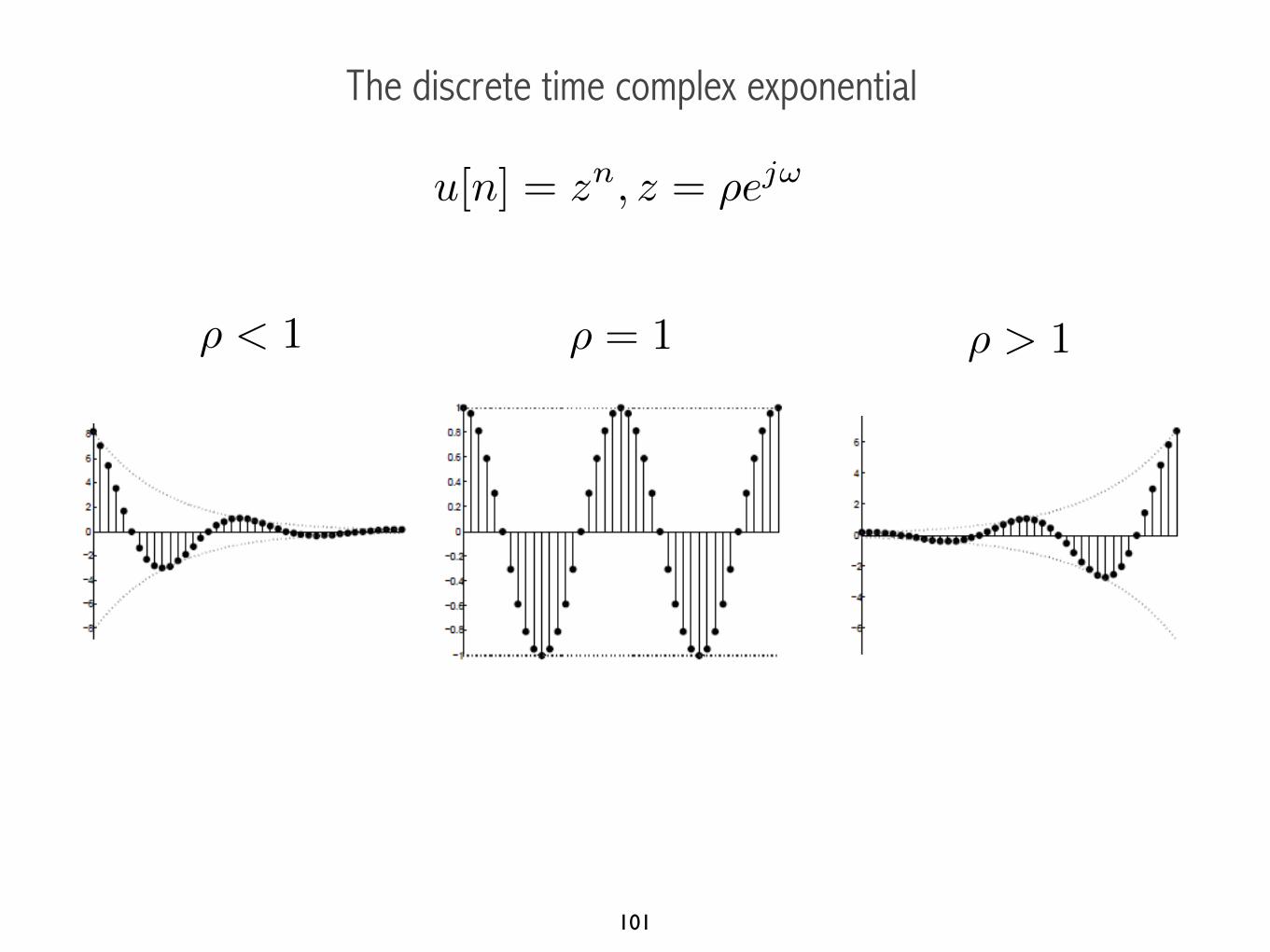
The discrete time complex exponential
101
u[n] = zn, z = ⇢ej!
⇢ < 1 ⇢ = 1 ⇢ > 1

Condition for stability of continuous linear systems
102
u[n] = zn, z = ⇢ej!
⇢ < 1 ⇢ = 1 ⇢ > 1
STABLE UNSTABLE


![Mickelsson’s twisted K-theory invariant and its …math.shinshu-u.ac.jp/~kgomi/papers/mickelsson.pdfMickelsson’s twisted K-theory invariant [18] is an invariant of certain odd](https://static.documents.pub/doc/80x56/5f0881257e708231d42256e4/mickelssonas-twisted-k-theory-invariant-and-its-mathshinshu-uacjpkgomipapers.jpg)


