Srikanth SastryJawaharlal Nehru Centre for

Advanced Scientific ResearchBangalore

SCHOOL ON BIOMOLECULAR SIMULATIONSNovember 6 - 16, 2007

Introduction to simulation methodologies

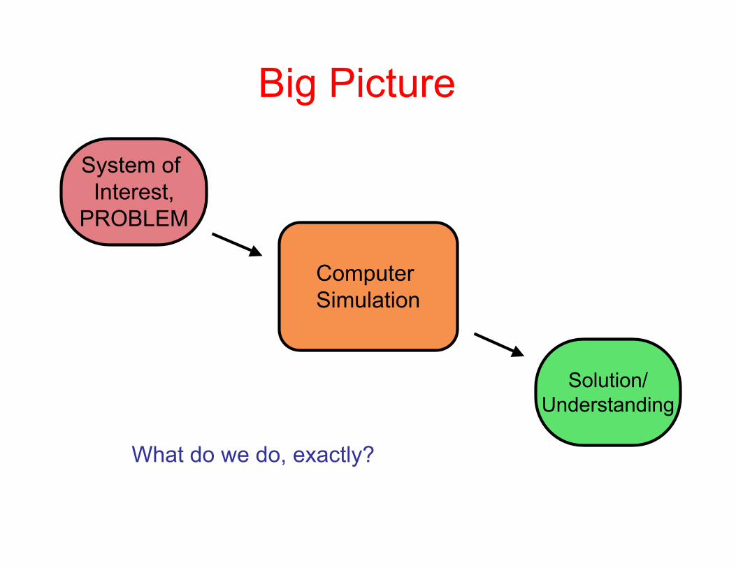
Big Picture

System of Interest,

PROBLEM

Computer Simulation

Solution/Understanding

What do we do, exactly?

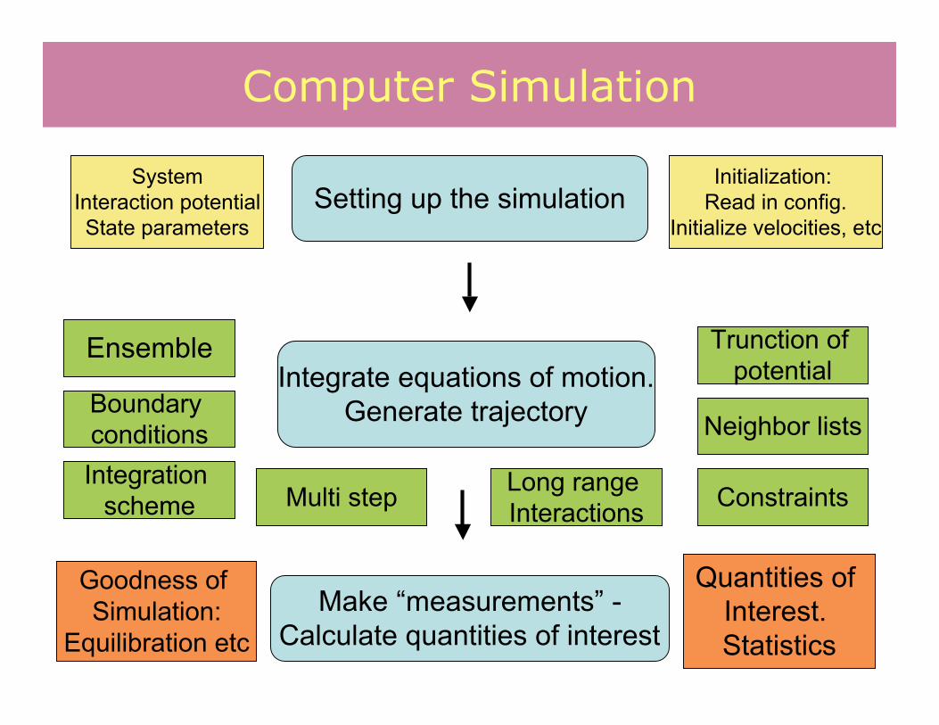
Computer Simulation

Setting up the simulation

Integrate equations of motion.Generate trajectory

Make “measurements” -Calculate quantities of interest

SystemInteraction potentialState parameters

Initialization: Read in config.

Initialize velocities, etc

Ensemble

Boundary conditionsIntegration

scheme

Neighbor lists

ConstraintsMulti step Long range Interactions

Trunction of potential

Goodness of Simulation:

Equilibration etc

Quantities of Interest. Statistics

• Exact or satisfactory statistical mechanical calculation ofproperties of dense systems (liquids, solids, biomolecules)possible only in a limited number of cases.

• Computer simulations (in particular, molecular dynamics) offersmethod to study properties of many particle systemscomputationally.

• Here, we are interested in classical systems, but inclusion ofquantum aspects possible.

• Biomolecular and other “soft” systems -- temperature and entropyplay essential role, though energy optimization is often goodenough.

• Non-equilibrium studies also relevant (eg., protein unfoldingsimulations)

• Integrate equations of motion to obtain trajectory.• Trajectory provides ensemble of configurations to study

equilibrium properties, and permits study of dynamics.

Why simulations?

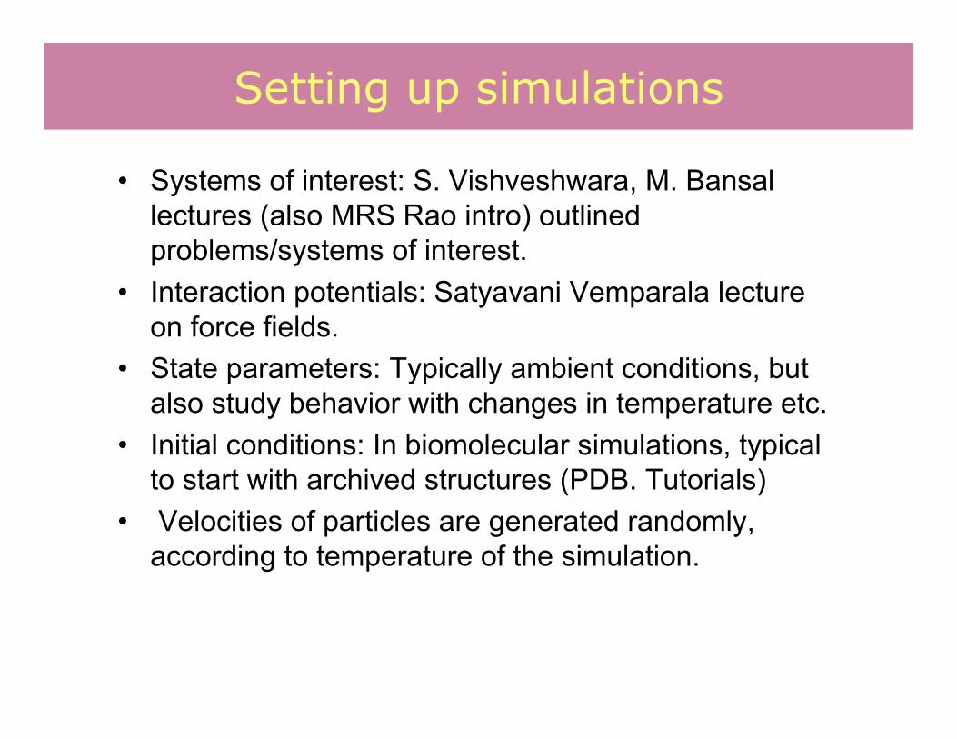
• Systems of interest: S. Vishveshwara, M. Bansallectures (also MRS Rao intro) outlinedproblems/systems of interest.

• Interaction potentials: Satyavani Vemparala lectureon force fields.

• State parameters: Typically ambient conditions, butalso study behavior with changes in temperature etc.

• Initial conditions: In biomolecular simulations, typicalto start with archived structures (PDB. Tutorials)

• Velocities of particles are generated randomly,according to temperature of the simulation.

Setting up simulations

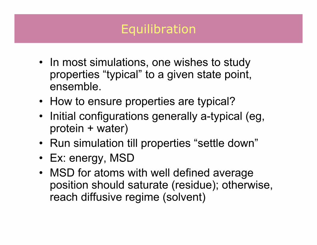
• In most simulations, one wishes to studyproperties “typical” to a given state point,ensemble.

• How to ensure properties are typical?• Initial configurations generally a-typical (eg,

protein + water)• Run simulation till properties “settle down”• Ex: energy, MSD• MSD for atoms with well defined average

position should saturate (residue); otherwise,reach diffusive regime (solvent)

Equilibration

• Typical thermodynamic ensembles of interest: (NVE),(NVT), (NPT)

• Large homogeneous systems: The choice ofensemble doesn’t make a difference for averageproperties (eg, energy), but makes difference tofluctuations (eg, volume fluctuations).

• In the presence of phase transitions, ensemblechoice makes a big difference.

• Integration schemes are harder (NVE) > (NVT) >(NPT).

Integration of equation of motion: Ensemble

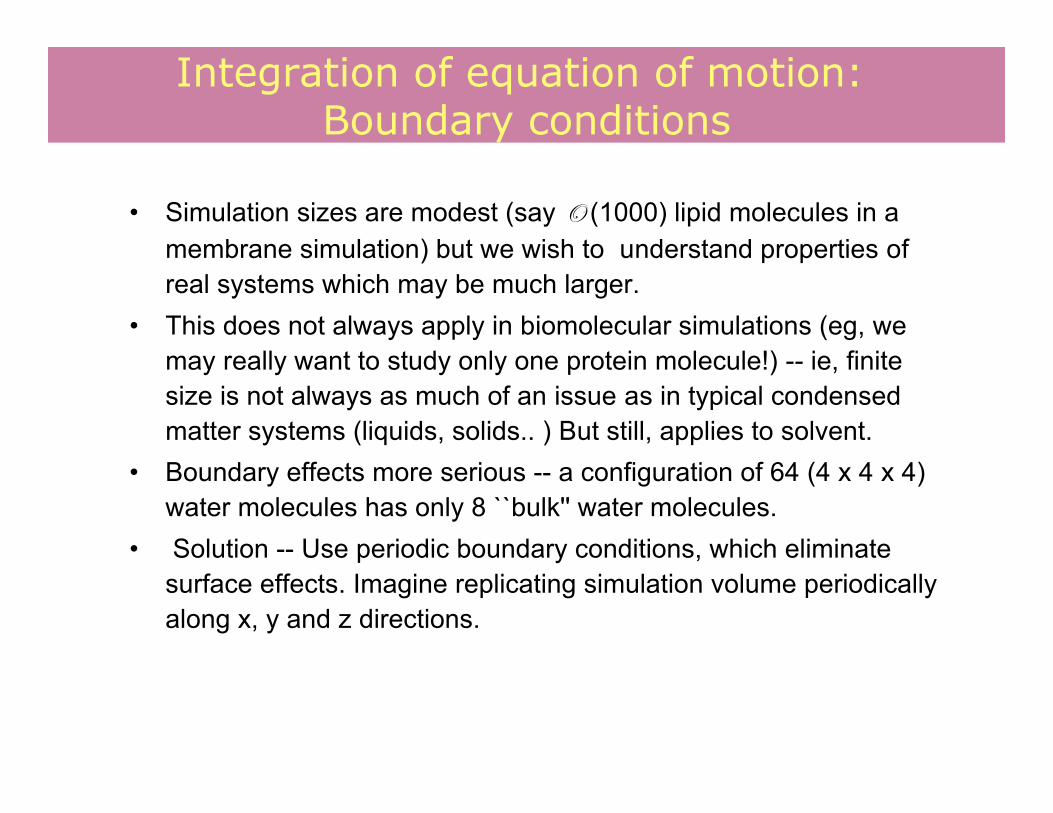
• Simulation sizes are modest (say O (1000) lipid molecules in amembrane simulation) but we wish to understand properties ofreal systems which may be much larger.

• This does not always apply in biomolecular simulations (eg, wemay really want to study only one protein molecule!) -- ie, finitesize is not always as much of an issue as in typical condensedmatter systems (liquids, solids.. ) But still, applies to solvent.

• Boundary effects more serious -- a configuration of 64 (4 x 4 x 4)water molecules has only 8 ``bulk'' water molecules.

• Solution -- Use periodic boundary conditions, which eliminatesurface effects. Imagine replicating simulation volume periodicallyalong x, y and z directions.

Integration of equation of motion: Boundary conditions

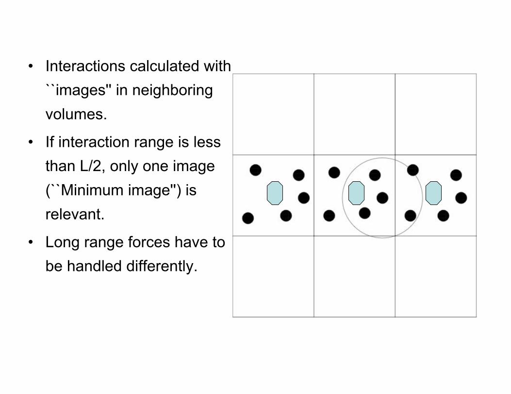
• Interactions calculated with``images'' in neighboringvolumes.

• If interaction range is lessthan L/2, only one image(``Minimum image'') isrelevant.

• Long range forces have tobe handled differently.

• Given an interaction potential, and initialconditions, the equation of motion are:

• Defining a suitable interaction potential for areal system of interest is non-trivial, which will bediscussed in the lecture by Satyavani Vemparala.• The simplest case to consider is integration forconstant energy.• Different cases were covered in S.Balasubrmanian’s lecture.

Integration of equation of motion: Numerical schemes

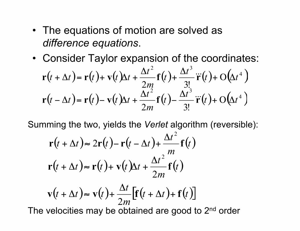
• The equations of motion are solved asdifference equations.

• Consider Taylor expansion of the coordinates:

Summing the two, yields the Verlet algorithm (reversible):

The velocities may be obtained are good to 2nd order

( ) ( ) ( ) ( ) ( ) ( )432

!32tt

tt

m

tttttt !"+

!#

!+!#=!# rfvrr &&&

( ) ( ) ( ) ( ) ( ) ( )432

!32tt

tt

m

tttttt !"+

!+

!+!+=!+ rfvrr &&&

( ) ( ) ( ) ( )tm

tttttt frrr

2

2!

+!""#!+

( ) ( ) ( ) ( )

( ) ( ) ( ) ( )[ ]tttm

tttt

tm

tttttt

ffvv

fvrr

+!+!

+"!+

!+!+"!+

2

2

2

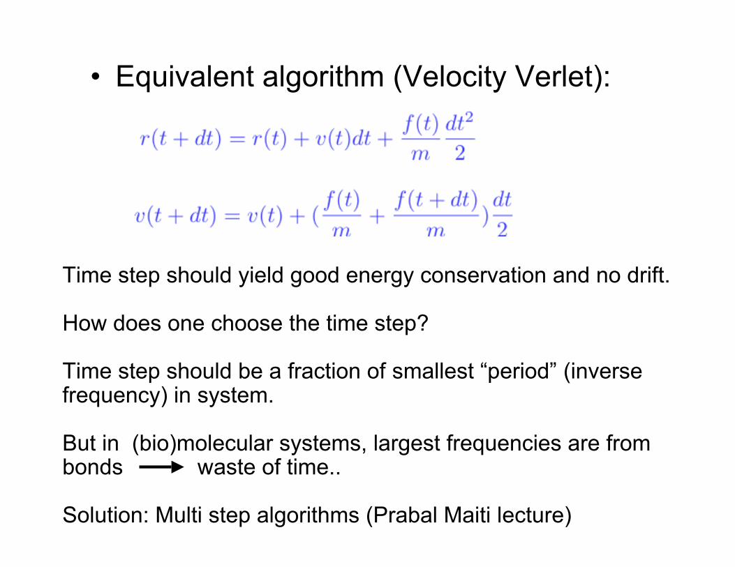
• Equivalent algorithm (Velocity Verlet):

Time step should yield good energy conservation and no drift.

How does one choose the time step?

Time step should be a fraction of smallest “period” (inversefrequency) in system.

But in (bio)molecular systems, largest frequencies are frombonds waste of time..

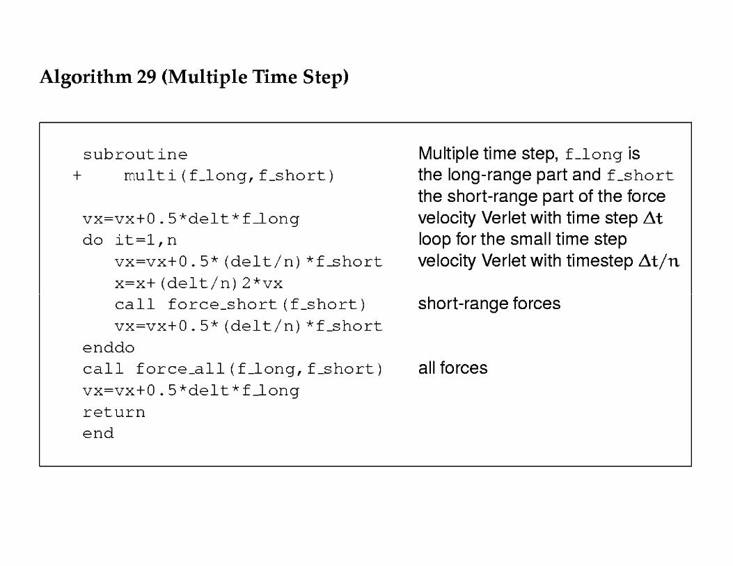
Solution: Multi step algorithms (Prabal Maiti lecture)

Multiple time steps• What to use for stiff potentials:

– Fixed bond-length: constraints (Shake)– Very small time step

Lyaponov instability( ) ( )( )

( ) ( ) ( ) ( ) ( )( )1

10

0 , 0

0 , 0 , , 0 , 0 , 0

10

N N

N

j i N! !

! "

+ "

=

r p

r p p p pL L

However, equilibrium average, as well as

dynamical properties are not affected by this.

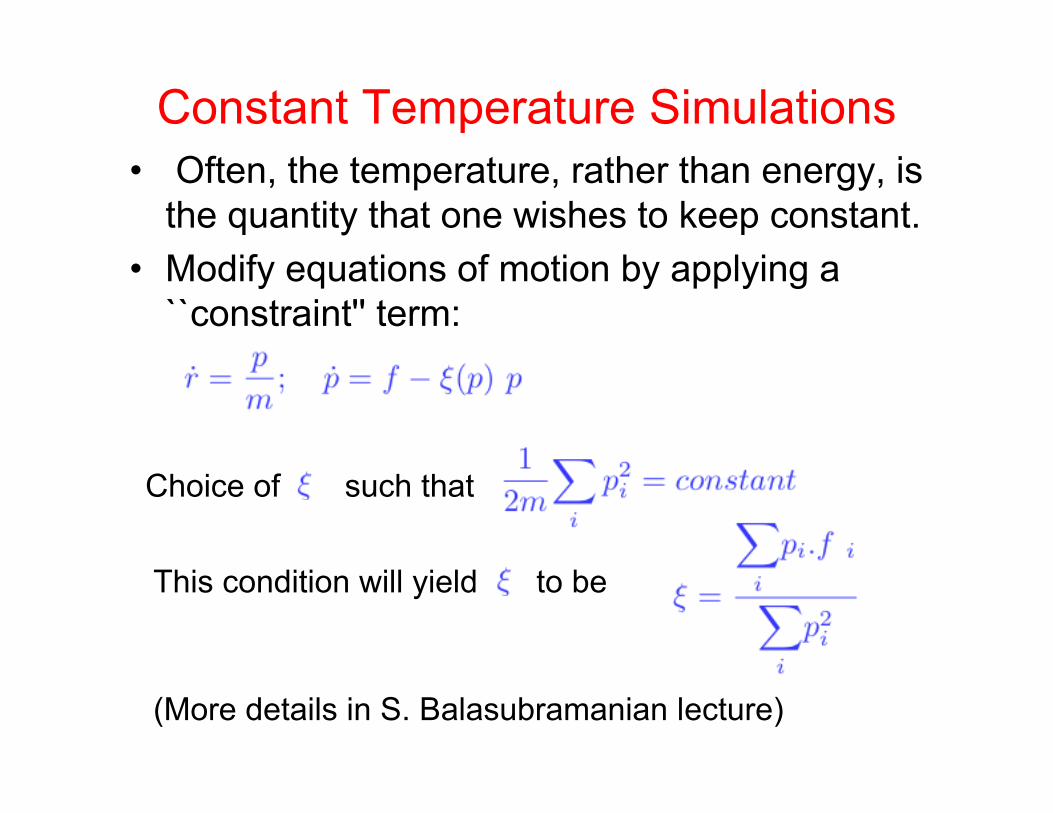
Constant Temperature Simulations• Often, the temperature, rather than energy, is

the quantity that one wishes to keep constant.• Modify equations of motion by applying a

``constraint'' term:

Choice of such that

This condition will yield to be

(More details in S. Balasubramanian lecture)

Neighbor Lists• During the course of the

simulation, interactions have tobe calculated between all pairsof particles, which naivelyscales at N2.

• For finite range interactions,however, only a few neighborsare relevant.

• Force calculation can be O(N)if neighbors are kept track of.

• Neighbor lists -- For cutoff rc,keep track of neighbors withinre > rc.

• Update when maximumdisplacement > |re- rc| Verlet Neighbor List

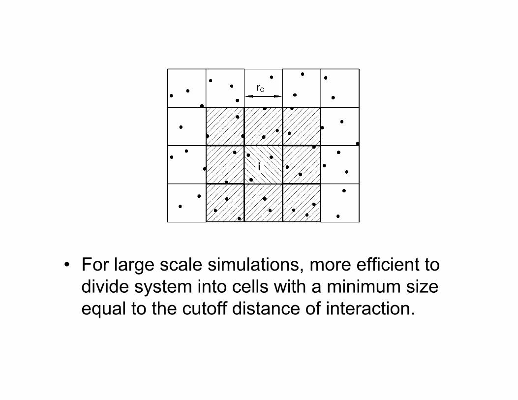
• For large scale simulations, more efficient todivide system into cells with a minimum sizeequal to the cutoff distance of interaction.

Truncation of interaction potential

( )!!"

#

$$%

&'(

)*+

,-'

(

)*+

,=

612

4rr

ruLJ ..

/

( )( )

!"#

>

$=

c

c

LJ

rr

rrruru

0

( )( ) ( )

!"#

>

$%=

c

cc

LJLJ

rr

rrrururu

0

•The truncated and shifted Lennard-Jones potential

•The truncated Lennard-Jones potential

•The Lennard-Jones potential But care must be taken to correct for truncation ifone wishes to study the

full potential.

Long Range Interactions

• For interactions such as Couloumbinteraction, one cannot truncate the potential.

• Ewald sum: Given a distribution of pointcharges, equivalent distribution is (pointcharges + Gaussian charge distribution withopposite total charge) - Gaussian distributionwith same sign.

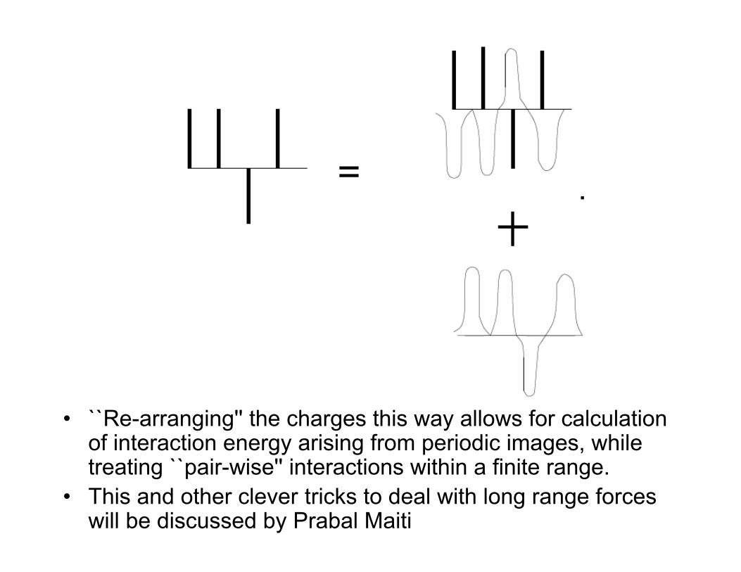
• ``Re-arranging'' the charges this way allows for calculationof interaction energy arising from periodic images, whiletreating ``pair-wise'' interactions within a finite range.

• This and other clever tricks to deal with long range forceswill be discussed by Prabal Maiti

Molecular SystemsH

HO

Further details in the next lecture.