15
Introduction to System Dynamics Prof. Davide Manca – Politecnico di Milano Dynamics and Control of Chemical Processes Solution to Lab #1 SE1

© Davide Manca – Dynamics and Control of Chemical Processes – Master Degree in ChemEng – Politecnico di Milano 1SE1—
Introduction to System
Dynamics
Prof. Davide Manca – Politecnico di Milano
Dynamics and Control of Chemical Processes
Solution to Lab #1
SE1

© Davide Manca – Dynamics and Control of Chemical Processes – Master Degree in ChemEng – Politecnico di Milano 2SE1—
E1 – Dynamics of a biological system
A biological process is run in a batch reactor where the biomass (B) grows by feeding on
the substrate (S). The material balances for the two species are:
1
2
13
2
k BSdB
dt k S
k BSdSk
dt k S
-1
1 0.5 hk 7 3
2 10 kmol mk 3 0.6k With:
3
3
0 0.03 kmol m
0 4.5 kmol m
B
S
The initial conditions are:

© Davide Manca – Dynamics and Control of Chemical Processes – Master Degree in ChemEng – Politecnico di Milano 3SE1—
E1 - Aim
• Determine the dynamic evolution of both biomass and substrate over a time
interval of 15 h.
• Use Matlab to solve the ordinary differential equations (ODE) system: (i) with
the standard precision (i.e. by default) for both absolute and relative tolerances.
(ii) Modify those tolerances with a relative tolerance of 1.e-8 and an absolute
one of 1.e-12. Compare the two dynamics and provide a comment about
them.

© Davide Manca – Dynamics and Control of Chemical Processes – Master Degree in ChemEng – Politecnico di Milano 4SE1—
Integration of ODE in MATLAB
To integrate the ordinary differential system one can use the functions
implemented in MATLAB:
ode15s: for the integration of stiff systems
[t,y] = ode15s(@(t,y)myFun(t,y,params),tSpan,y0,options)
ode45: for the integration of non-stiff systems.
[t,y] = ode45(@(t,y)myFun(t,y,params),tSpan,y0,options)

© Davide Manca – Dynamics and Control of Chemical Processes – Master Degree in ChemEng – Politecnico di Milano 5SE1—
Integration of ODE in MATLAB
• Where:
t = time
y = the dependent variables matrix (each column represents a variable)
myFun = name of the ODE function
tSpan = integration time span [tMin tMax]
y0 = vector of initial conditions, e.g., [B0 S0]
params = list of optional parameters for the solution of the differential system
(e.g., k1, k2, k3) [params vector must however be always present even if no
specific parameters are used)
options = options for the integrator
options = odeset('RelTol',1E-8,'AbsTol',1E-12)
© Davide Manca – Dynamics and Control of Chemical Processes – Master Degree in ChemEng – Politecnico di Milano 6SE1—
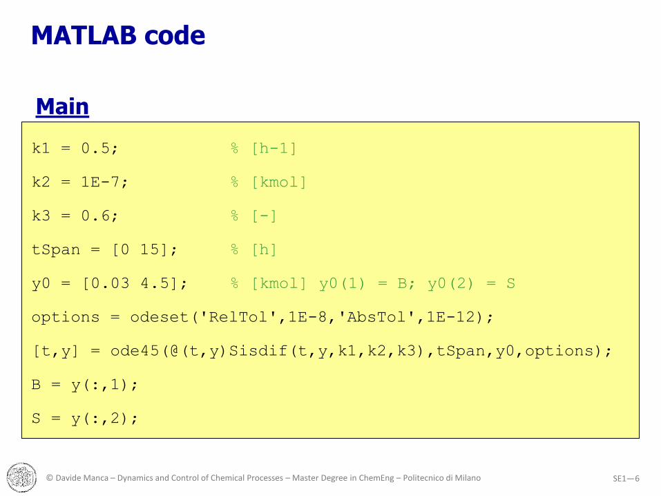
MATLAB code
k1 = 0.5; % [h-1]
k2 = 1E-7; % [kmol]
k3 = 0.6; % [-]
tSpan = [0 15]; % [h]
y0 = [0.03 4.5]; % [kmol] y0(1) = B; y0(2) = S
options = odeset('RelTol',1E-8,'AbsTol',1E-12);
[t,y] = ode45(@(t,y)Sisdif(t,y,k1,k2,k3),tSpan,y0,options);
B = y(:,1);
S = y(:,2);
Main

© Davide Manca – Dynamics and Control of Chemical Processes – Master Degree in ChemEng – Politecnico di Milano 7SE1—
Sisdif
function dy = Sisdif(t,y,k1,k2,k3)
dy = zeros(2,1); % column vector
B = y(1);
S = y(2);
dy(1) = k1*B*S / (S + k2);
dy(2) = - k3 * dy(1);
MATLAB code

© Davide Manca – Dynamics and Control of Chemical Processes – Master Degree in ChemEng – Politecnico di Milano 8SE1—
figure(1)
plot(t,B,'r',t,S,'b','LineWidth',3)
set(gca,'FontSize',18)
legend('Biomass','Substrate',2)
xlabel('Time [h]')
ylabel('Mass [kmol]')
title('Dynamics of substrate and biomass')
grid off
saveas(figure(1),'Biological System.emf')
Results display
Advice: do not use the extension .fig
MATLAB code

© Davide Manca – Dynamics and Control of Chemical Processes – Master Degree in ChemEng – Politecnico di Milano 9SE1—
Dynamics of a biological system (1)
Physically impossible
0 5 10 15-40
-20
0
20
40
60
Time [h]
Mole
[km
ol]
Dynamics of substrate and biomass
Biomass
Substrate

© Davide Manca – Dynamics and Control of Chemical Processes – Master Degree in ChemEng – Politecnico di Milano 10SE1—
0 5 10 15-2
0
2
4
6
8
Time [h]
Mole
[km
ol]
Dynamics of substrate and biomass
Biomass
Substrate
Dynamics of a biological system (2)

© Davide Manca – Dynamics and Control of Chemical Processes – Master Degree in ChemEng – Politecnico di Milano 11SE1—
E2 – Dynamics of a perfectly mixed tank
An intermediate tank is perfectly mixed (i.e. it is a continuously stirred tank, aka CST)
and heated. Determine the dynamics of the outlet temperature when there is a step
disturbance of 30 °C in the inlet temperature, with:
• Heating power:
• Inlet flowrate:
• CST mass holdup:
• Specific molar heat:
• Initial inlet temperature:
1 MWQ
8 kmol siF
100 kmolm
2.5 kJ kmolKcp
300 KiT

© Davide Manca – Dynamics and Control of Chemical Processes – Master Degree in ChemEng – Politecnico di Milano 12SE1—
Modelling of the system
, i iF T , o oF T
Q
i o
p o p o i
F F
dTmc F c T T Q
dt
Energy balance:
Mass balance:

© Davide Manca – Dynamics and Control of Chemical Processes – Master Degree in ChemEng – Politecnico di Milano 13SE1—
Results
0 100 200 300300
320
340
360
380
400
Time [s]
Tem
pera
ture
[K
]
Dynamics of CSTR Temperature
© Davide Manca – Dynamics and Control of Chemical Processes – Master Degree in ChemEng – Politecnico di Milano 14SE1—
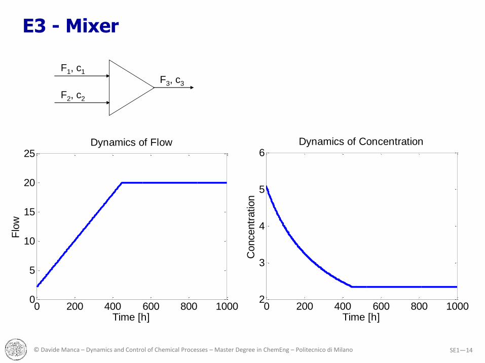
E3 - Mixer
F1, c1
F2, c2
F3, c3
0 200 400 600 800 10000
5
10
15
20
25
Time [h]
Flo
w
Dynamics of Flow
0 200 400 600 800 10002
3
4
5
6
Time [h]
Concentr
ation
Dynamics of Concentration

© Davide Manca – Dynamics and Control of Chemical Processes – Master Degree in ChemEng – Politecnico di Milano 15SE1—
E4 –Runaway dynamics
0 5 10 15 200
0.2
0.4
0.6
0.8
1
1.2
1.4
Time [-]
Concentr
ation
Concentration profile
0 5 10 15 200
5
10
15
20
Time [-]
Tem
pera
ture
Temperature profile


