23
Introduction to the Technique of Electron Spin Resonance (ESR) Spectroscopy Physics Laboratory Course Dr . B. Si movi ˇ c April 20, 2004
| Date post: | 07-Apr-2018 |
| Category: |
Documents |
| Upload: | jonathan-robert-kraus-outofmudproductions |
| View: | 230 times |
| Download: | 0 times |
8/4/2019 Introduction to the Technique of Electron Spin Resonance (ESR) Spectroscopy
http://slidepdf.com/reader/full/introduction-to-the-technique-of-electron-spin-resonance-esr-spectroscopy 1/23
Introduction to the Technique of Electron Spin Resonance (ESR)
Spectroscopy
Physics Laboratory Course
Dr. B. Simovic
April 20, 2004
8/4/2019 Introduction to the Technique of Electron Spin Resonance (ESR) Spectroscopy
http://slidepdf.com/reader/full/introduction-to-the-technique-of-electron-spin-resonance-esr-spectroscopy 2/23
Abstract
Electron spin resonance (esr) spectroscopy deals with the in-
teraction of electromagnetic radiation with the intrinsic mag-
netic moment of electrons arising from their spin. It has found
applications in a wide range of different fields spanning fromchemistry and biology to the novel and stimulating areas of
quantum computation and ”single spin” detection. This labora-
tory course provides a basic introduction to esr. It is intended
to motivate students eager to learn about experimental as-
pects of spectroscopy.
8/4/2019 Introduction to the Technique of Electron Spin Resonance (ESR) Spectroscopy
http://slidepdf.com/reader/full/introduction-to-the-technique-of-electron-spin-resonance-esr-spectroscopy 3/23
Chapter 1
Introduction
1.1 What is ESR?
The phenomenon of electron spin resonance spectroscopy can be explained by
considering the behavior of a free electron. According to quantum theory the
electron has a spin which can be understood as an angular momentum leading
to a magnetic moment. Consequently, the negative charge that the electron
carries is also spinning and constitutes a circulating electric current. The
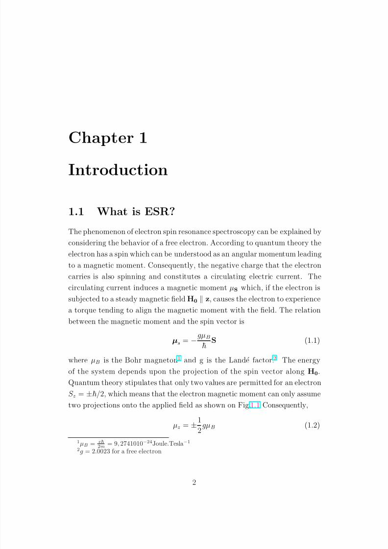
circulating current induces a magnetic moment µS which, if the electron issubjected to a steady magnetic field H0 z, causes the electron to experience
a torque tending to align the magnetic moment with the field. The relation
between the magnetic moment and the spin vector is
µs = −gµB
S (1.1)
where µB is the Bohr magneton1 and g is the Lande factor.2 The energy
of the system depends upon the projection of the spin vector along H0.
Quantum theory stipulates that only two values are permitted for an electronS z = ±/2, which means that the electron magnetic moment can only assume
two projections onto the applied field as shown on Fig.1.1 Consequently,
µz = ±1
2gµB (1.2)
1µB = e
2m= 9, 2741010−24Joule.Tesla−1
2g = 2.0023 for a free electron
2
8/4/2019 Introduction to the Technique of Electron Spin Resonance (ESR) Spectroscopy
http://slidepdf.com/reader/full/introduction-to-the-technique-of-electron-spin-resonance-esr-spectroscopy 4/23
H0
E + = ½ gµµµµB/
E - = - ½ gµµµµB/
¡
ω0
(a) (b)
µµµµ
e-
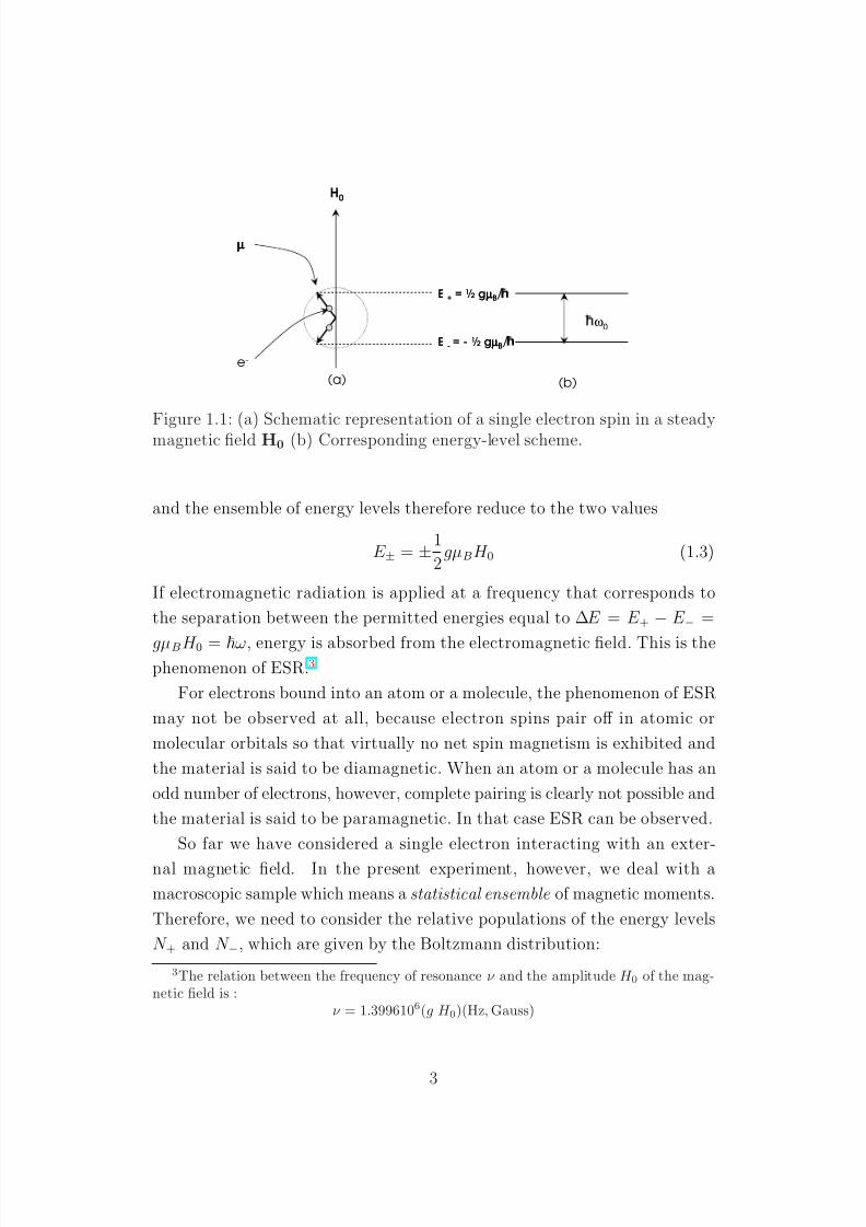
Figure 1.1: (a) Schematic representation of a single electron spin in a steadymagnetic field H0 (b) Corresponding energy-level scheme.
and the ensemble of energy levels therefore reduce to the two values
E ± = ±1
2gµBH 0 (1.3)
If electromagnetic radiation is applied at a frequency that corresponds to
the separation between the permitted energies equal to ∆E = E + − E − =
gµBH 0 = ω, energy is absorbed from the electromagnetic field. This is thephenomenon of ESR.3
For electrons bound into an atom or a molecule, the phenomenon of ESR
may not be observed at all, because electron spins pair off in atomic or
molecular orbitals so that virtually no net spin magnetism is exhibited and
the material is said to be diamagnetic. When an atom or a molecule has an
odd number of electrons, however, complete pairing is clearly not possible and
the material is said to be paramagnetic. In that case ESR can be observed.
So far we have considered a single electron interacting with an exter-
nal magnetic field. In the present experiment, however, we deal with a
macroscopic sample which means a statistical ensemble of magnetic moments.
Therefore, we need to consider the relative populations of the energy levels
N + and N −, which are given by the Boltzmann distribution:
3The relation between the frequency of resonance ν and the amplitude H 0 of the mag-netic field is :
ν = 1.3996106(g H 0)(Hz, Gauss)
3
8/4/2019 Introduction to the Technique of Electron Spin Resonance (ESR) Spectroscopy
http://slidepdf.com/reader/full/introduction-to-the-technique-of-electron-spin-resonance-esr-spectroscopy 5/23
Sz =1/2
Sz = -1/2
-3/2
-5/2
-1/2
1/2
3/2
5/2
3/2
5/2
1/2
-1/2
-3/2
-5/2
Iz
Mn 2+ ion I=5/2
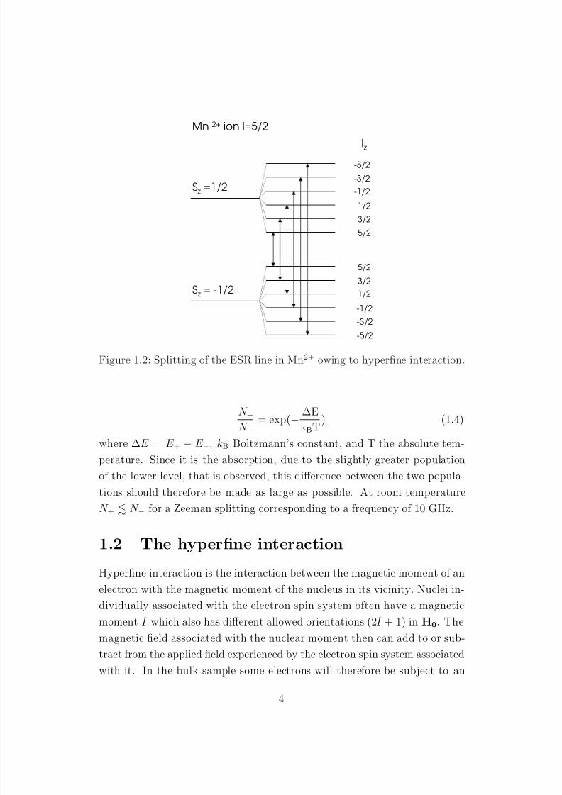
Figure 1.2: Splitting of the ESR line in Mn2+ owing to hyperfine interaction.
N +
N −= exp(− ∆EkBT) (1.4)
where ∆E = E + − E −, kB Boltzmann’s constant, and T the absolute tem-
perature. Since it is the absorption, due to the slightly greater population
of the lower level, that is observed, this difference between the two popula-
tions should therefore be made as large as possible. At room temperature
N + N − for a Zeeman splitting corresponding to a frequency of 10 GHz.
1.2 The hyperfine interaction
Hyperfine interaction is the interaction between the magnetic moment of an
electron with the magnetic moment of the nucleus in its vicinity. Nuclei in-
dividually associated with the electron spin system often have a magnetic
moment I which also has different allowed orientations (2I + 1) in H0. The
magnetic field associated with the nuclear moment then can add to or sub-
tract from the applied field experienced by the electron spin system associated
with it. In the bulk sample some electrons will therefore be subject to an
4
8/4/2019 Introduction to the Technique of Electron Spin Resonance (ESR) Spectroscopy
http://slidepdf.com/reader/full/introduction-to-the-technique-of-electron-spin-resonance-esr-spectroscopy 6/23
N N
NO2
NO2
NO2
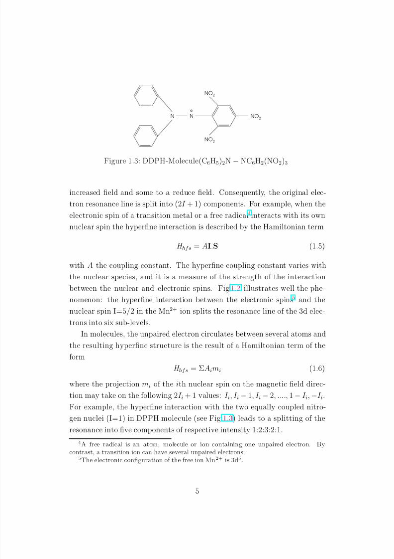
Figure 1.3: DDPH-Molecule(C6H5)2N − NC6H2(NO2)3
increased field and some to a reduce field. Consequently, the original elec-tron resonance line is split into (2I + 1) components. For example, when the
electronic spin of a transition metal or a free radical4interacts with its own
nuclear spin the hyperfine interaction is described by the Hamiltonian term
H hfs = AI.S (1.5)
with A the coupling constant. The hyperfine coupling constant varies with
the nuclear species, and it is a measure of the strength of the interaction
between the nuclear and electronic spins. Fig.1.2 illustrates well the phe-
nomenon: the hyperfine interaction between the electronic spins5 and the
nuclear spin I=5/2 in the Mn2+ ion splits the resonance line of the 3d elec-
trons into six sub-levels.
In molecules, the unpaired electron circulates between several atoms and
the resulting hyperfine structure is the result of a Hamiltonian term of the
form
H hfs = ΣAimi (1.6)
where the projection mi of the ith nuclear spin on the magnetic field direc-
tion may take on the following 2I i + 1 values: I i, I i− 1, I i− 2, ...., 1− I i,−I i.
For example, the hyperfine interaction with the two equally coupled nitro-
gen nuclei (I=1) in DPPH molecule (see Fig.1.3) leads to a splitting of the
resonance into five components of respective intensity 1:2:3:2:1.
4A free radical is an atom, molecule or ion containing one unpaired electron. Bycontrast, a transition ion can have several unpaired electrons.
5The electronic configuration of the free ion Mn2+ is 3d5.
5
8/4/2019 Introduction to the Technique of Electron Spin Resonance (ESR) Spectroscopy
http://slidepdf.com/reader/full/introduction-to-the-technique-of-electron-spin-resonance-esr-spectroscopy 7/23
1.3 The dipole-dipole interaction
For a large concentration of electronic spins, the electronic magnetic moments
also interact appreciably with each other, and this can alter considerably the
ESR spectra. The interaction is mediated by the dipolar field associated with
the magnetic moment µS
H(r) =µ04π
1
r3(−µS +
3(µS .r)r
r2) (1.7)
Combining equation1.2 and 1.3, we see that the energy of dipole-dipole in-
teraction between two adjacent electrons distant of r lays between E dd and−E dd with
E dd =µ08πg2µ2B
1
r3(1.8)
The dipolar interaction induces therefore a broadening of the resonance line,
which increases with the concentration of dipole moments.
6
8/4/2019 Introduction to the Technique of Electron Spin Resonance (ESR) Spectroscopy
http://slidepdf.com/reader/full/introduction-to-the-technique-of-electron-spin-resonance-esr-spectroscopy 8/23
Chapter 2
ESR spectrometer
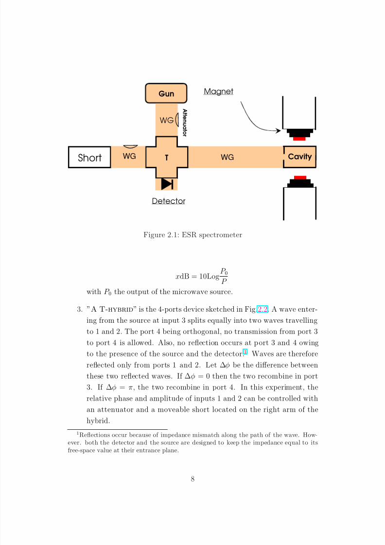
We need four essential components to build an ESR spectrometer:
• A monochromatic microwave source
• A waveguide for guiding the microwave power to the sample
• A cavity designed to ensure a proper coupling between the sample and
the incoming wave.
• A detector for microwave power to detect the response of the sample
to microwave irradiation.
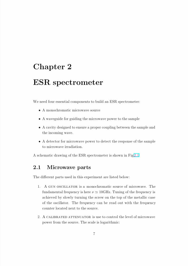
A schematic drawing of the ESR spectrometer is shown in Fig.2.1
2.1 Microwave parts
The different parts used in this experiment are listed below:
1. A gun oscillator is a monochromatic source of microwave. Thefundamental frequency is here ν 10GHz. Tuning of the frequency is
achieved by slowly turning the screw on the top of the metallic case
of the oscillator. The frequency can be read out with the frequency
counter located next to the source.
2. A calibrated attenuator is use to control the level of microwave
power from the source. The scale is logarithmic:
7
8/4/2019 Introduction to the Technique of Electron Spin Resonance (ESR) Spectroscopy
http://slidepdf.com/reader/full/introduction-to-the-technique-of-electron-spin-resonance-esr-spectroscopy 9/23
Gun
T
WG
At t en u at or
Short WG
Detector
CavityWG
Magnet
Figure 2.1: ESR spectrometer
xdB = 10LogP 0P
with P 0 the output of the microwave source.
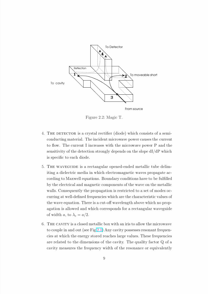
3. ”A T-hybrid” is the 4-ports device sketched in Fig.2.2. A wave enter-
ing from the source at input 3 splits equally into two waves travelling
to 1 and 2. The port 4 being orthogonal, no transmission from port 3
to port 4 is allowed. Also, no reflection occurs at port 3 and 4 owing
to the presence of the source and the detector.1 Waves are therefore
reflected only from ports 1 and 2. Let ∆φ be the difference between
these two reflected waves. If ∆φ = 0 then the two recombine in port
3. If ∆φ = π, the two recombine in port 4. In this experiment, the
relative phase and amplitude of inputs 1 and 2 can be controlled with
an attenuator and a moveable short located on the right arm of the
hybrid.
1Reflections occur because of impedance mismatch along the path of the wave. How-ever. both the detector and the source are designed to keep the impedance equal to itsfree-space value at their entrance plane.
8
8/4/2019 Introduction to the Technique of Electron Spin Resonance (ESR) Spectroscopy
http://slidepdf.com/reader/full/introduction-to-the-technique-of-electron-spin-resonance-esr-spectroscopy 10/23
To cavity
¡
¡¡
¡
¢
¢¢
¢
Reflection
To Detector
To moveable short
From source
£
££
£
Figure 2.2: Magic T.
4. The detector is a crystal rectifier (diode) which consists of a semi-
conducting material. The incident microwave power causes the current
to flow. The current I increases with the microwave power P and the
sensitivity of the detection strongly depends on the slope dI/dP which
is specific to each diode.
5. The waveguide is a rectangular opened-ended metallic tube delim-
iting a dielectric media in which electromagnetic waves propagate ac-
cording to Maxwell equations. Boundary conditions have to be fulfilled
by the electrical and magnetic components of the wave on the metallic
walls. Consequently the propagation is restricted to a set of modes oc-
curring at well-defined frequencies which are the characteristic values of
the wave equation. There is a cut-off wavelength above which no prop-
agation is allowed and which corresponds for a rectangular waveguide
of width a, to λc = a/2.
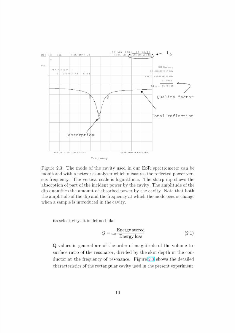
6. The cavity is a closed metallic box with an iris to allow the microwave
to couple in and out (see Fig.2.1) Any cavity possesses resonant frequen-
cies at which the energy stored reaches large values. These frequencies
are related to the dimensions of the cavity. The quality factor Q of a
cavity measures the frequency width of the resonance or equivalently
9
8/4/2019 Introduction to the Technique of Electron Spin Resonance (ESR) Spectroscopy
http://slidepdf.com/reader/full/introduction-to-the-technique-of-electron-spin-resonance-esr-spectroscopy 11/23
Frequency
Total reflection
Absorption
Quality factor
f0
Figure 2.3: The mode of the cavity used in our ESR spectrometer can be
monitored with a network-analyzer which measures the reflected power ver-sus frequency. The vertical scale is logarithmic. The sharp dip shows theabsorption of part of the incident power by the cavity. The amplitude of thedip quantifies the amount of absorbed power by the cavity. Note that boththe amplitude of the dip and the frequency at which the mode occurs changewhen a sample is introduced in the cavity.
its selectivity. It is defined like
Q = ω0Energy stored
Energy loss (2.1)
Q-values in general are of the order of magnitude of the volume-to-
surface ratio of the resonator, divided by the skin depth in the con-
ductor at the frequency of resonance. Figure 2.3 shows the detailed
characteristics of the rectangular cavity used in the present experiment.
10
8/4/2019 Introduction to the Technique of Electron Spin Resonance (ESR) Spectroscopy
http://slidepdf.com/reader/full/introduction-to-the-technique-of-electron-spin-resonance-esr-spectroscopy 12/23
2.2 Electronic equipments
1. An oscilloscope with its X and Y channels.
2. A plotter also with its X and Y channels.
3. The pre-amplifier amplifies in two successive steps: a first dc am-
plification and an ac amplification through a 115 Hz-bandpass filter.
Beware of not saturating the dc stage of amplification.
4. The GUN power supply delivers 15V.
5. A Hall-probe measures the static magnetic field. As indicated by its
name, the principle of operation is based on the Hall-effect. The probe
should therefore be positioned vertically relative to the magnetic field
in order to get the maximum sensitivity. Be careful when manipulating
the probe. It is indeed fragile and expensive.
6. The gaussmeter converts the voltage measured from the Hall-probe
into a value of magnetic field (the maximum deviation corresponds to
1V).
7. The two sets of coils I and II generate the static magnetic field
H0 and the small modulating field Hm respectively.
8. The magnet power supply supplies the current to the pair of coils I
which produces the static field. It is controlled by the ramp-generator.
The current is extremely stable in order to avoid spurious noise that
could interfere with the measurement.
9. The low frequency oscillator creates a sinusoidal current atthe frequency of 115 Hz in the second pair of coil (II). This produces
the field Hm and provides the external reference signal for the lock-in
amplifier
10. The ramp-generator produces a ramp of magnetic field by varying
continuously the current in the pair of coils I. The voltage output of the
ramp can be connected to the X-channel of the plotter if the variation
11
8/4/2019 Introduction to the Technique of Electron Spin Resonance (ESR) Spectroscopy
http://slidepdf.com/reader/full/introduction-to-the-technique-of-electron-spin-resonance-esr-spectroscopy 13/23
of static fields are too small to be accurately read from the gaussmeter.
For larger amplitude of change, the analogue output of the gaussmeter
can be converted to a digital signal and sent to the X-channel of the
plotter.
11. The lock-in amplifier amplifies signals at frequencies close to the
frequency of a reference signal. More details concerning the principle
of operation of a lock-in are given in the following section. Here we
emphasize that the reference signal should come from the low frequency
oscillator. Be careful to connect the 115Hz signal to the proper input
of the lock-in amplifier.
12
8/4/2019 Introduction to the Technique of Electron Spin Resonance (ESR) Spectroscopy
http://slidepdf.com/reader/full/introduction-to-the-technique-of-electron-spin-resonance-esr-spectroscopy 14/23
Chapter 3
Detection scheme
3.1 ESR signal
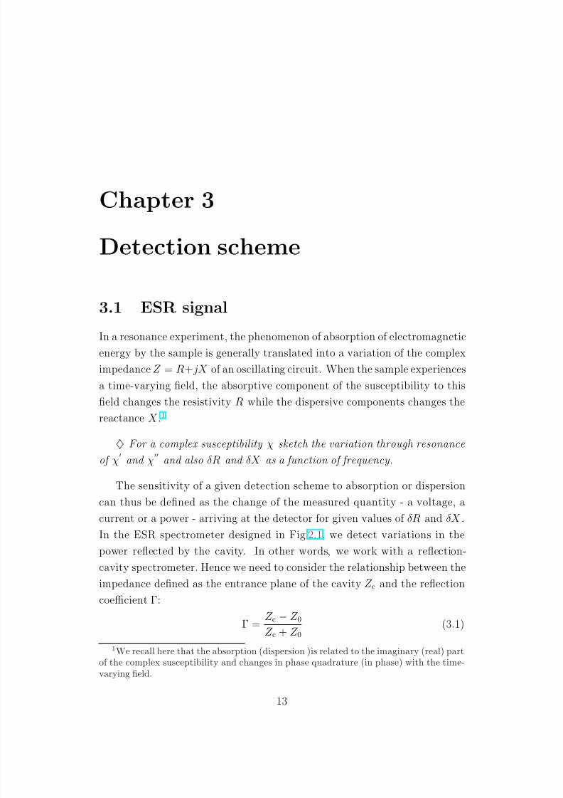
In a resonance experiment, the phenomenon of absorption of electromagnetic
energy by the sample is generally translated into a variation of the complex
impedanceZ = R+ jX of an oscillating circuit. When the sample experiences
a time-varying field, the absorptive component of the susceptibility to this
field changes the resistivity R while the dispersive components changes the
reactance X .1
♦ For a complex susceptibility χ sketch the variation through resonance
of χ
and χ
and also δR and δX as a function of frequency.
The sensitivity of a given detection scheme to absorption or dispersion
can thus be defined as the change of the measured quantity - a voltage, a
current or a power - arriving at the detector for given values of δR and δX .
In the ESR spectrometer designed in Fig.2.1, we detect variations in the
power reflected by the cavity. In other words, we work with a reflection-
cavity spectrometer. Hence we need to consider the relationship between the
impedance defined as the entrance plane of the cavity Z c and the reflection
coefficient Γ:
Γ =Z c − Z 0Z c + Z 0
(3.1)
1We recall here that the absorption (dispersion )is related to the imaginary (real) partof the complex susceptibility and changes in phase quadrature (in phase) with the time-varying field.
13
8/4/2019 Introduction to the Technique of Electron Spin Resonance (ESR) Spectroscopy
http://slidepdf.com/reader/full/introduction-to-the-technique-of-electron-spin-resonance-esr-spectroscopy 15/23
Γ ΓΓ Γ
Γ ΓΓ Γ 0000
δΓ δΓ δΓ δΓ
0a
a’
b
ω
Absorption aa’
Dispersion ba’
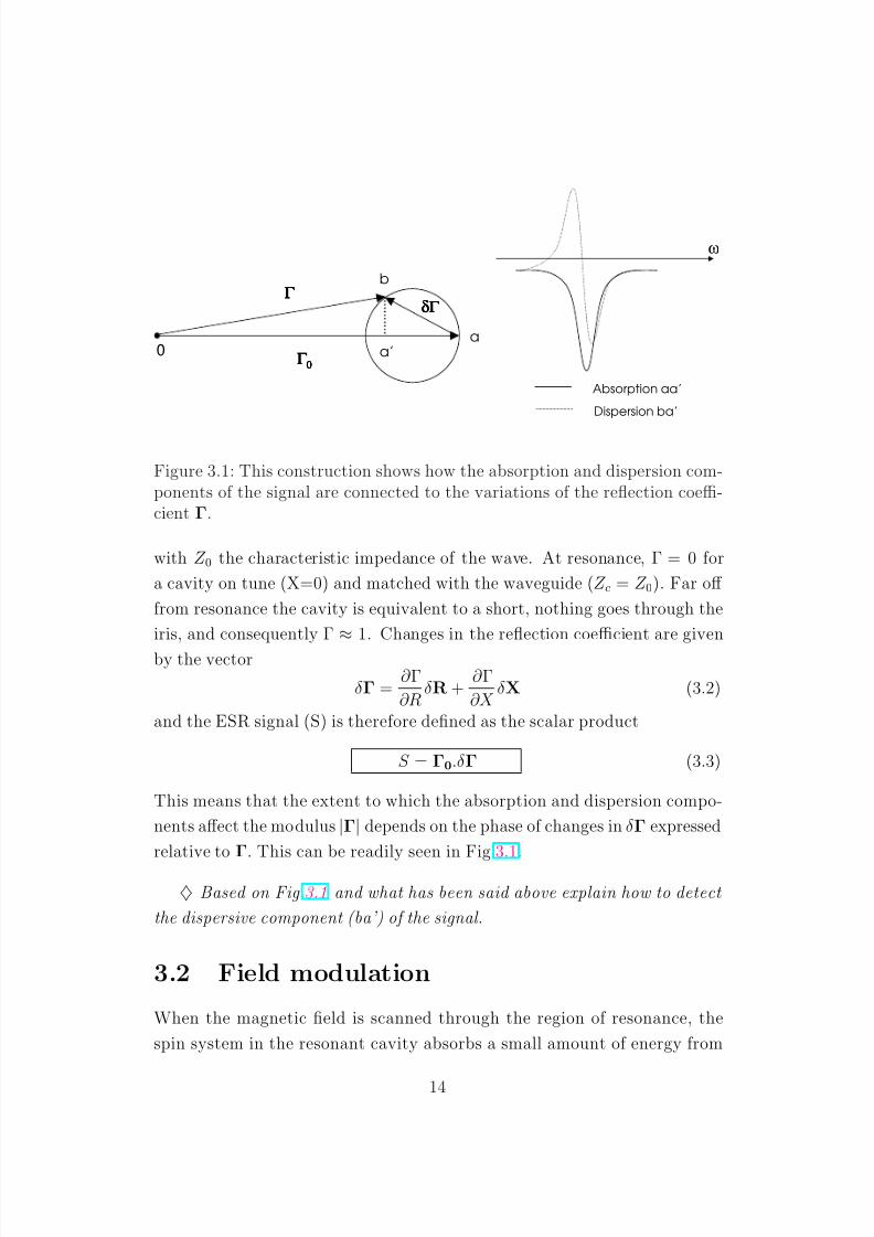
Figure 3.1: This construction shows how the absorption and dispersion com-ponents of the signal are connected to the variations of the reflection coeffi-cient Γ.
with Z 0 the characteristic impedance of the wave. At resonance, Γ = 0 for
a cavity on tune (X=0) and matched with the waveguide (Z c = Z 0). Far off
from resonance the cavity is equivalent to a short, nothing goes through the
iris, and consequently Γ ≈ 1. Changes in the reflection coefficient are given
by the vector
δΓ =∂ Γ
∂RδR +
∂ Γ
∂X δX (3.2)
and the ESR signal (S) is therefore defined as the scalar product
S = Γ0.δΓ (3.3)
This means that the extent to which the absorption and dispersion compo-
nents affect the modulus |Γ| depends on the phase of changes in δΓ expressed
relative to Γ. This can be readily seen in Fig.3.1.
♦ Based on Fig.3.1 and what has been said above explain how to detect
the dispersive component (ba’) of the signal.
3.2 Field modulation
When the magnetic field is scanned through the region of resonance, the
spin system in the resonant cavity absorbs a small amount of energy from
14
8/4/2019 Introduction to the Technique of Electron Spin Resonance (ESR) Spectroscopy
http://slidepdf.com/reader/full/introduction-to-the-technique-of-electron-spin-resonance-esr-spectroscopy 16/23
the microwave magnetic field H 1, and produces a slight change in the reso-
nant frequency of the microwave cavity. The DC detection of ESR is severely
limited, however, by the drift of the amplifier and the 1/f noise. For these rea-
sons, most ESR spectrometers incorporate magnetic field modulation which
transfers the relevant signal from DC to AC. The principle is the follow-
ing. When the magnetic field is modulated at the angular frequency ωm, an
alternating field1
2H m sinωmt (3.4)
superimposed on the constant magnetic field H 0 + H δ. H δ is the local field
induced by the surrounding of the considered electron. It is therefore H δ
which determines the broadening of the ESR line.
The ”constant” magnetic field is normally swept over the range ∆H 0 from
(H 0 −1
2∆H 0) to (H 0 + 1
2∆H 0) in a time t0 where H 0 is the magnetic field
strength at the center of the scan. At any time t during the scan, the instan-
taneous magnetic field strength H is given by
H = H 0 + H δ + H mod = H 0 + ∆H 0(t
t0−
1
2) +
1
2H m sinωmt (3.5)
where
H δ = ∆H 0(t
t0−
1
2) (3.6)
Consequently, the signal at the input of the detector is sinusoidal with the
frequency ωm and with an amplitude proportional to the derivative ∂s/∂H .
Note that in order to consider the field (H 0+H δ) as constant, the scan should
be slow enough so that there are many cycles of the modulation frequency
during the passage between the peak-to-peak (or half amplitude) points of
the resonance line.
♦ Sketch the effect of field modulation on the ESR line.
3.3 Principe of a phase-sensitive detection
A lock-in detector compares the ESR signal from the detector with a reference
signal and only passes the components of the former that have the proper
frequency and phase. If the reference voltage comes from the same oscillator
15

8/4/2019 Introduction to the Technique of Electron Spin Resonance (ESR) Spectroscopy
http://slidepdf.com/reader/full/introduction-to-the-technique-of-electron-spin-resonance-esr-spectroscopy 17/23
that produces the field modulation voltage, the ESR signal passes through
while noise is suppressed. Thus a lock-in detector only accepts signals that
”lock ” to the reference signal. Hence the name of ”phase-sensitive detector”.
The operation of a lock-in detector is simple. A reference oscillator produces
a reference signal vr
vr = V r cos(ωt + φ) (3.7)
where φ is a phase angle. At resonance the sample absorbs microwave energy
and produces the ESR signal voltage es
es = E s cos(ωt + φs) (3.8)
where φs is another phase angle that may be close to φ. The multiplier
produces an output that is the product esvr of the ESR signal and modulated
voltages
esvr = E sV r cos(ωt+φs)cos(ωt+φ) =1
2E sV r[cos(2ωt+φ+φs)+cos(φ−φs)]
(3.9)
The low pass filter removes the first term to produce the dc output voltage
V outV out =
1
2E sV r cos(φ− φs) (3.10)
and we see immediately that the sensitivity is maximal if φ is set equal to
φs, which gives
V out = 1
2E sV r (3.11)
When the electron spin resonance signal is measured by the lock-in am-
plifier it still contains a considerable amount of noise. A large part of this
noise may be removed by passing the signal through a low-pass filter. The
filter has associated with it a time constant or response time τ 0, which isa measure of the cutoff frequency of the filter. Another way to say this is
that the filter fails to pass frequencies that are much greater than the inverse
of the time constant 1/τ 0; it attenuates, distorts, and retards those incom-
ing waveforms that have frequencies in the vicinity of τ 0, and it transmits
undisturbed those frequencies considerably below 1/τ 0. The waveform that
is impressed on the ESR response filter may be considered as the derivative
of the absorption (or dispersion) line, and for comparison with the above
16
8/4/2019 Introduction to the Technique of Electron Spin Resonance (ESR) Spectroscopy
http://slidepdf.com/reader/full/introduction-to-the-technique-of-electron-spin-resonance-esr-spectroscopy 18/23
criteria, its effective frequency may be taken as the inverse of the time that
it takes to scan through the resonance from one peak to the next. In other
words, if the time that it takes to scan through the magnetic field range is
very short compared to the time constant τ 0, then no signal will appear on
the recorder; if this time equals the time constant, then a distorted signal
will result; while if one waits many time constants to complete the scan, then
the recorder will faithfully reproduce the true lineshape.
17
8/4/2019 Introduction to the Technique of Electron Spin Resonance (ESR) Spectroscopy
http://slidepdf.com/reader/full/introduction-to-the-technique-of-electron-spin-resonance-esr-spectroscopy 19/23
Chapter 4
Experiment
The following questions are of course suggestions and should not substitute
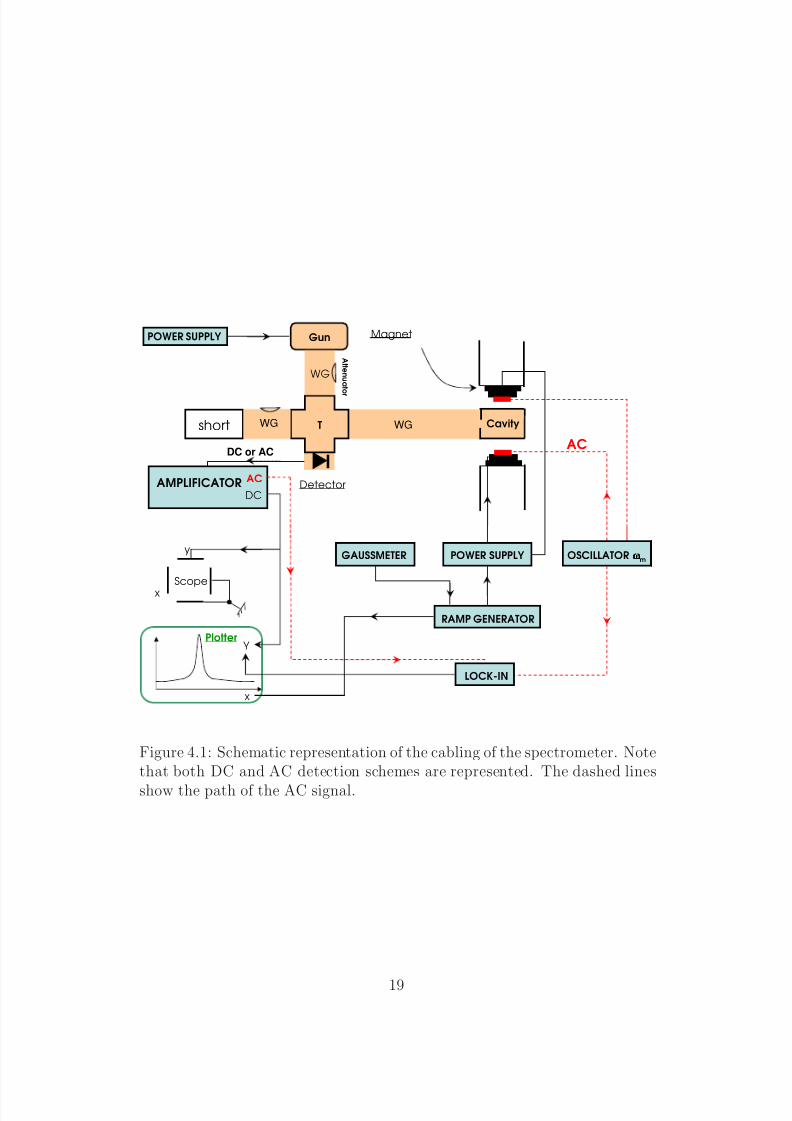
the initiative of the experimentalist. The cabling of the spectrometer is
described in Fig.4.1.
1. Read the manual and by doing so try to answer each of the exercises
marked with the symbol ♦
2. Measure the magnetic field as a function of the current in the magnet
for large and small, slow and fast field changes. Observe the hysteresis.
3. Measure the amplitude of the modulation of the field as a function of
the modulating current.
4. Measure the ESR signal on a powder sample of DPPH in absorption
and dispersion. Estimate the linewidth and the g-factor.
5. Measure the ESR signal of DPPH in solution for different concentration.
Estimate the dipole-dipole coupling constant. From that estimate the
range of concentration where the dipolar interaction becomes stronger
than the hyperfine interaction and compare with experiments.
6. Repeat 6 and 7 for Mn2+ in solution.
7. Observe and discuss the effect of varying the amplitude of the modu-
lating field on different ESR lines.
18
8/4/2019 Introduction to the Technique of Electron Spin Resonance (ESR) Spectroscopy
http://slidepdf.com/reader/full/introduction-to-the-technique-of-electron-spin-resonance-esr-spectroscopy 20/23
POWER SUPPLY
AC
DCAMPLIFICATOR
x
y
Scope
Y
x
Plotter
Gun
T
WG
At t en u at or
short WG
Detector
CavityWG
Magnet
GAUSSMETER POWER SUPPLY OSCILLATOR ωωωωm
RAMP GENERATOR
LOCK-IN
ACDC or AC
Figure 4.1: Schematic representation of the cabling of the spectrometer. Notethat both DC and AC detection schemes are represented. The dashed lines
show the path of the AC signal.
19
8/4/2019 Introduction to the Technique of Electron Spin Resonance (ESR) Spectroscopy
http://slidepdf.com/reader/full/introduction-to-the-technique-of-electron-spin-resonance-esr-spectroscopy 21/23
4.1 Bibliography
All the books listed below are in principle available at the library of the
physics department at ETH.
1. H. A. Atwater, Introduction to microwave theory , McGraw-Hill (1962)
2. C. P. Poole.Jr, Electron Spin Resonance, Interscience Publishers (1967)
3. A. Abragam and B. Bleaney, Electron Paramagnetic Resonance of Tran-
sition Ions, Clarendon Press . Oxford (1970)
4. D. J. E. Ingram, Radio and Microwave Spectroscopy , Butterworth &
Compagny (1976)
5. C. P. Poole.Jr. and H. A. Farach, Theory of Magnetic Resonance, 2nd
edition, Interscience Publishers (1987)
6. C. P. Slichter, Principle of Magnetic Resonance, 3rd edition, Springer
Verlag (1996)
20
8/4/2019 Introduction to the Technique of Electron Spin Resonance (ESR) Spectroscopy
http://slidepdf.com/reader/full/introduction-to-the-technique-of-electron-spin-resonance-esr-spectroscopy 22/23
Contents
1 Introduction 2
1.1 What is ESR? . . . . . . . . . . . . . . . . . . . . . . . . . . . 2
1.2 The hyperfine interaction . . . . . . . . . . . . . . . . . . . . . 4
1.3 The dipole-dipole interaction . . . . . . . . . . . . . . . . . . . 6
2 ESR spectrometer 7
2.1 Microwave parts . . . . . . . . . . . . . . . . . . . . . . . . . . 7
2.2 Electronic equipments . . . . . . . . . . . . . . . . . . . . . . 11
3 Detection scheme 13
3.1 ESR signal . . . . . . . . . . . . . . . . . . . . . . . . . . . . . 133.2 Field modulation . . . . . . . . . . . . . . . . . . . . . . . . . 14
3.3 Principe of a phase-sensitive detection . . . . . . . . . . . . . 15
4 Experiment 18
4.1 Bibliography . . . . . . . . . . . . . . . . . . . . . . . . . . . . 20
21
8/4/2019 Introduction to the Technique of Electron Spin Resonance (ESR) Spectroscopy
http://slidepdf.com/reader/full/introduction-to-the-technique-of-electron-spin-resonance-esr-spectroscopy 23/23
List of Figures
1.1 (a) Schematic representation of a single electron spin in a
steady magnetic field H0
(b) Corresponding energy-level scheme. 31.2 Splitting of the ESR line in Mn2+ owing to hyperfine interaction. 4
1.3 DDPH-Molecule(C6H5)2N − NC6H2(NO2)3 . . . . . . . . . . 5
2.1 ESR spectrometer . . . . . . . . . . . . . . . . . . . . . . . . . 8
2.2 Magic T. . . . . . . . . . . . . . . . . . . . . . . . . . . . . . . 9
2.3 The mode of the cavity used in our ESR spectrometer can
be monitored with a network-analyzer which measures the re-
flected power versus frequency. The vertical scale is logarith-
mic. The sharp dip shows the absorption of part of the incidentpower by the cavity. The amplitude of the dip quantifies the
amount of absorbed power by the cavity. Note that both the
amplitude of the dip and the frequency at which the mode
occurs change when a sample is introduced in the cavity. . . . 10
3.1 This construction shows how the absorption and dispersion
components of the signal are connected to the variations of
the reflection coefficient Γ. . . . . . . . . . . . . . . . . . . . 14
4.1 Schematic representation of the cabling of the spectrometer.
Note that both DC and AC detection schemes are represented.
The dashed lines show the path of the AC signal. . . . . . . . 19
22

![Multifrequency electron spin resonance in strongly ...real.mtak.hu/2533/1/60984_ZJ1.pdf · [Jánossy 2007] on the multifrequency ESR, magnetoresistance and magnetic field dependent](https://static.documents.pub/doc/80x56/5e3903cdea36336a835787a5/multifrequency-electron-spin-resonance-in-strongly-realmtakhu2533160984zj1pdf.jpg)


