Introduction - user.math.uzh.chuser.math.uzh.ch/spinolo/notes.pdf · LAURA V. SPINOLO Abstract....

NOTES ON THE STUDY OF THE VISCOUS APPROXIMATION OF

HYPERBOLIC PROBLEMS VIA ODE ANALYSIS

LAURA V. SPINOLO

Abstract. These notes describe some applications of the analysis of ordinary differen-tial equations to the study of the viscous approximation of conservation laws in one spacedimension. The exposition mostly focuses on the analysis of invariant manifolds like thecenter manifold and the stable manifold. The last section addresses a more specific issueand describes a possible way of extending the notions of center and stable manifold to someclasses of singular ordinary differential equations arising in the study of the Navier-Stokesequation in one space variable.

1. Introduction

In recent years, techniques coming from the study of ordinary differential equations (ODEs)have been applied to the analysis of systems of conservation laws in one space dimension,

ut + f(u)x = 0 where u(t, x) ∈ RN and (t, x) ∈ [0,+∞[×R. (1.1)

In the previous expression, t and x denote the partial derivatives with respect to the variablest and x respectively and the flux f : R

N → RN is a function of class C2. In view of physical

considerations (see e.g. Dafermos [7]) it is of great interest considering the second orderapproximation

uεt + f(uε)x = ε

(

B(uε)uεx

)

x, (1.2)

where B is an N ×N “viscosity matrix” satisfying suitable conditions and ε is a parameter,ε → 0+. In particular, the Navier-Stokes equation in one space variable can be written inthe form (1.2) and by setting ε = 0 it formally reduces to the Euler equation. For the timebeing, we focus on the Cauchy problem obtained by coupling (1.2) with the initial datum

u(0, x) = u0(x). (1.3)

Establishing general results on the convergence of the family of functions uε satisfying (1.2), (1.3)is still a mayor open problem, but partial results have been achieved and ODE techniqueshave often played an important role: see again Dafermos [7] for a complete overview and a listof references. Let us just mention the work by Bianchini and Bressan [3], which establishedconvergence (under suitable assumptions) of the family of functions uε solving (1.2), (1.3) inthe case of the “artificial viscosity” B(uε) ≡ I (identity matrix). The proof in [3] employs aspecial decomposition of the gradient uε

x obtained by relying on ODE analysis.These notes aim at providing an informal overview on some of the ODE techniques that

are more frequently applied to the study of the limit ε → 0+ of (1.2). The exposition is1

2 LAURA V. SPINOLO

addressed to non-experts, so notions are usually first introduced in a simplified context andthen discussed in more general situations. Also, in most cases these notes only providean heuristic idea of the proof of the the results that are introduced, and refer to books orto original research papers for a more rigorous discussion. The discussion has, of course,no sake of completeness: in particular, to simplify the exposition very few references areprovided. For a more satisfactory bibliography, one can refer to the books by Dafermos [7]and by Serre [19] (conservation laws and their viscous approximation). An extremely richexposition of the analysis of invariant manifolds for ODEs is in the book by Katok andHasselblatt [14] (see also the book by Perko [17]).

To simplify the exposition, most of the following sections (all but the last one) focus onthe case of the “artificial viscosity” B(uε) ≡ I, so that (1.2) reduces to

uεt + f(uε)x = εuε

xx. (1.4)

However, many of the considerations extend to more general cases (sometimes the extensionis not straightforward, though). The details concerning this extension can be found in theoriginal research papers that are quoted in the following sections.

Also, most of the analysis described in the following sections apply to the study of thenon-conservative case

uεt + A(uε, εuε

x)uεx = εB(uε)uε

xx, (1.5)

where A is a suitable N × N matrices. Note that (1.2) can be written in the form (1.5) bysetting A(uε, εuε

x) = Df(uε) − εB(uε)x, where Df denotes the Jacobian matrix of the fluxf . Again, the details concerning this extension are available in the original research papersquoted in the following sections.

The exposition is organized as follows: Section 2 informally describes the connectionbetween the analysis of the limit ε → 0+ of the viscous approximation (1.2) and the studyof ODEs by introducing the notions of traveling waves and boundary layers. Section 3deals with the Center Manifold Theorem and Section 4 mentions some applications to thestudy of the viscous approximation. Section 5 deals with the Stable Manifold Theorem,while the last section of these notes (Section 6) is more technical and describes a possibleway of extending the definition of center and stable manifold to a class of singular ordinarydifferential equations arising in the study of the viscous approximation defined by the Navier-Stokes equation in one space variable.

Acknowledgments. These notes were originally prepared for a course given at the SeventhMeeting on Hyperbolic Conservation Laws and Fluid Dynamics: Recent Results and ResearchPerspectives. The conference was held at SISSA, Trieste and was organized by Fabio Ancona,Stefano Bianchini, Rinaldo M. Colombo and Andrea Marson. The author warmly thank themfor the kind invitation.

VISCOUS APPROXIMATION VIA ODE ANALYSIS 3

2. Some motivations

This section aims at discussing some links between the study of the viscous approximationof a system of conservation laws in one space dimension and the ODE analysis by informallyillustrating the notions of traveling waves and boundary layers.

2.1. Traveling waves. Let us start with some heuristic considerations. For every ε > 0,(1.4) is a parabolic equation and one expects a strong regularizing effect. Conversely, itknown that, even if the initial datum u0 is smooth, nevertheless in general a classical solution(i.e., a solution of class C1) of the Cauchy problem (1.1), (1.3) may break down in finite time:remarkably, this may happen even in the scalar case N = 1 (see e.g. Dafermos [7, Chapter4.2]). Hence, when studying the limit ε→ 0+ one handles a family of very regular functionswhich is expected to converge to something which has a much weaker regularity. Travelingwaves are often regarded as useful tools to handle this behavior and to describe the formationof singularities in the limit.

To fix the notations, let us introduce the following definition.

Definition 2.1. Let u+, u− ∈ RN and σ ∈ R be given. The function U : R → R

N is atraveling wave for (1.2) joining the states u+, u− ∈ R

N and having speed σ if U(y) satisfies

U ′′ =[

f(U) − σU]′

(2.1)

andlim

y→−∞= u− lim

y→+∞= u+ (2.2)

In the previous expression, U ′ and U ′′ denote respectively the first and the second deriv-ative of U with respect to the variable y. Some observations are here in order. First, thelink between (2.1) and (1.4) is the following: if U solves (2.1), then one can verify by directcheck that a solution of (1.4) is obtained by setting

uε(t, x) := U

(

x− σt

ε

)

. (2.3)

Also, the function U is a solution of the ordinary differential equation (2.1), hence it is ofclass C2 and the same regularity is inherited by uε. However, by taking the pointwise limitε→ 0+ of uε we get

u(t, x) := limε→0+

uε(t, x) = limε→0+

U

(

x− σt

ε

)

=

limy→−∞ U(y) if x− σt < 0

limy→+∞ U(y) if x− σt > 0

One can then verify that the pointwise limit u(t, x) provides a distributional solution of (1.1).Summing up, we have that, if conditions (2.2) hold, then the solution of the parabolic

equation defined by (2.3) is regular for every ε > 0, but converges pointwise to a discontinuousdistributional solution of the conservation law. This is why traveling waves are often usedto study the non trivial behavior mentioned above, namely the appearance of singularitieswhen passing from the vanishing viscosity approximation to the hyperbolic limit.

4 LAURA V. SPINOLO

Let us now why the ODE analysis comes into play: the following considerations are quiteinformal, for a more precise and rigorous exposition see for example Bianchini and Bressan [3,Sections 3, 4]. Let us consider the equation (2.1): usually, the values u+, u− and σ are notprescribed. Conversely, one wants to understand for which values of u+, u− and σ there isa solution of (2.1) satisfying

limy→−∞

= u− limy→+∞

= u+.

To select a unique solution of (2.1), one needs to assign 2N+1 parameters: for example, onecan assign a Cauchy datum for U and for U ′ and the value of σ (remember that U takes valuesin R

N ). As a matter of fact, in many situations one does not manage to assign so manyconditions and apparently one ends up with an underdetermined problem. By assigning2N + 1 parameters, however, one is neglecting an important information: the values of u+

and u− are not prescribed, but nevertheless both the limits limx→± U(y) exist and are finite.In particular, this implies that U is bounded on the whole R. In many situations, oneactually has even more information: given a value u ∈ R

N , one looks for values of u+, u−

and σ satisfying the following property.

Both u+ and u− are close to u, σ is close to λi(u). (2.4)

Here λi(u) denotes the i-th eigenvalue of the Jacobian matrix Df(u). As we see in Section 3,the Center Manifold Theorem allows to exploit the information (2.4) to reduce the numberof conditions one needs to impose on (2.1) to select a unique solution.

2.2. Boundary layers. Boundary layer phenomena are observed when studying the viscousapproximation of initial boundary value problems.

To illustrate the heart of the matter, let us focus on a specific situation. Consider thefamily of problems

{


xx

uε(t, 0) = ub(t) uε(0, x) = u0(x).

As established in Ancona and Bianchini [1], under suitable assumptions on the data ub andu0, for every t ≥ 0 the family uε(t, ·) converges in L1

loc to u(t, ·), a distributional solutionof (1.1) satisfying the following condition: for every t ≥ 0, TotVarxu(t, ·) < +∞. The pointwhere boundary layers come into play is the fact that, in general, the boundary condition islost, namely (note that the limit below exists since the total variation is bounded)

limx→0+

u(t, x) 6= ub(t). (2.5)

See also the previous work by Gisclon [10] for the proof of the local in time convergence formore general viscous approximations (1.2).

To study the “loss” of boundary condition (2.5), the key point is the analysis of the steadysolutions of (1.4), satisfying f(u)x = εuxx. To understand why steady solutions are able tocapture this behavior (the loss of boundary condition), let us start by considering a toymodel.


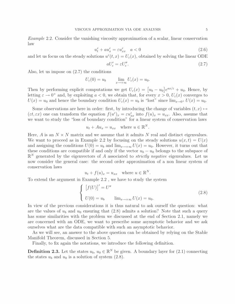
Example 2.2. Consider the vanishing viscosity approximation of a scalar, linear conservationlaw

uεt + auε

x = εuεxx a < 0 (2.6)

and let us focus on the steady solutions uε(t, x) = Uε(x), obtained by solving the linear ODE

aU ′ε = εU ′′

ε . (2.7)

Also, let us impose on (2.7) the conditions

Uε(0) = ub limx→+∞

Uε(x) = u0.

Then by performing explicit computations we get Uε(x) =[

ub − u0

]

eax/ε + u0. Hence, byletting ε → 0+ and, by exploiting a < 0, we obtain that, for every x > 0, Uε(x) converges toU(x) = u0 and hence the boundary condition Uε(x) = ub is “lost” since limx→0+ U(x) = u0.

Some observations are here in order: first, by introducing the change of variables (t, x) 7→(εt, εx) one can transform the equation f(uε)x = εuε

xx into f(u)x = uxx. Also, assume thatwe want to study the “loss of boundary condition” for a linear system of conservation laws

ut + Aux = uxx where u ∈ RN .

Here, A is an N ×N matrix and we assume that it admits N real and distinct eigenvalues.We want to proceed as in Example 2.2 by focusing on the steady solutions u(x, t) = U(x)and assigning the conditions U(0) = ub and limx→+∞ U(x) = u0. However, it turns out thatthese conditions are compatible if and only if the vector ub − u0 belongs to the subspace ofR

N generated by the eigenvectors of A associated to strictly negative eigenvalues. Let usnow consider the general case: the second order approximation of a non linear system ofconservation laws

ut + f(u)x = uxx where u ∈ RN .

To extend the argument in Example 2.2 , we have to study the system

[

f(U)]′

= U ′′

U(0) = ub limx→+∞ U(x) = u0.(2.8)

In view of the previous considerations it is thus natural to ask ourself the question: whatare the values of ub and u0 ensuring that (2.8) admits a solution? Note that such a queryhas some similarities with the problem we discussed at the end of Section 2.1, namely weare concerned with an ODE, we want to prescribe some asymptotic behavior and we askourselves what are the data compatible with such an asymptotic behavior.

As we will see, an answer to the above question can be obtained by relying on the StableManifold Theorem, discussed in Section 5.

Finally, to fix again the notations, we introduce the following definition.

Definition 2.3. Let the states ub, u0 ∈ RN be given. A boundary layer for (2.1) connecting

the states ub and u0 is a solution of system (2.8).

6 LAURA V. SPINOLO

3. The Center manifold Theorem

In this section we are concerned with studying the asymptotic behavior of the solutionsof the ordinary differential equation

V ′ = G(V ) where V ∈ Rd

in a neighborhood of an equilibrium point V . Without any loss of generality we can assumeV = ~0, namely G(~0) = ~0. In Section 4 we will then apply our analysis to the study of thesystem (2.1).

Let us start by considering two simple examples where G is linear.

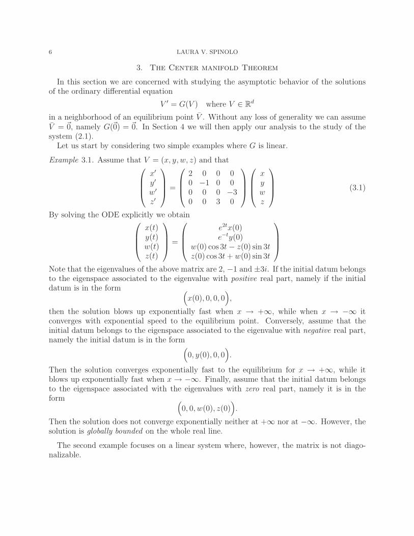
Example 3.1. Assume that V = (x, y, w, z) and that

x′

y′

w′

z′

=

2 0 0 00 −1 0 00 0 0 −30 0 3 0

xywz

(3.1)

By solving the ODE explicitly we obtain

x(t)y(t)w(t)z(t)

=

e2tx(0)e−ty(0)

w(0) cos 3t− z(0) sin 3tz(0) cos 3t+ w(0) sin 3t

Note that the eigenvalues of the above matrix are 2, −1 and ±3i. If the initial datum belongsto the eigenspace associated to the eigenvalue with positive real part, namely if the initialdatum is in the form

(

x(0), 0, 0, 0)

,

then the solution blows up exponentially fast when x → +∞, while when x → −∞ itconverges with exponential speed to the equilibrium point. Conversely, assume that theinitial datum belongs to the eigenspace associated to the eigenvalue with negative real part,namely the initial datum is in the form

(

0, y(0), 0, 0)

.

Then the solution converges exponentially fast to the equilibrium for x → +∞, while itblows up exponentially fast when x → −∞. Finally, assume that the initial datum belongsto the eigenspace associated with the eigenvalues with zero real part, namely it is in theform

(

0, 0, w(0), z(0))

.

Then the solution does not converge exponentially neither at +∞ nor at −∞. However, thesolution is globally bounded on the whole real line.

The second example focuses on a linear system where, however, the matrix is not diago-nalizable.


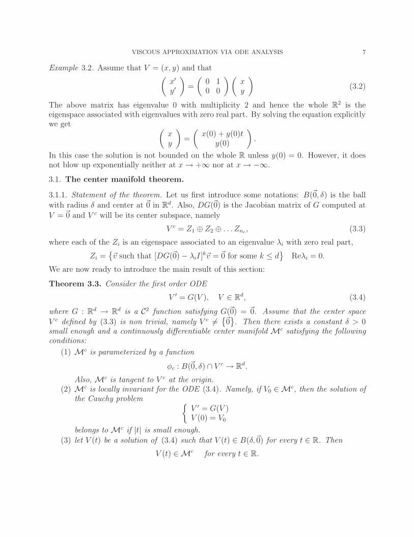
Example 3.2. Assume that V = (x, y) and that(

x′

y′

)

=

(

0 10 0

) (

xy

)

(3.2)

The above matrix has eigenvalue 0 with multiplicity 2 and hence the whole R2 is the

eigenspace associated with eigenvalues with zero real part. By solving the equation explicitlywe get

(

xy

)

=

(

x(0) + y(0)ty(0)

)

.

In this case the solution is not bounded on the whole R unless y(0) = 0. However, it doesnot blow up exponentially neither at x→ +∞ nor at x→ −∞.

3.1. The center manifold theorem.

3.1.1. Statement of the theorem. Let us first introduce some notations: B(~0, δ) is the ball

with radius δ and center at ~0 in Rd. Also, DG(~0) is the Jacobian matrix of G computed at

V = ~0 and V c will be its center subspace, namely

V c = Z1 ⊕ Z2 ⊕ . . . Znc, (3.3)

where each of the Zi is an eigenspace associated to an eigenvalue λi with zero real part,

Zi ={

~v such that [DG(~0) − λiI]k~v = ~0 for some k ≤ d

}

Reλi = 0.

We are now ready to introduce the main result of this section:

Theorem 3.3. Consider the first order ODE

V ′ = G(V ), V ∈ Rd, (3.4)

where G : Rd → R

d is a C2 function satisfying G(~0) = ~0. Assume that the center space

V c defined by (3.3) is non trivial, namely V c 6={

~0}

. Then there exists a constant δ > 0small enough and a continuously differentiable center manifold Mc satisfying the followingconditions:

(1) Mc is parameterized by a function

φc : B(~0, δ) ∩ V c → Rd.

Also, Mc is tangent to V c at the origin.(2) Mc is locally invariant for the ODE (3.4). Namely, if V0 ∈ Mc, then the solution of

the Cauchy problem{

V ′ = G(V )V (0) = V0

belongs to Mc if |t| is small enough.

(3) let V (t) be a solution of (3.4) such that V (t) ∈ B(δ,~0) for every t ∈ R. Then

V (t) ∈ Mc for every t ∈ R.

8 LAURA V. SPINOLO

An important remark is that the center manifold (3.4) about the equilibrium point ~0 is notunique (see for example the lecture notes by Bressan [6] for an explicit example). In otherwords, suitable examples show that in general there is more than one manifold satisfyingconditions (1)..(4) in the statement of the theorem. We will come back to this point in theproof of the theorem, when it will be clear where this lack of uniqueness come from.

The proof of Theorem 3.3 discussed in here is the same as in the notes by Bressan [6]. Fora more general viewpoint, one can refer to the book by Katok and Hasselblatt [14].

3.2. Proof of Theorem 3.3. The proof is divided in several steps, and only some of themare provided below (see [6] for the complete argument).Step 1: heuristic. The heuristic idea is that the manifold Mc should play the role thatin the linear case is played by the center space. In exploiting this idea one should keep inmind that, as Example 3.2 shows, the solutions of a linear system lying on the center spacein general are not bounded on the whole real line: the only requirement we can reasonablyimpose is that they did not blow up exponentially fast neither at +∞ nor at −∞.

To make an extension to the general non linear case we have to handle some technicaldifficulties. First of all, we need to introduce a localization argument. Also, because of thenon linearity we cannot require that the solutions lying on the center manifold do not blowexponentially neither at +∞ nor at −∞, but only that they are controlled by exp(η|t|),where η is a small positive constant.Introduction of a cut-off function Let

p(V ) = G(V ) −DG(0)V

be the second order term in the expansion of G. We then have

|p(V )| ≤ C|V |2 and |Dp(V )| ≤ CV (3.5)

for a suitable constant C and for V in a small enough neighborhood of ~0.We want to reduce to the case p has compact support and small C1 norm. We thus

introduce a smooth, even cut-off function ρ : R → R satisfying

0 ≤ ρ(t) ≤ 1 for every t ∈ R and ρ(t) =

{

1 if |t| ≤ 10 if |t| ≥ 2

We then define

pδ(V ) := p(V ) ρ(|V |/δ),thus obtaining that the support of pδ is contained in B(~0, 2δ). In the previous expression,δ denotes a small constant whose exact value is determined in the following. By relyingon (3.5) we also get

‖pδ‖C0 ≤ supX∈B(~0,2δ)

|p(V )| ≤ 4Cδ2

and

|Dpδ(V )| = |Dp(V )|ρ+ |p(V )| |ρ′| 1

δ≤ Cδ.


By combing the previous observations we can make the C1 norm arbitrarily small by choosingδ small enough.

In the following, we will study the solutions of the ODE

V ′ = DG(0)V + pδ(V ). (3.6)

By construction,

DG(0)V + pδ(V ) = G(V ) when |V | ≤ δ

and hence any claim holding for the solutions of (3.6) holds for the solutions of the original

equation V ′ = G(V ) confined in B(~0, δ).Step 3: definition of a fixed point problem We first have to introduce some furthernotations: for simplicity, in the following we denote by A the Jacobian matrix DG(~0). Also,the stable and unstable space of A are the subspaces of R

d associated to the eigenvalues withnegative and positive real part respectively. Namely,

V s = N1 ⊕N2 ⊕ . . . NnsV u = P1 ⊕ P2 ⊕ . . . Pnu

(3.7)

where the Ni and the Pi are eigenspaces associated with eigenvalues with negative andpositive real part respectively:

Ni ={

~v ∈ Rd :

(

A− λiI)kv = ~0 for some k ≤ d} Reλi < 0

and

Pi ={

~v ∈ Rd :

(

A− λiI)kv = ~0 for some k ≤ d} Reλi > 0.

In particular, since

Rd = V s ⊕ V u ⊕ V c,

then any x ∈ Rd satisfies x = πsx+ πux+ πcx, where

πs : Rd → V s πu : R

d → V u πc : Rd → V c

are the projections onto V s, V u and V c respectively.Note that the ODE

V ′ = AV + pδ(V )

can be then written as the coupling of the ODEs

(

πsV)′

= AπsV + πspδ(V )

(

πuV)′

= AπuV + πupδ(V )

(

πcV)′

= AπcV + πcpδ(V ).

We have exploited the following equalities:

πsAV = AπsV πuAV = AπuV πcAV = AπcV for every V ∈ Rd

10 LAURA V. SPINOLO

We solve each equation separately and by applying the “variation of constants” formula weobtain that the components πsV (t), πuV (t) and πcV (t) satisfy

πsV (t) = eA(t−ts)πsV (ts) +

∫ t

ts

eA(t−s)πspδ(V (s))ds

πuV (t) = eA(t−tu)πuV (tu) +

∫ t

tu

eA(t−s)πupδ(V (s))ds

πcV (t) = eA(t−tc)πcV (tc) +

∫ t

tc

eA(t−s)πcpδ(V (s))ds.

(3.8)

In the previous expression, ts, tu and tc denote real values which will be assigned in thefollowing. Also, we have exploited the standard notation

exp(At) =∞

∑

n=0

tnAn

n!.

Let λi denote as before an eigenvalue of A, then we set

β+ := min{Reλi : Reλi > 0}and

β− := min{−Reλi : Reλi < 0}.There exists some constant C > 0 such that, for every ~v ∈ R

d, we have

|eAtπu~v| ≤ Ceβ+t/2|~v| for every t < 0 and |eAtπs~v| ≤ Ce−β−

t/2|~v| for every t > 0. (3.9)

We now fix a constant positive constant η > 0 satisfying

η < min

{

β+

2,β−2

}

and setYη :=

{

V ∈ C0(] −∞,+∞[; Rd}

such that supt∈R

|V (t)|e−η|t| < +∞}

.

Then Yη equipped with the norm

‖V ‖η := supt∈R

|V (t)|e−η|t|

is a Banach space. Note that

|V (t)| ≤ eη|t|‖V ‖η for every t ∈ R, V ∈ Yη.

Loosely speaking, the space Yη contains all the function which “do not blow up with too fastexponential speed” neither at +∞ nor at −∞.

The goal is now defining the map φc by solving a suitable fixed point problem in Yη. First,we observe that, if the function V ∈ Yη, then by relying on (3.9) we get that, for any ts ≤ t,

|eA(t−ts)πsV (ts)| ≤ e−β−

(t−ts)/2e−ηts‖V ‖η = e−β−

t/2‖V ‖ηe(−η+β

−/2)ts


and hencelim

ts→−∞|eA(t−ts)πsV (ts)| = 0 for any given t ∈ R.

In the same way one can show that, if the function V ∈ Yη, then

limtu→+∞

|eA(t−tu)πuV (tu)| = 0 for any given t ∈ R.

We now go back to formula (3.8), we set tc = 0, xc = πcV (0) and we let ts → −∞ andtu → +∞, eventually obtaining

V (t) =πcV (t) + πsV (t) + πuV (t) = eAtxc +

∫ t

0

eA(t−s)πcpδ(V (s))ds

+

∫ t

−∞

eA(t−s)πspδ(V (s))ds+

∫ t

+∞

eA(t−s)πupδ(V (s))ds

(3.10)

for every V ∈ Yη.Further steps in the proof of the Center Manifold Theorem

• By applying the Contraction Map Theorem, one can show that, for any xc ∈ V c,the fixed point problem (3.10) admits a unique solution V ∈ Yη. To verify that thehypotheses of the Contraction Map Theorem are satisfied one has to exploit that pδ

is a function with compact support and small C1 norm.• The map

φc : V c → Rd

which parameterizes the center manifold is then defined by setting

φc(xc) := V (0). (3.11)

• One can then prove that such a map is continuously differentiable and that thetangent space at the origin is V c.

• By construction, the map φc satisfies the following properties: first, for any xc ∈ V c,the solution of the Cauchy problem

V ′ = AV + pδ(V )

V (0) = φc(xc)(3.12)

belongs to Yη, and hence it “does not blow up with fast exponential speed” neitherat +∞ nor at −∞. Conversely, any solution of (3.12) verifying

supt

|V (t)|e−η|t| < +∞

satisfies V (0) = φc(xc) for some xc ∈ V c.• We set Mc := φc(Vc) and we eventually come back to the original equation V ′ =G(V ). As pointed out before, G(V ) = DG(0)V +pδ(V ) when |V | < δ. Consequently,any claim concerning the solution of V ′ = DG(0)V + pδ(V ) can be reformulated in a

claim concerning the solutions of V ′ = G(V ) which are confined in B(~0, δ) for everyt ∈ R. By relying on this observation one concludes the proof of Theorem 3.3.

12 LAURA V. SPINOLO

A remark concerning non-uniqueness As pointed out before, in general the centermanifold of (3.4) about a given equilibrium point is not unique. The reason is that in theproof we have some freedom in choosing the cut-off function ρ: hence, both the map φc

defined as in (3.11) and the manifold Mc depend on the choice of ρ and are not unique.

4. Some applications of the Center Manifold Theorem to the analysis of

traveling waves

The Center Manifold Theorem has been applied by several authors to the analysis travel-ing waves: see Dafermos [7] for a list of references. In this section we will discuss a possibleapproach, due to Bianchini and Bressan [3] and in the second part we will deal with appli-cations to the study of the vanishing viscosity approximation uε

t + f(uε)x = εuεxx.

4.1. A center manifold of traveling waves. Let us now go back to the problem wediscussed at the end of Section 2.1: we are given the traveling wave equation

U ′′ =[

f(U) − σU]′

where U ∈ RN (4.1)

and a value u ∈ RN . We want find solutions U admitting finite limits both at x → ±∞,

limy→±∞ = u± and satisfying the following properties: first, for every y ∈ R, U(y) belongsto a small neighborhood of u. Also, σ is close to λi(u), where λi(u) is a given eigenvalue ofthe Jacobian matrix Df(u). More precisely, we want to exploit the information we have onU to reduce the number of conditions one has to assign on (4.1) to select a unique solution.

By setting p := U ′ we get that (4.1) can be written as the first order system

U ′ = pp′ =

[

Df(U) − σI]

pσ′ = 0.

(4.2)

We now apply the Center Manifold Theorem: first, we observe that the point V =(

U ,~0, λi(U))

is an equilibrium for (4.2). Hence, from the third claim in the statement of Theorem 3.3 wededuce the following. There exists a constant δ > 0 and a center manifold Mc such thatany solution of (4.2) satisfying

|(

U(y), p(y), σ)

− V | ≤ δ for every y ∈ R (4.3)

lies on Mc. As we mentioned in Section 3, the center manifold of a system about a givenequilibrium point is in general non-unique. In the following we will arbitrarily fix one centermanifold and denote it by Mc.

We now want to investigate the structure of Mc. First, we compute its dimension, whichis the dimension of the center space. By setting

V =(

U, p, σ)t

and G(V ) =(

p,[

Df(U) − σI]

p, 0)t


we get that V ∈ R2N+1 and the Jacobian matrix DG(V ) is given by

DG(V ) =

0 I ~0

0 Df(u) − λi(u)I ~00 0 0

. (4.4)

In the previous expression, 0 and I denote the null and the identityN×N matrix respectively.Let us assume that the matrix Df(u) has N real and distinct eigenvalues: this hypothesisof so-called strict hyperbolicity is quite standard in the study of conservation laws (see forexample Dafermos [7, Section 9.6] for a discussion on the “bad behaviors” exhibited bysystems violating strict hyperbolicity). Let ~ri denote a unit eigenvector associated to λi(u),namely

[

Df(u) − λi(u)]

~ri = ~0 and |~ri| = 1.

Then the center space of the matrix (4.4) is

V c ={

(u, p, σ) such that u ∈ RN , p = a~ri for some a ∈ R, and σ ∈ R

}

.

Hence, the dimension of V c and of Mc is N+2. This gives an answer to one of the questionswe asked ourselves: if we are looking for solutions of (4.2) satisfying (4.3), we need to imposeN + 2 conditions (instead of 2N + 1) to select a unique solution.

Let us get some more precise information about the structure of Mc. Let

φc : B(~0, δ) ∩ V c → R2N+1 (4.5)

be a parameterization of Mc. From the proof of Theorem 3.3 we infer that φc can be chosenin such a way that πc◦φc(xc) = xc for any xc ∈ V c. By applying this property to system (4.2)we get

πc ◦ φc(U, a~ri, σ) = (U, a~ri, σ) for every U ∈ RN , a ∈ R, σ ∈ R. (4.6)

and hence

φc(U, a~ri, σ) =(

U, ψc(U, a, σ), σ)

,

where ψc : V c → RN is a suitable function whose properties we want to investigate. Let

{~r1 . . . ~rN} be a basis of RN entirely made by unit eigenvectors of Df(u). Then we denote

by ψ1c . . . ψNc the corresponding components of ψc and we get

ψc(U, a, σ) =N

∑

k=1

ψkc(U, a, σ)~rk. (4.7)

To write (4.7) in a more convenient form, we first exploit (4.6) to get ψic(U, a, σ) = a. Also,

any point (U,~0, σ) is an equilibrium for (4.2), so it belongs to Mc. This implies that

~0 =

N∑

k=1

ψkc(U, a, σ)~rk and hence that ψkc(U, 0, σ) = 0 for every k, U and σ.

14 LAURA V. SPINOLO

By exploiting the regularity of the map ψkc, we deduce that ψkc(U, a, σ) = aψkc(U, a, σ) for

a suitable function ψkc. By combining the previous observations we then get that (4.7) canbe rewritten as

p = a(

~ri +∑

k 6=i

ψkc(U, a, σ)~rk

)

.

Since Mc is tangent at the equilibrium point to the center space V c we also have(

~ri +∑

k 6=i

ψkc(U , 0, λi(U))~rk

)

= ~ri, (4.8)

namely ψkc(U , 0, λi(U)) = 0 for every k 6= i. By setting

ri(U, a, σ) :=(

~ri +∑

k 6=i

ψkc(U, a, σ)~rk

)

,

we then obtain that (4.7) can be rewritten as

p = ari(U, a, σ).

For convenience, we want to reduce to the case of unit vectors, so we write the above relationas

p = a|ri(U, a, σ)| ri(U, a, σ)

|ri(U, a, σ)| ,

where |ri(U, a, σ)| denotes the length of the vector. Note that (4.8) implies that ri(U , 0, λi(U)) =~ri. Hence, the map

a 7→ v(a) = a|ri(U, a, σ)|is locally invertible in a neighborhood of (U , 0, λi(U)): by assuming that the size of theconstant δ in (4.5) is small enough, we eventually get that the manifold Mc is described bythe relation

p = vri(U, v, σ), (4.9)

where we have set ri = ri/|ri|.4.2. Center manifold and convergence of the vanishing viscosity approximation.

In this section we just mention the fact that center manifold techniques have been exploitedby Bianchini and Bressan [3] to show the convergence of the solutions of the family of Cauchyproblems

{


xx

uε(0, x) = u0(x).(4.10)

More precisely, the following holds.

Theorem 4.1 (Theorem 1 page 229 in [3]). Assume that the flux function f : RN → R

N isof class C2 and that, for every u ∈ R

N , the jacobian matrix Df(u) has N real and distincteigenvalues. There exists a small enough constant δ > 0 such that, if the initial datumin (4.10) satisfies

u0 ∈ L1(R) and TotVar{u0} ≤ δ,


then the following properties hold.

(1) For any ε > 0, the Cauchy problem (4.10) admits a solution defined for any t ≥ 0.Also, there exists a constant C, which does not depend neither on ε nor on t, suchthat

TotVarx{uε(t, ·)} ≤ Cδ. (4.11)

(2) The solution uε is stable in L1 with respect to time and to L1 perturbation of theinitial data. Namely, if by using a semigroup notation we denote by t 7→ Sε

tu0 thesolution of (4.10), then

‖Sεt u0 − Sε

sv0‖L1 ≤ L(

‖u0 − v0‖L1 + |t− s| + |√εt−

√εs|

)

for every t, s ≥ 0.

In the previous expression, L denotes a constant which does not depend neither on εnor on the time.

(3) As ε → 0+, for every t ≥ 0, Sεt u0 converges strongly in L1

loc(R) to a function Stu0

providing a distributional solution of (4.10). Also, the semigroup t 7→ Stu0 enjoysthe stability property

‖Stu0 − Ssv0‖L1 ≤ L(

‖u0 − v0‖L1 + |t− s|)

for every t, s ≥ 0.

4.3. Solutions of the Riemann problem. In this section, as a direct application of thecenter manifold construction discussed in Section 4.1, we go over the analysis of the solutionof the so-called Riemann problem

ut + f(u)x = 0

u(0, x) =

{

u+ x > 0u− x < 0

(4.12)

Here u+ and u− are two given values in RN and in the following we focus on the case

|u+−u−| < δ for a small enough constant δ. The Riemann problem is a very specific exampleof Cauchy problem, but is nonetheless extremely important. Indeed, its study provides thebuilding block for the construction of approximation schemes (Glimm scheme [11], wavefront-tracking algorithm) that have been used to establish global existence and uniquenessresults for the system of conservation laws ut + f(u)x = 0: see for example Dafermos [7,Chapter 14] and the references therein.

The first issue one has to address when studying (4.12) is that, in general, a distribu-tional solution of (4.12) is not unique: in the attempt to select a unique solution, variousadmissibility criteria have been introduced. An admissibility criterium was introduced byLax [15], who also constructed an admissible solution of (4.12). The analysis in [15] reliedon some technical assumptions on the flux f which were later relaxed in Liu [16]. See alsoTzavaras [20] and Joseph and LeFloch [13]. Bianchini and Bressan [3, Section 14] provideda general construction of an admissible solution obtained by taking the limit ε → 0+ of the

16 LAURA V. SPINOLO

vanishing viscosity approximation


xx

uε(0, x) =

{

u+ x > 0u− x < 0

In both [15, 16] and [3] the key point is the construction of the so-called i-wave fan curve.Loosely speaking, the basic idea is the following: given u− ∈ R

N , the i-wave fan curveTi(u

−, s) contains all the states u+ such that an admissible solution of the Riemann prob-lem (4.12) is obtained by gluing shocks (or contact discontinuities) and rarefaction wavesbelonging to the i-family. In particular, this implies that there is a self-similar, admissiblesolution u(t, x) = U(x/t) of (4.12) such that U(ξ) varies only in a small neighborhood of theeigenvalue λi(u

−) and is constant elsewhere, U(ξ) = u− for ξ < λi(u−) − δ and U(ξ) = u+

for ξ > λi(u−) + δ.

We now informally go over the main steps of the construction in [3].

(1) We fix u− ∈ RN and we consider the same ri as in (4.9), obtained by applying the

Center Manifold Theorem to system (4.2) about the equilibrium point(

u−,~0, λi(u−)

)

.Here λi(u

−) is the i-eigenvalue of Df(u−). Given s > 0, we consider the followingfixed point problem, defined on the interval [0, s]:

u(τ) = u− +

∫ τ

0

ri(u(ξ), vi(ξ), σi(ξ))dξ

vi(τ) = fi(τ, u, vi, σi) − convfi(τ)

σi(τ) =d

dτconvfi(τ).

(4.13)

Here

fi(τ) =

∫ τ

0

λi(u(ξ), vi(ξ), σi(ξ))dξ and λi(u(ξ), vi(ξ), σi(ξ)) = 〈A(u)ri, ri〉,

namely λi can be regarded as a generalized eigenvalue. Also, convfi(τ) denotes theconvex envelope of fi(τ),

convfi(τ) = sup{

g(τ) s.t. g is convex, g(ξ) ≤ f(ξ) for every ξ ∈ [0, s]}

.

By relying on the Contraction Map Theorem, one can show that (4.13) admits aunique continuous solution

(

u(τ), vi(τ), σi(τ))

defined in a small enough neighbor-

hood of (u−, 0, λi(u−). The functions

(


are all defined on the interval[0, s].

(2) Assume that the interval [a, b] ⊆ [0, s] satisfies the following property: for everyτ ∈ [a, b], fi(τ) = convfi(τ). Then one can show that ri

(


= ri

(

u(τ))

for every τ ∈ [a, b] and moreover that the solution of the Riemann problem

ut + f(u)x = 0

u(0, x) =

{

u(b) x > 0u(a) x < 0


is a rarefaction wave of the i-th family (hence, in particular, the solution is continu-ously differentiable in ]0,+∞[×R).

(3) Conversely, assume that for every τ ∈]c, d[⊆ [0, s], fi(τ) > convfi(τ) and that fi(c) =convfi(c), fi(d) = convfi(d). Then, in particular, one can show that σi is constanton [c, d], σi = σi. Also, vi(τ) > 0 on ]c, d[ and one can define the change of variables

dx

dt=

1

vi(t)

x(0) =d− c

2

mapping x : ]c, d[→] −∞,+∞[. Let τ(x) denote its inverse: one can show that thefunction U(x) := u

(

τ(x))

satisfies

U ′′ =(

f(U) − σiU)′

and limx→−∞

U(x) = u(c), limx→+∞

U(x) = u(d).

In other words, there is a traveling wave connecting u(c) and u(d) and hence a solutionof the Riemann problem

ut + f(u)x = 0

u(0, x) =

{

u(d) x > 0u(c) x < 0

is

u(t, x) =

{

u(d) x > σitu(c) x < σit,

which is called either shock or contact discontinuity depending on the values ofλi

(

u(d))

and λi

(

u(c))

(see for example the book by Dafermos [7, Page 213] for theexact definition).

(4) By relying on the previous steps and on further approximation arguments, one canshow that if

(


is the solution of (4.13), then the family uε solving


xx

uε(0, x) =

{

u− x < 0u(s) x > 0

converges ε → 0+ to the function

u(t, x) =

u− if x < σi(0)tu(τ) if x = σi(τ)tu(s) if x > σi(s)t

We then define the i-wave fan curve by setting Ti(u−, s) := u(s).

(5) When s < 0, the construction of Ti(u−, s) is analogous, the only difference being that

in (4.13) one has to take the concave envelope of fi instead of the convex one.

18 LAURA V. SPINOLO

Finally, observe that the above construction can be extended to study the solution of theRiemann problem (4.12) obtained by taking the limit ε → 0+ of the more general viscousapproximation

uεt + f(uε)x = ε

(

B(uε)uεx

)

x,

under quite general assumptions on the matrix B (see Bianchini [2]). For extensions to theanalysis of initial-boundary value problems see Bianchini and Spinolo [5].

5. Stable Manifold Theorems

5.1. The Stable Manifold Theorem. Let us first recall some notations: given the ODE

V ′ = G(V ), (5.1)

let V be an equilibrium point, which without any loss of generality is assumed to be ~0. Asbefore, we denote by V s and V u the stable and the unstable space respectively, defined asin (3.7). Also, as usual, DG(~0) denotes the Jacobian matrix of G computed at ~0.

Theorem 5.1. Consider the first order ODE (5.1) where G : Rd → R

d is a C2 function

satisfying G(~0) = ~0. If V s is non trivial, namely V s 6= {~0}, then there exists a constant δ > 0small enough such there exists a continuously differentiable stable manifold Ms satisfying thefollowing conditions.

(1) Ms is parameterized by a function

φs : B(~0, δ) ∩ V s → Rd.

Also, Ms is tangent to V s at the origin.(2) Ms is locally invariant for the ODE (3.4). Namely, if V0 ∈ Ms, then the solution of

the Cauchy problem{

V ′ = G(V )V (0) = V0

(5.2)

satisfies V (t) ∈ Ms for every |t| small enough.(3) If V0 ∈ Ms then the solution of the Cauchy problem (5.2) satisfies

limt→+∞

|V (t)|ect/2 = 0, (5.3)

where

c = min{−Reλi such that λi is an eigenvalue of DG(~0), Reλi < 0} (5.4)

(4) Conversely, if V (t) is a solution of (5.1) satisfying (5.3), then V (t) ∈ Ms for everyt large enough.

The proof of Theorem 5.1 can be obtained by relying on an argument somehow similarto the one exploited in the proof of Theorem 3.3: a detailed proof can be found in thebook by Perko [17] (see also the book by Katok and Hasselblatt [14] for a more generalviewpoint). One should keep in mind, however, that the stable manifold (i.e., a manifoldsatisfying properties (1), (2), (3) and (4) in the statement of Theorem 5.1) is unique, while


the center manifold is not. As a matter of fact, one can also define a global stable manifoldas

Mgs =⋃

t≤0

{V (t) solving (5.1) and satisfying V (0) ∈ Ms}.

In this way, we obtain a manifold which is globally invariant for (5.1). Namely, if V0 ∈ Mgs,then the solution V (t) of (5.2) satisfies V (t) ∈ Mgs for every t.

5.2. Applications to the analysis of the boundary layers. Let us now go back to theoriginal problem described at the end of Section 2.2: given u0, we want to describe the valuesof ub such that problem

{

U ′ = f(U) − f(u0)U(0) = ub limx→+∞U(x) = u0

admits a solution. By combining parts (2) and (3) in the statement of the theorem we getthat the previous problem admits a solution provided ub belongs to the stable manifold Ms,whose dimension is equal to the number of the eigenvalues of Df(u0) with negative real part.If all the eigenvalues of the Jacobian matrix Df(u0) have nonzero real part, then as a matterof fact one can also prove the converse implication: if the above problem admits a solution,then ub ∈ Ms.

5.3. The slaving manifold of a manifold of equilibria. Loosely speaking, the StableManifold Theorem we discussed in the previous section describes all the solutions of (5.1)

that when t→ +∞ converge exponentially fast to the equilibrium point ~0.Let us consider a more general situation: assume that there exists a continuously differ-

entiable manifold E ⊆ Rd which contains ~0 and is entirely made by equilibria:

∀ V ∈ E , G(V ) = ~0.

As a side remark, note that we are not assuming that E is the set of equilibria, namely wedo not rule out the possibility that there are equilibria that do not belong to E . In severalsituations, we are led to ask ourself the following question: is there any way to describethe solutions of (5.1) that converge to some point in E? Note that by applying the StableManifold Theorem we describe the solutions that converge to a given point, here we justrequire that the limit exists and that it lies somewhere on E .

A positive answer to the previous question is provided by the theorem below.

Theorem 5.2. Consider the first order ODE (5.1) where G : Rd → R

d is a C2 function

satisfying G(~0) = ~0. Denote by E the space tangent to E at the origin. Also, as before letV s be the stable space of G at the origin, defined as in (3.7): assume that V s is non trivial,

namely V s 6= {~0}. Finally, let the constant c be as in (5.4). Then there exists a constantδ > 0 small enough and a continuously differentiable manifold Mus satisfying the followingconditions.

20 LAURA V. SPINOLO

(1) Mus is parameterized by a function

φus : B(~0, δ) ∩(

V s ⊕ E)

→ Rd.

and it is tangent to V s ⊕E at the origin.(2) Mus is locally invariant for the ODE (3.4). Namely, if U0 ∈ Mus, then the solution

of the Cauchy problem{

V ′ = G(V )V (0) = V0

(5.5)

satisfies V (t) ∈ Mus for every |t| small enough.(3) If V0 ∈ Mus then there exists V∞ ∈ E such that the solution of the Cauchy prob-

lem (5.5) satisfies

limt→+∞

|V (t) − V∞|ect/2 = 0. (5.6)

(4) Conversely, if V (t) is a solution of (5.1) satisfying (5.6) for some |V∞| ≤ δ, thenV (t) ∈ Mus for every t large enough.

The manifold Mus can be regarded as a uniformly stable manifold because it contains thesolutions of (5.1) that converge to some point in E with exponential speed uniformly boundedfrom below. As a matter of fact, the idea behind the definition of uniformly stable manifoldis a particular case of the idea of slaving manifold. Loosely speaking, the slaving manifoldrelative to some manifold A contains all the solutions of (5.1) that when t→ +∞ approachA with exponential speed: see again the book by Katok and Hasselblatt [14]. We came backto this in Section 6 by considering in Lemma 6.9 another class of slaving manifolds.

Theorem 5.2 can be proven by relying on the Hadamard Perron Theorem: see Anconaand Bianchini [1] and the book by Katok and Hasselblatt [14].

6. Invariant manifolds for a class of singular ordinary differential

equations

This section focuses on a class of ordinary differential equations in the form

dV

dt=

1

ζ(V )F (V ), (6.1)

where V ∈ Rd, F : R

d → Rd is a smooth function and ζ is a real valued, smooth function.

The singularity of the equation comes from the fact that ζ can attain the value 0.

6.1. Motivations. Singular ODEs like (6.1) may arise in the analysis of the viscous approx-imation

ut + f(u)x =(

B(u)ux

)

x

when the N × N matrix B(u) does not have full rank, which is the case of most of thephysically relevant examples. In particular, let us focus on the case of the compressible


Navier-Stokes equation in one space variable:

ρt + (ρv)x = 0

(ρv)t +(

ρv2 + p)

x=

(

νvx

)

x(

ρe+ ρv2

2

)

t+

(

v[1

2ρv2 + ρe+ p

])

x=

(

kθx + νvvx

)

x.

(6.2)

Here the unknowns ρ(t, x), v(t, x) and θ(t, x) are the density of the fluid, the velocity of theparticles in the fluid and the absolute temperature respectively. The function p = p(ρ, θ) > 0is the pressure and satisfies pρ > 0, while e is the internal energy. In the following we willfocus on the case of a polytropic gas, so that e satisfies e = Rθ/(γ − 1), where R is theuniversal gas constant and γ > 1 is a constant specific of the gas. Finally, ν(ρ) > 0 andk(ρ) > 0 denote the viscosity and the heat conduction coefficients respectively.

Let us now compute the equations satisfied by the traveling waves and the steady solu-tions of (6.2): for simplicity, in the following we focus on steady solutions only, but theconsiderations we make can be repeated with small changes in the case of traveling waves.We have to consider the equation

(ρv)x = 0(

ρv2 + p)

x=

(

νvx

)

x(

v[1

2ρv2 + ρe+ p

])

x=

(

kθx + νvvx

)

x.

(6.3)

To write (6.3) in a convenient form we set

~w = (vx, θx)

and hence we get(

v A12

A21 A22

) (

ρx

~w

)

=

(

0 ~0~0 b

) (

ρxx

~wx

)

(6.4)

Here, A12 ∈ R2 is a row vector, A21 ∈ R

2 is a column vector and they both depend on(ρ, v, θ, ~w). Finally, A22 and b are both 2 × 2 matrices depending on (ρ, v, θ, ~w). The exactexpression of these terms is not important here: the important thing to keep in mind is thatthe block b is invertible.

To write (6.4) in a more explicit form, we first assume v 6= 0 and from the first line we get

ρx = −1

vA21 · ~w,

where · denotes the standard scalar product. By plugging this expression in the last twolines of (6.4) we get

zx = b−1

[

A22 −1

vA12A21

]

~w.

22 LAURA V. SPINOLO

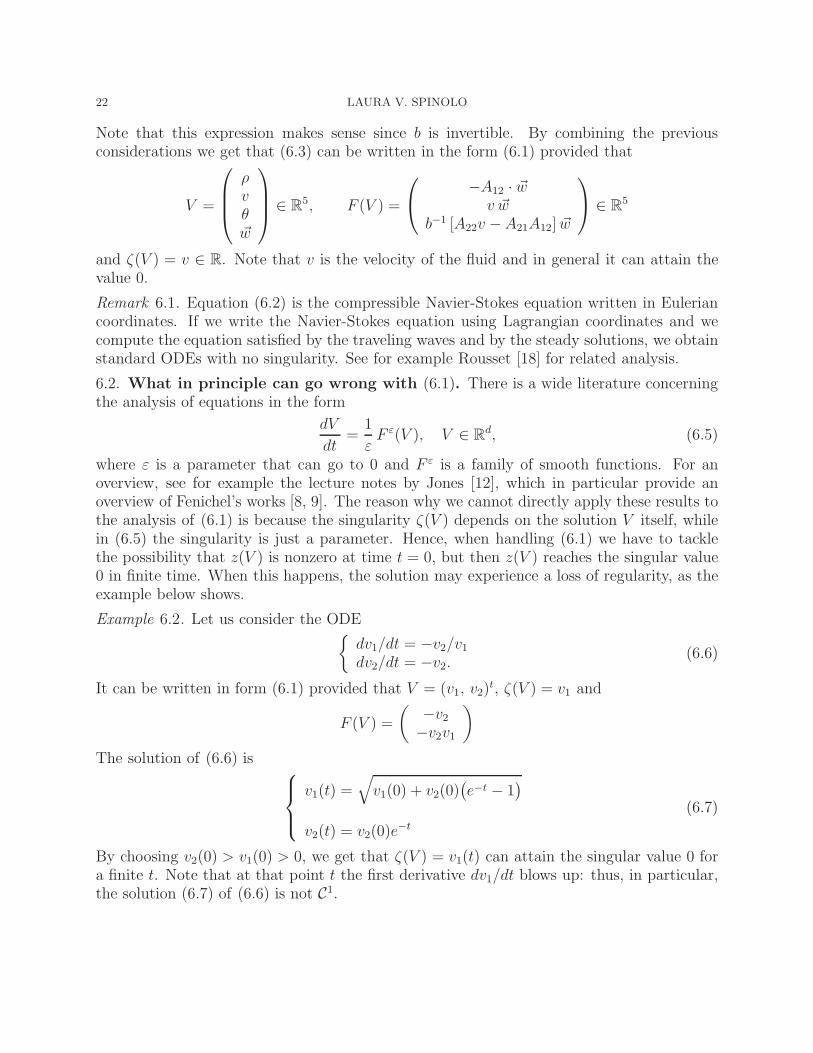
Note that this expression makes sense since b is invertible. By combining the previousconsiderations we get that (6.3) can be written in the form (6.1) provided that

V =

ρvθ~w

∈ R5, F (V ) =

−A12 · ~wv ~w

b−1 [A22v −A21A12] ~w

∈ R5

and ζ(V ) = v ∈ R. Note that v is the velocity of the fluid and in general it can attain thevalue 0.

Remark 6.1. Equation (6.2) is the compressible Navier-Stokes equation written in Euleriancoordinates. If we write the Navier-Stokes equation using Lagrangian coordinates and wecompute the equation satisfied by the traveling waves and by the steady solutions, we obtainstandard ODEs with no singularity. See for example Rousset [18] for related analysis.

6.2. What in principle can go wrong with (6.1). There is a wide literature concerningthe analysis of equations in the form

dV

dt=

1

εF ε(V ), V ∈ R

d, (6.5)

where ε is a parameter that can go to 0 and F ε is a family of smooth functions. For anoverview, see for example the lecture notes by Jones [12], which in particular provide anoverview of Fenichel’s works [8, 9]. The reason why we cannot directly apply these results tothe analysis of (6.1) is because the singularity ζ(V ) depends on the solution V itself, whilein (6.5) the singularity is just a parameter. Hence, when handling (6.1) we have to tacklethe possibility that z(V ) is nonzero at time t = 0, but then z(V ) reaches the singular value0 in finite time. When this happens, the solution may experience a loss of regularity, as theexample below shows.

Example 6.2. Let us consider the ODE{

dv1/dt = −v2/v1

dv2/dt = −v2.(6.6)

It can be written in form (6.1) provided that V = (v1, v2)t, ζ(V ) = v1 and

F (V ) =

(

−v2

−v2v1

)

The solution of (6.6) is

v1(t) =√

v1(0) + v2(0)(

e−t − 1)

v2(t) = v2(0)e−t

(6.7)

By choosing v2(0) > v1(0) > 0, we get that ζ(V ) = v1(t) can attain the singular value 0 fora finite t. Note that at that point t the first derivative dv1/dt blows up: thus, in particular,the solution (6.7) of (6.6) is not C1.


6.3. Goals in studying (6.1). The analysis concerning (6.1) and discussed in the followingaims at applying the ODE techniques described in the previous sections to the study of theviscous profiles of the Navier-Stokes equation.

More precisely, the goals are the following.

(1) Find possible extensions of the Center Manifold Theorem 3.3 and of the UniformlyStable Manifold Theorem 5.2 to the case of the singular ODE (6.1). Note thatboth theorems provide local results, so to study this extension we can restrict to thesolutions of (6.1) belonging to a small enough neighborhood of an equilibrium point.

(2) Rule out the losses of regularity discussed in Example 6.2. To do so, we have to findconditions that guarantee that the following property is satisfied.

If ζ(V ) 6= 0 at t = 0, then ζ(V ) 6= 0 for every t ≥ 0. (6.8)

(3) Impose on (6.1) hypotheses satisfied by the viscous profiles of the Navier-Stokesequation.

6.4. Hypotheses. This section lists the conditions imposed on the functions F and ζ tostudy (6.1), and comments on them.

Hypothesis 1. The functions F : Rd → R

d and ζ : Rd → R are both regular (being of class

C2 is enough). Also, F (~0) = ~0 and ζ(~0) = 0.

The second part of Hypothesis 1 simply says that we are assuming that our equation issingular and that the equilibrium point is ~0, which of course is not restrictive.

Hypothesis 2. We have ∇ζ(~0) 6= ~0.

Let S be the singular setS :=

{

V : ζ(V ) = 0}

.

By relying on the Implicit Function Theorem and on Hypothesis 2 we get that in a smallenough neighbourhood of ~0 the set S is actually a manifold of dimension d − 1, where d isthe dimension of V .

Hypothesis 3. Let Mc be any center manifold for

dV

dτ= F (V ) (6.9)

about the equilibrium point ~0. If |V | is sufficiently small and V belongs to the intersection

Mc ∩ S , then V is an equilibrium for (6.9), namely F (V ) = ~0 .

To understand why we impose Hypothesis 3 let us consider the following simple linearexample.

Example 6.3.

dv1/dτ = v2/εdv2/dτ = −v1/εdε/dτ = 0.

(6.10)

24 LAURA V. SPINOLO

The first component of the solution is

v1(t) = A cos(t/ε) +B sin(t/ε),

where A and B are real parameters. Letting ε → 0+, we get that in general if t 6= 0 thereexists no pointwise limit of v1. Note that (6.10) does not satisfy Hypothesis 3. Indeed, thecenter space is the whole R

3 and it coincides with the center manifold. However,

F (V ) =

v2

−v1

0

is not identically zero when ε = 0.

We now assume that there exists a non-degenerate set of equilibria.

Hypothesis 4. There exists a one-dimensional manifold of equilibria E for the equation

dV

dτ= F (V )

which contains ~0 and which is transversal to S.

The one-dimensional manifold E is transversal to the manifold S if the intersection S∩Meq

has dimension zero.

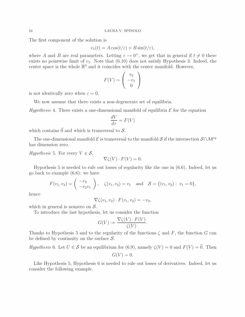
Hypothesis 5. For every V ∈ S,∇ζ(V ) · F (V ) = 0.

Hypothesis 5 is needed to rule out losses of regularity like the one in (6.6). Indeed, let usgo back to example (6.6): we have

F (v1, v2) =

(

−v2

−v2v1

)

, ζ(v1, v2) = v1 and S = {(v1, v2) : v1 = 0},

hence∇ζ(v1, v2) · F (v1, v2) = −v2,

which in general is nonzero on S.To introduce the last hypothesis, let us consider the function

G(V ) :=∇ζ(V ) · F (V )

ζ(V ).

Thanks to Hypothesis 5 and to the regularity of the functions ζ and F , the function G canbe defined by continuity on the surface S.

Hypothesis 6. Let U ∈ S be an equilibrium for (6.9), namely ζ(V ) = 0 and F (V ) = ~0. Then

G(V ) = 0.

Like Hypothesis 5, Hypothesis 6 is needed to rule out losses of derivatives. Indeed, let usconsider the following example.


Example 6.4. Let us consider the ODE

dv1/dt = −v3

dv2/dt = −v2/v1

dv3/dt = −v3,(6.11)

then we can set

F (v1, v2, v3) =

−v3v1

−v2

−v3v1

, ζ(v1, v2, v3) = v1 and S = {(v1, v2, v3) : v1 = 0},

so that

∇ζ · F = −v3v1 = 0 on Sand hence Hypothesis 5 is satisfied. As a matter of fact, one can verify that Hypotheses 1 . . . 4are all satisfied as well. However, Hypothesis 6 is violated: indeed,

G(v1, v2, v3) = −v3,

which is in general different from 0 on{

(v1, v2, v3) : such that F (v1, v2, v3) = ~0 and ζ(v1, v2, v3) = 0}

={

(0, 0, v3)}

.

By solving (6.11) explicitly we get, after some computations,

v1(t) = v1(0)(1 − A) + Av1(0)e−t

v2(t) = B[

(1 − A)et + A]

[

(A−1)v1(0)]

−1

v3(t) = Av1(0)e−t,

where A and B are suitable constants depending on the initial data. If (A−1)v1(0) > 1, thenthe first derivative dv2/dt blows up at t = ln(A/A−1). Note that this is exactly the value oft at which v1(t) attains 0. In general, for every v1(0) > 0 if 1/(A− 1)v1(0) is not a naturalnumber, then the solution is not in Cm for m = [1/(A− 1)v1(0)] + 1. Here [1/(A− 1)v1(0)]denotes the entire part. Thus, we have a loss of regularity in higher derivatives.

Remark 6.5. One can verify that Hypotheses 1. . . 6 are all verified by the viscous profiles(travelling waves and steady solutions) of the Navier Stokes equation (6.2).

6.5. A toy model. To get a flavor of the behaviors we expect to encounter, we start byconsidering the case when the singularity is only a parameter. Actually, to simplify thingswe focus on a toy model where everything is linear and we can carry out the computationsexplicitly. Let us consider the system

dv1/dt = −5v1

dv2/dt = −v2/εdε/dt = 0.

(6.12)

26 LAURA V. SPINOLO

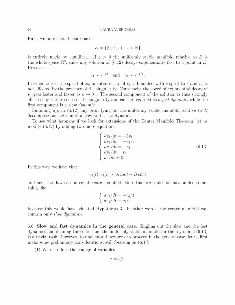
First, we note that the subspace

E = {(0, 0, ε) : ε ∈ R}

is entirely made by equilibria. If ε > 0 the uniformly stable manifold relative to E isthe whole space R

3, since any solution of (6.12) decays exponentially fast to a point in E.However,

v1 ∼ e−5t and v2 ∼ e−t/ε.

In other words, the speed of exponential decay of v1 is bounded with respect to ε and v1 isnot affected by the presence of the singularity. Conversely, the speed of exponential decay ofv2 gets faster and faster as ε → 0+. The second component of the solution is thus stronglyaffected by the presence of the singularity and can be regarded as a fast dynamic, while thefirst component is a slow dynamic.

Summing up, in (6.12) any orbit lying on the uniformly stable manifold relative to Edecomposes as the sum of a slow and a fast dynamic.

To see what happens if we look for extensions of the Center Manifold Theorem, let usmodify (6.12) by adding two more equations:

dv1/dt = −5v1

dv2/dt = −v2/εdv3/dt = −v4

dv4/dt = v3

dε/dt = 0.

(6.13)

In this way, we have that

v3(t), v4(t) ∼ A cos t+B sin t

and hence we have a nontrivial center manifold. Note that we could not have added some-thing like

{

dv3/dt = −v4/εdv4/dt = v3/ε

because this would have violated Hypothesis 3. In other words, the center manifold cancontain only slow dynamics.

6.6. Slow and fast dynamics in the general case. Singling out the slow and the fastdynamics and defining the center and the uniformly stable manifold for the toy model (6.13)is a trivial task. However, to understand how we can proceed in the general case, let us firstmake some preliminary considerations, still focusing on (6.13).

(1) We introduce the change of variables

τ = t/ε.


Then (6.13) becomes

dv1/dτ = −5v1εdv2/dτ = −v2

dv3/dτ = −v4εdv4/dτ = v3εdε/dτ = 0.

(6.14)

(2) We can single out the slow dynamics of (6.13) by considering the center spaceof (6.14), which is given by {(v1, 0, v3, v4, ε)}.

(3) Let us now restrict the analysis to the center space of (6.14): we obtain

dv1/dτ = −5v1εdv3/dτ = −v4εdv4/dτ = v3εdε/dτ = 0.

Hence, we can come back to the original variable t, obtaining an equation with nosingularity in it:

dv1/dt = −5v1

dv3/dt = −v4

dv4/dt = v3

dε/dt = 0.

(6.15)

(4) We can then consider the center space of (6.15), which is given by V c = {(0, v3, v4, ε)}.Then the center manifold of the original system (6.13) is exactly V c. Also, we canobserve that E = {(0, 0, 0, ε)} is a subspace of equilibria for (6.15) and we can considerthe uniformly stable space of (6.15) with respect to E: it is given by {(v1, 0, 0, ε)}.

(5) Let us now consider the uniformly stable manifold of (6.13) with respect to themanifold of equilibria E = {(0, 0, 0, ε)}. It is given by {(v1, v2, 0, 0, ε)} : as mentionedbefore, any solution in there writes as a fast dynamic (in this case, (0, v2, 0, 0)) plusa slow dynamic (in this case, (v1, 0, 0, ε)) belonging to the uniformly stable manifoldof (6.15) with respect to E.

Let us now discuss how one can proceed in the general case

dV

dt=

1

ζ(V )F (V ). (6.16)

Actually, we will not enter into the technical details, which can be found in [4]. The heuristicidea is proceeding by following the same steps (1). . . (5) as in the case of the toy model. Ofcourse, now we have to handle additional difficulties coming from the fact that there is anon linearity in the function F (V ). Also, ζ(V ) is no more a parameter, but depends on thesolution itself, and hence we have to rule out the possibility that ζ(V ) 6= 0 at t = 0 but ζ(V )reaches 0 in finite time.

28 LAURA V. SPINOLO

Actually, as a preliminary step it is convenient to introduce a change of coordinates whichallows to write (6.16) in a more convenient form, however, this is a mostly technical stepand in here we do not go into the details (they can be found in [4, Proposition 4.1]).

Let us now informally discuss how to extend the previous steps to the general case (6.16).

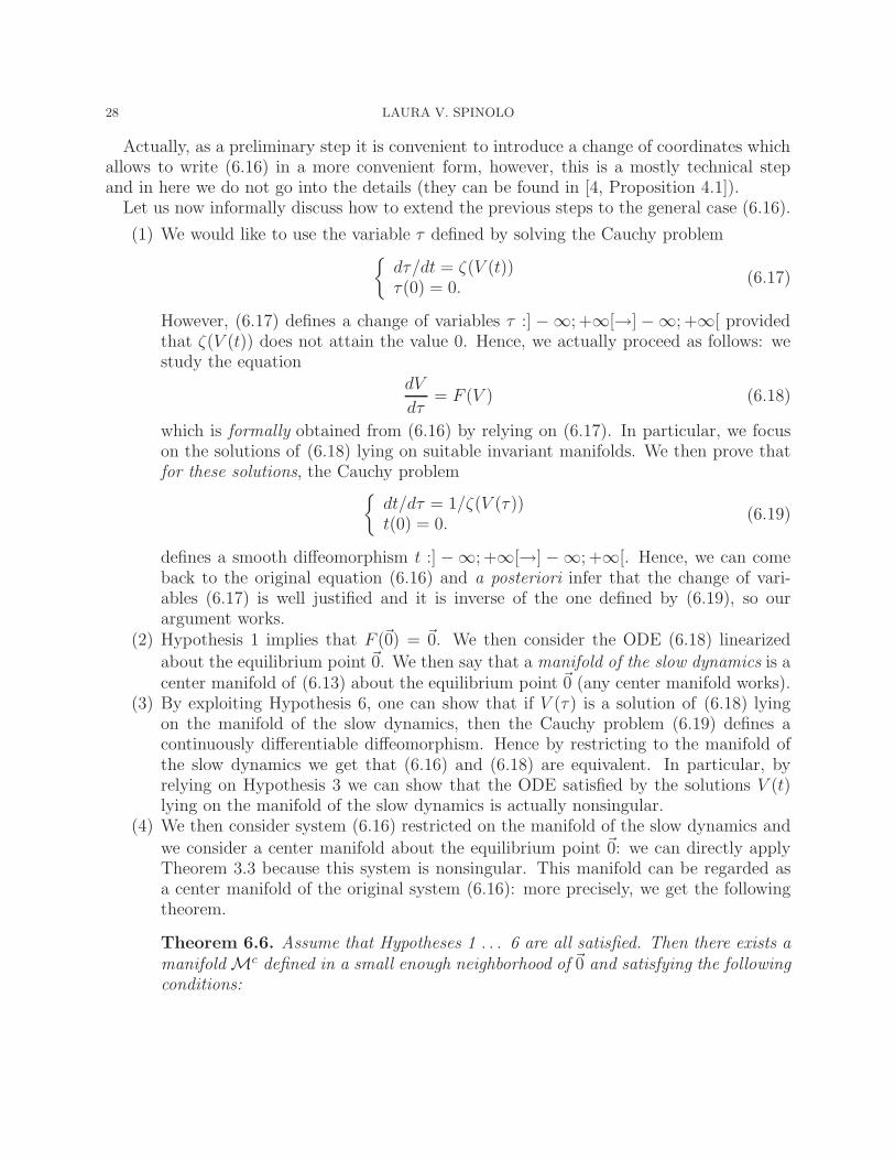
(1) We would like to use the variable τ defined by solving the Cauchy problem{

dτ/dt = ζ(V (t))τ(0) = 0.

(6.17)

However, (6.17) defines a change of variables τ :] −∞; +∞[→] −∞; +∞[ providedthat ζ(V (t)) does not attain the value 0. Hence, we actually proceed as follows: westudy the equation

dV

dτ= F (V ) (6.18)

which is formally obtained from (6.16) by relying on (6.17). In particular, we focuson the solutions of (6.18) lying on suitable invariant manifolds. We then prove thatfor these solutions, the Cauchy problem

{

dt/dτ = 1/ζ(V (τ))t(0) = 0.

(6.19)

defines a smooth diffeomorphism t :] −∞; +∞[→] −∞; +∞[. Hence, we can comeback to the original equation (6.16) and a posteriori infer that the change of vari-ables (6.17) is well justified and it is inverse of the one defined by (6.19), so ourargument works.

(2) Hypothesis 1 implies that F (~0) = ~0. We then consider the ODE (6.18) linearized

about the equilibrium point ~0. We then say that a manifold of the slow dynamics is acenter manifold of (6.13) about the equilibrium point ~0 (any center manifold works).

(3) By exploiting Hypothesis 6, one can show that if V (τ) is a solution of (6.18) lyingon the manifold of the slow dynamics, then the Cauchy problem (6.19) defines acontinuously differentiable diffeomorphism. Hence by restricting to the manifold ofthe slow dynamics we get that (6.16) and (6.18) are equivalent. In particular, byrelying on Hypothesis 3 we can show that the ODE satisfied by the solutions V (t)lying on the manifold of the slow dynamics is actually nonsingular.

(4) We then consider system (6.16) restricted on the manifold of the slow dynamics and

we consider a center manifold about the equilibrium point ~0: we can directly applyTheorem 3.3 because this system is nonsingular. This manifold can be regarded asa center manifold of the original system (6.16): more precisely, we get the followingtheorem.

Theorem 6.6. Assume that Hypotheses 1 . . . 6 are all satisfied. Then there exists amanifold Mc defined in a small enough neighborhood of ~0 and satisfying the followingconditions:


(a) if U(t) is a solution of (6.16) lying on Mc and ζ(V ) 6= 0 at t = 0 then ζ(V ) 6= 0for every t ∈ R.

(b) Mc s locally invariant for (6.16). Namely, if V ∈ Mc, then the solution of theCauchy problem

dV

dt=

1

ζ(V )F (V )

V (0) = V

satisfies V (t) ∈ Mc for |t| small enough.(c) There exists a small enough constant δ > 0 such that the following holds. If V (t)

is a solution of (6.16) satisfying |V (t)| ≤ δ for every t ∈ R, then V (t) ∈ Mc.

Remark 6.7. In the statement of the Center Manifold Theorem 3.3 and of the Uni-formly Stable Manifold Theorem 5.2 one assumes that suitable subspaces (the centerand the stable subspace, respectively) are non trivial. One should actually add ananalogous condition to the statement of Theorem 6.6. However, to simplify the no-tations we can use the convention that [F (~0)/ζ(~0)] = ~0/0 := ~0 and that if a subspace

is trivial then any manifold parameterized by this subspace is just the origin ~0. Withthese conventions the statement of Theorem 6.6 is formally correct. We will adoptthe same convention in the statements of Theorem 6.8.

(5) We now want find an extension of the Uniformly Stable Manifold Theorem. First,we recall that Hypothesis 4 ensures that there is a manifold of equilibria E for (6.18)which is transversal to the hypersurface {V : ζ(V ) = 0}. One can show that thepoints of E are also equilibria for system (6.16) restricted on the manifold of the slowdynamics.

By relying on the analogy with the toy model, we would like to define a manifoldMus such that any solution lying on Mus decays exponentially fast to some point inE . Also, any orbit lying on Mus should be written as the sum of a fast dynamic andof some stable component coming from the slow dynamics. However, since we are inthe non linear case we expect some interactions between the different components.The precise result is the following.

Theorem 6.8. Let Hypotheses 1. . . 6 hold and denote by E the same manifold ofequilibria as in Hypothesis 4. Then there exist a constant c > 0 and a manifoldMus which is defined in a small enough neighborhood of ~0 and satisfies the followingconditions.(a) If V (t) is a solution of (6.16) lying on Mus and ζ(V ) 6= 0 at t = 0 then ζ(V ) 6= 0

for every t ≥ 0.

30 LAURA V. SPINOLO

(b) Mus is locally invariant for (6.16). Namely, if V ∈ Mus, then the solution ofthe Cauchy problem

dV

dt=

1

ζ(V )F (V )

V (0) = V

satisfies V (t) ∈ Mus for |t| small enough.(c) If V (t) lies on Mus then there exists V∞ ∈ E such that

limt→+∞

|V (t) − V∞|ect = 0.

(d) If V (t) lies on Mus then

V (t) = Vsl(t) + Vf(t) + Vp(t),

where Vsl lies on the manifold of the slow dynamics and Vf satisfies

limτ→+∞

|Vf(τ)|ecτ = 0.

Here the variable τ is defined by solving the Cauchy problem (6.19). Finally,Vp is an interaction term which is small with respect to the previous two (in thesense specified in the statement of [4, Theorem 4.2]).

The proof of Theorem 6.8 relies on the following lemma of standard flavor.

Lemma 6.9. Consider the ODE

dV

dτ= F (V ) (6.20)

and assume that Hypothesis 1 is satisfied and that the center and the stable spaceabout the equilibrium point ~0 are both non-trivial . Let S0 be a submanifold of acenter manifold of (6.20) about the equilibrium point ~0. Also, assume that S0 islocally invariant for (6.20). Then there exists a constant c > 0 and a manifold Mwhich is defined in a small enough neighborhood of ~0, is locally invariant for (6.20)and satisfies the following properties. If V (τ) lies on M then

V (τ) = V0(τ) + Vf(τ) + Vp(τ),

where V0 lies on S0 and Vf satisfies

limτ→+∞

|Vf(τ)|ecτ = 0.

Moreover, Vp is an interaction term which is small with respect to the previous two(in the sense specified in the statement of [4, Proposition 3.1]).


Note that, in particular, the statement of Lemma 6.9 ensures that any solutionlying on M becomes exponentially close to an orbit on S0 and hence M can beregarded as a slaving manifold for S0. The proof of Lemma 6.9 is a bit technical, butit can be obtained by relying on a fixed point argument.

Toward a proof of Theorem 6.8, one first defines S0 as follows. Consider therestriction of (6.16) to the manifold of the slow dynamics: as pointed out before,this system is non singular and E is a manifold of equilibria. Hence, one can directlyapply the Uniformly Stable Manifold Theorem 5.2 and define S0 as the uniformlystable manifold relative to E of system (6.16) restricted to the manifold of the slowdynamics. By applying Lemma 6.9 and by relying on some more work one can thenconclude the proof of Theorem 6.8.

References

[1] Ancona, F., and Bianchini, S. Vanishing viscosity solutions of hyperbolic systems of conservationlaws with boundary. In “WASCOM 2005”—13th Conference on Waves and Stability in ContinuousMedia. World Sci. Publ., Hackensack, NJ, 2006, pp. 13–21.

[2] Bianchini, S. On the Riemann Problem for Non-Conservative Hyperbolic Systems. Arch. RationalMech. Anal. 166, 1 (2003), 1–26.

[3] Bianchini, S., and Bressan, A. Vanishing viscosity solutions of non linear hyperbolic systems. Ann.of Math. 161 (2005), 223–342.

[4] Bianchini, S., and Spinolo, L. V. Invariant manifolds for a singular ordinary differential equation.Submitted. Also arXiv:0801.4425.

[5] Bianchini, S., and Spinolo, L. V. The boundary Riemann solver coming from the real vanishingviscosity approximation. Arch. Rational Mech. Anal. 191, 1 (2009), 1–96.

[6] Bressan, A., Serre, D., Williams, M., and Zumbrun, K. Hyperbolic systems of balance laws,vol. 1911 of Lecture Notes in Mathematics. Springer, Berlin, 2007. Lectures given at the C.I.M.E.Summer School held in Cetraro, July 14–21, 2003. Edited and with a preface by Pierangelo Marcati.

[7] Dafermos, C. M. Hyperbolic Conservation Laws in Continuum Physics, Second ed. Springer-Verlag,Berlin 2005.

[8] Fenichel, N. Asymptotic stability with rate conditions. Indiana Univ. Math. J. 23 (1973/74), 1109–1137.

[9] Fenichel, N. Geometric singular perturbation theory for ordinary differential equations. J. DifferentialEquations 31, 1 (1979), 53–98.

[10] Gisclon, M. Etude des conditions aux limites pour un systeme hyperbolique, via l’approximationparabolique. J. Maths. Pures & Appl. 75 (1996), 485–508.

[11] Glimm, J. Solutions in the large for nonlinear hyperbolic systems of equations. Comm. Pure Appl.Math. 18 (1965), 697–715.

[12] Jones, C. R. T. Geometric singular perturbation theory. In Dynamical systems (Montecatini Terme,1994), vol. 1609 of Lecture Notes in Math. Springer, Berlin 1995, pp. 44–118.

[13] Joseph, K. T., and LeFloch, P. G. Singular limits for the riemann problem: general diffusion, re-laxation, and boundary conditions. In O. Rozanova, Editor, Analytical Approaches to MultidimensionalBalance Laws. Nova Publishers 2005.

[14] Katok, A., and Hasselblatt, B. Introduction to the modern theory of dynamical systems, vol. 54 ofEncyclopedia of Mathematics and its Applications. Cambridge University Press, Cambridge, 1995. Witha supplementary chapter by Katok and Leonardo Mendoza.

[15] Lax, P. Hyperbolic systems of conservation laws II. Comm. Pure Appl. Math. 10 (1957), 537–566.

32 LAURA V. SPINOLO

[16] Liu, T. P. The Riemann Problem for General Systems of Conservation Laws. J. Differential Equations18 (1975), 218–234.

[17] Perko, L. Differential Equations and Dynamical Systems, third ed., vol. 7. Springer-Verlag, New York2001.

[18] Rousset, F. Characteristic boundary layers in real vanishing viscosity limits. J. Differential Equations210 (2005), 25–64.

[19] Serre, D. Systems of Conservation Laws, I, II. Cambridge University Press, Cambridge 2000.[20] Tzavaras, A. E. Wave interactions and variation estimates for self-similar zero-viscosity limits in

systems of conservation laws. Arch. Rational Mech. Anal. 135, 1 (1996), 1–60.

Centro De Giorgi, Collegio Puteano, Scuola Normale Superiore, Piazza dei Cavalieri 3,

56126 Pisa, Italy

E-mail address : [email protected]

Date post:	22-Feb-2019
Category:	Documents
Upload:	vanthu
View:	233 times
Download:	0 times

Introduction - user.math.uzh.chuser.math.uzh.ch/spinolo/notes.pdf · LAURA V. SPINOLO Abstract....

Documents