Inverse Probability of Autopsy Weighting – Moving Toward Best Practices Erin L. Abner, PhD, MPH Taylor G. Estepp, MS Alzheimer’s Disease Research Center Sanders-Brown Center on Aging College of Public Health
Transcript
Inverse Probability of Autopsy Weighting –
Moving Toward Best PracticesErin L. Abner, PhD, MPH
Taylor G. Estepp, MS
Alzheimer’s Disease Research CenterSanders-Brown Center on Aging
College of Public Health
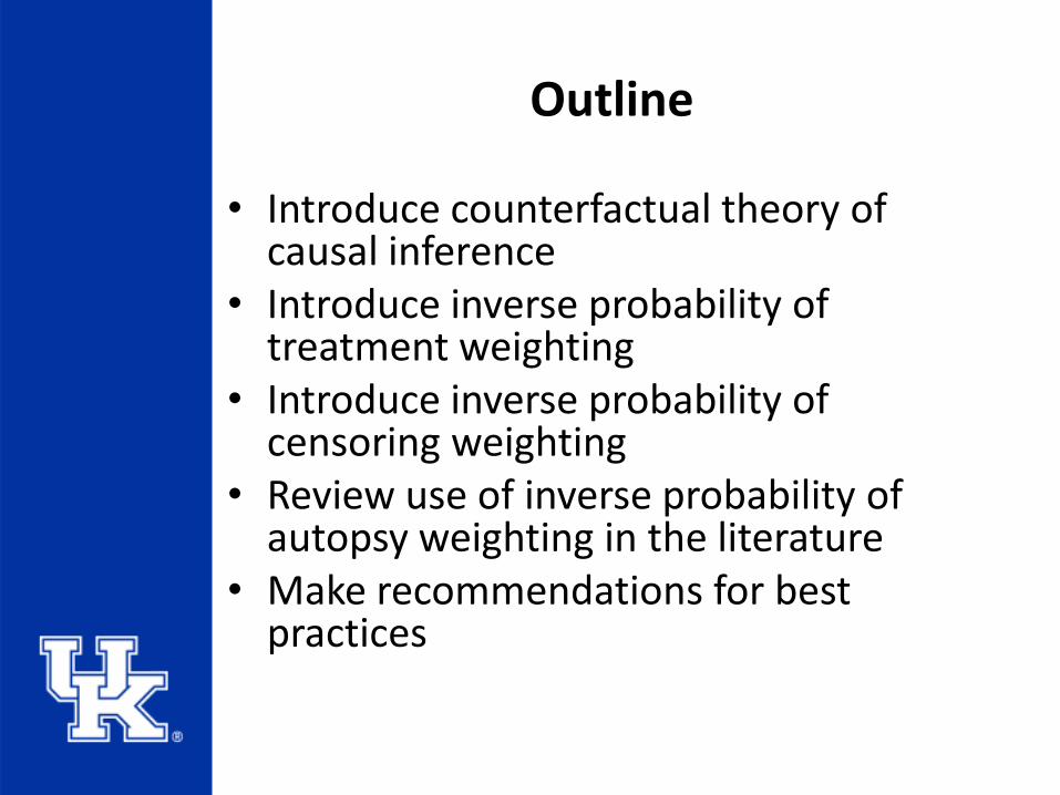
Outline
• Introduce counterfactual theory of causal inference
• Introduce inverse probability of treatment weighting
• Introduce inverse probability of censoring weighting
• Review use of inverse probability of autopsy weighting in the literature
• Make recommendations for best practices
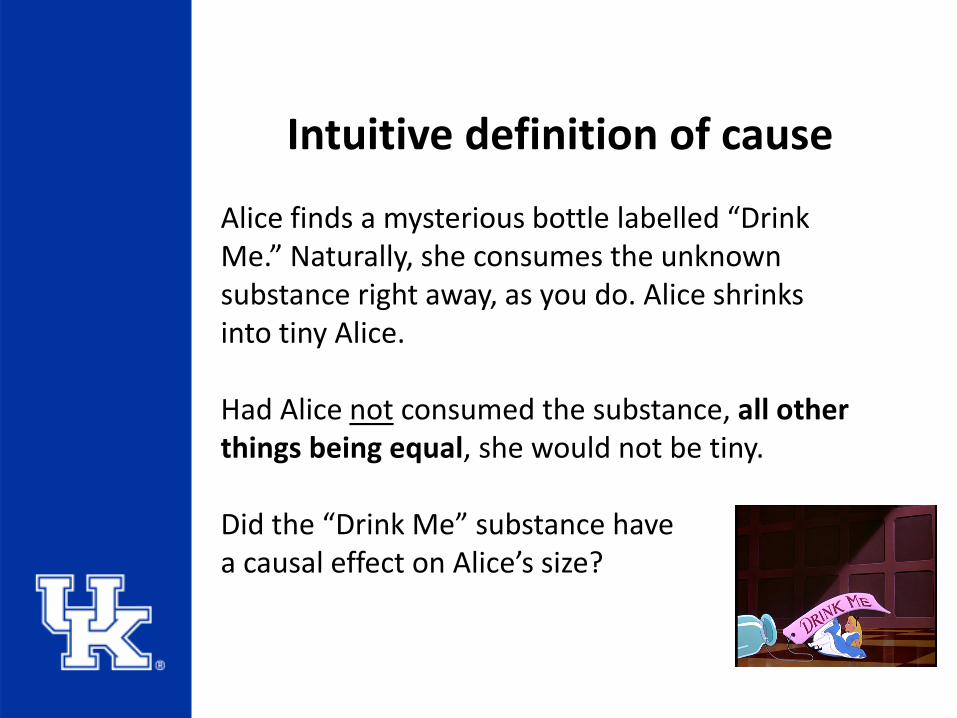
Intuitive definition of cause
Alice finds a mysterious bottle labelled “Drink Me.” Naturally, she consumes the unknown substance right away, as you do. Alice shrinks into tiny Alice.
Had Alice not consumed the substance, all other things being equal, she would not be tiny.
Did the “Drink Me” substance have a causal effect on Alice’s size?
Counterfactual Theory
• We define the relationship between an exposure/treatment/intervention and an outcome as “causal” when the potential outcomes under the treatment are not equal
• Potential outcomes may be written as YA=a, which is interpreted as the value of Y when treatment takes the value “a”
• Thus, YA=a ≠ YA≠a is interpreted to mean there is a causal effect of treatment A on outcome Y
Fundamental problem of causal inference
• We can only observe one potential outcome for any individual, the one corresponding to their observed treatment (SUTVA)
• We cannot evaluate YA=a ≠ YA≠a for any individual
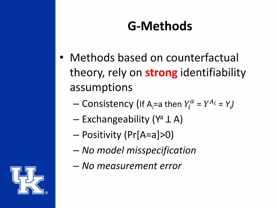
G-Methods
• Methods based on counterfactual theory, rely on strong identifiability assumptions– Consistency (If Ai=a then 𝑌𝑌𝑖𝑖𝑎𝑎 = 𝑌𝑌𝐴𝐴𝑖𝑖 = Yi)
– Exchangeability (Ya ꓕ A)– Positivity (Pr[A=a]>0)– No model misspecification– No measurement error
• Addresses unequal probabilities of treatment in observational studies
• Observations are weighted by their conditional (on L) probability of receiving treatment A=a
• Unlike prediction modeling, the goal is not to find the model with the smallest residual; goal is identify the set L
IPT Weights
• Observations are weighted by the inverse of the conditional probability of their observed treatment: WA=1/(f(A|L)
• Stabilized weights are recommended: SWA=f(A)/(f(A|L)
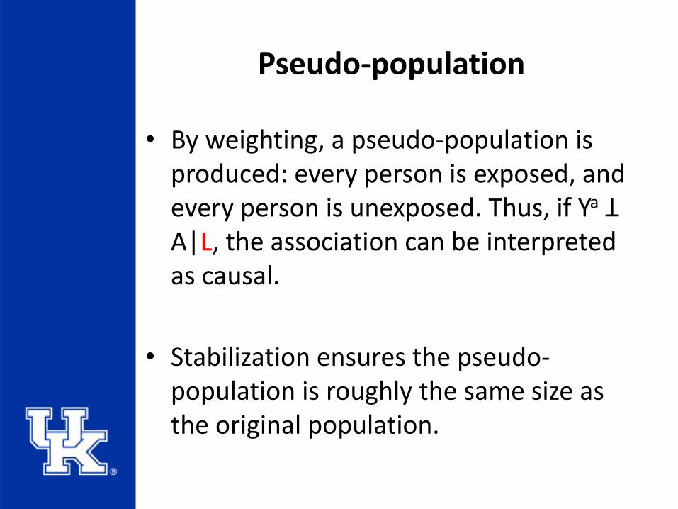
Pseudo-population
• By weighting, a pseudo-population is produced: every person is exposed, and every person is unexposed. Thus, if Ya ꓕA|L, the association can be interpreted as causal.
• Stabilization ensures the pseudo-population is roughly the same size as the original population.
Selection Bias
• In addition to confounding, observational studies are plagued by selection biases
• Occurs when we condition on a common effect of two variables, one of which is the treatment or is associated with the treatment, andone of which is the outcome or associated with the outcome
(Over-simplified) causal diagram depicting hypothesized causal relation between Braak stage and dementia; since Braak stage cannot be observed without autopsy, we are forced to condition on autopsy, which introduces selection bias
(Still over-simplified) causal diagram depicting hypothesized causal relation between Braak stage and dementia status
IPCW
• Goal is either: – to create a pseudo-population that
represents the entire uncensored original population before censoring
– or, to create a pseudo-population the same size as the uncensored population, but without selection bias (stabilized IPCW)
• Often, the causal estimand we are really interested in is: E[Ya=1,c=0] - E[Ya=0,c=0] = E[Y|C=0,A=1,L=l] –E[Y|C=0,A=0,L=l]
• In our case, we want to know what the association is in a world where either everyone is autopsied, or autopsy occurs at random
Joint Weights
• We can address confounding and selection bias by computing treatment weights and censoring weights, and taking their product
• IPW is a powerful analytic tool!
With great power…
comes great responsibility
IPW Best Practices
• IPW is only valid if the assumptions hold• Assess consistency assumption
– Outside the data; based on expert knowledge• Assess exchangeability
– Directed acyclic graphs– Examine distribution of weights– Evaluation of weighted data for balance
• Assess positivity– Based on the data; expert knowledge
Inverse Probability of Autopsy Weights
• Introduced by Haneuse et al., 2009• Applied IPAW to autopsied ACT
participants • Used in at least 8 published studies
since, usually ACT or NACC data
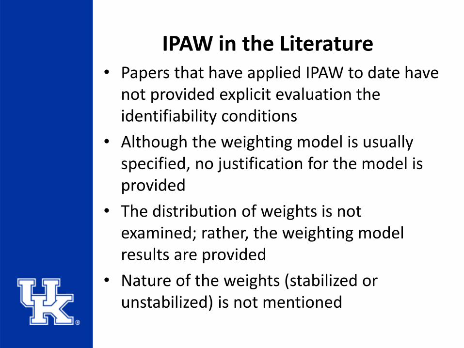
IPAW in the Literature• Papers that have applied IPAW to date have
not provided explicit evaluation the identifiability conditions
• Although the weighting model is usually specified, no justification for the model is provided
• The distribution of weights is not examined; rather, the weighting model results are provided
• Nature of the weights (stabilized or unstabilized) is not mentioned
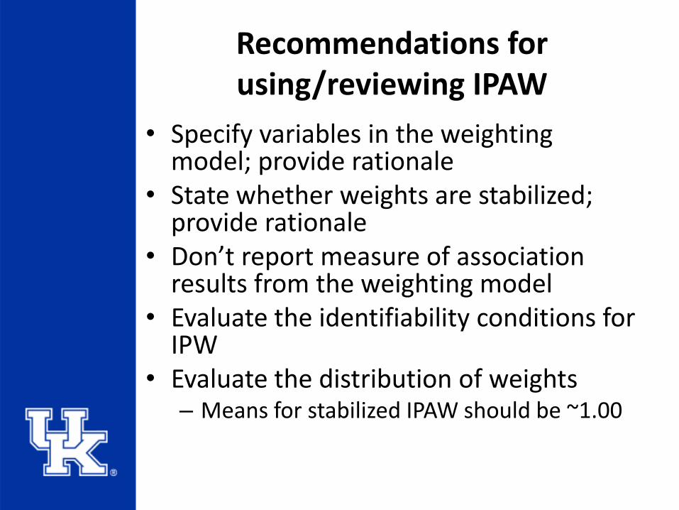
Recommendations for using/reviewing IPAW
• Specify variables in the weighting model; provide rationale
• State whether weights are stabilized; provide rationale
• Don’t report measure of association results from the weighting model
• Evaluate the identifiability conditions for IPW
• Evaluate the distribution of weights– Means for stabilized IPAW should be ~1.00
Summary• The nature of clinico-pathologic studies
means we must condition on a common effect of the exposure and outcome, which induces selection bias
• IPAW is appealing tool to mitigate this selection bias
• But, IPAW is based on very strong assumptions that must be evaluated each time it is used
• Careful assessment and reporting of these assumptions will increase the rigor of our research
Thank you!
This work was partially supported by NIA R01AG038651 and P30AG028383.