Investigation of advanced data processing technique in...

INVESTIGATION OF ADVANCED DATA PROCESSING

TECHNIQUE IN MAGNETIC ANOMALY DETECTION

SYSTEMS

B. Ginzburg(1), L. Frumkis(2), B.Z. Kaplan(2), A. Sheinker(1,2), N. Salomonski(1)

(1) Soreq NRC, Yavne, 81800, Israel, [email protected] (2) Ben-Gurion University of the Negev, P.O. Box 653, Beer-Sheva, 84105, Israel

Abstract - Advanced methods of data processing in magnetic anomaly detection (MAD) systems are

investigated. Raw signals of MAD based on component magnetic sensors are transformed into

energy signals in the space of specially constructed orthonormalized functions. This procedure

provides a considerable improvement of the SNR thus enabling reliable target detection. Estimation

of the target parameters is implemented with the help of Genetic Algorithm. Numerous computer

simulations show good algorithm convergence and acceptable accuracy in estimation of both target

location and its magnetic moment.

Index terms: Magnetometer, Magnetic Anomaly Detection, Orthonormal basis, Genetic algorithm

I. INTRODUCTION

The necessity to detect hidden ferromagnetic subjects (e.g. mines, underwater wrecks, and

sunken ships etc) has led to several detection techniques, one of which is the Magnetic

Anomaly Detection (MAD). The principle of the MAD is based on the ability to sense the

anomaly in Earth magnetic field produced by the target. [1-3]

There are two basic types of MAD: search and alarm systems. In the first case, magnetic

sensors are installed on the moving platform searching for hidden ferromagnetic target by

surveying specific area along predefined paths (usually straight lines). Target presence is

revealed as a spatial magnetic anomaly along the survey line passing in the vicinity of the

target. MAD of alarm type makes use of stationary instruments producing an alarm signal

when ferromagnetic target passes nearby the magnetic sensor. We assume the distance

between the target and the sensor noticeably exceeding target dimensions so that target

magnetic field is described by dipole model. MAD signal is time-depending magnetic field

110

INTERNATIONAL JOURNAL ON SMART SENSING AND INTELLIGENT SYSTEMS, VOL. 1, NO. 1, MARCH 2008

caused by mutual motion of magnetic dipole and the sensor. Therefore, our approach to signal

processing is equally applicable for both types of MAD systems.

Magnetometers of various types are widely used for detection and characterization of hidden

ferromagnetic objects by analyzing small Earth’s magnetic field anomalies. The basic

problem, which arises when measuring weak magnetic field anomalies, is a problem of small

signal detection and estimation of target parameters in the presence of noise and interference.

In the present work we analyze different signal processing methods for MAD based on vector

magnetic sensors. Our investigation covers two basic types of such sensors, where the first

one (e.g. fluxgate) provides a direct reading of a field component and the second one (search

coil in low-frequency mode) responds to time-derivative of magnetic field.

II. PRESENTATION OF FIELD COMPONENT SIGNALS WITH THE AID OF

ORTHONORMAL FUNCTIONS

Let magnetic dipole whose moment components are Mx, My and Mz is located at the origin of

the X, Y, Z coordinate system. The line of the sensor platform movement is parallel to the X

axis. Each of three mutually orthogonal component sensors is aligned in parallel to one of the

coordinate axes (Fig. 1).

Sensors

Z

MxMy

Mz

Line of sensors movement

h

s

A(x,s,h)

R M

X

Y

R0

Figure1. Relative position of the magnetic dipole M and the sensors.

The distance between the line of the sensor movement and the Z axis is s, and the distance

between this line and the XY plane is h. R0 is the distance between the dipole and the line of the

sensor movement. It is the so-called CPA (closest proximity approach) distance, 22

0 hsR += (1)

111

B. GINZBURG ET., AL., INVESTIGATION OF ADVANCED DATA PROCESSING TECHNIQUE IN MAGNETIC ANOMALY DETECTION SYSTEMS

The magnetic field B generated by a point dipole with a moment M at some distance R from

the dipole is

])(3[4

230 M-RRMB ⋅= −− RRπμ (2)

where μ0= 4π⋅10-7 H/m is the permeability of free space.

Equation (2) can be rewritten in matrix form (see, for instance, [4])

(3) zMRB 333

4−

π y

x

z

y

x

MM

zzyzxyzRyyxxzxyRx

RBB

22

22

22

50 333

333−

−=

μ

and after normalizing,

(4) 0/ Rxw =

(5) ,/ MMm zz =,/ MMm xx = ,/ MMm yy =

222zyx MMMM ++=

(6) 01 /3 Rsa = 02 /3 Rha = 20

23 /3 Rsa = 2

04 /3 Rsha = 20

25 /3 Rha =

Equation (3) takes the form:

z

y

x

z

y

x

mmm

wwawawawawwawawawaww

RM

BBB

)()()()()()()()()()()()(3

41252432

2412331

323114

30

0

ϕϕϕϕϕϕϕϕϕϕϕϕ

π

μ

−−

−=

(7)

where 5.121 )1()( −+= wwϕ 5.22

2 )1()( −+= wwϕ (8)

5.223 )1()( −+= wwwϕ ( ) 5.222

4 1)( −+= wwwϕ

Functions ϕ 1(w), ϕ 2(w) and ϕ 3(w) are linearly independent, while ϕ 4(w) can be excluded

basing on

(9) )()()( 214 www ϕϕϕ −=

112


Applying Gram-Schmidt orthonormalization procedure [5] we get triplet of mutually

orthogonal functions F1(w), F2(w), and F3(w):

5.121 )1(

38)( −+= wwFπ

])1(65)1[(

5384)( 5.125.22

2−− +−+= wwwF

π

(10)

5.22

3 )1(5π128)( −+= wwwF

satisfying usual orthonormalization conditions:

113

3

2

1

FFF

ABBB

z

y

x

⋅=

0)()(∫+∞

∞

=dwwFwF ji 1)(2∫+∞

∞−

=dwwFj for ji , and , i, j = 1, 2, 3. (11) ≠−

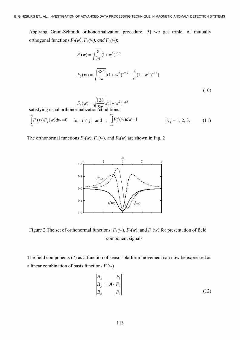
The orthonormal functions F1(w), F2(w), and F3(w) are shown in Fig. 2

-4 -2 0 2 4

-1.0

-0.5

0.0

0.5

1.0

F3(w)

F2(w)F1(w)

w

Figure 2.The set of orthonormal functions: F1(w), F2(w), and F3(w) for presentation of field

component signals.

The field components (7) as a function of sensor platform movement can now be expressed as

a linear combination of basis functions Fi(w)

(12)


where A is 3x3 matrix which coefficients depend on a particular dipole position and

orientation and may be obtained in the following way:

∫=∞

∞−dwwBwFA jiij )()( i=1, 2, 3; j=x, y, z (13)

It is important to underline that (12, 13) keep true not only for any dipole position and

orientation but for any direction of sensor platform and its orientation as well. This enables us

with an opportunity to implement unified algorithm for processing of MAD signal as it would

be shown below.

It is worthy to note that basic functions (10) coincide with the same functions which can be

employed for the case of MAD based on scalar magnetometer [6, 7].

III. PRESENTATION OF TIME DERIVATIVES OF FIELD COMPONENT WITH

THE AID OF ORTHONORMAL FUNCTIONS

Search-coil magnetometers are widely used for component measurements in MAD systems.

For direct mode of operation the output signal of search-coil magnetometer is proportional to

the ambient field. For that case all results of previous section are applicable. The direct mode

of operation is usually a result of relatively large self capacitance of the coil windings, and/or

electronics correction measures. However, in the lower part of operation frequency band

search coil sensor operates in derivative mode [8]. In this case sensor signals Sx,y,z can be

written as

dwdB

RVK

dtdx

dxdw

dwdB

Kdt

dBKS zyxzyxzyx

zyx,,

0

,,,,,, ===

(14)

where K is coefficient depending on permeability of search-coil core, number of turns, and

coil geometry, while V is the velocity of the sensor platform. Implementing mathematical

transformations like in previous section it is easy to show that signals of search-coil

magnetometers (14) can be presented by linear combination of four functions

5.221 )1()( −+= wwwψ , 5.32

2 )1()( −+= wwwψ , 5.323 )1()( −+= wwψ ,

(15)

5.3224 )1()( −+= wwwψ

114


After implementation of Gram-Schmidt procedure we get quartet of mutually orthogonal

functions:

)(7

1024)( 41 wwv , ψπ

= )(21

1024)( 22 wwv ψπ

= ,

))(3)((21128)( 433 wwwv ψψπ

−= , ))(34)((384)( 214 wwwv ψψ

π−= . (16)

The orthonormal functions v1(w), v2(w), v3(w), and v4(w) are shown in Fig. 3

-4 -2 0 2 4-1.0

-0.5

0.0

0.5

1.0

1.5

ν4(w)

ν3(w)

ν2(w)

ν1(w)

w

Figure3. The set of orthonormal functions: v1(w), v2(w), v3(w), and v4(w) for presentation of

time derivatives of field component signals.

Now the vector of time derivatives dB/dw=(dBBx/dw, dBx/dw, dBx/dw)can be written in

matrix form as

)()()()(

4

3

2

1

wwww

D

dwdBdw

dBdwdB

z

y

x

νννν

=

(17)

where D is 3x4 matrix which coefficients are expressed similar to (13)

∫∞

∞−

= dwwBwFD jiij )()( i=1, 2, 3,4 j=x, y, z (18)

115


IV. EMPLOYMENT OF THE ORTHONORMAL FUNCTIONS FOR

ENHANCEMENT OF SIGNAL TO NOISE RATIO

Decomposition of the sensor signal in the space of orthonormal basis (10) or (16) provides us

with an effective way for enhancement of signal to noise ratio. Following [6,7] we construct a

criterion function E for primary detection algorithm as

j=x, y, z (19) 23

22

21 jjjj AAAE ++=

for the sensors which signals are proportional to field components and

j=x, y, z (20) 24

23

22

21 jjjjj DDDDE +++=

These expressions can be interpreted as the energy of the signal in the space of chosen basis.

Coefficients in (19, 20) are calculated as convolutions of the raw signal of the sensor with

appropriate basic functions for each point w0 of the sensor platform track.

∫+∞

∞−

+= dwwBwwFwA jiji )(~)()( 00,i=1, 2, 3; j=x, y, z (21)

∫+∞

∞−

+= dwwSwwwD jiji )(~)()( 00, ν i=1, 2, 3, 4; j=x, y, z (22)

In practice integration in (21, 22) is confined within finite “observation window” (integration

limits) which length is chosen basing on the expected value of CPA so to enable real-time

detection scheme.

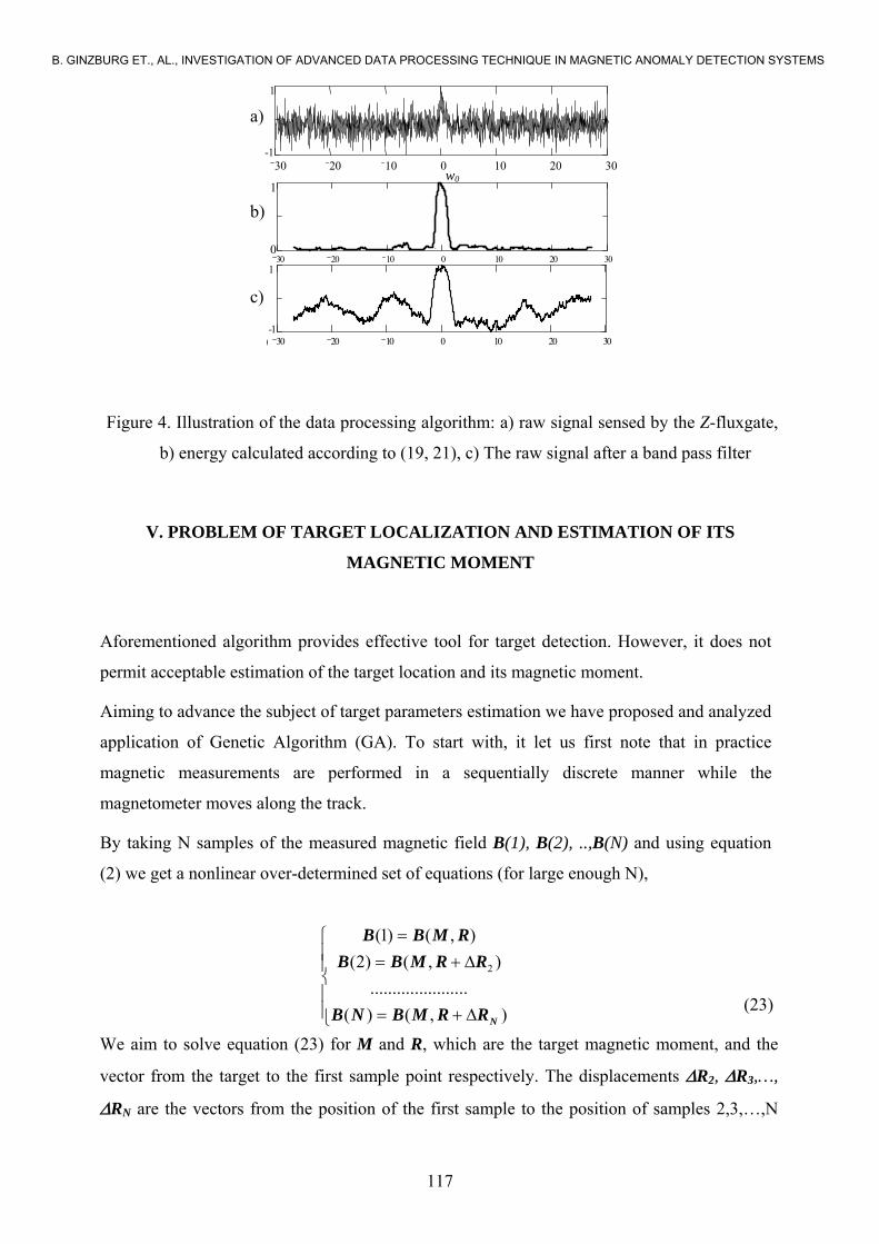
An example of application of given algorithm for target detection is shown in Fig. 4. Raw

data acquired by Z-fluxgate (Fig. 4a) contain bell-shaped dipole signal ( ,

, ) with SNR equal to 0.4. Data processing according to (19, 21) (Fig.

4b) increases SNR up to 12 which is much better than simple band-pass filtering (Fig 4c). It

is a consequence of the principle of algorithm (19 -22) which is based on prior guess of

magnetic dipole structure of the target signal.

27.0=xm

53.0=ym 80.0=zm

116


30 20 10 0 10 20 30

1

-1

w0

30 20 10 0 10 20 30

1

0 ( )

30 20 10 0 10 20 30

1

-1)

a)

b)

c)

Figure 4. Illustration of the data processing algorithm: a) raw signal sensed by the Z-fluxgate,

b) energy calculated according to (19, 21), c) The raw signal after a band pass filter

V. PROBLEM OF TARGET LOCALIZATION AND ESTIMATION OF ITS

MAGNETIC MOMENT

Aforementioned algorithm provides effective tool for target detection. However, it does not

permit acceptable estimation of the target location and its magnetic moment.

Aiming to advance the subject of target parameters estimation we have proposed and analyzed

application of Genetic Algorithm (GA). To start with, it let us first note that in practice

magnetic measurements are performed in a sequentially discrete manner while the

magnetometer moves along the track.

By taking N samples of the measured magnetic field B(1), B(2), ..,B(N) and using equation

(2) we get a nonlinear over-determined set of equations (for large enough N),

⎪⎪⎩

⎪⎨ ⎪⎧

Δ+=

Δ+==

),()(......................

),()2(),()1(

2

NRRMBNB

RRMBBRMBB

(23)

We aim to solve equation (23) for M and R, which are the target magnetic moment, and the

vector from the target to the first sample point respectively. The displacements ΔR2, ΔR3,…,

ΔRN are the vectors from the position of the first sample to the position of samples 2,3,…,N

117


respectively. These displacements can be measured precisely using advanced navigation

systems and therefore are considered as known. Solving equation (23) analytically is not trivial

especially in the presence of noise. That is why we have divided the problem domain is into

cells of predetermined resolution.

Each of the vectors M and R, consists of three Cartesian components, hence, one can define a

single six element solution vector, T

zyxzyx RRRMMM ),,,,,(== ),( RMX(24)

For each component of M and R there should be set a range according to practical

considerations concerning target possible location and magnetic dipole range. Then, for each

component of M and R there should be defined a resolution according to the needed accuracy.

A short example illustrates the process. Consider a search for a target, whose magnetic

moment ranges from -1 Am2 to+1 Am2. The needed accuracy for estimating the target

magnetic field is 0.02 Am2. Assume that the search takes place in a cube with a side length of

2 m, and we would like to localize target with accuracy of 2 cm. For each element of the

solution vector X, there are 100 possibilities, resulting in a finite solution space of a total 1006

possible solutions, from which we have to choose the nearest to actual one. As we see the

problem becomes that of searching the (sub) optimal solution out of a finite solution space

instead of solving equation (23) analytically. The limited range of possible solutions and the

restricted resolution result in sub optimal solutions rather than optimal, that is, however,

acceptable for many applications.

Checking all possible solutions one by one would consume enormous time, which is not

available in real time systems. For this reason we propose the Genetic Algorithm as a rapid

search method.

VI. APPLICATION OF GENETIC ALGORITHM FOR TARGET LOCALIZATION

AND ESTIMATION OF ITS MAGNETIC MOMENT

Genetic algorithms provide an effective way to solve problems such as traveling salesman (the

shortest route to visit a list of cities) [9]. In this work we focus on GA as a search method to

find the maximum of an object function, also called fitness function. The GA mimics the

evolutionary principle by employing three main operators: selection, crossover, and mutation.

118


As a first step we build a chromosome, which has the genotype of the desired solution. In the

case of localization of a magnetic dipole the chromosome has the form of (24). Each element

of the chromosome is called gene and may take only restricted values that were defined

previously by range and resolution as is explained in the former example. Implementing the

evolutionary principle obligates a collection of L chromosomes, which is entitled as

population. At first, random values are set for each chromosome of the population. A fitness

value is calculated for each chromosome by substituting for the chromosome into the fitness

function. The chromosomes can be arranged in a list from the fittest chromosome (with the

largest fitness result) to the least fit one. Then the selection operator is applied, selecting only

the K fittest chromosomes from the list. There are several ways to perform the selection,

which would not be described here. After selection, the crossover operator is utilized

resembling a natural breeding action. Only the K fittest chromosomes of the list are allowed to

breed amongst themselves by the following mathematical operation,

jinew XXX )1( λλ −+=(25)

Chromosomes Xi, Xj are randomly chosen from the list of the K fittest chromosomes. λ is a

crossover parameter (usually 0.5), and Xnew is a newborn chromosome. The process is

repeated until a population of K newborn chromosomes is reached. Afterward mutation

operator is implemented by randomly selecting a chromosome from the newborn population,

and changing a random gene to a random permitted value. The randomness property enables

the GA to overcome local minima. After mutation is applied, fitness evaluation is performed

on the mutated newborn population. The process of fitness evaluation-selection-crossover-

mutation is repeated for a predetermined number of generations or until the fittest

chromosome reaches a predefined fitness value. The convergence of the GA is expressed by

increase in the average fitness of the population from generation to generation. The

chromosome with the largest fitness value is chosen as the solution, according to ‘survival of

the fittest’ principle. Defining an appropriate fitness function is an important step in utilizing

GA. We have proposed the following fitness function for magnetic dipole localization by a 3-

axis magnetometer (without considering noise characteristics):

( ) ( )( )

∑=

−−X 2(Fitness (26) =

N

n

jj

nB

XBnB

1

2

)

119


where B(n) represents the n-th measurement sample while B(Xj) is the calculated magnetic

field produced by chromosome Xj. Note that the fittest chromosome fitness value is closest to

zero.

In order to investigate magnetic dipole localization by Genetic Algorithm, we performed

numerous computer simulations. To illustrate here some of simulation results we have chosen

magnetic dipole with Mx = 0.27 A⋅m2, My = 0.53 A⋅m2, Mz = 0.8 A⋅m2 located at the origin of

coordinate system (0,0,0). The samples were taken every 0.1 m from -7.1m to +7.1m along

the x-axis (south-north) at a constant y-axis coordinate of 6.7 m (see Fig. 1) and a constant

height of 2.4 m. so that a CPA distance R0 is of about 7 m. Random noise was added to the

magnetic dipole signal to ensure SNR value of 0.4 (Fig. 4a).The GA was set to a population of

100 chromosomes and a stop condition of 10,000 generations. The mutation probability was

set to 5% and the crossover probability to 30%. Statistical processing of the simulation results

after 100 executions leads to the following results.

a. Moment estimation

Total magnetic moment of the target dipole is 1 A⋅m2. Estimated magnetic moment averaged

over 100 executions of GA algorithm was 1.1 A⋅m2 – relative biased estimate value of 10%.

Statistical distribution of the obtained moment values is shown in Fig. 5.

Figure 5. Distribution of magnetic moments obtained as a result of 100 GA executions.

b. Target localization

Estimated target location averaged over 100 executions of GA algorithm was (-0.26m, -

0.45m, 0.07m) so that absolute biased estimate length was 0.53m which makes up less than

120


10% error relative to CPA distance. Spatial distribution of the obtained target locations is

shown in Fig. 6.

Track of the sensors platform

Figure 6. Spatial distribution of target locations obtained as a result of 100 GA executions.

VII. CONCLUSION

In the present work we have investigated two approaches to the data processing of the MAD

signals.

Our first approach to MAD signal processing relies on the decomposition of the MAD signal

in the space of specially constructed orthonormalized functions. It turns out the signals of

fluxgate sensor type can be presented as a linear combination of three orthonormal functions

while the search coil signals need four orthonormal functions for correct representation. The

dipole energy signal is introduced in the basis chosen and is found to be a useful function for

the data processing algorithm based upon the results of the modeling. It is important to

underline this method works equally well for various orientations of target moment relative

to external Earth’s magnetic field and direction of survey line. The aforementioned

processing procedure provides a considerable improvement of the SNR thus enabling reliable

target detection even with low values of SNR.

To proceed with target parameters estimation we proposed and tested another approach to

MAD signal processing based on Genetic Algorithm. Typical parameters of GA included:

population of 100 chromosomes; stop condition of 10,000 generations; mutation probability

5%; crossover probability 30%. Statistical processing of the simulation results after 100

executions shows good algorithm convergence and acceptable (<10%) relative errors of main

target parameters estimation even with rather low signal-to-noise ratio in raw magnetometer

121


signal. Further investigation addresses a comparison of the GA to other global optimization

methods such as the simulated annealing (SA) for magnetic target localization and magnetic

moment estimation [10].

REFERENCES

[1] M. Hirota, T. Furuse, K. Ebana, H. Kubo, K. Tsushima, T. Inaba, A. Shima, M. Fujinuma

and N. Tojyo, “Magnetic detection of a surface ship by an airborne LTS SQUID MAD”,

IEEE Trans. Appl. Supercond. 11 (2001) 884-887.

[2] W.M. Winn, in: C. E. Baum (Ed.), Detection and Identification of Visually Obscured

Targets, Taylor and Francis, Philadelphia, PA, 1999, Chapter 11, 337-376.

[3] H. Zafrir, N. Salomonski, Y. Bregman, B. Ginzburg, Z. Zalevsky, M. Baram, “Marine

magnetic system for high resolution and real time detection and mapping of ferrous

submerged UXO, sunken vessels, and aircraft”, in: Proc. UXO/Countermine Forum 2001,

New Orleans, LA, 9-12 April 2001.

[4] R. B .Semevsky, V. V. Averkiev, V. V. Yarotsky, Special Magnetometry, 2002, “Nauka”,

pp.228, St.-Petersburg, (in Russian)

[5] G.A. Korn and T.M. Korn, Mathematical Handbook for Scientists and Engineers,

McGraw Hill, New York, second ed., 1968, p. 491.

[6] Y. D. Dolinsky, “Vliyanie osobennostei signala na strukturu optimalnogo priemnika pri

obnaruzhenii namagnichennykh tel”, Geofizicheskaya Apparatura, 97 (1993) 29-38 (in

Russian).

[7] B. Ginzburg, L. Frumkis and B.Z. Kaplan, “Processing of magnetic scalar magnetometer

signals using orthonormal functions”, Sens. Actuators A 102 (2002) 67-75.

[8] H. C. Seran , P. Fergeau, "An optimized low-frequency three-axis search coil

magnetometer for space research", Review of Sci. Instr., 76, pp 044502-1 – 044502-10

(2005).

[9] F. O. Karray, C. DeSilva Soft Computing and Intelligent Systems Design Theory, Tools

and Applications, Addison Wesley, England, (2004).

[10] A. Sheinker, B. Lerner, N. Salomonski, B. Ginzburg, L. Frumkis and B.-Z. Kaplan,

“Localization and magnetic moment estimation of a ferromagnetic target by simulated

annealing”, Measurement Science and Technology, Vol. 18, pp 3451-3457, (2007).

122


http://www.iop.org/EJ/search_author?query2=Arie%20Sheinker&searchfield2=authors&journaltype=all&datetype=all&sort=date_cover&submit=1

http://www.iop.org/EJ/search_author?query2=Boaz%20Lerner&searchfield2=authors&journaltype=all&datetype=all&sort=date_cover&submit=1

http://www.iop.org/EJ/search_author?query2=Nizan%20Salomonski&searchfield2=authors&journaltype=all&datetype=all&sort=date_cover&submit=1

http://www.iop.org/EJ/search_author?query2=Boris%20Ginzburg&searchfield2=authors&journaltype=all&datetype=all&sort=date_cover&submit=1

http://www.iop.org/EJ/search_author?query2=Lev%20Frumkis&searchfield2=authors&journaltype=all&datetype=all&sort=date_cover&submit=1

http://www.iop.org/EJ/search_author?query2=Ben%2dZion%20Kaplan&searchfield2=authors&journaltype=all&datetype=all&sort=date_cover&submit=1

Date post:	12-May-2018
Category:	Documents
Upload:	vodang
View:	215 times
Download:	1 times

Investigation of advanced data processing technique in...

Documents