Thermogravimetric technique for volatiles detection...

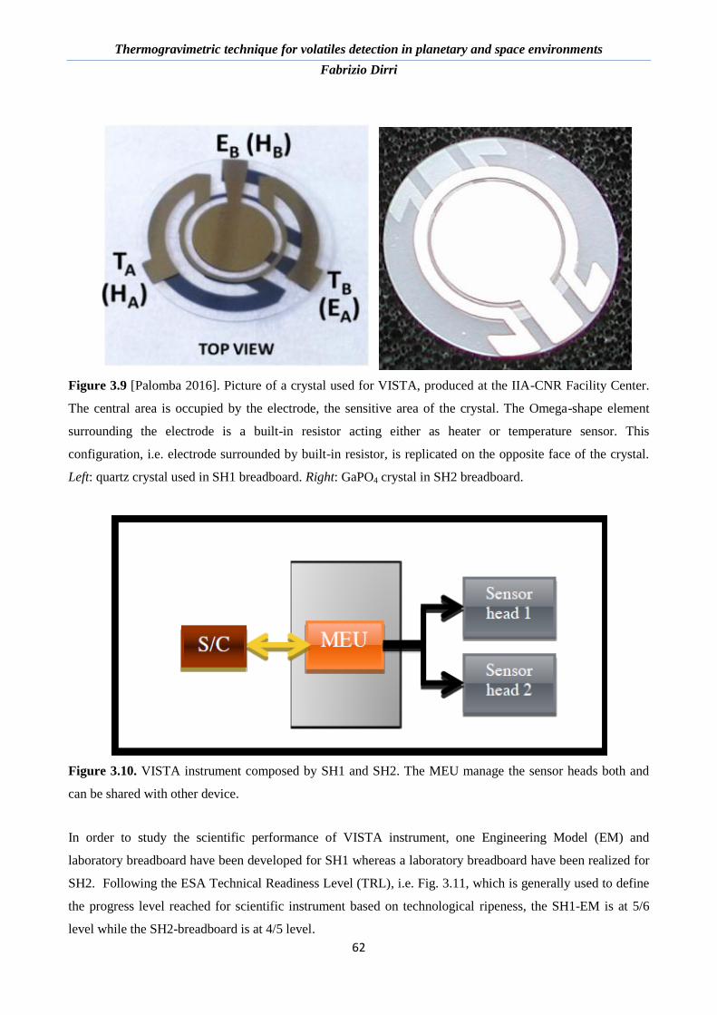
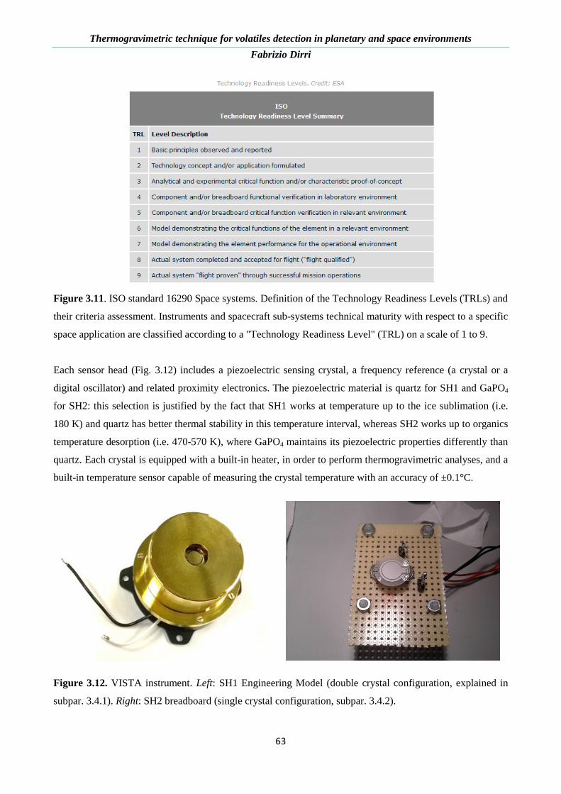
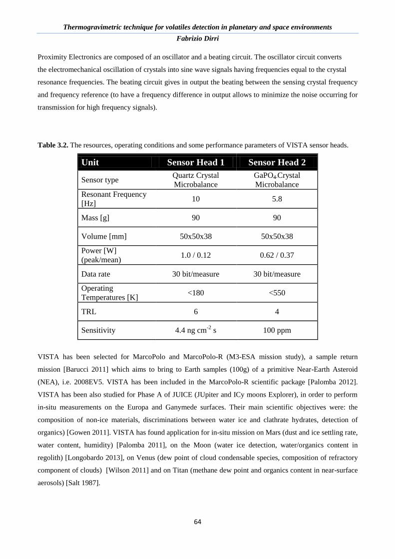
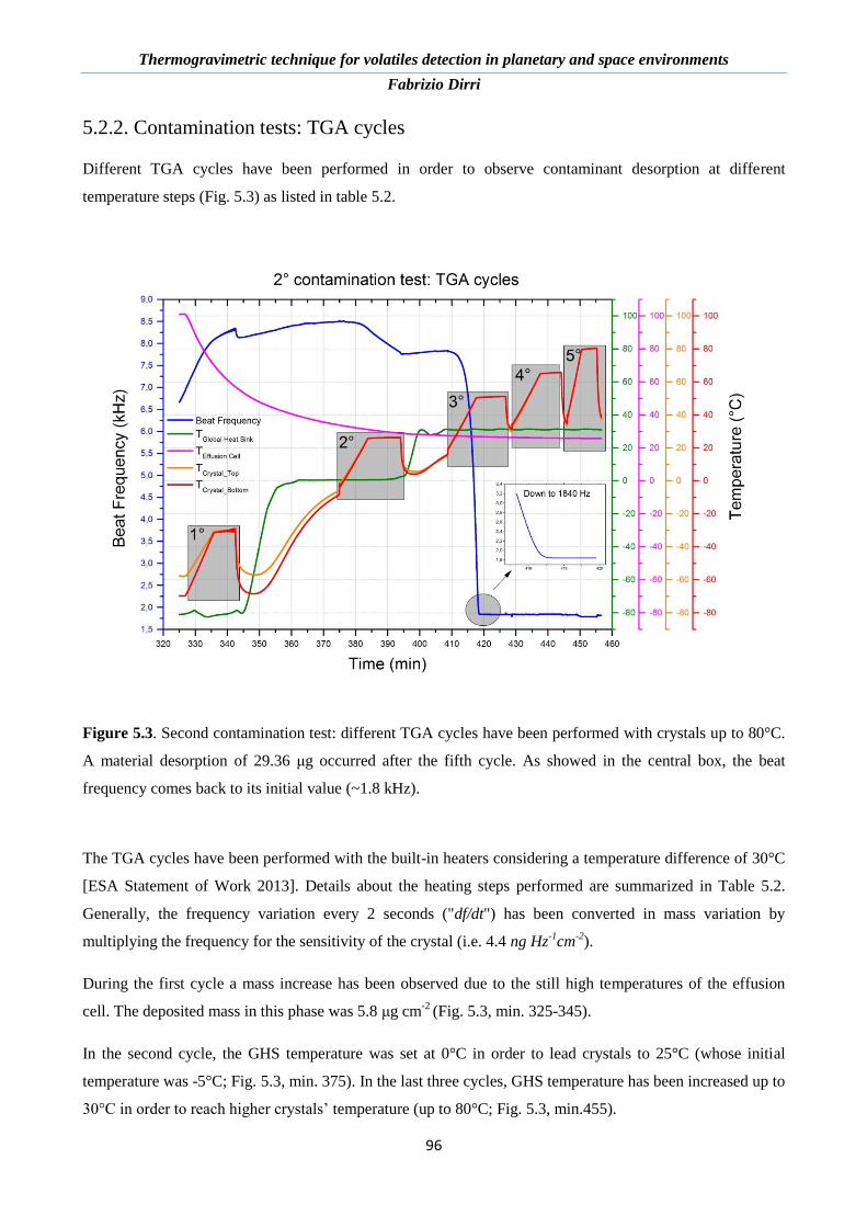
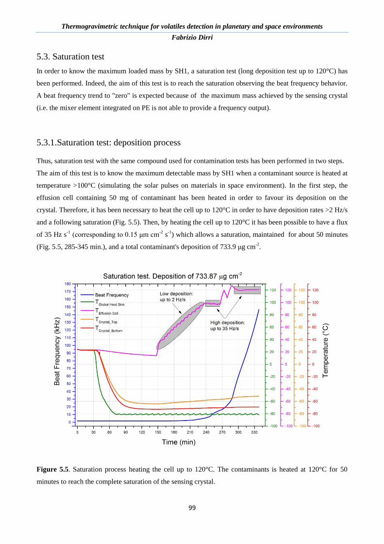
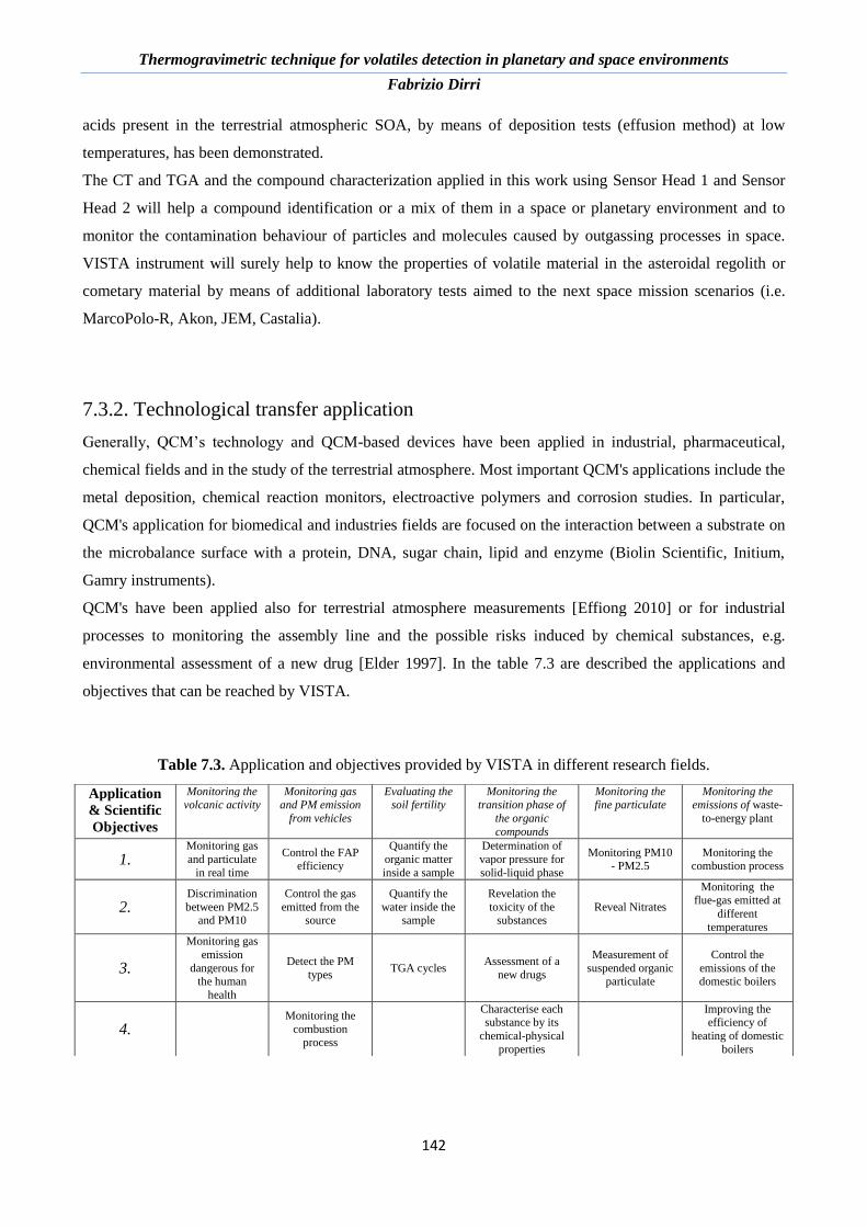
SAPIENZA UNIVERSITÁ DI ROMA

Ph.D. in Information and Communication Technologies

Curriculum: Radar and Remote Sensing

Cycle XXIX

_____________________________________________________

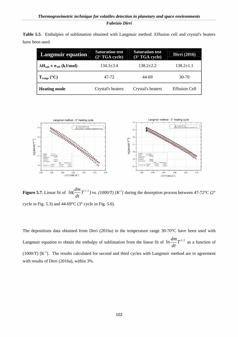
Ph.D. Dissertation

THERMOGRAVIMETRIC TECHNIQUE FOR

VOLATILES DETECTION IN PLANETARY AND

SPACE ENVIRONMENTS

Candidate Tutor

Fabrizio Dirri Prof. Frank Silvio Marzano

Dr. Ernesto Palomba

Academic Year 2015-2016

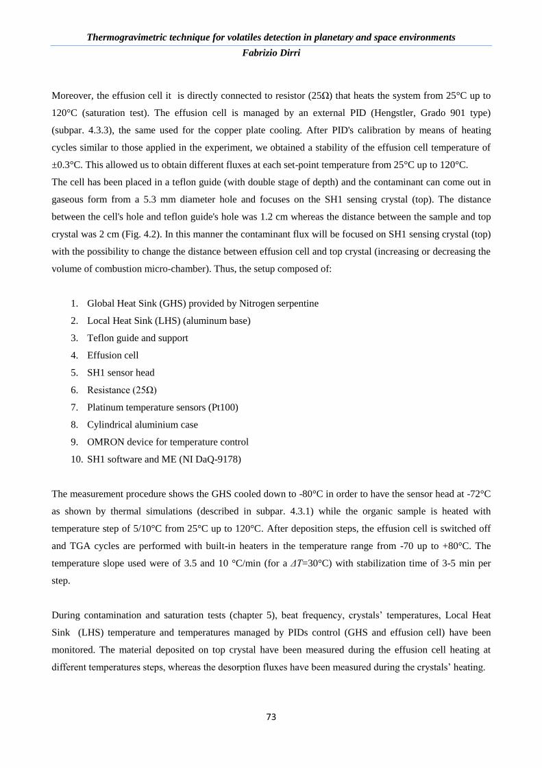
Thermogravimetric technique for volatiles detection in planetary and space environments

Fabrizio Dirri

2


Fabrizio Dirri

3

Abstract Introduction. The PhD work has been performed at Institute of Astrophysics and Space Planetology (IAPS-

INAF) in the framework of the two projects VISTA (Volatile In-Situ Thermogravimeter Analyser) and CAM

(Contamination Assessment Microbalance), funded by Italian Space Agency and European Space Agency,

respectively, both aiming at developing a microbalance sensor for space mission applications, i.e. to study

the minor bodies of Solar System (i.e., ESA-M5 Missions Call, MarcoPolo-M5, Akon, JEM and Castalia) by

measuring in-situ volatiles material of scientific interest (VISTA project) and to assess the contamination

issue (CAM project).

VISTA is a miniaturized thermogravimeter (composed by Piezoelectric Crystal Microbalance and the related

Proximity Electronics), based on Thermogravimetric Analysis (TGA), i.e. a widely used technique to

monitor the processes involving compounds, i.e. absorption/desorption and evaporation/sublimation. Thanks

to the variation in the microbalance oscillation frequency it is possible to estimate the sample mass

loss/deposited from thermal cycles. VISTA is composed of two sensor heads, i.e. the Sensor Head 1 (SH1)

for in-orbit contamination measurements from outgassing processes and Sensor Head 2 (SH2) for planetary

in-situ measurements, respectively. The breadboard and the Engineering Model of VISTA SH1 have been

developed for ESA Project, i.e. CAM, an Invitation to Tender of European Space Agency (EMITS-ESA)

aiming at developing a thermogravimeter for contamination measurements in space, leaded by IAPS-INAF

and developed by a consortium of three Italian institutes and one Industry. The VISTA SH2 breadboard has

been developed in the framework of MarcoPolo-R Mission, where VISTA was part of the scientific payload.

Objectives. In this work, the VISTA capability to monitor the contamination processes in space environment

and for the study of planetary surfaces and atmospheres has been demonstrated as well as the good capability

of sensor heads to monitoring and to characterizing a contaminant source and organic compounds by

realizing TGA cycles and Effusion Method (EM) to obtain the vapor pressures and enthalpy of sublimation.

Material and Method. The first phase of the work was based on the study of Volatile Organic Compounds

(VOCs): 1) in planetary atmospheres including their physical-chemical properties and their connections with

the atmospheric aerosol sources (biogenic and anthropogenic); 2) in space, coming from outgassing

processes of materials exposed to space environment, and the related instrumentation issues. Thus, organic

compounds (found in Carbonaceous Chondrite meteorites and in Earth's VOCs) have been selected to

perform deposition processes and TGA cycles obtaining a complete characterization with SH1 and SH2. The

vapor pressures and enthalpy of sublimation were identified as those thermochemical parameters able to

characterize a kinetics process regarding VOCs in planetary atmosphere and in space. Thus, a laboratory

activity was planned and divided in a first design and development phase of two laboratory setup and in a

second calibration phase of VISTA sensor heads. A third phase was devoted at performing different tests for

contamination study in space (using a contaminant source and SH1 breadboard) and for VOCs

characterization in atmosphere (using five dicarboxylic acids and SH2 breadboard). Results. The breadboards

of VISTA instrument SH1 and SH2 have been developed to monitor the contamination in space (SH1) and to

characterize organic compounds (SH2). The main results reached in the PhD work with VISTA SH1 have

been: 1) to monitor contamination processes in vacuum chamber simulating the space environment (between

5x10-9

to 7x10-4

g/cm2); 2) the contaminant source characterization by means of TGA cycles (ΔTmax~60°C)

and retrieval of vapour pressure of compounds (Pi) and the enthalpy of sublimation (ΔHsub) by using the

Langmuir and Clausius-Clapeyron relations; 3) the sensor regeneration by means of thermal cycles by using

the integrated heaters on crystal surface (with an accuracy within 0.1°C). On the other hand, the main

scientific objectives reached with VISTA SH2 have been: 1) the volatiles material measurement deposited on

the sensor surface at different temperatures by using the Effusion Method simulating the asteroidal/cometary

environment; 2) the characterization of VOCs, i.e. dicarboxylic acids, by calculating the enthalpy of

sublimation (ΔHsub) with Van't Hoff relation. Conclusion. In this work, the VISTA SH1 and SH2

Breadboards have been designed and developed as well as two different laboratory set-up to verify the

capability of SH1 and SH2 to monitor a contamination process and to characterize a pure organic compound,

respectively, using TGA cycles and EM. The enthalpies of sublimation results obtained with SH1 from one

contaminant source (adipic acid) using TGA and EM, are in agreement within 3.5% while the enthalpies of

sublimation obtained for five dicarboxylic acids and using EM, are in agreement within 6% (oxalic, succinic

and adipic acids) and 11% (azelaic and suberic acids) with previous works. These results demonstrate the

capability of SH1 and SH2 Breadboards to detect organic contaminant and to characterize different organic

compounds presents in VOCs terrestrial atmosphere obtaining a good characterization for a pure compound.


Fabrizio Dirri

4


Fabrizio Dirri

5

Index

Abstract ............................................................................................................................................................ 3

Acronym List ................................................................................................................................................... 9

Chapter 1. Introduction ................................................................................................................................ 12

Chapter 2. VOCs in terrestrial atmosphere and space .............................................................................. 17

2.1 Introduction ........................................................................................................................................... 17

2.2. Terrestrial atmospheric aerosols ........................................................................................................... 17

2.2.1. VOC and SOA ............................................................................................................................... 20

2.2.2. Organic fraction of VOC and SOA ............................................................................................... 21

2.2.3. Marker substances in SOA ............................................................................................................ 22

2.2.4. Continental and background aerosols monitoring ......................................................................... 23

2.3. VOC detection in space ........................................................................................................................ 25

2.3.1. Outgassing process and instrument issues ..................................................................................... 26

2.3.2. Contamination measurement on ISS, Mir, STS and Satellites ...................................................... 29

2.4. Volatiles reservoirs in planetary bodies detectable by TGA ................................................................ 34

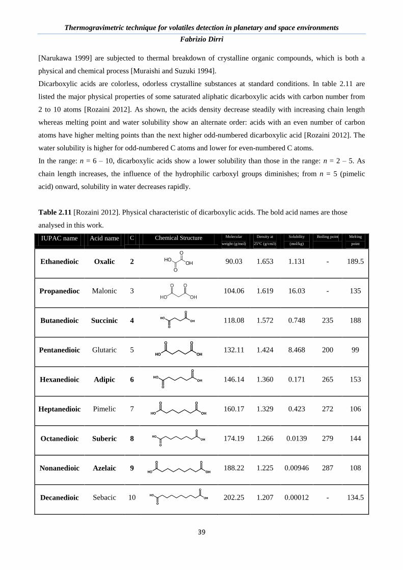
2.5. Dicarboxylic acids ................................................................................................................................ 37

2.5.1. Physical properties ......................................................................................................................... 38

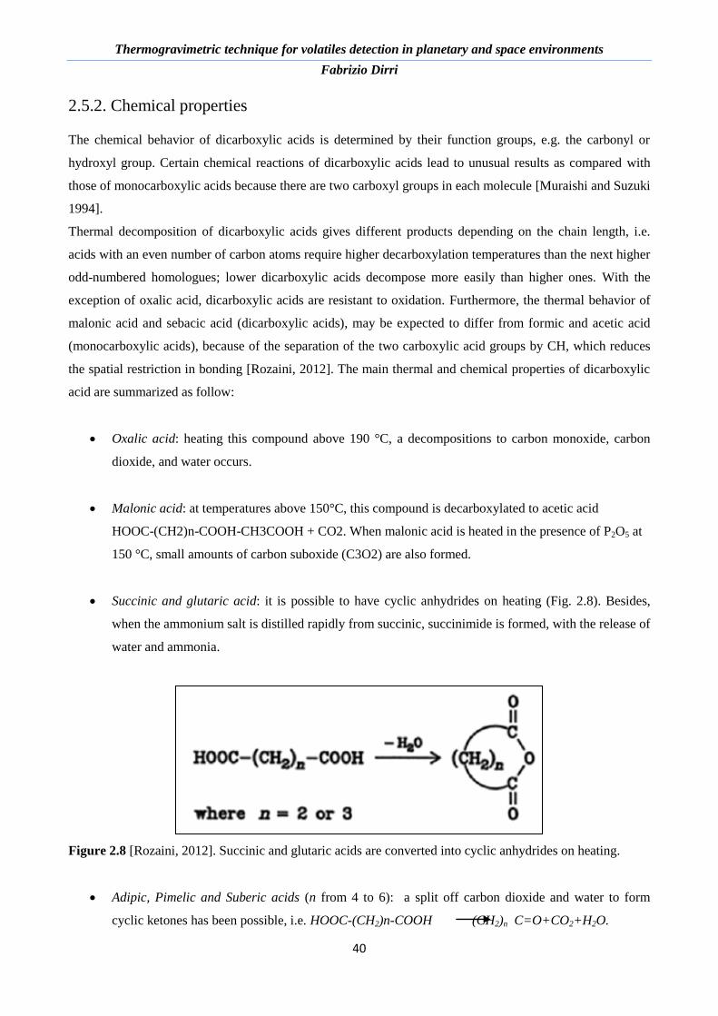
2.5.2. Chemical properties ....................................................................................................................... 40

2.5.3. Bio-markers compounds ................................................................................................................ 41

Chapter 3. Thermo-physics and Thermogravimetry: basic concept ........................................................ 44

3.1. Introduction .......................................................................................................................................... 44

3.2. Thermochemical processes ................................................................................................................... 44

3.2.1. Phase change thermodynamic processes ....................................................................................... 44

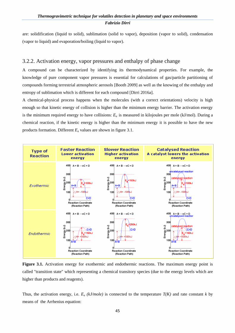
3.2.2. Activation energy, vapor pressures and enthalpy of phase change ............................................... 45

3.2.3. Entropy and Gibbs free energy: spontaneous and non-spontaneous reactions ............................. 49

3.2.4. Enthalpy and Entropy of sublimation from Gibbs free energy ..................................................... 51

3.3. Thermogravimetry: basic concept ........................................................................................................ 52

3.3.1. Introduction to transduction mass sensors ..................................................................................... 54

3.3.2. Microbalance working principle .................................................................................................... 54

3.3.3. QCM and TGA application ........................................................................................................... 60

3.4. VISTA instrument ................................................................................................................................ 61

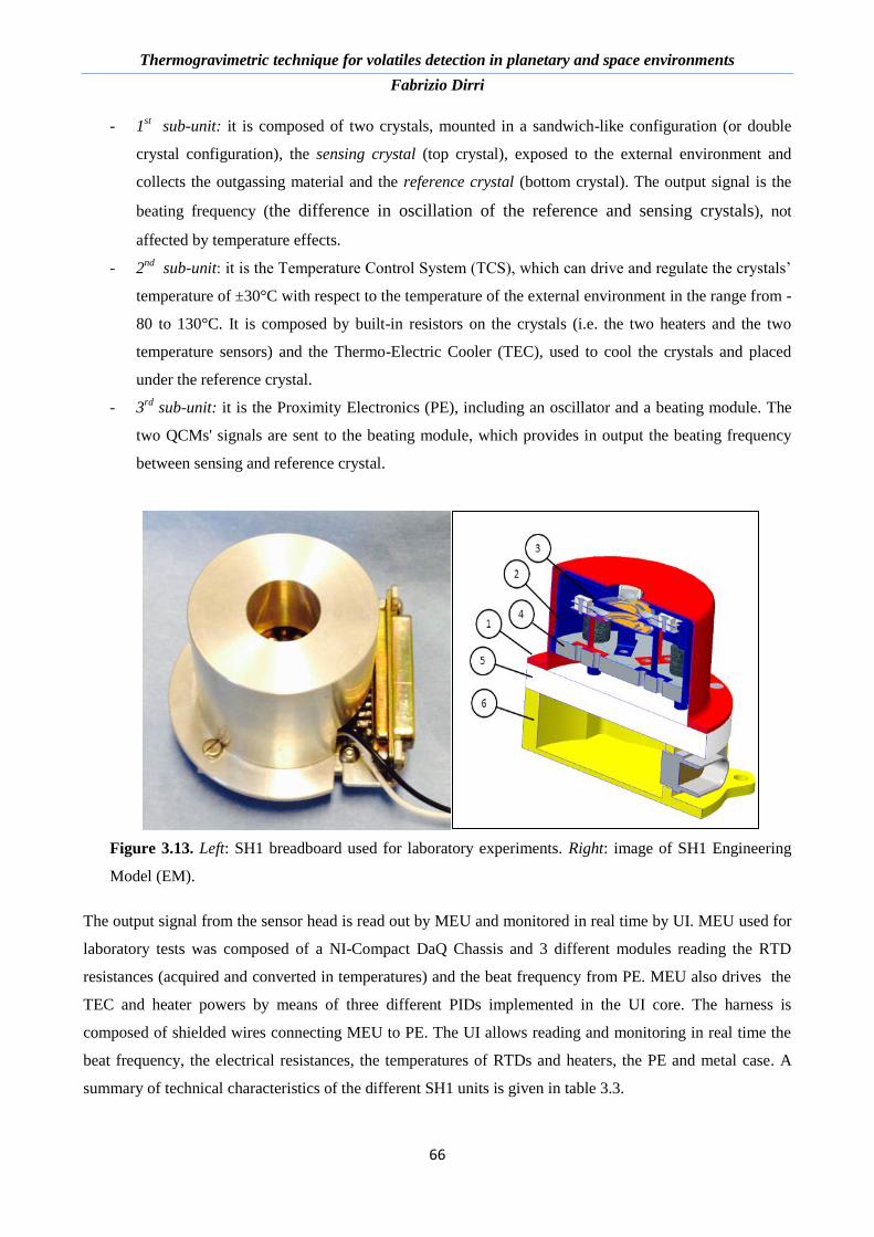
3.4.1. VISTA Sensor Head 1 for VOCs monitoring in space .................................................................. 65

3.4.2. VISTA Sensor Head 2 for atmospheric VOCs characterization ................................................... 67

3.4.3. Aim of the work ............................................................................................................................. 68

Chapter 4. Laboratory set-up development ................................................................................................ 70

4.1. Introduction .......................................................................................................................................... 70


Fabrizio Dirri

6

4.2. Monitored processes and method ......................................................................................................... 70

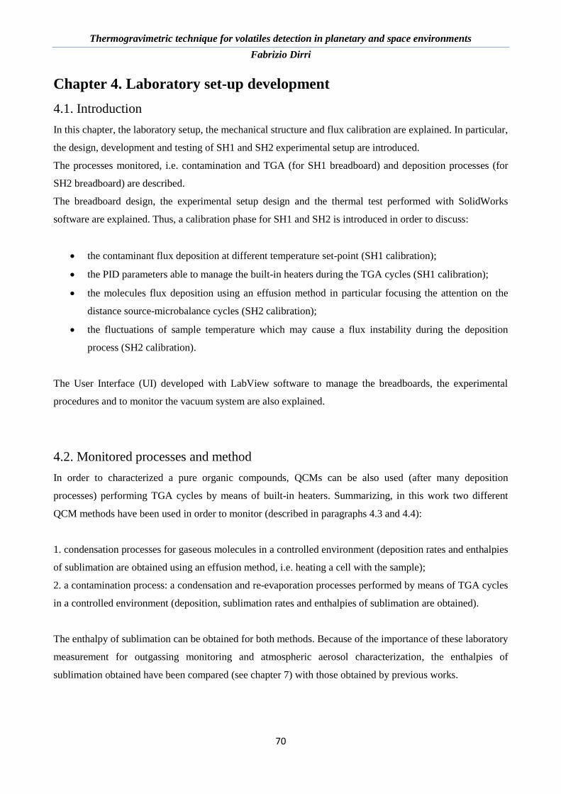
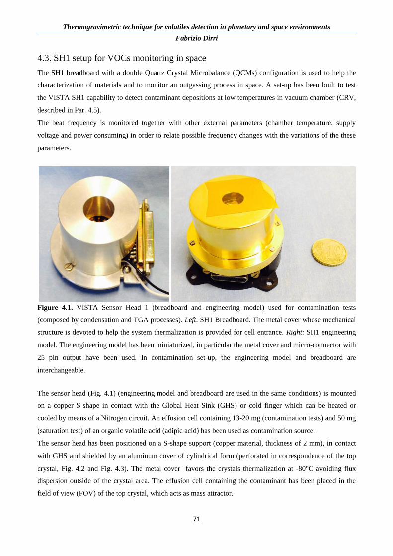
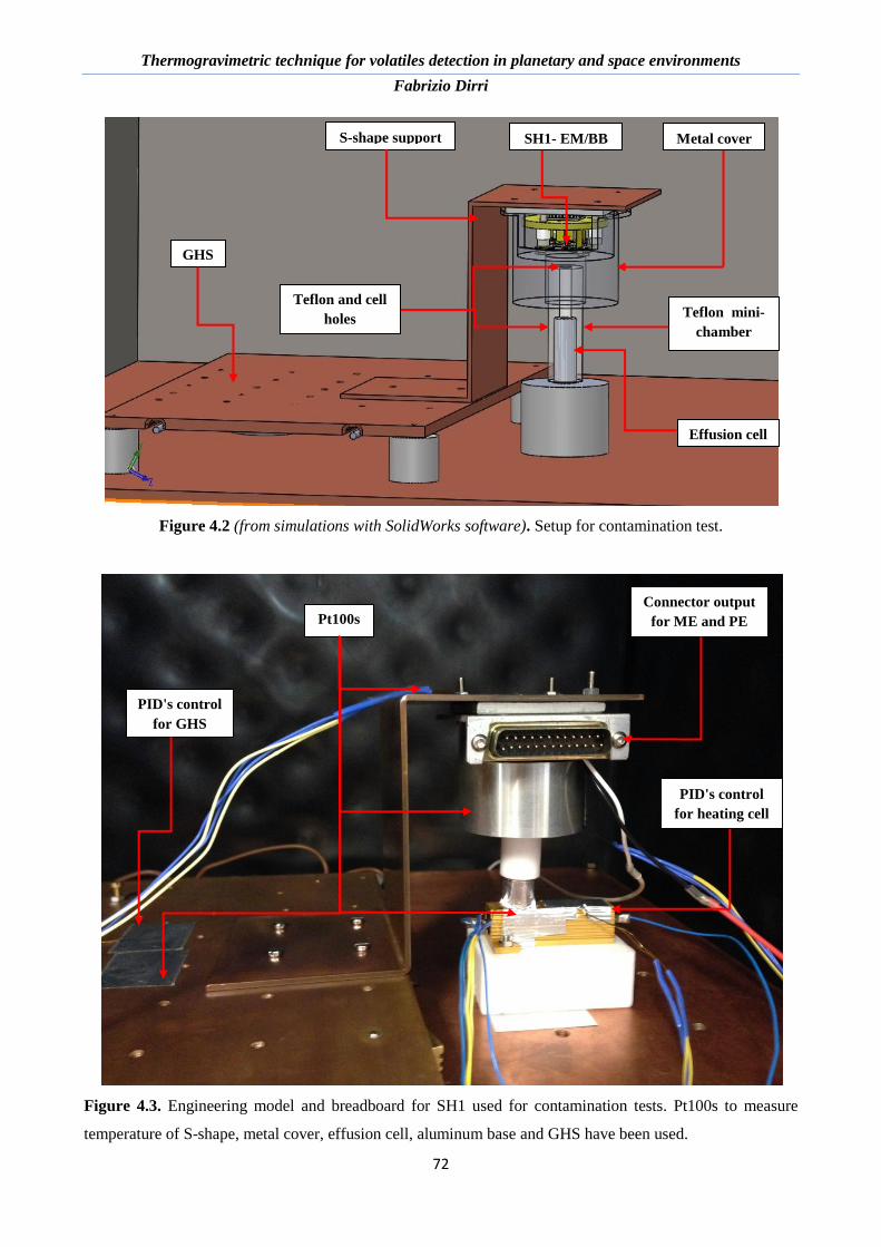
4.3. SH1 setup for VOCs monitoring in space ............................................................................................ 71

4.3.1 Thermal simulations ....................................................................................................................... 74

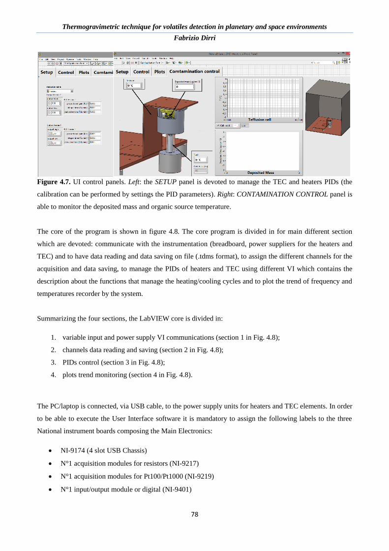
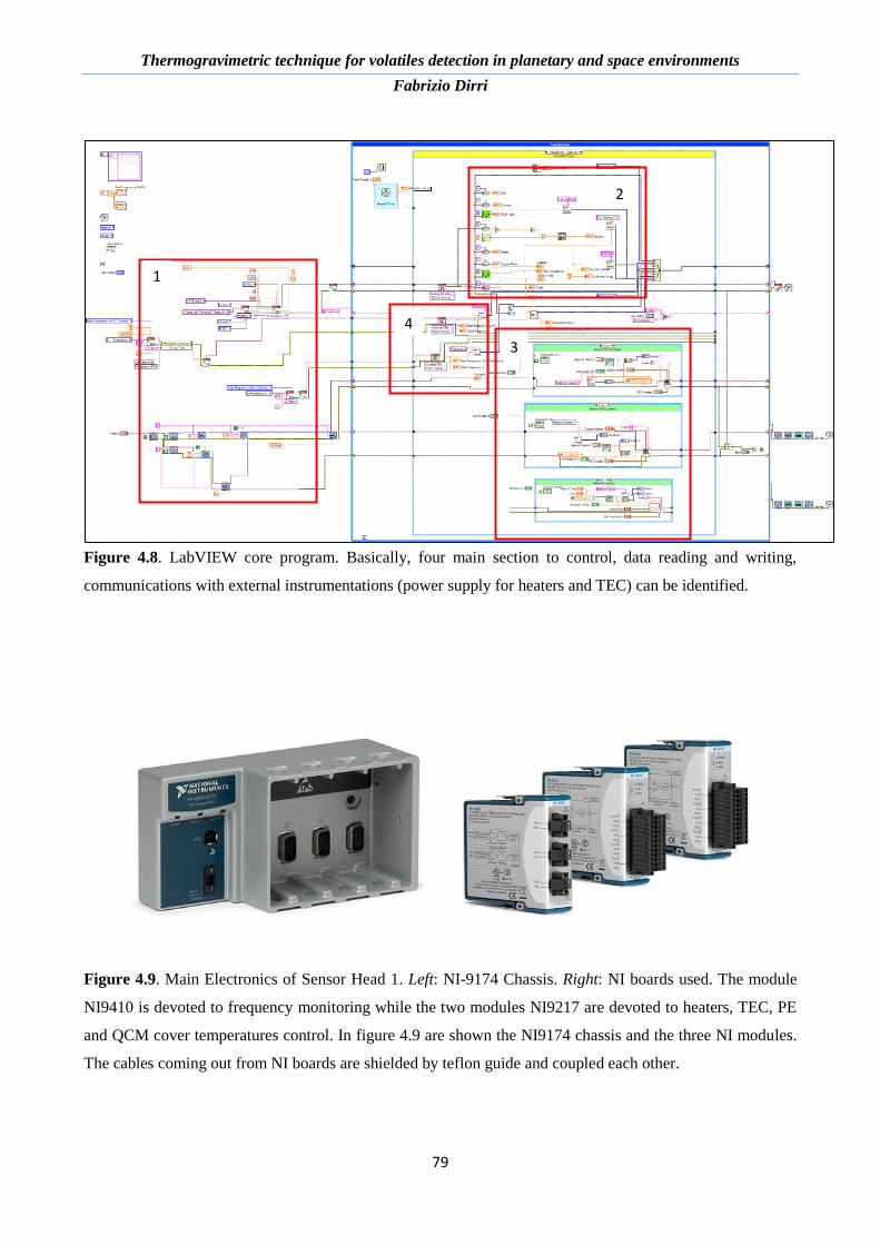
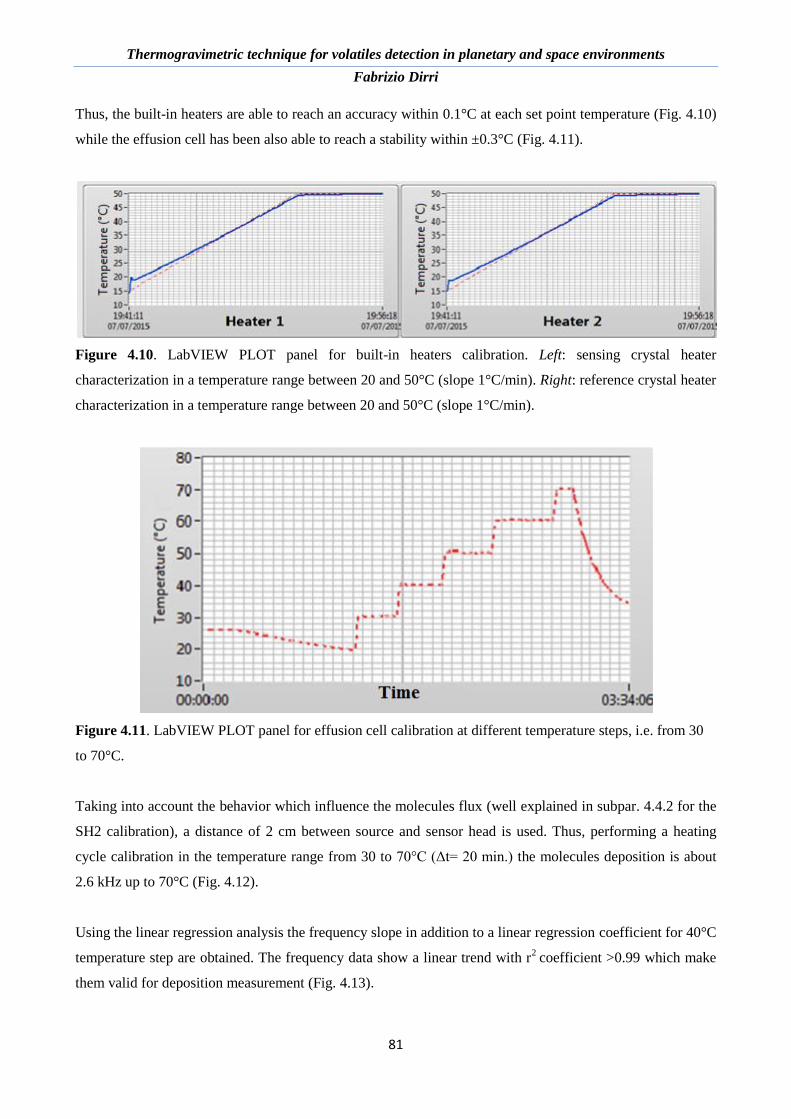
4.3.2. User Interface and Main Electronics ............................................................................................. 77

4.3.3. PIDs parameters and flux calibration ............................................................................................ 80

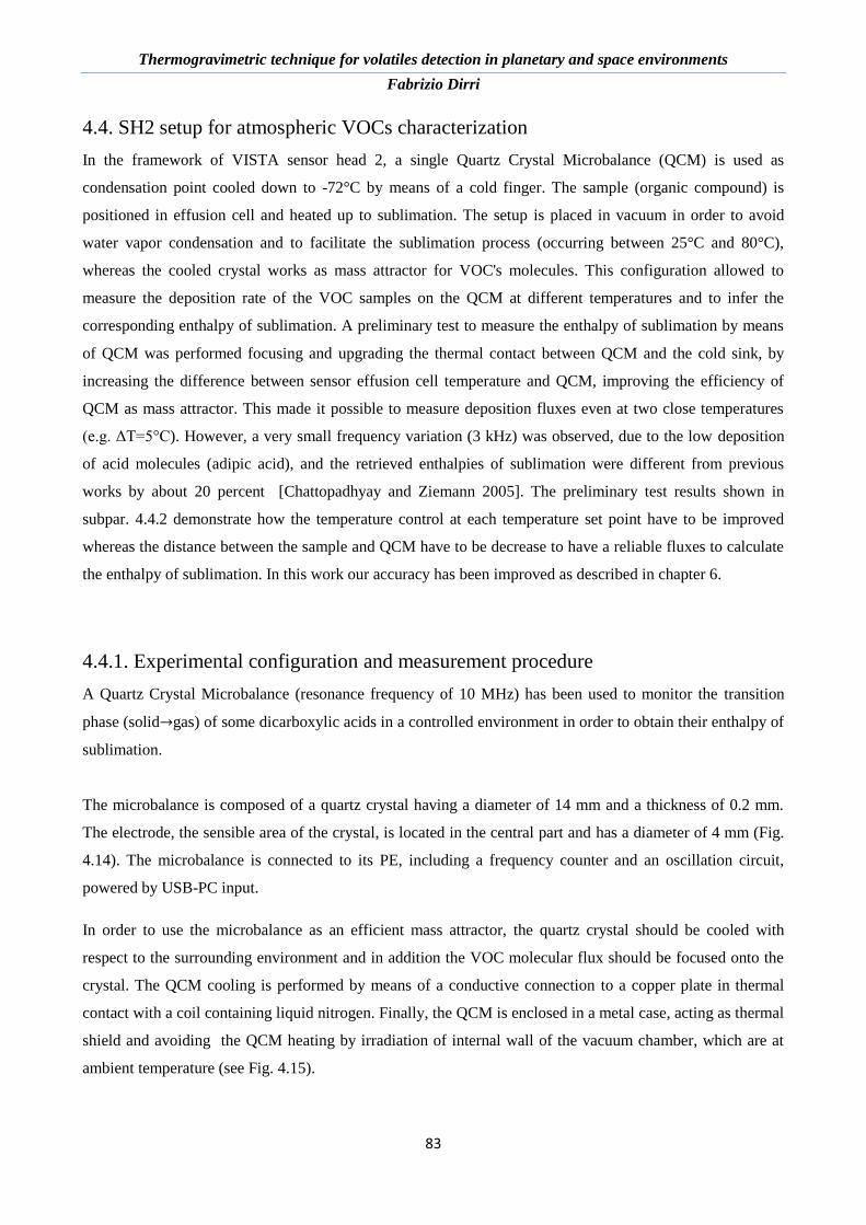
4.4. SH2 setup for atmospheric VOCs characterization .............................................................................. 83

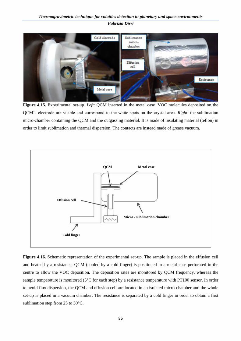
4.4.1. Experimental configuration and measurement procedure ............................................................. 83

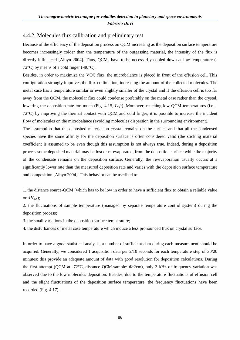
4.4.2. Molecules flux calibration and preliminary test ............................................................................ 86

4.5. Vacuum system and data acquisition system........................................................................................ 88

4.6. Setup and measurement procedures summary ...................................................................................... 89

Chapter 5. SH1 for contamination monitoring in space ............................................................................ 92

5.1. Introduction .......................................................................................................................................... 92

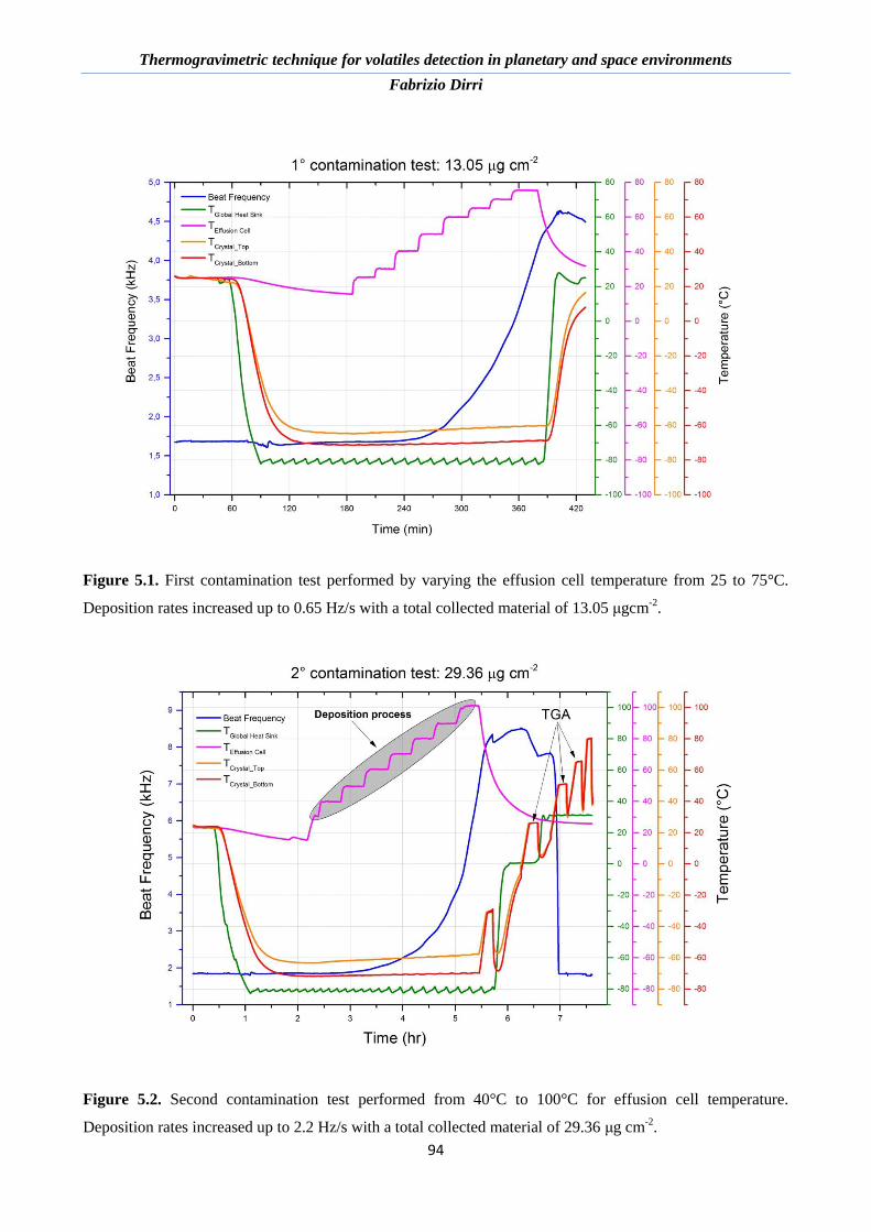
5.2. Contamination tests .............................................................................................................................. 93

5.2.1. Contamination tests: deposition processes .................................................................................... 93

5.2.2. Contamination tests: TGA cycles .................................................................................................. 96

5.3. Saturation test ....................................................................................................................................... 99

5.3.1.Saturation test: deposition process.................................................................................................. 99

5.3.2. Saturation test: TGA cycles ......................................................................................................... 100

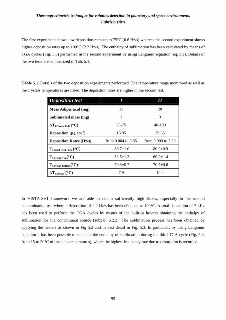
5.4. Enthalpy of sublimation results comparison ...................................................................................... 103

Chapter 6. Atmospheric VOCs characterization: results ........................................................................ 105

6.1. Introduction ........................................................................................................................................ 105

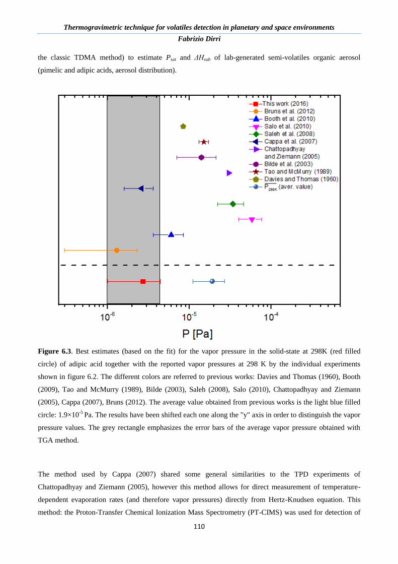
6.2. SH1 for organic compound characterization (TGA method) ............................................................. 106

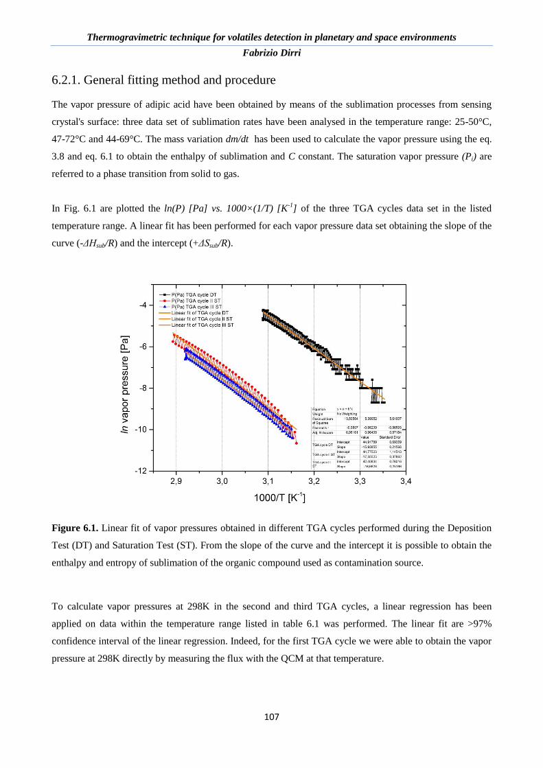
6.2.1. General fitting method and procedure ......................................................................................... 107

6.2.2. Pi and ΔHsub : results and comparison ........................................................................................ 108

6.3. SH2 for organic compounds characterization (Effusion Method) ...................................................... 112

6.4. Experimental activity .......................................................................................................................... 113

6.4.1. Measurement procedure and data acquisition method ................................................................. 113

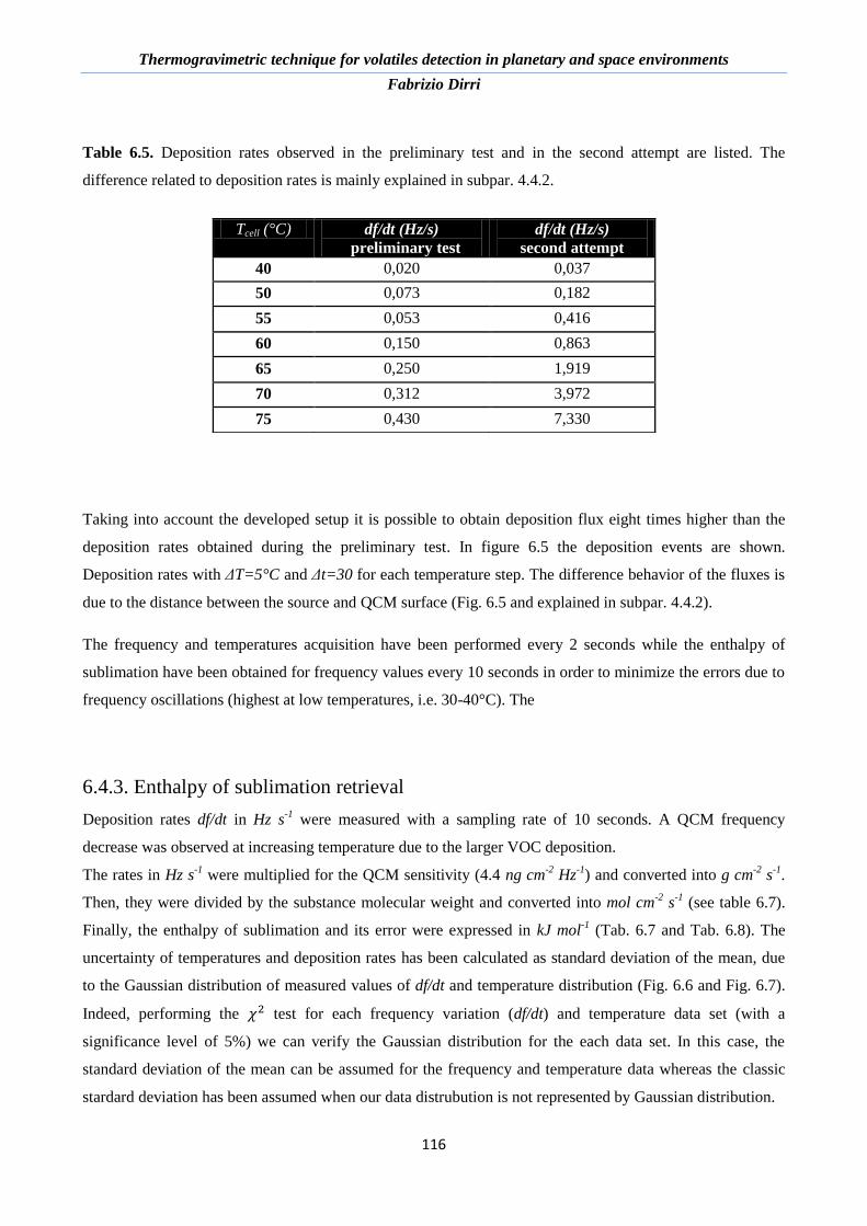
6.4.2. Deposition rates ........................................................................................................................... 115

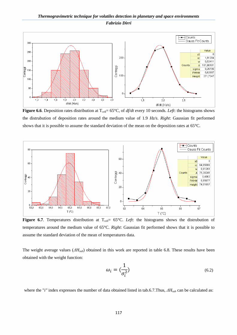
6.4.3. Enthalpy of sublimation retrieval ................................................................................................ 116

6.5. Data analysis and results..................................................................................................................... 118

6.5.1. Oxalic acid (C2) ........................................................................................................................... 118

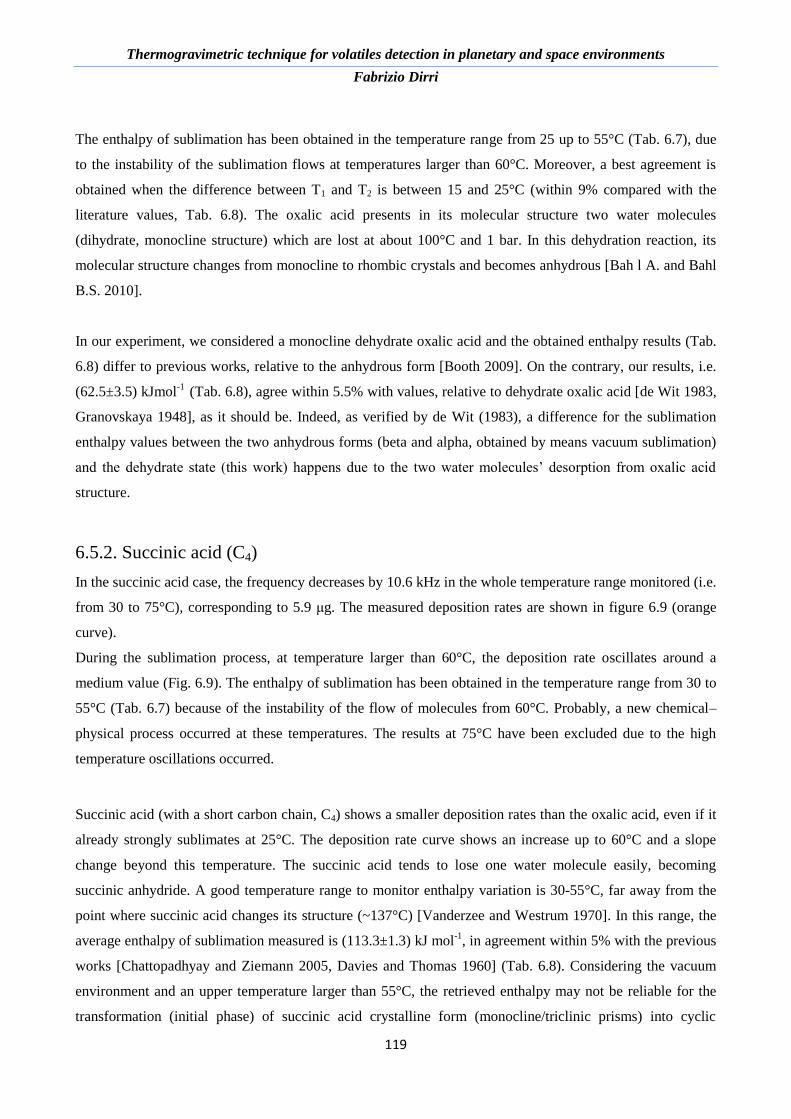
6.5.2. Succinic acid (C4) ........................................................................................................................ 119

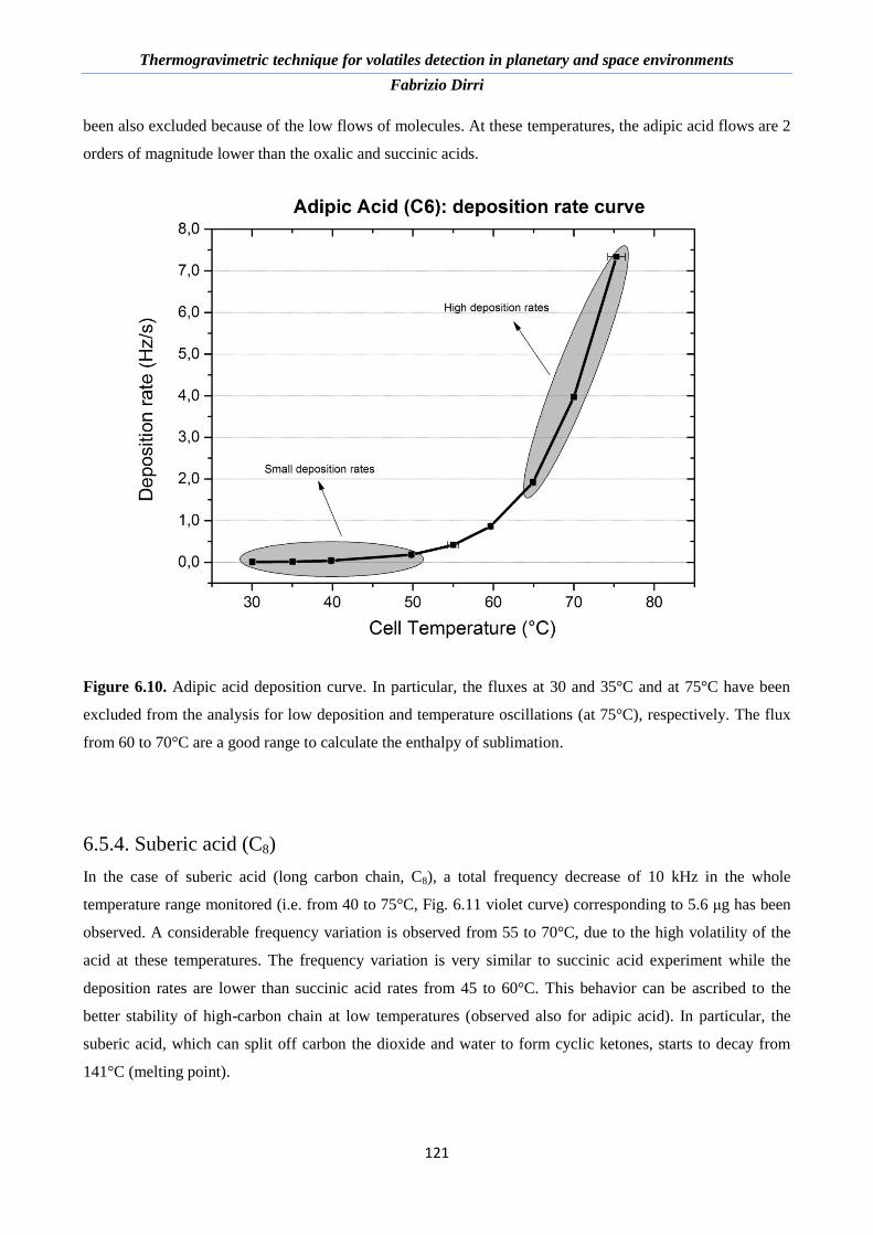
6.5.3. Adipic acid (C6) ........................................................................................................................... 120

6.5.4. Suberic acid (C8) .......................................................................................................................... 121

6.5.5. Azelaic acid (C9) .......................................................................................................................... 122

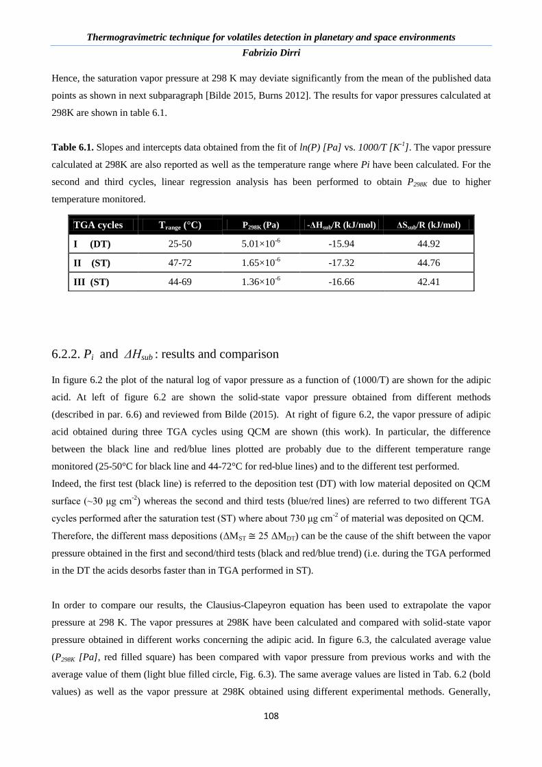
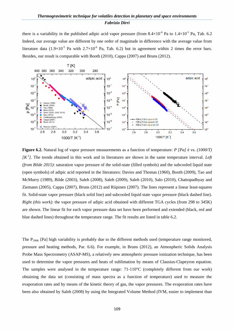
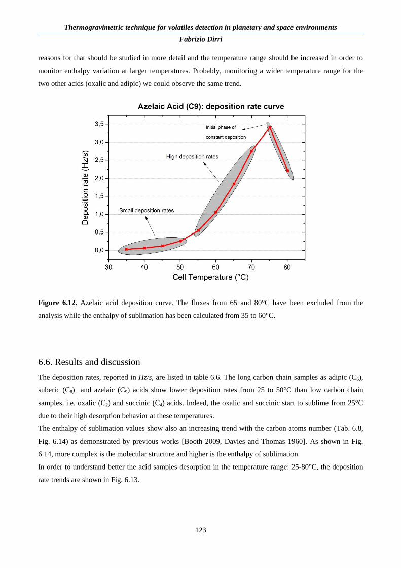
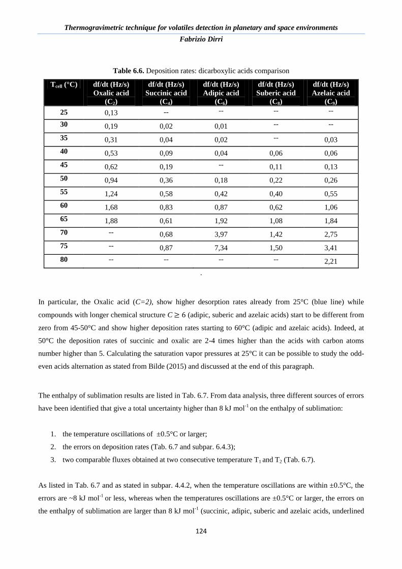
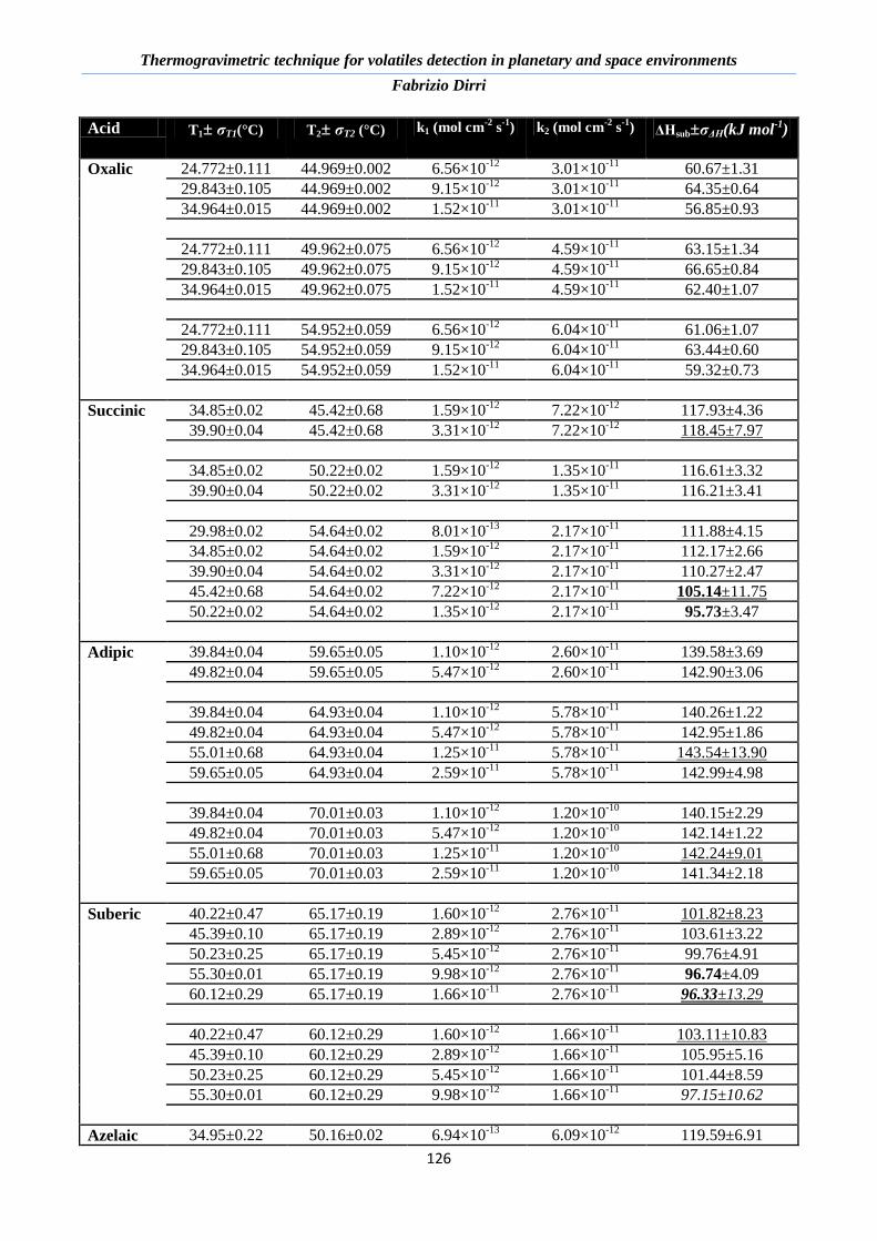
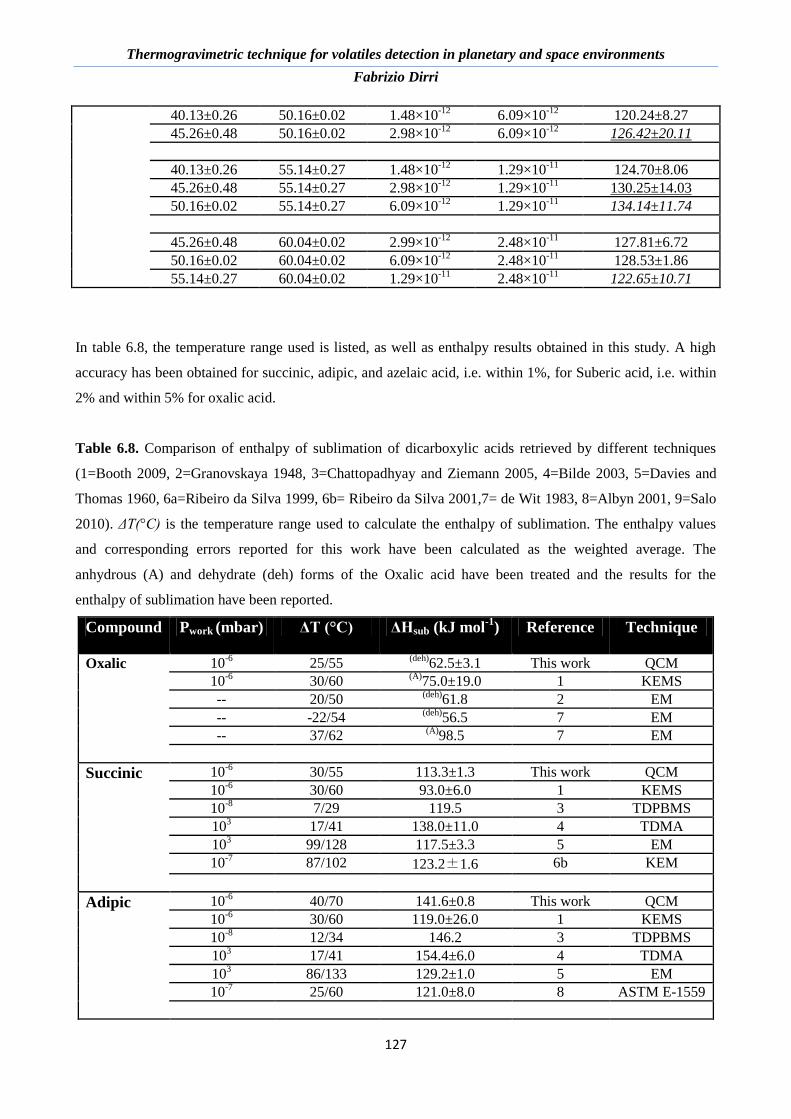
6.6. Results and discussion ........................................................................................................................ 123


Fabrizio Dirri

7

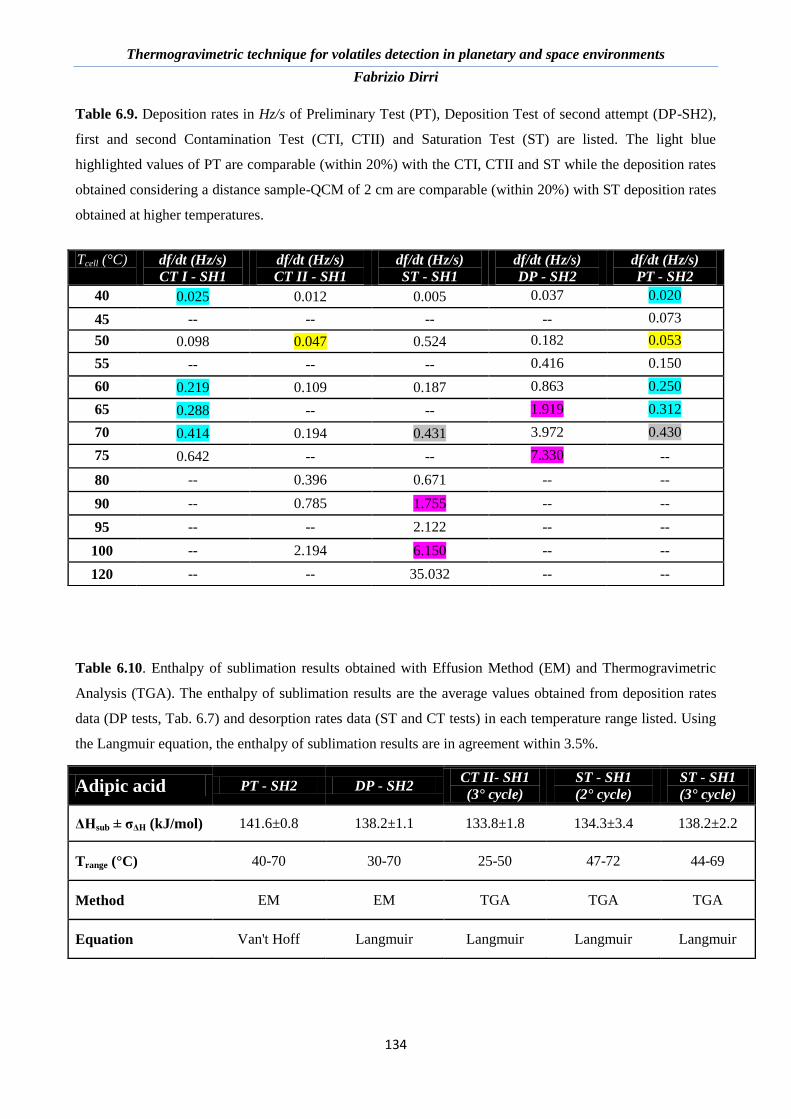
6.7. TGA, EM results and comparison ...................................................................................................... 133

Chapter 7. Conclusion ................................................................................................................................. 136

7.1. Calibration and experimental phase ................................................................................................... 136

7.2. Results and methods comparison ....................................................................................................... 137

7.3. Future perspectives ............................................................................................................................. 140

7.3.1. Laboratory Set-up improvements ................................................................................................ 140

7.3.2. Technological transfer application .............................................................................................. 142

7.3.3. ESA-M5 Call: proposed missions application ............................................................................. 144

Chapter 8. Bibliography ............................................................................................................................. 147

Appendix A - Publications .......................................................................................................................... 159

Appendix B - Scientific and Technological Projects ................................................................................. 162


Fabrizio Dirri

8


Fabrizio Dirri

9

Acronym List AEROSE AEROSOL AND OCEANOGRAPHIC SCIENCE EXPEDITION

AO ATOMIC OXYGEN

AOD AEROSOL OPTICAL DEPTH

ASAP-MS ATMOSPHERIC SOLIDS ANALYSIS PROBE MASS SPECTROMETRY

ASTM AMERICAN SOCIETY FOR TESTING MATERIALS

ATHENA ADVANCED TELESCOPE for HIGH ENERGY ASTROPHYSISCS

AVHRR ADVANCED VERY HIGH RESOLUTION RADIOMETER

BAM BETA ATTENUATION MONITORS

BB BREADBOARD

CALIOP CLOUD-AEROSOL LIDAR with ORTHOGONAL POLARIZATION

CALIPSO CLOUD-AEROSOL LIDAR AND INFRARED PATHFINDER SATELLITE OBSERVATIONS

CC CARBONACEOUS CHONDRITE

CNR ITALIAN NATIONAL RESEARCH COUNCIL

CQCM CRYOGENIC QUARTZ CRYSTAL MICROBALANCE

CT CONTAMINATION TEST

DC DOUBLE CRYSTAL

DNA DEOXYRIBONUCLEIC ACID

DS1 DEEP SPACE ONE

DT DEPOSITION TEST

EM EFFUSION METHOD

EMITS ELECTRONIC MAILING INVITATION TO TENDER SYSTEM

EOIM EVALUATION OF OXYGEN INTERACTION WITH MATERIALS EXPERIMENT

EPA ENVIRONMENTAL PROTECTION AGENCY

ESA EUROPEAN SPACE AGENCY

FOV FIELD OF VIEW

GHS GLOBAL HEAT SINK

HST HUBBLE SPACE TELESCOPE

IAPS INSTITUTE FOR SPACE ASTROPHYSISCS AND PLANETOLOGY

IECM INDUCED ENVIRONMENT CONTAMINATION MONITOR

IIA INSTITUTE OF ATMOSPHERIC POLLUTION

INAF NATIONAL INSTITUTE FOR ASTROPHYSICS

ISS INTERNATIONAL SPACE STATION

IUPAC INTERNATIONAL UNION OF PURE AND APPLIED CHEMISTRY

IVM INTEGRATED VOLUME METHOD

JAXA JAPAN AEROSPACE EXPLORATION AGENCY

JEM JOINT EUROPA MISSION

JUICE JUPITER AND ICY MOONS EXPLORER

KEM KNUDSEN EFFUSION MASS SPECTROMETRY

KEMS KNUDSEN EFFUSION MASS-loss

LEO LOW EARTH ORBIT

MBCs MAIN BELT COMETs

MEDET MATERIALS EXPOSURE AND DEGRADATION EXPERIMENT

MEU MAIN ELECTRONICS UNIT

MISR MULTI - angle IMAGING SPECTRORADIOMETER

MODIS MODERATE RESOLUTION IMAGING SPECTRORADIOMETER

MSX MIDCOURSE SPACE EXPERIMENT

NASA NATIONAL AERONAUTICS AND SPACE ADMINISTRATION

NEA NEAR EARTH ASTEROID

NI-DaQ NATIONAL INSTRUMENT DATA ACQUISITION

NIR NEAR INFRARED

OGO-6 ORBITING GEOPHYSICAL OBSERVATORY

OLEB ORIGIN OF LIFE AND EVOLUTION OF BIOSPHERES

OMI OZON MONITORING INSTRUMENT

PAH POLYCYCLIC AROMATIC HYDROCARBONS

PCM PIEZOELECTRIC CRYSTAL MICROBALANCE

PE PROXIMITY ELECTRONICS


Fabrizio Dirri

10

PIC PLUME IMPINGEMENT CONTAMINATION

PID PROPORTIANAL INTERGAL DERIVATIVE

PM PARTICULATE MATTER

POLDER POLARIZATION AND DIRECTIONALITY OF THE EARTH'S REFLECTANCES

PRCS PRIMARY REACTION CONTROL SYSTEM

PT PRELIMINARY TEST

PT-CIMS PROTON-TRANSFER CHEMICAL IONIZATION MASS SPECTROMETRY

PVC POLYVINYL CHLORIDE

QCM QUARTZ CRYSTALS MICROBALANCE

RCS REACTION CONTROL SYSTEM

REFLEX RETURN FLUX EXPERIMENT

RTD RESISTANCE TEMPERATURE DETECTOR

SAGEII STRATOSPHERIC AEROSOL and GAS EXPERIMENT II

SARE SOLAR ARRAY RETURN EXPERIMENT

SC SINGLE CRYSTAL

SEE ENVIRONMENTS and EFFECT

SEM SCANNING ELECTRONIC MICROSCOPE

SDS SMALL DEMONSTRATION SATELLITE

SH SENSOR HEAD

SMART SMALL MISSION FOR ADVANCED RESEARCH AND TECHNOLOGIES

SOA SECONDARY ORGANIC AEROSOL

SPICA SPACE INFRARED TELESCOPE for COSMOLOGY AND ASTROPHYSICS

SPIRIT SPATIAL INFRARED IMAGING TELESCOPE

SST SINGLE SCATTERING ALBEDO

ST SATURATION TEST

STS SPACE TRANSPORTATION SYSTEM

SVOC SEMI-VOLATILE ORGANIC COMPOUND

TCS TEMPERATURE CONTROL SYSTEM

TDMA TANDEM DIFFERENTIAL MOBILITY ANALYZER

TDPD TEMPERATURE PROGRAMMED THERMAL DESORPTION

TEC THERMO-ELECTRIC COOLER

TDPBMS TEMPERATURE PROGRAMMED THERMAL DESORPTION METHOD

TG THERMOGRAVIMETRY

TGA THERMOGRAVIMETRIC ANALYSIS

TQCM THERMAL QUARTZ CRYSTAL MICROBALANCE

TPTD THERMAL DESORPTION PARTICLE BEAM MASS SPECTROMETRY

TRL TECHNOLOGY READINESS LEVEL

TSMR THICKNESS SHEAR MODE RESONATOR

UI USER INTERFACE

Vis VISIBLE

VISTA VOLATILE IN-SITU THERMOGRAVIMETER ANALYSER

VOC VOLATILE ORGANIC COMPOUND

VTDMA VOLATILITY TANDEM DIFFERENTIAL MOBILITY ANALYSER

VVOC VERY VOLATILE ORGANIC COMPOUND

WSOC WATER-SOLUBLE ORGANIC COMPOUNDS

WHO WORLD HEALTH ORGANIZATION

XMM X-ray MULTI MIRROR MISSION


Fabrizio Dirri

11


Fabrizio Dirri

12

Chapter 1. Introduction

The study of minor bodies of the Solar System such as comets and asteroids is fundamental to understand

formation and early evolution of Solar System, including scenario of water delivery on the Earth. This

because most of the minor bodies are primitive, i.e. preserve information about the ancient solar nebula and

the first processes occurred. In particular, study of comets and asteroids received more attention thanks to the

recent missions such as the ESA mission Rosetta [Glassmeier 2007], the NASA missions NEAR-Shoemaker

[Williams 2001] and Dawn [Russell and Raymond 2011], the JAXA Hayabusa 1[Kubota 2006]. The Rosetta

mission flayed over the Asteroid 2867 Šteins e 21Lutetia and studied in detail the comet 67P/Churyumov-

Gerasimenko giving some important results about the nucleus, dust and gas composition. The NASA NEAR-

Shoemaker Mission which has studied in depth the surface composition and geomorphology of the Asteroid

433 Eros . The NASA Dawn Mission whose targets were the giant asteroids 4Vesta and 1 Ceres. Finally, the

JAXA Hayabusa 1 mission mapped the asteroid Itokawa studying its surface geology and mineral

composition and returned to Earth fragments of its regolith.

In addition, Sample Return Missions such as JAXA Hayabusa 2 [Tsuda 2013] and NASA Osiris-REx [Barry

2013] are in progress and are addressed to two primitive asteroids, i.e. 101955 Bennu and 162173 Ryugu,

respectively. These missions will help the characterization and classification of these bodies and most

importantly will return pristine material to the Earth laboratories.

In the last Call for a Medium-size mission opportunity in ESA's Science Program (M5), many missions to

minor bodies are proposed: theMarcoPolo-M5 (Sample Return Mission from a primitive asteroid, i.e. 1993

HA), Akon and JEM (Europa target) and Castalia (Main Belt Comets target) will be helpful for the

characterization of Asteroids and Comets.

Volatiles detection and characterization is required during the outgassing processes which occur in space

environment aboard satellites, spacecraft and space stations (e.g. ISS, Mir) [Soares 2003, Soares and

Mikatarian 1994]. Indeed, it is well-known that observed phenomena as surface erosion (e.g. by Atomic

Oxygen, AO), weight loss, oxidation and surface bombardment (e.g. thruster firings) can degredates the

performance of telescope, optics and other sensible parts of scientific instruments [de Chambure 1997]. On

the other hand, volatiles detection in the minor bodies of Solar System and in planetary atmospheres

represent a good opportunity to understand the mineralogical history of the processes concerning the

evolution and the transformation processes in atmosphere in order to characterize the organic fraction of

atmospheric aerosols. Furthermore, specific substances (markers) can be identified in order to provide some

information on the atmospheric aerosol sources (biogenic or anthropogenic, i.e. on the Earth) [Bacco 2010,

Dirri 2016a]. In this sense, the study and monitoring of the thermodynamical and thermochemical processes

and parameters useful to characterize a compound or a mix of them should be taken into account.


Fabrizio Dirri

13

This work has been performed in the Volatile In-Situ Thermogravimeter Analyser (VISTA) activity

framework which aims at developing an instrument to detect volatiles in planetary and space environments

[Palomba 2016]. The project is led by IAPS-INAF and developed by a consortium of three Italian institutes

and one Industry. This work has take advantage of the collaboration between the VISTA-team members.

Two main project are included in these activity: Contamination Assessment Microbalance (CAM), an

Electronic Mailing Invitation to Tender System of European Space Agency (EMITS-ESA) Project aiming a

development of thermogravimeter for contamination measurements in space and VISTA-MarcoPoloR

[Palomba 2012] which aims at develop a thermogravimeter for a planetary in-situ mission on primitive

asteroid.

VISTA is a miniaturized thermogravimeter system based on Thermogravimetric Analysis (TGA), a widely

used technique to investigate deposition/sublimation and absorption/desorption processes of volatile

compounds in different environments: outgassing contamination in space, dehydration and organic

decomposition in minerals [Grady and Wright 2003, Fermo 2006]. It measures the change in mass of a

sample as a function of temperature and time. The VISTA main innovation introduced is the PCM special

design equipped with two built-in resistors, placed on the opposite faces on the crystal, acting as heater and

temperature sensor, respectively.VISTA is composed of two sensor heads, i.e. the Sensor Head 1 (SH1) for

in-orbit contamination measurements from outgassing processes and Sensor Head 2 (SH2) for planetary in-

situ measurements, respectively [Palomba 2016]. Each sensor head includes a sensing piezoelectric crystal

and related Proximity Electronics (PE).

A Engineering Model and laboratory breadboard of SH1 were developed in a EMITS-ESA Project, i.e.

CAM, which aim to design and develop a instrument for space contamination monitoring for the future ESA

payloads. For SH2, a laboratory breadboard has been developed, too.

VISTA can accomplish the following scientific goals:

a. measurement of the abundance of volatiles and organics in the asteroid regolith and measuring the

water content in the hydrate minerals;

b. measurement the cometary activity or the possible cometary-like activity;

c. monitoring sampling operations by measuring the flux of dust raised;

d. monitoring a contaminant source, simulating an outgassing process in space environment;

e. characterizing a contaminant source by realizing TGA cycles to obtain the vapor pressures and

enthalpy of sublimation;

f. evaluating the degradation of the instrumentation performance by means of the measured mass

deposited on the crystal surface.

A first phase of the work was based on Volatile Organic Compounds (VOCs) study in planetary atmospheres

including their physical-chemical properties and their connections with the atmospheric aerosol sources.


Fabrizio Dirri

14

Simultaneously, a study of VOCs detection in space come from outgassing processes of materials exposed

to space environment and the related instrumentation issues was studied in depth.

Successively, a complete study of TGA and thermochemical processes as well as a complete review for

Quartz Crystal Microbalance (QCM) sensors used for contamination in space were performed. Thus, vapor

pressures and enthalpy of sublimation were identified as those thermochemical parameters able to

characterize a kinetics process regarding VOCs in planetary atmosphere and in space. A laboratory activity

was divided in a first design and development phase of two laboratory setup and in a second calibration

phase of VISTA sensor heads. A third phase was devoted to performing different tests for contamination

study in space (using a contaminant source and SH1 breadboard) and for VOCs characterization in

atmosphere (using five dicarboxylic acids and SH2 breadboard). The dicarboxylic acids have been chosen

due to their high sublimation rates starting from 25-30°C which make them a good contaminant source and

due to their presence in the organic materials of CC (come from primitive asteroids) and in Secondary

Organic Aerosol (SOA) of terrestrial atmosphere.

The work of the thesis is divided in seven chapters. The first chapter aims to introduce the work performed

while the second chapter gives a description about VOCs and their detection in terrestrial atmospheric SOA

(as organic fraction) and in space (as contaminant), especially focusing the attention on dicarboxylic acid

compounds and their chemical-physical properties.

In the third chapter, the thermochemical relations, the physical-chemical quantity for organic compounds

characterization are introduced. The basic concept of Thermogravimetry, the working principle of

microbalance system for laboratory-use and VISTA sensor heads (SH1 and SH2) are explained in detail.

The fourth chapter gives a description of the two experimental setups designed, developed and tested for

contamination tests performed with the SH1 breadboard and for atmospheric organic compounds

characterization with the SH2 breadboard. Thermal tests, User Interface (UI) to manage the SH1 and SH2,

vacuum system and experimental procedures are described.

The fifth chapter describes the contamination and saturation tests performed with SH1 breadboard, the data

analysis and the experimental procedure performed using a contamination source with a sufficient

sublimation rates from 25-30°C, i.e. the adipic acid. Different TGA cycles are performed (with the built-in

heaters) to regenerate the crystals and obtaining a characterization of the source by means of the enthalpy of

sublimation using the Langmuir equation. The results has been discussed and compared with previous works.

In the sixth chapter, in preparation for organic compounds characterization with SH2, the TGA data set

obtained with SH1 have been used to obtain the vapor pressures and the enthalpy of sublimation using

Clausius-Clapeyron equation. Thus, the SH2 experimental activity, i.e. deposition tests obtained with the


Fabrizio Dirri

15

Effusion Method (EM) are introduced. Calibration test, experimental procedure and data analysis are

described as well as the results of deposition rates and enthalpy of sublimation obtained (with Van't Hoff

equation) for five compounds, i.e. oxalic acid, succinic acid, adipic acid, suberic acid and azelaic acid. The

results have been discussed and compared with previous works. In particular, the enthalpy of sublimation

obtained with Langmuir and Clausius-Clapeyron equation and SH1 breadboard (TGA method) have been

compared with enthalpy average value obtained with Van't Hoff equation and SH2 breadboard (EM).

In the seventh chapter, the laboratory work and the results (deposition rates and enthalpy of sublimation)

obtained with different methods (TGA and EM) and breadboards (SH1 and SH2) are summarized. A

complete list of future applications, i.e. for Space Missions (ESA-M5) and Transfer Technological

Application (terrestrial atmosphere, farming business, pharmaceutical area etc.) relating to VISTA sensor

heads following the results of this thesis are described.


Fabrizio Dirri

16


Fabrizio Dirri

17

Chapter 2. VOCs in terrestrial atmosphere and space

2.1 Introduction

Volatile Organic Compounds (VOCs) in terrestrial atmosphere and in space detection including their

physical-chemical processes are introduce in this chapter.

The different types of atmospheric aerosols and VOCs are described as well as the importance of their

detection in atmosphere because of their influence on the climate. In particular, markers for the Secondary

Organic Aerosol (SOA) characterization, i.e. dicarboxylic acid are identified and their chemical-physical

properties are introduced.

VOCs detection in space originate from material outgassing processes exposed to vacuum environment and

high temperature variations are also introduced. The instrumentation issues related to the contamination

processes and a review of contamination measurement performed on ISS and Mir Station and aboard

satellites and spacecraft are illustrated.

The detection of volatile materials in the planetary bodies, i.e. from comets and asteroids and their

connection with analogue materials are discussed (in particular, focusing the attention on dicarboxylic acid

compounds related to these analogue materials).

2.2. Terrestrial atmospheric aerosols

Aerosol system is a liquid and/or solid particles (diameter from 10-9

to 10-4

m) in a carrier gas. It is generally

defined as a solid suspension of liquid or solid particles in a gas able to scatter and absorb sunlight if

sufficient large [Rozaini 2012]. Aerosols interact both directly and indirectly with the Earth's radiation

budget (the aerosols scatter sunlight directly back into space) having a direct effect on climate. Because of

the large number of aerosol species in atmosphere and physical-chemical processes which occur to

create/destroy compounds, a complete characterization and monitoring of them is a tricky task. Thus, it is

necessary to identify a specific substances or a class of substances (i.e. "markers") able to provide

information about the sources (biogenic or anthropogenic) which generates the Particulate Matter (PM)

(microscopic solid or liquid particles suspended in atmosphere) in the aerosol and their permanence in

atmosphere [Bacco 2010]. Because of aerosols change their characteristics very slowly, they can be used as

tracers for atmospheric motions and generally to understand how the Earth's atmosphere moves [NASA

1996]. For example, atmospheric aerosols have been used to study the dynamics of the polar regions and the

exchange of air between the troposphere and stratosphere. Three types of aerosols are mainly present at

Earth's atmosphere and affect the climate:

1. Background aerosol (aged accumulation mode aerosol, i.e. volcanic aerosol), which forms a layer in the

stratosphere after volcanic eruptions (sulfur dioxide gas).

2. Maritime aerosol, a main component of which is sea salt.


Fabrizio Dirri

18

3a. Continental aerosol, i.e. desert dust, minute grains of dirt blown from the desert surface (clay minerals

dust).

3b. Continental aerosol, human-made aerosol, coming from process as rock erosion, smoke from burning

tropical forests (rural aerosol) and from human vehicles, industries etc. (urban aerosols, these particles can

affect the heart and lungs and cause serious health effects. Generally, urban and rural aerosols are also

identified as "primary atmospheric aerosol".

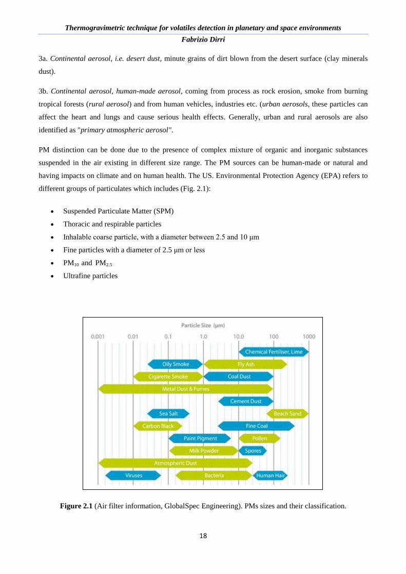
PM distinction can be done due to the presence of complex mixture of organic and inorganic substances

suspended in the air existing in different size range. The PM sources can be human-made or natural and

having impacts on climate and on human health. The US. Environmental Protection Agency (EPA) refers to

different groups of particulates which includes (Fig. 2.1):

Suspended Particulate Matter (SPM)

Thoracic and respirable particles

Inhalable coarse particle, with a diameter between 2.5 and 10 μm

Fine particles with a diameter of 2.5 μm or less

PM10 and PM2.5

Ultrafine particles

Figure 2.1 (Air filter information, GlobalSpec Engineering). PMs sizes and their classification.


Fabrizio Dirri

19

A significant contribution to atmospheric aerosol particles is the product formation of low volatility and

chemically processed Volatile Organic Compound (VOCs). By means of photochemical and oxidation

processes, VOCs are transformed to less volatile contributing to Secondary Organic Aerosol (SOA) [Salo

2010]. The physical pathways and identification of the low-volatility products originating from oxidation of

VOCs are not fully understood even though it is know that typical class of products from atmospheric

oxidation processes yielding SOA are the carboxylic acids class which includes a subclass: dicarboxylic

acids.

The atmospheric aerosol study has a scientific relevance due to connection between the public health and to

the particulate exposition, in particular the ultra-thin organic component of PM2.5 and PM10 [Ladji 2007]. The

origin of atmospheric pollutants source becoming more important on the basis of current EU Directive of

2008 on ambient air quality and cleaner air for Europe explicitly states that: “emissions of harmful air

pollutants should be avoided, prevented or reduced and appropriate objectives set for ambient air quality

taking into account relevant World Health Organization standards, guidelines and programmes” [EU 2008].

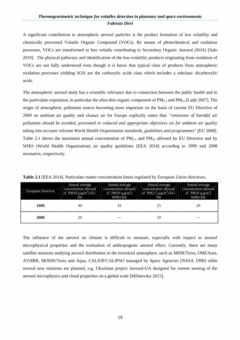
Table 2.1 shows the maximum annual concentration of PM2.5 and PM10 allowed by EU Directive and by

WHO (World Health Organization) air quality guidelines [EEA 2014] according to 1999 and 2008

normative, respectively.

Table 2.1 [EEA 2014]. Particulate matter concentration limits regulated by European Union directives.

European Directive

Annual average

concentration allowed

of PM10 (μg/m3) EU-

Dir

Annual average


of PM10 (μg/m3)

WHO-Dir

Annual average


of PM2.5 (μg/m3) EU-

Dir

Annual average


of PM10 (μg/m3)

WHO-Dir

1999 40 10 25 20

2008 20 -- 10 --

The influence of the aerosol on climate is difficult to measure, especially with respect to aerosol

microphysical properties and the evaluation of anthropogenic aerosol effect. Currently, there are many

satellite missions studying aerosol distribution in the terrestrial atmosphere, such as MISR/Terra, OMI/Aura,

AVHRR, MODIS/Terra and Aqua, CALIOP/CALIPSO managed by Space Agencies [NASA 1996] while

several new missions are planned, e.g. Ukrainian project Aerosol-UA designed for remote sensing of the

aerosol microphysics and cloud properties on a global scale [Milinevsky 2015].


Fabrizio Dirri

20

2.2.1. VOC and SOA

The EPA definition of VOC means any compound of carbon, excluding carbon monoxide, carbon dioxide,

carbonic acid, metallic carbides or carbonates and ammonium carbonate, which participates in atmospheric

photochemical reactions, except those designated by EPA as having negligible photochemical reactivity

[EPA 2016].

VOCs are those organic compounds whose composition makes it possible for them to evaporate under

normal indoor atmospheric conditions of temperature and pressure. The volatility of organic compounds are

defined and classified by their boiling points because the volatility generally increase when boiling point

temperature is lower (VOC have a boiling point less than 250°C at 101.3 kPa) [EPA 2016]. VOCs are

sometimes categorized by the ease they will be emitted. For example, WHO categorizes the indoor organic

pollutants [WHO 1987] as:

Very volatile organic compounds (VVOCs)

Volatile organic compounds (VOCs)

Semi-volatile organic compounds (SVOCs)

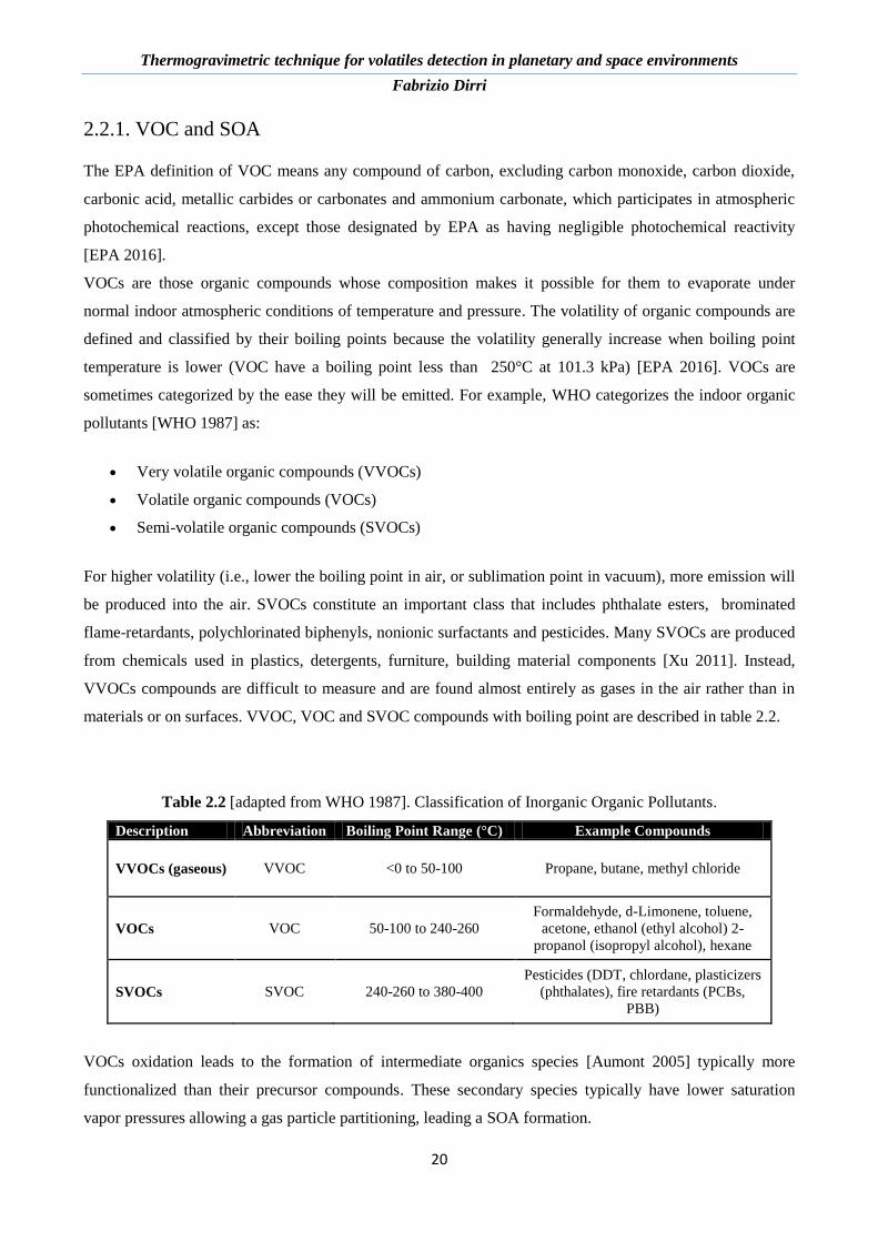
For higher volatility (i.e., lower the boiling point in air, or sublimation point in vacuum), more emission will

be produced into the air. SVOCs constitute an important class that includes phthalate esters, brominated

flame-retardants, polychlorinated biphenyls, nonionic surfactants and pesticides. Many SVOCs are produced

from chemicals used in plastics, detergents, furniture, building material components [Xu 2011]. Instead,

VVOCs compounds are difficult to measure and are found almost entirely as gases in the air rather than in

materials or on surfaces. VVOC, VOC and SVOC compounds with boiling point are described in table 2.2.

Table 2.2 [adapted from WHO 1987]. Classification of Inorganic Organic Pollutants.

Description Abbreviation Boiling Point Range (°C) Example Compounds

VVOCs (gaseous) VVOC <0 to 50-100 Propane, butane, methyl chloride

VOCs VOC 50-100 to 240-260

Formaldehyde, d-Limonene, toluene,

acetone, ethanol (ethyl alcohol) 2-

propanol (isopropyl alcohol), hexane

SVOCs SVOC 240-260 to 380-400

Pesticides (DDT, chlordane, plasticizers

(phthalates), fire retardants (PCBs,

PBB)

VOCs oxidation leads to the formation of intermediate organics species [Aumont 2005] typically more

functionalized than their precursor compounds. These secondary species typically have lower saturation

vapor pressures allowing a gas particle partitioning, leading a SOA formation.


Fabrizio Dirri

21

SOA is mainly composed of fine particles, i.e. lower than 1-2μm, [Salzen and Schlṻnzen 1999] from photo-

oxidation reactions with compounds in Earth's atmosphere, in particular hydroxyl radical, ozone and nitrate

radical. For example, hydrocarbons are enriched carboxyl (-COOH), carbonyl (-CO) or hydroxyl (-OH)

functional groups are transformed in ketones or carboxylic acid after several reactions. SOA formation

involves a multitude of Semi-Volatile Organic Compounds (SVOC) having complex molecular structures.

SVOC formation is suspected to be more complex with the possibility of multiple oxidation steps [Kroll and

Seinfeld 2005].

Figure 2.2 [Camredon et al. 2007]. Schematic diagram of SOA formation. The number "1" was referred to

1-octene oxidation studied.

SVOC production might require many successive oxidation steps which provide minor individual

contribution to the organic budget. In particular, the model assumed for SOA formation includes the

production of "i" species by means of single oxidation step from parent hydrocarbons and a specific

thermodynamic module for condensation (Fig. 2.2). The oxidation scheme up to CO2 production has been

developed using the self-generation approach of Aumont (2005) and assuming a basic thermodynamic

absorption process [Pankow 1994] for gas/particles partitioning of low volatility species.

2.2.2. Organic fraction of VOC and SOA

Generally, a lot of aerosols transformation processes occur in the terrestrial atmosphere. Aerosols are largely

composed by inorganic species but a significant fraction of the total particulate matter is composed of

organics. These substances are typically mixed to inorganic compounds and has been determined that


Fabrizio Dirri

22

organics usually constitute 20-50% of fine aerosol mass over the continental U.S. [Brown 2013]. Organics

may also constitute a significant fraction of atmospheric aerosol even at high altitudes, which may be

important for ice formation in clouds [Salo 2010] showing an important role on atmospheric aerosol

formation and growth (due to its hygroscopic characteristic, toxicity and radiation absorption). Rogge (1993)

identified more than 80 organic compounds in atmospheric particles, including Dicarboxylic acids (identified

in cloud water samples). The occurrence of Polycyclic Aromatic Hydrocarbons (PAH), could be cause of

concern, due to their carcinogenic effects. Generally, organic compounds are related to species contains

between 5 and 10 carbon atoms (C5-C10), since the species with higher carbon atoms have low

concentrations, low molecular weight and high vapor pressure [Barthelmie 1997]. The organic fraction of

SOA can be formed by biogenic (80% of VOC) and anthropogenic precursor: species as O3 and H-O

(hydroxyl radical) can transform group contains hydrocarbon in carboxylic group (-COOH) and carbonyl

group (-CO) or hydroxyl (OH) compounds enriched. These reaction lead to formation of ketones, carboxylic

acids etc. Furthermore, in different samples of urban, rural and sea aerosol have been identify alkanes longer

chain, ketones, different salts, dicarboxylic acid and PAH.

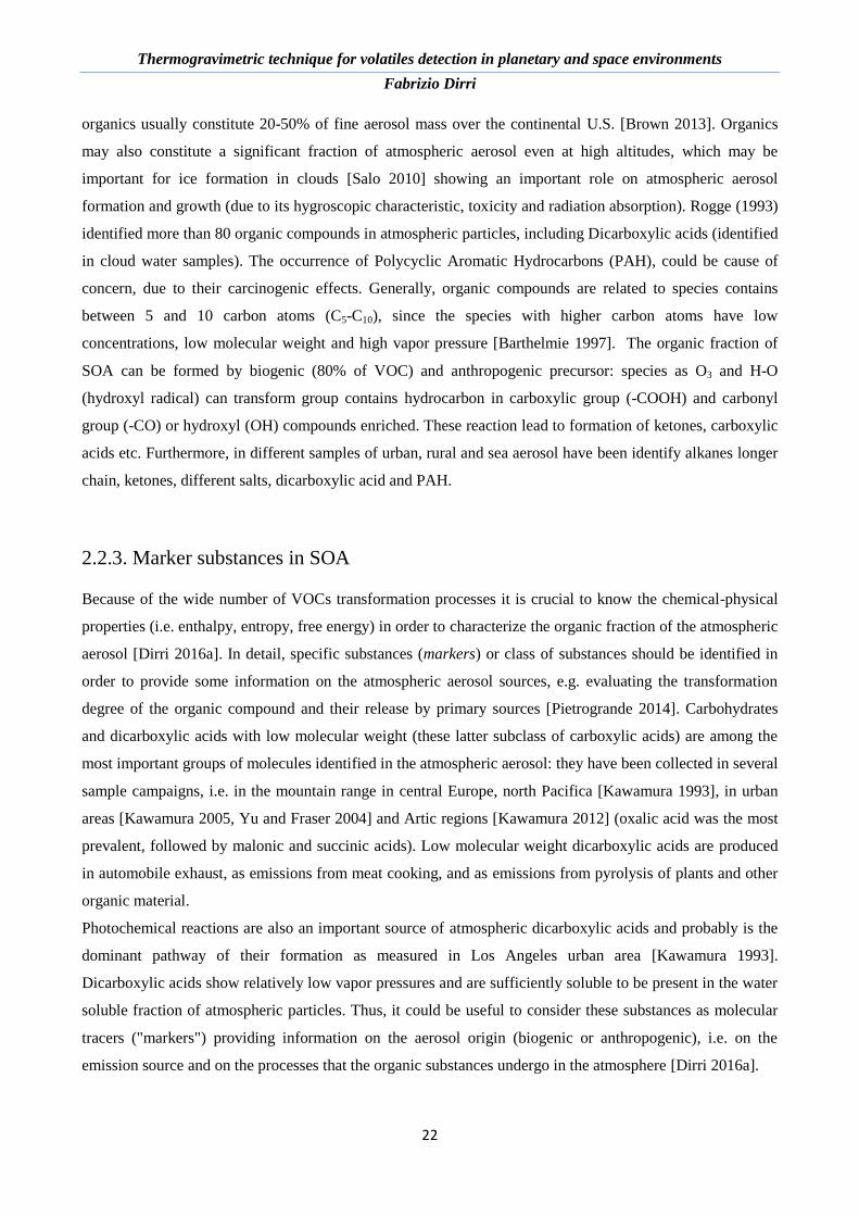
2.2.3. Marker substances in SOA

Because of the wide number of VOCs transformation processes it is crucial to know the chemical-physical

properties (i.e. enthalpy, entropy, free energy) in order to characterize the organic fraction of the atmospheric

aerosol [Dirri 2016a]. In detail, specific substances (markers) or class of substances should be identified in

order to provide some information on the atmospheric aerosol sources, e.g. evaluating the transformation

degree of the organic compound and their release by primary sources [Pietrogrande 2014]. Carbohydrates

and dicarboxylic acids with low molecular weight (these latter subclass of carboxylic acids) are among the

most important groups of molecules identified in the atmospheric aerosol: they have been collected in several

sample campaigns, i.e. in the mountain range in central Europe, north Pacifica [Kawamura 1993], in urban

areas [Kawamura 2005, Yu and Fraser 2004] and Artic regions [Kawamura 2012] (oxalic acid was the most

prevalent, followed by malonic and succinic acids). Low molecular weight dicarboxylic acids are produced

in automobile exhaust, as emissions from meat cooking, and as emissions from pyrolysis of plants and other

organic material.

Photochemical reactions are also an important source of atmospheric dicarboxylic acids and probably is the

dominant pathway of their formation as measured in Los Angeles urban area [Kawamura 1993].

Dicarboxylic acids show relatively low vapor pressures and are sufficiently soluble to be present in the water

soluble fraction of atmospheric particles. Thus, it could be useful to consider these substances as molecular

tracers ("markers") providing information on the aerosol origin (biogenic or anthropogenic), i.e. on the

emission source and on the processes that the organic substances undergo in the atmosphere [Dirri 2016a].


Fabrizio Dirri

23

2.2.4. Continental and background aerosols monitoring

Although the aerosol measurement and monitoring is improved during the last decades, many questions are

already open about the competing impacts of aerosols. For example, measuring the particles within clouds

remains challenging because of different types of particles can clump together to form hybrids that are

difficult to distinguish. During the last years, the scientist have used an array of satellite, aircraft, and

ground-based instruments to monitor aerosols, e.g. the radiometer instruments which are able to quantify the

amount of electromagnetic radiation. Some properties such as Aerosol Optical Depth (AOD), i.e. a measure

of the amount of light that aerosols scatter and absorb in the atmosphere or Single Scattering Albedo (SSA),

i.e. the fraction of light that is scattered compared to the total are the main quantities measured [NASA Earth

Observatory 2016]. Satellites to monitor the AOD and in the Visible (Vis) and Near-Infrared (NIR)

spectrum, i.e. the Advanced Very High Resolution Radiometer (AVHRR) and to view and study aerosols at

more angles and wavelengths, i.e. the Multi-angle Imaging Spectroadiometer (MISR) and the Moderate

Resolution Imaging Spectroradiomer (MODIS) have been used [Mishchenko 2007, Remer 2008]. Other

instruments such as the Cloud Aerosol Lidar and Infrared Pathfinder Satellite Observer (CALIPSO) and the

Polarization and Directionality of the Earth’s Reflectances (POLDER) are able to measure in detail the

vertical profiles of aerosol (in the plumes and clouds) and the orientation (or polarization) of light waves and

their movement through the atmosphere, respectively [NASA Earth Observatory 2016].

In particular, the studying on continental aerosol due to desert dust (e.g. Saharan dust) it's important to

understand the microphysical evolution of thin particles from the source regions with reactive gas phase

species during the long distance transport [Effiong 2011]. These properties could change the chemistry of the

troposphere influencing the radiative transfer and optical properties [Otto 2007].

The PCM sensors, in particular the Quartz Crystal Microbalance (QCM) can be used for atmospheric

monitoring, e.g. AEROSE mission. The objective of Aerosol and Oceanographic Science Expedition

(AEROSE) was to provide measurements about the dust Sahara storm and on the influence of dust particles

on atmospheric and oceanographic properties during trans-Atlantic transport. QCMs were used as deposition

surface for different types of particles (PM2.5 and PM10), in order to realize in situ real time measurement

sample in various portion of the dust plume that occurred over the tropical Atlantic Ocean [Effiong 2011].

Two QCM’s have been placed inside the Howard University Van located at 8 m above mean sea level on an

Oceanographic ship. By means of Scanning Electron Microscope (SEM) analysis has been shown that they

are able to obtain a smaller samples with an high resolution in its measurements that view the size fraction of

0.15, 0.3, 0.6, 1.2 and 5.0 μm. In figure 2.3 (at Right) it is possible to observe the size particles distribution

before the dust storm (QCM data1) and the evolution (at Left) of the particles during the storm exposure

(QCM data2, March 5-7, 2004).


Fabrizio Dirri

24

Figure 2.3 [Morris and Roldan 2005]. Left: atmospheric PM before the dust storm. The particulate was

between 2.5 and 0.3 μm with the peak at 1.2 μm. Right: evolution of the PM detected by QCM2; the PM

detected are PM2.5 and PM1.2 with a peak near 0.3 μm.

Beforehand dust storm, the aerosol dust density (March 5th) had a peak in the 1.2 micron size range while

during the storm (March 7th) a double distribution was observed in the 1.2 and 0.5 micron size range.

By means of a QCMs the flux of PM10 and PM2.5 were measured (in μg/m3) during the AEROSE campaigns.

SEM analysis confirmed the results and the capability of the QCM to reveal the different particulate. Then,

the AEROSE team encountered several dust event and completed the different measurements, giving a

unique and valuable open ocean data set, obtaining a data on the aerosol properties during and after the event

[Morris and Roldan 2005].

On the other hand, the background aerosol (i.e. volcanic aerosol) deposited into stratosphere during several

decades is also largely studied due to change the chemistry and reducing the amount of energy reaching the

lower atmosphere and the Earth's surface, cooling them. Data from satellites such as the NASA Langley

Stratospheric Aerosol and Gas Experiment II (SAGE II) have enabled scientists to better understand the

effects of volcanic aerosols on our atmosphere [NASA 1996].

The study of volcanic solid particles present in atmosphere and the composition of volatile outgassed species

before and after a strong volcanic eruptions could be useful to provide information about the time evolution

of the volcanic activity [Casadevall 1984].

Currently, the substances monitoring emitted in volcanic areas is based on accumulation chambers which

collect the gaseous mixture coming from underground, while systems aimed at detecting volcanic particulate

are not available. The major producers of these systems are LI-COR BIOSCIENCES (USA), WEST

SYSTEM (Italy), PASI (Italy), ADC BioScientific (UK) (with costs range: from 4000 up to 10000€). In this

framework, a PCM device can be used with a coated material (i.e. metals) in order to reveal the volcanic

gases which can be corrode the metal (e.g. gold). In addition, PCM would allow the continuous measurement

of PM, too while the small dimensions makes it easy to install in different places of the volcanic area.


Fabrizio Dirri

25

Generally, the aim of the scientists for the next future is to reduce the quantitative uncertainties on the

amount of aerosol (especially on the aerosol properties). Indeed, thermochemical properties will help to

know the aerosols behavior in the terrestrial atmosphere providing a critical information to understand the

aerosol impacts into climate models (thanks to sophisticated computer modeling) and to reduce the

uncertainties about how the climate is influenced by aerosols.

2.3. VOC detection in space

Spacecraft contamination from volatile desorption is one the main problem that engineers have to take into

account when developing a new satellites. Indeed, the solar radiation and instantaneously thermal variation

induced a difference behavior of materials which results as outgassing processes. By several decades, one of

the aim of National Aeronautics and Space Administration (NASA) and European Space Agency (ESA) was

to monitor the outgassing properties of aerospace materials based on ground and testing the outgassing

effects on spacecraft in flight [Green 2001].

During the next decades, the contamination around Satellite and Space Shuttle missions have been

monitored. In fact, when spacecrafts proceeds from Earth environments to space environment, the major part

of the satellite components can degas and major flux of contaminant can deposited on the spacecraft surfaces

or on the sensitive component of instruments (e.g. optics). In addition, the cabin leakage, thruster firings and

the solar effects complicate the contamination detecting and data analysis on ground.

Generally, for contamination detection, QCM's have been used on spacecrafts and satellites (for on-orbit

measurements of contaminations level), in various Shuttle mission (STS) and in new technologies interest

missions, e.g. Midcourse Space Experiment (MSX). The first task to avoid contamination was to accumulate

data from facilities using QCMs to measure the outgassing rates for satellite materials. Specially, the

American Society for Testing Materials (ASTM) E-1559 standard method (established procedure in 1993)

[Garrett 1995] has been used to evaluate the satellite materials outgassing. This test method allows the total

mass loss to be determined through the use of 2 to 4 quartz crystal microbalances cooled to various

temperatures [Green 2001]. In particular, two procedures (A and B) can be used for determining the

outgassing kinetics. Method A can use a standard effusion cell temperatures and three QCMs cooled at 90,

160, and 298K while the source temperature was 125°C [Garrett 1995]. The geometries provide a standard

view factors form the QCMs to the effusion cell orifice (Fig. 2.4). The B procedure, shows a considerable

flexibility considering the experimental parameters, in particular the set-point temperatures and test

geometry. Basically, the user can perform a custom test using specific parameters or modified apparatus

[Green 2001].


Fabrizio Dirri

26

Figure 2.4 [Garrett 1995]. Schematic view of QCM collection measurement with ASTM E-1559 method.

The QCMs are optically polished with resonant frequency of 10 to 15 MHz and are angled of 10° from their

axis. The intersection point (the effusion cell orifice exit plane) is at 150 mm from the crystal surface. The

liquid nitrogen reservoirs is able to cool the QCMs down to 90K.

A database of outgassing kinetics parameters have been created and managed by NASA's Space

Environments and Effect (SEE) Program Office located a t the Marshall Space Flight Center in Huntsville,

Alabama [Green 2001].

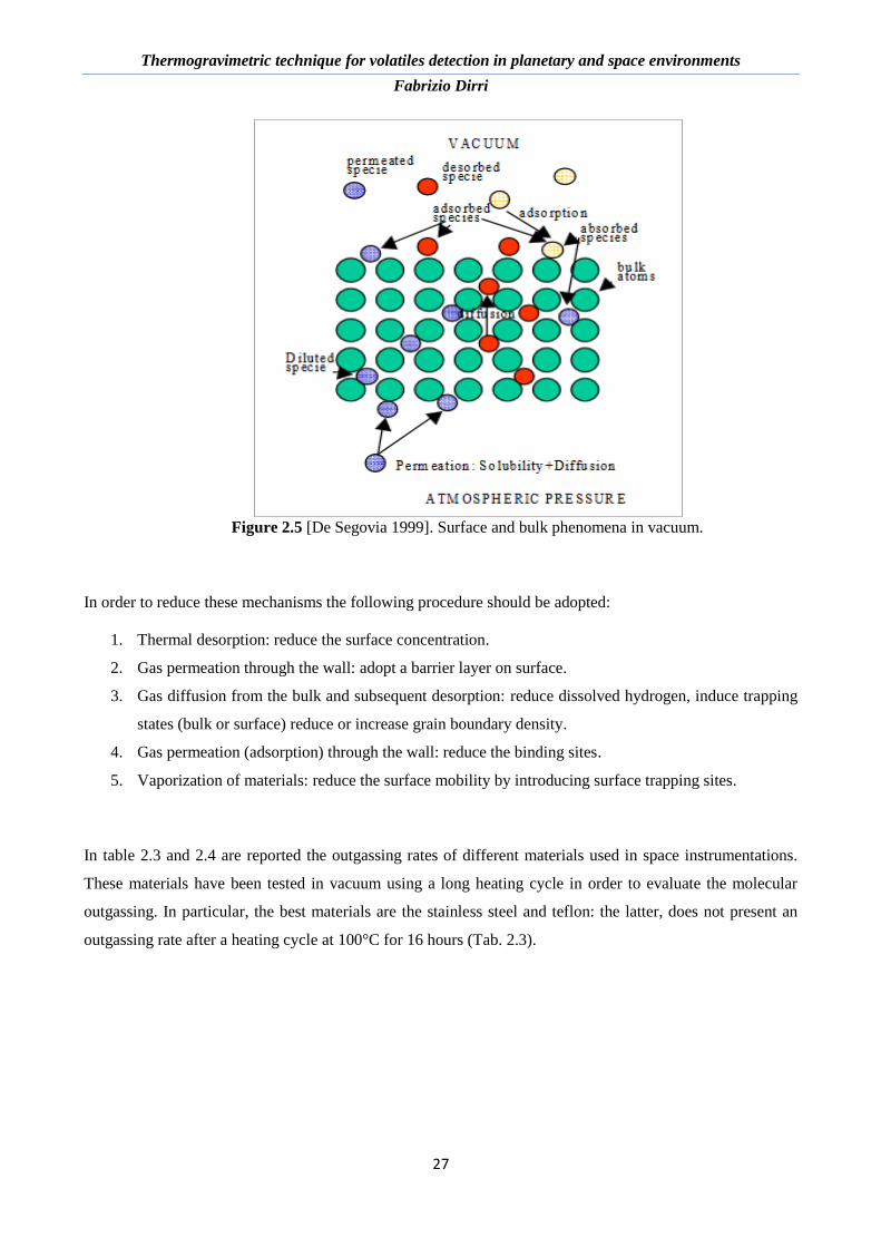
2.3.1. Outgassing process and instrument issues

Generally, the gassing and outgassing are recognized as gas controlled processes in high and ultra-high

vacuum system. The mechanisms contributing to outgassing processes are [De Segovia 1999] (Fig. 2.5):

1. Thermal desorption

2. Gas permeation through the wall

3. Gas diffusion from the bulk and subsequent desorption

4. Gas permeation (adsorption) through the wall

5. Vaporization of materials


Fabrizio Dirri

27

Figure 2.5 [De Segovia 1999]. Surface and bulk phenomena in vacuum.

In order to reduce these mechanisms the following procedure should be adopted:

1. Thermal desorption: reduce the surface concentration.

2. Gas permeation through the wall: adopt a barrier layer on surface.

3. Gas diffusion from the bulk and subsequent desorption: reduce dissolved hydrogen, induce trapping

states (bulk or surface) reduce or increase grain boundary density.

4. Gas permeation (adsorption) through the wall: reduce the binding sites.

5. Vaporization of materials: reduce the surface mobility by introducing surface trapping sites.

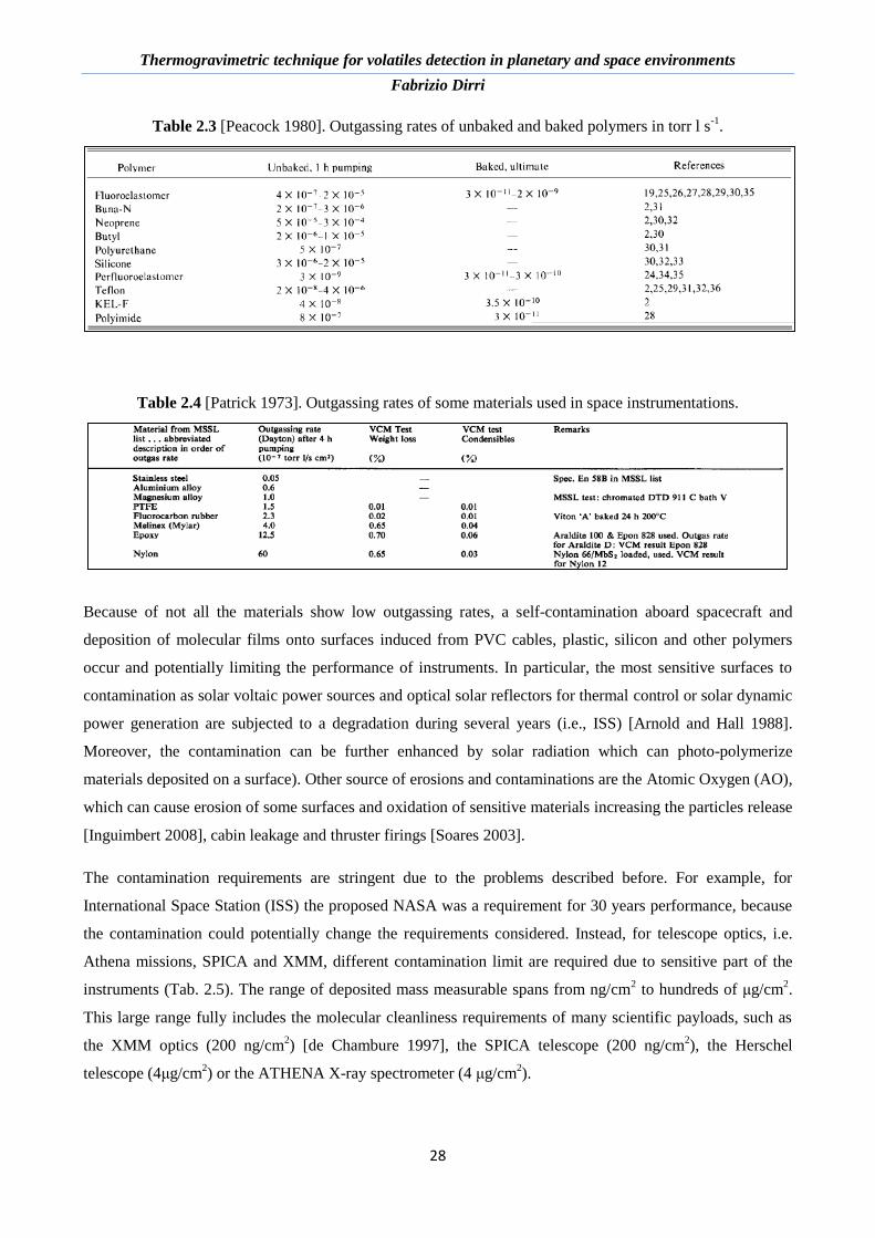
In table 2.3 and 2.4 are reported the outgassing rates of different materials used in space instrumentations.

These materials have been tested in vacuum using a long heating cycle in order to evaluate the molecular

outgassing. In particular, the best materials are the stainless steel and teflon: the latter, does not present an

outgassing rate after a heating cycle at 100°C for 16 hours (Tab. 2.3).


Fabrizio Dirri

28

Table 2.3 [Peacock 1980]. Outgassing rates of unbaked and baked polymers in torr l s-1

.

Table 2.4 [Patrick 1973]. Outgassing rates of some materials used in space instrumentations.

Because of not all the materials show low outgassing rates, a self-contamination aboard spacecraft and

deposition of molecular films onto surfaces induced from PVC cables, plastic, silicon and other polymers

occur and potentially limiting the performance of instruments. In particular, the most sensitive surfaces to

contamination as solar voltaic power sources and optical solar reflectors for thermal control or solar dynamic

power generation are subjected to a degradation during several years (i.e., ISS) [Arnold and Hall 1988].

Moreover, the contamination can be further enhanced by solar radiation which can photo-polymerize

materials deposited on a surface). Other source of erosions and contaminations are the Atomic Oxygen (AO),

which can cause erosion of some surfaces and oxidation of sensitive materials increasing the particles release

[Inguimbert 2008], cabin leakage and thruster firings [Soares 2003].

The contamination requirements are stringent due to the problems described before. For example, for

International Space Station (ISS) the proposed NASA was a requirement for 30 years performance, because

the contamination could potentially change the requirements considered. Instead, for telescope optics, i.e.

Athena missions, SPICA and XMM, different contamination limit are required due to sensitive part of the

instruments (Tab. 2.5). The range of deposited mass measurable spans from ng/cm2 to hundreds of μg/cm

2.

This large range fully includes the molecular cleanliness requirements of many scientific payloads, such as

the XMM optics (200 ng/cm2) [de Chambure 1997], the SPICA telescope (200 ng/cm

2), the Herschel

telescope (4μg/cm2) or the ATHENA X-ray spectrometer (4 μg/cm

2).


Fabrizio Dirri

29

Table 2.5. The Space Station and spacecraft contamination limits.

Spacecraft/Satellites Instrument Contamination limit (ng/cm2)

ISS Solar panel, reflectors 0.9 per day

Mir Hardware component 0.9 per day

XMM Optics 200

SPICA Telescope 200

ATHENA X-ray Spectrometer 4000

Herschel Telescope 4000

2.3.2. Contamination measurement on ISS, Mir, STS and Satellites

Because of the large instruments components aboard of Space Stations (Mir and ISS) and satellites and

possible degradation, contamination measurement have been performed by means of QCM's, near the flimsy

instruments at various locations. The QCM's have flown as far back aboard the Shuttle Columbia (November

1981) and more recently in STS-82 flight onboard the Shuttle Discovery (February 1997) to measure the

contamination near the Hubble Space Telescope (HST). QCM’s flown on the following NASA Shuttle

programs (STS):

2 IECM (Induced Environment Contamination Monitor) - [Miller 1982]

9 IECM (Induced Environment Contamination Monitor) - [Miller 1984, McKeown 1999]

46 EOIM 3 (Evaluation of Oxygen Interaction with Materials Experiment) - [Green 2001, Stuckey 1993]

72 REFLEX (REturn FLux EXperiment) - [Benner 1998, Green 2001]

74 PIC (Plume Impingement Contamination) - [Soares 2003]

82 HST (Hubble Space Telescope) - [Hansen 1994, Green 2001]

QCM’s data experiments are summarized in table 2.6. Considering the Induced Environment Contamination

Monitor (IECM), the QCM's used were developed by NASA and flown on flights STS 2,3,4,9 and in Plume

Impingement Contamination-I (PIC-I, on STS 74), whereas Plume Impingement Contamination-II (PIC-II,

SMART-2 mission) is already under study and development.


Fabrizio Dirri

30

Table 2.6. Comparison between QCM's used in several Shuttle flights. For each mission two configurations

are possible: DC=double crystal or SC=single crystal (SC has not been used in the listed experiments). The

QCM supplier and the experimental characteristics (i.e. warm-up rate, regeneration temperature and the

coating) are also given. Empty cell means not available data (e.g. HST).

Experiment on STS EIOM-3

(STS-46)

IECM

(STS-2)

IECM

(STS-9)

REFLEX

(STS-72)

HST

(STS-82)

PIC

(STS-74) Configuration DC DC DC DC -- DC

QCM frequency (MHz) 10 15 15 15 15 10

QCM Producer QCM

Research

Faraday Lab.

Inc.

Faraday Lab.

Inc.

Faraday Lab.

Inc.

-- QCM Research

(MK 16)

Mass sensitivity (g/Hz cm2) 4.42 10-9 1.56 10-9 1.56 10-9 1.56 10-9 -- 4.42 10-9

Operative temperature (°C) minimal temperature

of each orbit -

no specified

-50/+30 (CQCM)

+30/0/-30/-60

(TQCM)

-10/-40 (CQCM) and

-60 to 80

(TQCM)

+16/+18 +20 CQCM 0 TQCM

+25

Resolution f (Hz) -- ±1 ±1 ±1 -- ±2

Max mass loading (g/cm2) -- 3 10-4 3 10-4 -- -- measured

T resolution (°C) -- ±1 ±1 ±1 -- --

Warm-up rate NO 0,008 °C/s

(cooling and

warm up)

0,33 °C/s

(cooling) 0,77°C/s

(warm up)

NO -- 0.02°C/min

Coating ZnS - In2O3 NO NO Graphite-

Kapton

NO NO

ΔF (Hz) and ΔT(°C) for solar

pulse 400-700 Hz

--

Observed

but no

received

Observed

but no

received

500-800 Hz

2°C

--

--

Correction data

for the

temperature

contribution

Regeneration T(°C) -- 80 80 -- -- >50

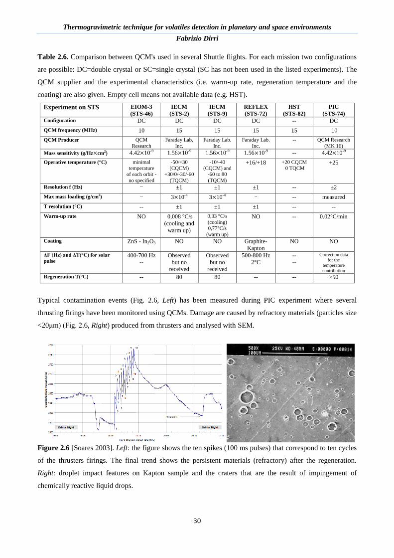
Typical contamination events (Fig. 2.6, Left) has been measured during PIC experiment where several

thrusting firings have been monitored using QCMs. Damage are caused by refractory materials (particles size

<20μm) (Fig. 2.6, Right) produced from thrusters and analysed with SEM.

Figure 2.6 [Soares 2003]. Left: the figure shows the ten spikes (100 ms pulses) that correspond to ten cycles

of the thrusters firings. The final trend shows the persistent materials (refractory) after the regeneration.

Right: droplet impact features on Kapton sample and the craters that are the result of impingement of

chemically reactive liquid drops.


Fabrizio Dirri

31

The QCM for STS are mainly used to monitor contamination and return flux particles on the spacecraft, as

well as to estimate the AO erosion in the upper terrestrial atmosphere. The QCMs used on STS have shown:

in the EIOM-3 experiment the contamination an increase in weight and a mass deposition of 0.2

μg/cm2 in 424 days;

in IECM, a mass deposition of 39 μg/cm2 (X direction), 16.4 μg/cm

2 (-Y direction) 1.6 μg/cm

2 (-X

direction) and 1.2 μg/cm2

(-X and Z directions) in 244 hours;

in the PIC experiment, a deposition of 2.56 μg/cm2 was measured on the Mir Station, 130-N Russian

due to contaminants containing 7.5% of refractory materials and 80% of volatiles sublimating at

52°C; and a mass deposition of 0.384 μg/cm2 was measured by the thrusters firings of the Orbiter

PRCS (only 2% of refractory materials).

By means of SEM analyses, contaminants have been found to have different composition: Carbon and

Silicon particles (EIOM-3); Silicon, Aluminum, Magnesium, Zinc, Sulfur, Titanium and Chlorine (between 1

μm and 2 μm in size for aluminum and up to 370 μm for Zinc particles) (IECM experiment); and thruster

firings particles (PIC).

Table 2.7. Characteristics of QCMs used in satellite mission. Empty cell means not available data. The

crystal configuration can be double crystal (DC) or single crystal (SC) (see chapter 3) and the QCM supplier

are QCM Research, Faraday Laboratory and Meisei Electric.

Satellite Mission SDS-4

(2012)

SMART-2

(2015)

SMART-1

(2003)

MSX

(1996)

Deep

Space1

(1998)

OGO-6

(1969)

MEDET

(2008)

Configuration SC DC DC DC DC DC SC

QCM frequency

(MHz) 9 10 10 10 TQCM

15 CQCM 10 10 10-11

QCM Supplier Meisei Electric Co.

QCM Research

(MK 17)

QCM Research

(MK 17)

QCM Research

(MK 16, MK

10)

QCM Research

(MK 16)

Faraday Lab.

Inc. (Mckeown)

Variation of

commercially

QCM

Mass sensitivity

(g/Hz cm2)

1 ng (T=const)

100 ng (over T

range)

4.4 10-9 4.4 10-9

4.42 10-9

TQCM

1.96 10-9

CQCM

4.43 10-9 3.5 10-9 4.42 10-9

Operative

Temperature(°C) from -40

to+65

from -50 to

120

from -50 to

120

-253 for

CQCM -40/-50 for

TQCM

from -43°C

to +80°C

from -

50°C to

100°C

Temperature

of RAM

direction

Resolution f(Hz) -- 0.1 0.1 ±2 -- ±1 --

Max mass loading

(g/cm2) -- -- -- 3.5 10-6 CQCM

3.3 10-6 TQCM >10-4 10-5 --

T resolution (°C) -- -- -- ±0.25 <±0.2 10-4 --

Warm-up rate

(°C/min) -- -- NO 2.5 -- NO NO

Coating Carbon NO NO NO NO MgFl Carbon

ΔF(Hz) and ΔT(°C)

for solar pulse -- -- -- 300-450

Temperatures

are not

available

<250 Temperatures

are not

available

Decrease of

contamination

due to solar

exposure

--

Regeneration T(°C) 85 -- -- 60 75 100 Present


Fabrizio Dirri

32

In the last case, the image obtained with the SEM showed the damage produced on a small Kapton sample:

small (<4 μm), medium (5-10 μm) and large craters (11-20 μm) in the sample. During these experiments, the

Sun radiation on the crystal surface induced a frequency variation, ascribed to the temperature change. The

frequency variation with temperature is different for the EIOM-3, REFLEX and IECM experiments, and

depends on the crystal coating and on the incidence angle.

QCM’s have been also applied in satellite missions, in order to test and monitoring new technologies aboard

on the spacecraft. QCM’s supplier, characteristics and performances in seven satellite mission of JAXA

(SDS-4), NASA (DS1, MEDET, OGO-6, MSX) and collaborations with ESA (SMART 1 and 2) are

summarized in Tab.2.7. The main goals of QCMs have been:

to estimate the erosion due to AO (MEDET, SDS4);

to measure the contamination from the solar panels of the spacecraft (OGO-6);

to control the contamination induced from the Propulsion System of the spacecraft (DS1);

to monitor the contamination and the degradation near the scientific instruments, i.e. solar cell,

telescope (MSX, SMART1);

to monitor the frequency trend, when the QCMs are exposed to full or partial sunlight (MSX).

In SDS-4 satellite, a frequency increase of 200 Hz was observed in the launch phase, due to the erosion of

coating materials of the QCM surface. In MEDET experiment the carbon-coated QCM showed a frequency

increase of 60 Hz (after two weeks), which indicated a linear decrease of carbon mass, due to AO erosion.

The main contamination sources is often generated by the Solar panels of the spacecraft. OGO-6 experiment

measured a contamination of 10-5

g/cm2 during full exposition to Sun (Solar panels temperature of 72°C) and

9×10-6

g/cm2 during the maximum eclipse (30% in the Earth's shadow and Solar panels temperature of

60°C).The mass loss was due to the fact that the lower flux from the solar panel did not balance the

contaminant desorbed from the crystal surface.

During the launch phase of DS1 mission, QCMs were used to monitor the ion propulsion induced

contamination. A total contaminant mass of 0.8 μg/cm2 has been measured. This mass has been removed

when the DS1 has been rotated to Sun. Otherwise, in MSX experiment, a CQCM placed near the SPIRIT3

telescope revealed oxygen and argon (film thickness deposition of approximately 200 Angstrom), whereas

four TQCM’s placed in different locations measured a total thickness (since launch) of 134, 144, 13, and 63

Angstrom, respectively. In this scenario TQCM’s have the disadvantage of being sensitive to incident solar

flux. The frequency showed a negative shift of 240-450 Hz depending on full or partial exposure to Sun

conditions. The regeneration temperature never exceeded the 100°C (OGO-6) in all the experiments (i.e.


Fabrizio Dirri

33

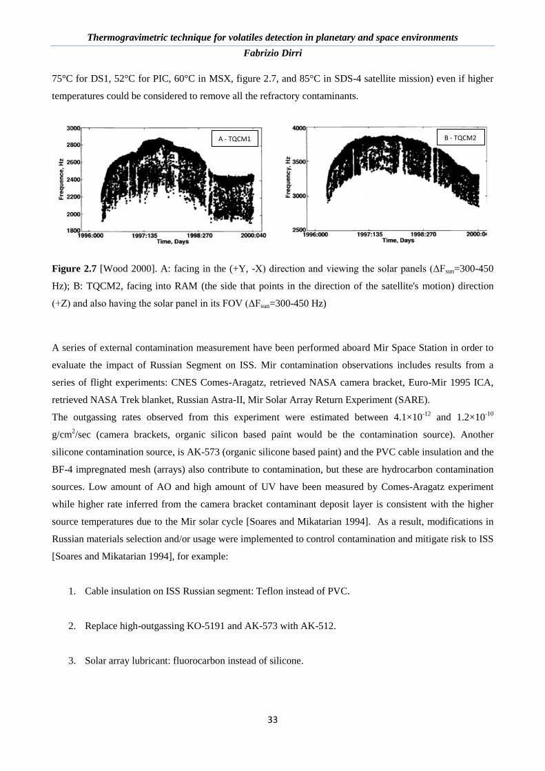
75°C for DS1, 52°C for PIC, 60°C in MSX, figure 2.7, and 85°C in SDS-4 satellite mission) even if higher

temperatures could be considered to remove all the refractory contaminants.

Figure 2.7 [Wood 2000]. A: facing in the (+Y, -X) direction and viewing the solar panels (ΔFsun=300-450

Hz); B: TQCM2, facing into RAM (the side that points in the direction of the satellite's motion) direction

(+Z) and also having the solar panel in its FOV (ΔFsun=300-450 Hz)

A series of external contamination measurement have been performed aboard Mir Space Station in order to

evaluate the impact of Russian Segment on ISS. Mir contamination observations includes results from a

series of flight experiments: CNES Comes-Aragatz, retrieved NASA camera bracket, Euro-Mir 1995 ICA,

retrieved NASA Trek blanket, Russian Astra-II, Mir Solar Array Return Experiment (SARE).

The outgassing rates observed from this experiment were estimated between 4.1×10-12

and 1.2×10-10

g/cm2/sec (camera brackets, organic silicon based paint would be the contamination source). Another

silicone contamination source, is AK-573 (organic silicone based paint) and the PVC cable insulation and the

BF-4 impregnated mesh (arrays) also contribute to contamination, but these are hydrocarbon contamination

sources. Low amount of AO and high amount of UV have been measured by Comes-Aragatz experiment

while higher rate inferred from the camera bracket contaminant deposit layer is consistent with the higher

source temperatures due to the Mir solar cycle [Soares and Mikatarian 1994]. As a result, modifications in

Russian materials selection and/or usage were implemented to control contamination and mitigate risk to ISS

[Soares and Mikatarian 1994], for example:

1. Cable insulation on ISS Russian segment: Teflon instead of PVC.

2. Replace high-outgassing KO-5191 and AK-573 with AK-512.

3. Solar array lubricant: fluorocarbon instead of silicone.

A - TQCM1 B - TQCM2


Fabrizio Dirri

34

2.4. Volatiles reservoirs in planetary bodies detectable by TGA

The chemical and mineralogical analysis on asteroidal and cometary samples will help the classification of

these minor bodies of Solar System (thanks to Sample Return Mission, e.g. Stardust, Hayabusa1 etc.). In

order to know the mineralogical composition of these bodies, a study related to Chondrite meteorites

(asteroids analogues) that are classified in Carbonaceous, Ordinary and Enstatites (which show different

organics content inside, Tab. 2.8) should be done. In particular, the asteroids span very different

mineralogical compositions: some of them appear to be completely unprocessed while other ones are

composed by processed materials. In order to understand the mineralogical history of the processes

concerning asteroids evolution, all the thermodynamical and thermochemical processes should be taken into

account. In particular, the asteroids represent a great opportunity to study a possible cometary-like activity

and to exactly determine the desorption rate and even to discern the refractory/volatile ratio. Mainly, the

thermodynamical processes are related to ejection (sublimation or vaporization) of a mixture of gas or dust.

Gas molecule rates are easily monitored at sublimation temperature at which the process occurs. For

example, the water in space can be collected at T<77 K [Tribble 1996] while for tiny dust particles it is also

important to monitor the ejection speeds.

Table 2.8 [Grady and Wright 2003, Sephton 2002, Schaefer and Fegley Jr. 2006, Stalder and Skogby 2002].

Carbon, organic compounds and water abundance in the three families of chondrites.

Chondrite Class Carbon content Organic content Water content

Carbonaceous 0.1-5 % 0-4% 0-20 %

Ordinary 300-6000 ppm ~ 0.1% ~ 0.3%

Enstatites 1500-7000 ppm - ~ 1000 ppm

On the other hand, the Carbonaceous Chondrites (CC) (related to primitive asteroid, the most

thermodynamically and chemically processed), are divided in groups showing different volatile content (see

Tab.2.9) which can be used as a marker for asteroid types. The CI, CM, CR groups form the first ensemble

with similar organic and water content. The other CC are included in the second ensemble, which is

characterized by very low volatile (water, organic) content.


Fabrizio Dirri

35

Table 2.9 [Grady and Wright 2003, Remusat 2008]. Carbon, organic and water content in carbonaceous

chondrites.

CC Group Carbon content Organic content Water content

CI 2-5 % 1-4 % 18-22 %

CM, CR 2-5 % 1-4 % 2-16 %

CO 0.1-1.1 % < 1 % 0.3-3 %

CV 0.1-1.1 % - 0.3-3 %

CK 0.1-1.1 % - -

CH, CB 0.2-1 % - 0.3-3 %

Table 2.10. Combustion temperatures of Chondrites components.


Fabrizio Dirri

36

Thus, QCM-based device equipped with built-in heater can be used to perform heating cycles up to

400°C on Chondrites samples in order to study the decomposition processes of materials at different

temperatures (Tab. 2.10). The decomposition processes will be:

1. organics degassing between 200°C and 400°C [Grady 2002, Sephton 2002, Halbout 1986];

2. water desorption. A distinguishing between physically adsorbed water (loosely bound molecules

held by Van der Waals’ forces), that desorbs to lower temperatures (up to 160 °C), and surface

bounded water (molecules more tightly bounded, attached to basal clay surfaces), that desorbs at

higher temperatures (above 300°C) have to be done. Surface bounded water can be detached from

organic materials or from phyllosilicates [Bruckenthal and Singer 1987, Halbout 1986];

3. inorganic sulphur compounds, present only in CI chondrites, that desorbs between 200-250 °C

[Halbout 1986];

4. carbonates and nanodiamonds, that are decomposed above 400 °C [Sephton 2002].

From table 2.10 a thermal trend is defined:

T< 160°C (433 K): in this range only physically adsorbed water is released.

200°C (473 K)< T < 300°C (573 K): organic matter decomposition starts at 200 °C and up to 300 °C

is the only compound to be decomposed. If sample composition is similar to CI’s, in addition to the

organic matter we can detect the inorganic sulphur decomposition too, even if its abundance is not

larger than about 12 % of the organic [Halbout 1986].

300°C (573 K)< T < 450°C (723 K): at 300°C even surface bounded water begins to desorbs and

partly is desorbed from organic compounds. In this range, the desorption of both water and organics

is observed.

T>450°C (723 K): neither organics and water evaporate, but only carbonates and nanodiamonds.

TGA can be used to study the thermodynamical processes as well as to detect surface bound water,

carbonates, organics. In particular, QCM can measure [Palomba 2011]:

dust settling rate and ice content: VISTA instrument can operate in accumulation mode revealing

the ice falls by applying a heating cycle few degrees above the water frost point, while the dust

remains onto the crystal. This operation allows also the determination of the water frost temperature

and (knowing the actual pressure) of the atmospheric humidity;

humidity: measurements of water vapor local abundance (Langmuir equation);

physically adsorbed water in the dust heating up to 240 K, the mass difference at the beginning and

at the end of the cycle gives the adsorbed water mass;


Fabrizio Dirri

37

2.5. Dicarboxylic acids

Dicarboxylic acids are organic compounds with a general chemical formula:

where n is the number of carbon atoms. According to IUPAC nomenclature, dicarboxylic acids are named by

adding the suffix dioic-acid to the name of the hydrocarbon with the same number of carbon atoms, e.g.,

nonanedioic acid for n = 7. The dicarboxylic acid contain two carboxylic acid functional groups and are used

to prepare copolymers and polyamides and polyesters [Dirri 2016b].

Dicarboxylic acids the most abundant class between the organic components of PM [Rogge 1993] and are

present in various concentrations in different terrestrial environments, e.g. marine, rural, urban [Kawamura

2005, Yu and Fraser 2004, Limbeck 2001]. Their formation in atmosphere is likely due to photochemical

reactions in gaseous phase involving VOC (in particular aliphatic and aromatic hydrocarbons) of biogenic

and anthropogenic origin. By means of the mass spectrum of atmospheric aerosols, we can considered the

Dicarboxylic acids as "markers" of SOA [Schuetzle 1975]. Typical concentrations of dicarboxylic acids in

ambient air are a few nanograms per cubic meter and thus contribute to a large fraction of the total

identifiable resolved organic mass in fine aerosols [Dirri 2016a].

These compounds play an important role on physical-chemical reactions involving aerosol particles, that

may be gathered in agglomerates (sub-micron sized), and represent an important component of the

atmospheric aerosol particles, both in remote and urban areas [Rohrl and Lammel 2001].

Concentrations of longer-chain diacids (C6–C9) varied in different seasons and size fractions with suberic

acid (C8) being the most abundant in the wet season in PM2.5, adipic acid (C6) and azelaic acid (C9) in the dry

season in PM2.5 and C9 in both seasons in PM10 [Mkoma and Kawamura 2013].

The oxalic acid is the most abundant dicarboxylic acid in the tropospheric aerosol and comprises 41-67

percent of the total diacids [Sorooshian 2006, Kawamura and Keplan 1983] whereas the succinic and

malonic acids are less abundant and reach peaks of 4-8.7 percent during the summer [Kawamura and

Ikushima 1993]. Adipic and succinic acids have been identified in laboratory studies as SOA products

(reaction of O3 and cyclohexene) [Hatakeyama 1985]. The Adipic acid is related to N2O emission, a

greenhouse gas that causes stratospheric ozone depletion [EPA 2016] whereas the succinic acid origins

probably from biogenic sources, and is an important compound in biochemistry due to its role in the citric

acid cycle (Krebs cycle). The azelaic acid is considered a photon-induced oxidation's product, deriving from

biogenic unsaturated fatty acid, presenting one or more double bond in their chain [Kawamura and Keplan,

1983]. Succinic and oxalic acids had been proven to be part of the organic materials that contribute to form

condensation nuclei of atmospheric clouds [Kerminen 2000, Prenni 2001] and it has been suggested that the

ratio between oxalic and succinic acid is a good marker of the atmospheric aerosol oxidation state


Fabrizio Dirri

38

[Kawamura and Ikushima 1993]. On the other hand, adipic-azelaic ratio could be an indicator of

anthropogenic sources, considering that adipic acid derives from cycle-hexane's oxidation [Dirri 2016a].

Dicarboxylic acids have been found also in carbonaceous chondrites [Andersen 2005, Briscoe 1993],

meteorites associated to the primitive asteroids; and hence could give information about chemical and

mineralogical composition of the early Solar System. Chemical analyses on carbonaceous chondrites

revealed a variety of organic compounds, including amino acids, aliphatic and aromatic hydrocarbons,

mono-carboxylic acids and some dicarboxylic acids, such as succinic acid and adipic acid in small quantities

(5.9 µg/g and 0.7 µg/g, respectively). In this scenario, the presence of the succinic acid is consistent with a

synthesis from hydrogen cyanide and ammonia. In particular the succinic acid/β-Alanine (amino acid) ratio

makes it possible to estimate the relative period of synthesis of organic compounds on the Murchison

meteorite parent body [Peltzer 1984].

Carboxylic acids have been found in water samples (i.e. indoor contamination) acquired during few STS

missions. In particular, the chemical constituent includes contaminants released into the cabin air, come from

crew activities, such as by product of metabolism, food preparation and hygiene activities (including the use

of cleaners and disinfectants); from revitalization system and from hardware off-gassing, from payload

experiments. In this way, the humidity condensate is an important source of indoor water contamination (and

probably most variable) and collected by the cabin heat exchanger, which is controlled by the spacecraft's air

revitalization system. Different samples have been collected during the STS missions and many organic

compounds were identified including: alcohols, amines, carboxylic acids, ethers, esters, ketones, phenols and

thiourea. In 1991 and 1992, samples were collected from STS-40, STS-42, STS-47 and STS-50 even if the

long delay after landing until samples could be collected could affected their chemical composition [National

Research Council 2000]. Besides, the assessment of atmospheric quality aboard Shuttle mission have

revealed the presence of organic compounds that appeared in the humidity condensate. Additional samples

have been collected from STS-68 and from Mir station [James 1994].

Thus, assuming the carboxylic acids implication in the humidity condensate aboard STS mission and Mir

Station, a characterization of these compound and specifically of dicarboxylic acids would be useful for

samples analysis on ground, to understand the toxicity level of these compounds in the STS internal

atmosphere.

2.5.1. Physical properties

Organic compounds are characterized by molecular lattice whose molecules are arranged to form crystals.

The thermal reactions of organic compounds in the solid state depend on their interatomic relations and

cohesive forces acting between their crystals [Muraishi and Suzuki 1994]. Generally, dicarboxylic acid

which are originate from combustion of fossil fuels [Kawamura and Kaplan 1983] and biomass burning

https://www.google.it/search?hl=it&tbo=p&tbm=bks&q=inauthor:%22National+Research+Council%22



Fabrizio Dirri

39

[Narukawa 1999] are subjected to thermal breakdown of crystalline organic compounds, which is both a

physical and chemical process [Muraishi and Suzuki 1994].

Dicarboxylic acids are colorless, odorless crystalline substances at standard conditions. In table 2.11 are

listed the major physical properties of some saturated aliphatic dicarboxylic acids with carbon number from

2 to 10 atoms [Rozaini 2012]. As shown, the acids density decrease steadily with increasing chain length

whereas melting point and water solubility show an alternate order: acids with an even number of carbon

atoms have higher melting points than the next higher odd-numbered dicarboxylic acid [Rozaini 2012]. The

water solubility is higher for odd-numbered C atoms and lower for even-numbered C atoms.

In the range: n = 6 – 10, dicarboxylic acids show a lower solubility than those in the range: n = 2 – 5. As

chain length increases, the influence of the hydrophilic carboxyl groups diminishes; from n = 5 (pimelic

acid) onward, solubility in water decreases rapidly.

Table 2.11 [Rozaini 2012]. Physical characteristic of dicarboxylic acids. The bold acid names are those

analysed in this work.

IUPAC name Acid name C Chemical Structure Molecular

weight (g/mol)

Density at

25°C (g/cm3)

Solubility

(mol/kg)

Boiling point Melting

point

Ethanedioic Oxalic 2

90.03 1.653 1.131 - 189.5

Propanedioc Malonic 3

104.06 1.619 16.03 - 135

Butanedioic Succinic 4

118.08 1.572 0.748 235 188

Pentanedioic Glutaric 5

132.11 1.424 8.468 200 99

Hexanedioic Adipic 6

146.14 1.360 0.171 265 153

Heptanedioic Pimelic 7

160.17 1.329 0.423 272 106

Octanedioic Suberic 8

174.19 1.266 0.0139 279 144

Nonanedioic Azelaic 9

188.22 1.225 0.00946 287 108

Decanedioic Sebacic 10

202.25 1.207 0.00012 - 134.5


Fabrizio Dirri

40

2.5.2. Chemical properties

The chemical behavior of dicarboxylic acids is determined by their function groups, e.g. the carbonyl or

hydroxyl group. Certain chemical reactions of dicarboxylic acids lead to unusual results as compared with

those of monocarboxylic acids because there are two carboxyl groups in each molecule [Muraishi and Suzuki

1994].

Thermal decomposition of dicarboxylic acids gives different products depending on the chain length, i.e.

acids with an even number of carbon atoms require higher decarboxylation temperatures than the next higher

odd-numbered homologues; lower dicarboxylic acids decompose more easily than higher ones. With the

exception of oxalic acid, dicarboxylic acids are resistant to oxidation. Furthermore, the thermal behavior of

malonic acid and sebacic acid (dicarboxylic acids), may be expected to differ from formic and acetic acid

(monocarboxylic acids), because of the separation of the two carboxylic acid groups by CH, which reduces

the spatial restriction in bonding [Rozaini, 2012]. The main thermal and chemical properties of dicarboxylic

acid are summarized as follow:

Oxalic acid: heating this compound above 190 °C, a decompositions to carbon monoxide, carbon

dioxide, and water occurs.

Malonic acid: at temperatures above 150°C, this compound is decarboxylated to acetic acid

HOOC-(CH2)n-COOH-CH3COOH + CO2. When malonic acid is heated in the presence of P2O5 at

150 °C, small amounts of carbon suboxide (C3O2) are also formed.

Succinic and glutaric acid: it is possible to have cyclic anhydrides on heating (Fig. 2.8). Besides,

when the ammonium salt is distilled rapidly from succinic, succinimide is formed, with the release of

water and ammonia.

Figure 2.8 [Rozaini, 2012]. Succinic and glutaric acids are converted into cyclic anhydrides on heating.

Adipic, Pimelic and Suberic acids (n from 4 to 6): a split off carbon dioxide and water to form

cyclic ketones has been possible, i.e. HOOC-(CH2)n-COOH (CH2)n C=O+CO2+H2O.


Fabrizio Dirri

41

Azelaic acid: heating this compound at P standard, starts to decay at 360°C.

Dicarboxylic acids are mainly used as intermediates in the manufacture of esters and polyamides. Esters

derived from monofunctional alcohols serve as plasticizers or lubricants. Polyesters are obtained by reaction

with dialcohols. In addition, dicarboxylic acids are employed in the manufacture of hydraulic fluids,

agricultural chemicals, pharmaceuticals, dyes, complex agents for heavy-metal salts, and lubricant additives

(as metal salts) [Rozaini, 2012].

2.5.3. Bio-markers compounds

The dicarboxylic acid are an important group of Water-Soluble Organic Compounds (WSOC) in the

atmospheric aerosols [Kawamura and Ikushima 1993, Rogge 1993]. Because of the low vapor pressures and

high water solubility, these compounds have received much attention due of their potential roles in affecting

the global climate.

The most abundant is oxalic acid followed by malonic and succinic [Kerminen 2000]. The percentage of

diacids content is about 1-3% of the total particulate carbon in the urban areas and even above 10 % in the

remote marine environment [Kawamura and Ikushima 1993, Kerminen 2000]. In particular, the

concentration ratios of these diacids of linear sequence, i.e. C3/C4 and C6/C9 mass ratio, help to know the

ratio between anthropogenic and biogenic source and their precursors in the atmosphere [Kawamura and

Ikushima 1993, Ho 2006, Ray and McDow 2005]. It has been suggested that the ratio C3/C4 from vehicular

emission (0.25-0.44 in urban aerosol and lager than unity for rural aerosols) [Kawamura 1996] could provide

the oxidation signature of anthropogenic aerosols because of the succinic acid, after several photochemical

processes, can be the precursor element of malonic and oxalic acids. On the other hand, because of the

azelaic acid and adipic acid have been proposed as one of the reaction products of ozonolysis of biogenic

unsaturated fatty acids [Kawamura and Keplan 1983] and the product of anthropogenic cyclohexene

respectively [Kawamura and Ikushima 1993], the ratio C6/C9 could be used as an indicator of biogenic

sources.

In this work, five dicarboxylic acids with lower molecular weight (C number from 2 to 9) are analysed,

founding the thermodynamical properties described in chapter 3. In figure 2.9 are shown the chemical

structure of these compounds.


Fabrizio Dirri

42

Figure 2.9 [PubChem database, 2016]. Chemical structure of C2 to C10 dicarboxylic acids are shown. Red

and gray atoms are the oxygen and carbon respectively while the light blue atoms are hydrogens.


Fabrizio Dirri

43


Fabrizio Dirri

44

Chapter 3. Thermo-physics and Thermogravimetry: basic concept

3.1. Introduction

The chemical-physical and thermodynamic properties of materials/compounds (i.e. vapor pressure, enthalpy,

entropy and Gibbs free energy) are fundamental to know their behaviour in different environment (e.g.

terrestrial atmosphere, space etc.) with different external conditions, i.e. pressure and temperature. Thus,

thermochemical relations, i.e. Clausius-Clapeyron, Langmuir and Van't Hoff equation and physical-chemical

quantities for organic compounds characterization are introduced as well as the thermodynamic quantity as

vapor pressure and the enthalpy of phase change which help to identify a compound.

The basic concept of Thermogravimetric Analysis (TGA) and the working principle of microbalance are

explained. The Quartz Crystal Microbalance (QCM), Sauerbrey equation and the applications QCM-TGA

are discussed in preparation to experimental procedure and results explained in chapters 5-6.

Finally, VISTA instrument (QCM-based device) and the two sensor heads, i.e. Sensor Head 1 (SH1) and

Sensor Head 2 (SH2) breadboards are introduced and explained in depth considering all the sub-system

units. The Engineering Model of SH1 is also explained. Furthermore, the main innovations, the measurement

capability and the scientific goals of SH1 and SH2 are described.

3.2. Thermochemical processes

3.2.1. Phase change thermodynamic processes

The matter phases are class of various molecular motions existed at particular temperatures: at low

temperatures, the molecular motion is restricted so that molecules are bounded with strong intermolecular

forces while at high temperatures, the molecular motion is due to the translational energy of molecules (the

intermolecular forces are ignored). At intermediate temperatures, molecules are in translation mode and

bounded with each other.

According to the intermolecular forces between molecules, the matter phases are classified into three

different aggregation states: solid, liquid and gas and in rare case, plasma. In order to change the aggregation

state it is necessary to change the intensity of the cohesion force between molecules, i.e. varying the kinetic

energy. In fact, a thermodynamic phase change is followed by heat variation between compound and external

environment. Generally, when heats is provided a liquid or gaseous states are promoted (the molecules are

less bounded). On the other hand, if heats is subtracted the inverse phase change is promoted [Levine 1978].

Basically, the thermodynamical phases show a difference in molecules kinetic energy: the solid to liquid

change takes place at the melting point of solid while the liquid to gas change is takes place at boiling point.

Conversely, if pressure increase, the vapor phase to liquid phase change and liquid to solid state phase

changing are promoted. If pressure decrease, the inverse phase change is facilitated. The transitions between

the solid, liquid and gaseous phase of a single component, due to the effects of temperature and/or pressure


Fabrizio Dirri

45

are: solidification (liquid to solid), sublimation (solid to vapor), deposition (vapor to solid), condensation

(vapor to liquid) and evaporation/boiling (liquid to vapor).

3.2.2. Activation energy, vapor pressures and enthalpy of phase change

A compound can be characterized by identifying its thermodynamical properties. For example, the

knowledge of pure component vapor pressures is essential for calculations of gas/particle partitioning of

compounds forming terrestrial atmospheric aerosols [Booth 2009] as well as the knowing of the enthalpy and

entropy of sublimation which is different for each compound [Dirri 2016a].

A chemical-physical process happens when the molecules (with a correct orientations) velocity is high

enough so that kinetic energy of collision is higher than the minimum energy barrier. The activation energy

is the minimum required energy to have collisions: Ea is measured in kilojoules per mole (kJ/mol). During a

chemical reaction, if the kinetic energy is higher than the minimum energy it is possible to have the new

products formation. Different Ea values are shown in figure 3.1.

Figure 3.1. Activation energy for exothermic and endothermic reactions. The maximum energy point is

called "transition state" which representing a chemical transitory species (due to the energy levels which are

higher than products and reagents).

Thus, the activation energy, i.e. Ea (kJ/mole) is connected to the temperature T(K) and rate constant k by

means of the Arrhenius equation:


Fabrizio Dirri

46

(3.1)

where A=const, proportional to the collision frequency and expressed as (1/s) and R, the gas constant (kJ

mol-1

K-1

). Ea can be retrieved by plotting ln(k) vs. 1/T. The slope of the straight line obtained will equal to -

Ea /R. Generally, the most of chemical reaction show Ea values between 40 and 150 kJ/mol while at Tamb up

to 80 kJ/mol the reaction proceed quickly.

Enthalpy is a typical thermodynamic quantity that can used to characterizes the organic compounds;

specifically the enthalpy of sublimation. When thermodynamic process occurs at constant pressure, the heat

evolved in thermochemical process (either released or absorbed) is equal to change in enthalpy. Enthalpy (H)

is the sum of the internal energy (U) and the product of pressure and volume (PV):

(3.2)

Enthalpy is a state function which depends entirely on the state functions T, P and U. It is possible to express

the enthalpy as change in enthalpy (ΔH) between initial and final states:

(3.3)

considering constant pressure the heat flow (q) for the process is equal to the change in enthalpy:

(3.4)

ΔH and q relationship can be determined by looking exothermic or endothermic reactions. If the heat is

absorbed the reaction will be endothermic (the heat from the surrounding environment is consumed: q>0). At

constant temperature and pressure, with q>0, ΔH is also positive. If the heat is released the reaction will be

exothermic (the heat is emitted to surrounding environment: q<0). If q<0, ΔH will be also negative [Atkins

and de Paula 2006]. The enthalpy can be represented at the standard state (P=1 bar) as ΔHo, which is the

enthalpy of a phase transition (e.g. ice to liquid water) that require or absorb a particular amount of standard

enthalpy:

Standard enthalpy of vaporization (ΔHo, vap) is the energy that must be supplied as heat at constant

pressure per mole for vaporization (liquid to gas).


Fabrizio Dirri

47

Standard enthalpy of fusion (ΔHo, fus) is the energy that must be supplied as heat at constant pressure

per mole of molecules for melting (solid to liquid).

Standard enthalpy of sublimation (ΔHo, sub) is the energy that must be supplied as heat at constant

pressure per mole for sublimation.

Considering the Hess law, in a chemical reaction the thermal effects (at P=const) depends only to initial and

final state of the system. Thus, the enthalpy variation can be calculated by means of the sum of different

partial enthalpies:

(3.5)

i.e. for sublimation process, the final enthalpy is the sum of the enthalpy of fusion and vaporization.

Applying different thermal cycles to compounds it is possible to calculate the enthalpy of vaporization and

the enthalpy of fusion each one, verifying that the difference is the enthalpy of fusion [Price 2001]. In

particular, it can be assumed that enthalpy of condensation is the reverse of the enthalpy of vaporization and

the enthalpy of freezing is the reverse of the enthalpy of fusion. The enthalpy variation of complete process

is the sum of the enthalpy changes for each of the phase transitions [Petrucci 2007].

In this work, different sublimation processes have been monitored (at P=10-6

mbar) and the enthalpy of

sublimation, i.e. the enthalpy change accompanying the conversion to one mole of solid substance directly

into vapor phase at a given temperature [Tyagi 2006], has been inferred for five different crystalline pure

organic compounds. The enthalpy of sublimation can be also inferred by means of Clausius-Clapeyron

equation that characterizes a phase transition. The vapor pressure can be obtained at each temperature Ti and

the enthalpy variation from vapor pressure at two different temperatures:

(3.6)

being ΔH the specific latent heat of the process (sublimation, vaporization, or fusion), p the vapor pressure

and ΔV the difference between volumes of gaseous and solid/liquid (sublimation/vaporization) phase,

respectively. If the products are in gaseous phase and at temperatures much smaller than their critical one,

they can be approximated as ideal gases, i.e. ΔV~ Vgas=RT/p. Replacing in the equation 3.6, we have the

differential form:


Fabrizio Dirri

48

(3.7)

In order to characterize a pure substance, the thermogravimetry can be used to determine the vapor pressure,

by recurring at Langmuir equation for free kinetic sublimation/evaporation in vacuum [Langmuir 1913]:

(3.8)

where p is the vapor pressure of the gas, dm/dt is mass loss rate per unit area (the area of the PCM's

electrode) is the deposition rate experimentally measured, Mi the molecular weight, R the gas constant, T the

absolute temperature and α the vaporization coefficient, assumed to be 1 in vacuum environment (Price

2001). Replacing eq. (3.7) in eq. (3.8), it is possible to obtain the enthalpy of sublimation (multiplied by a

constant) as slope of the curve ln(dm/dt)T1/2

versus T-1

(3.9)

where C is the term (2πR/αMi)1/2

that remains constant during all the measurement. The enthalpy of

sublimation/evaporation can be also obtained by means of the Van’t Hoff equation [Benson 1968],

i.e. by measuring at two different temperatures T1 and T2 and the respective rate constants k1 and k2

(the deposition rates on the PCM):

(3.10)

Then, the Van’t Hoff equation (eq. 3.10) can be used to monitor the enthalpy variation in a

temperature range in order to monitor the state functions (e.g. enthalpy, Gibbs energy, and entropy)


Fabrizio Dirri

49

in a transition phase [Dirri 2016a]. According to this relation, for an endothermic process (i.e.

T1>T2 and ΔH>0): k1>k2, i.e. the temperature is directly proportional to rate constant.

3.2.3. Entropy and Gibbs free energy: spontaneous and non-spontaneous reactions

Generally, the thermodynamic quantity called entropy (S) measures the degree of the disorder of the system.

The entropy of system increases as the disorder of the system also increase. This thermodynamic parameter

is a state function such that is possible to define the entropy variation as the difference between the initial

and final states:

(3.11)

The entropy variation for fusion process will be: ΔS>0 because the disorder degree increase.

Entropy can be transferred in two forms: heat transfer (to a system) and mass flow (from a system).

If the thermodynamic process happens at equilibrium conditions (reversible), the ratio of the heat

transfer Q/T (absolute temperature) is called entropy flow or entropy transfer:

(3.12)

Since T(K) is always positive, the direction of the entropy transferred is the same of the heat transfer

direction. Defining the entropy as heat of reaction, if the heat transfer between two phase is

reversible and the process are on equilibrium at temperature: Ttrasf, we can define

while ΔS is given to:

(3.13)

Thus, we can have three different scenario:

If ∆S system > 0, then the system is at equilibrium.

If ∆S system = 0, the system is at equilibrium.

If ∆S system < 0, then the reverse process is spontaneous.

In order to determine spontaneity, it would be better to have a function depending to the system only, i.e. the

Gibbs free energy (G). This is a thermodynamic quantity that can be used to retrieve the maximum work


Fabrizio Dirri

50

performed by a thermodynamic system at a constant temperature and pressure (isothermal, isobaric). The

Gibbs free energy is defined as:

(3.14)

Because of H, S, T are state functions as well as G, for thermodynamic process (initial to final stage) it is

possible to define the Gibbs free energy as ΔG in order to determine the spontaneity of chemical reaction at

T, P= const. In these conditions, ΔG can be rewritten as:

(3.15)

ΔG is mainly composed by two contributions: energetic, i.e. ΔH and entropic, i.e. TΔS. The exothermic

reactions are facilitated (ΔG<0) with ΔH<0 (Fig. 3.2, Left) and a positive entropy variation (ΔS>0).

Generally, ΔH contribution is higher than ΔS thus, the sign of ΔG is determines by ΔH. When ΔH

contribution is small, TΔS can determine the ΔG sign: the endothermic reaction can occurs spontaneously if

The quantity TΔS became more important in this reaction when the temperature increase. During a fusion

processes (evaporation and sublimation): Δ > 0 e Δ > 0, which means that when the temperature

increase, also TΔ increases while for T > we have Δ < 0 (the fusion process in spontaneous).

Figure 3.2. Left: Gibbs-Helmholtz plot for an endothermic reactions. Right: Gibbs-Helmholtz plot for an

exothermic reactions.


Fabrizio Dirri

51

For exothermic reactions, the slope for the Gibbs equation is negative (Fig. 3.2, Left). When the temperature

increases the Gibbs free energy variation increases: Tfinal< Tinitial , ΔGfinal> ΔGinitial.

Instead, for endothermic reactions the slope of the Gibbs equation (Fig. 3.2, Right) is positive. Thus, when

the temperature increases the Gibbs free energy change decreases: if Tfinal> Tinitial , ΔGfinal< ΔGinitial. When

Gibbs free energy variation is negative at Tinitial (spontaneous process), increasing the temperature further

decreases the Gibbs free energy variation (ΔG).

From equation (3.15) it is simple to verify the reaction spontaneity related to ΔH and ΔS signs. Being T

positive, the following criteria of spontaneity is adopted:

considering P,T = const., the different reactions are provided:

ΔH<0 e ΔS>0 always spontaneous

ΔH<0 e ΔS<0 spontaneous if TΔS<ΔH or TΔS>ΔH

ΔH>0 e ΔS>0 spontaneous if TΔS<ΔH

ΔH>0 e ΔS<0 never spontaneous

3.2.4. Enthalpy and Entropy of sublimation from Gibbs free energy

The enthalpy of sublimation can be also obtained combined the Gibbs free energy equation (3.16) which

include the quantities: ΔG and ln(k), where k is defined as the reaction rate:

(3.16)

and the ΔG vs. T dependence:

(3.17)

which gives the final expression as:


Fabrizio Dirri

52

(3.18)

In this case the A constant is: ΔS/R which can be obtained plotting ln of the constant rate with 1/T. From the

slope of the curve it is possible to obtain: ΔH/R, while the quantity ΔS/R can be obtained by the intercept (ΔS

is the entropy of thermodynamic process). Generally, the reaction rates "k" is assumed as the

sublimation/condensation rates from/on specific surface (i.e. PCM surface in this work). In this way,

obtaining the deposition rates of compound it is possible to determine the entropy and enthalpy variation in a

temperatures range. Gibbs free energy can be also obtained in order to know the spontaneity or not of the

reaction. In particular, the phase change from solid to liquid and liquid to solid are characterized by an

increase of disorder: for solid-gas transition (sublimation) ΔS increases, i.e. ΔS>0 e ΔH>0 (endothermic

process).

3.3. Thermogravimetry: basic concept

Thermogravimetry (TG) or Thermogravimetric Analysis (TGA) is a technique used in research and

development of various compounds and materials in order to obtain information about thermal stability and

composition and to monitor different processes, e.g. thermal processes namely sublimation, desorption or

frosting etc. TGA technique measures the amount and change in weight rate of material as a function of

temperature or time in a controlled environment (vacuum, air etc.). The TGA analysis has been frequently

used to monitor the deposition/sublimation and absorption/desorption processes of volatiles compounds in

different environments: outgassing rates from degassing in space [Wood 1996], dehydration and organics

decomposition in minerals [Serpaggi 1999] and the fate of various materials in atmospheric environments

[Elder 1997]. These kind of measurements are used to determine the composition of materials (volatiles and

refractory materials can be distinguished) and to predict their thermal stability at temperatures up to 1000-

1600°C [Sundberg 2004, ELTRA 2016]. By means of TGA, the following processes can be monitored:

Thermal Stability

Oxidative Stability

Composition of Multi-component systems

Estimated Lifetime of a product

Decomposition Kinetics

The Effect of Reactive or Corrosive Atmospheres on materials

Moisture and Volatiles Content

The materials can be characterize by means of the weight loss and weight gain giving several information

about kinetic processes. Considering the weight loss the following processes can be examine in depth:


Fabrizio Dirri

53

1. Decomposition: breaking apart of chemical bonds

2. Evaporation: loss of volatiles with elevated temperature with their evaporation rates

3. Reduction: interaction of sample to a reducing atmosphere (hydrogen, ammonia, etc)

4. Desorption: volatiles or low-volatiles desorption rates

On the other hand, with the weight gain it is possible to study:

1. Oxidation: interaction of sample with an oxidizing atmosphere

2. Absorption: VOC molecules adsorbed

3. Deposition: VOC molecules condensed on a cooled surface

The change in mass measurement can be obtained with a frequency change in time of a microbalance system

while a heating of the microbalance itself (with an integrated heater which allow to control the sample

temperature within 0.1°C) allows to have the desorbed volatiles from deposited sample. Therefore, the

sample is heated and simultaneously weighted and cooled with different thermal cycles. Arranging the

microbalance and the sample in a specific environment (vacuum chamber, laboratory etc.), the temperature

and pressure can be controlled by a separate system. TGA is often coupled with other analytical techniques

as mass spectroscopy in order to obtain the molecular composition of loss volatiles from mineral [Grady and

Wright 2003, Fermo 2006].

In figure 3.3 are shown two typical processes monitored with QCM: desorption and sublimation processes.

In this study, several organic acids have been characterized using microbalance sensor equipped with an

integrated heater in order to study the deposition and desorption processes.

Figure 3.3. Organic material heating by means of microbalance built-in heater. The lighter material is able to

sublime from crystal's surface whereas the refractory material (heavier) stand on microbalance surface. By

means of frequency variation the mass change can be inferred.


Fabrizio Dirri

54

3.3.1. Introduction to transduction mass sensors

The Quartz (SiO2) is the second abundant mineral in the Earth crust and main constituent of magmatic and

sedimentary rocks. In 1880, Jacques and Pierre Curie discovered that a mechanical deformation applied on

some crystals, e.g. Tourmaline and Quartz, were able to determine an electric polarization, proportional to

the applied deformation. This phenomena, i.e. the "direct piezoelectricity" effect which produces a shift of

the electric charges when a mechanical stress is applied. Conversely, the "inverse piezoelectricity" effect,

produces a mechanical deformation when an electric field is applied. The crystal which not show a centre of

symmetry is able to take advantage from this effect. In dielectric materials (crystals, ceramics, polymers)

without centre of symmetry, electric polarization can be generated by a mechanical stress application. The

main important piezoelectric materials are listed below:

Ceramics: Pb (ZrTi), O3 (PZT), PbTiO3 (PT), etc.

Single crystals: Quartz, LiTaO3, LiNbO3, PZN-PT,etc

Polymers: PVDF and copolymers, nylon, etc.

Composites: PZT-polymer 0-3, 2-2, 1-3 composites, etc.

Thin/thick films: PZT, PT, ZnO and AlN films

Quartz Crystal Microbalance (QCM) and Surface Acoustic Wave (SAW) sensors and chemically reactive

materials have been realized using piezoelectric transductors. When piezoelectric device are used as sensors,

it is possible to monitor the frequency and temperature for a thermochemical process by means of oscillator

circuit. QCM is often used as device for mass monitoring thanks to small film deposition on electrode area

which cause the variation of several characteristics of the sensors, i.e. the frequency. Thus, the electric

magnitude monitored is the resonant frequency due to interaction between environmental molecules and the

sensor. The microbalance is useful to monitor the deposition rates of thin films and the affinity between

some fundamental molecules (as proteins) with a specific functionality surfaces (which helps their

identification) in vacuum environment and liquid environment respectively.

3.3.2. Microbalance working principle QCM is able to take advantage of piezoelectric effect thanks to the different SiO2 cut which make it the most

material used in this Sensoristic field. The crystal is composed by two different atomic species connected to

ionic bonds. At equilibrium phase, the barycenter of positive and negative charges is coincident while when

an external force is applied, the barycenter charges is unbalanced and a crystal deformation is obtained. The

consequence will be a moment of dipole which polarize the external surface of the crystal. Thus, in the

piezoelectric effect the electrical and mechanical deformations are completely connected.


Fabrizio Dirri

55

Quartz Crystal Microbalance (or TSMR: Thickness Shear Mode Resonator, 0.8 - 40 MHz) has been the first

piezoelectric device used for chemical reaction processes monitoring in biomedical and industries fields as

well as for environmental applications where the mass, density, viscosity change in time were required. The

QCMs are also used to monitor the absorption/desorption processes and materials corrosion. The

piezoelectric crystal bends in different ways at different frequencies. This bending are called: vibration

modes. The crystal can be assembled in different shapes to achieve different vibration modes. Several modes

have been developed to operate over several frequency ranges: from low kHz range up to the MHz range.

Figure 3.4 shows the vibration modes and the frequencies over which they can work.

Figure 3.4. The possible Vibration Modes with Piezoelectric Ceramics. In particular, the QCM used here are

Thickness Shear Mode Resonator type.

These sensors are composed by AT cut quartz plate (the material deformation act as scrolling of parallel

planes) and metal foil (gold, chrome, platinum) whose goal is to spread out the acoustic wave generated by

electrodes polarization (Fig. 3.5). Thus, the aim of the quartz is to convert the electric power provided by

metal transduction into acoustic waves which are the material reticular vibrations. The generated acoustic


Fabrizio Dirri

56

waves are in transverse mode with a perpendicular propagation on the surface. Thus, the particles movement

is parallel to the surface (Fig. 3.6). Considering the AT cut quartz crystal, the even (n) vibration mode which

satisfy the relation are:

(3.19)

where is the wave velocity in quartz plate (which is 3320 m/s for AT cut) while l is the plate thickness and

n the harmonic order.

Figure 3.5. Quartz Crystal Microbalance (from TamaDevice, Solution and Development). In particular,

quartz plate (transparent surface) and electrode (gold area) are shown. The crystal is supported by two metal

clips.

AT cut

Quartz

Crystal Gold electrode

Metal clip


Fabrizio Dirri

57

Figure 3.6. Waves propagation in QCM. The acoustic waves generated are transversal while their

propagation is perpendicular to the surface.

The most important parameter is "l": the thickness of the crystal. In fact, varying "l" it is possible to have

different resonant frequency of the crystal.

In order to perform TGA measurement, microbalance can be also provided by (integrated or external) heater

and temperature sensor (a thermistor) (Fig. 3.7). The heater and the thermistor allow to monitor the

desorption process of deposited material on the sensor, i.e. temperatures up to 200-250°C can be reached

with thermal cycles to analyze the volatiles substance. In this case, the organic molecular bonds may break or

leak and the desorption material can be quantify by means of the mass variation provided by the sensor.

Figure 3.7. The areal temperature distribution results on QCM equipped with integrated built-in heater from

thermal simulations. In the present design the heater and thermistor are placed onto the QCM opposite faces.


Fabrizio Dirri

58

Figure 3.7 shows a thermal cycle that comes from thermal simulation results for a voltage of 1V, I=50 mA

and a power of 50 mW in air. The experimental tests have been shown as the material deposited on blue

areas is exposed to unvarying temperature. The temperature difference between built-in heater and built-in

thermistor (blue and red areas) is about 10°C.

The microbalance system are sensors able to measure mass variation, Δm, from frequency variation, Δf, using

AT cut crystals which vibrates transversely in the cut orthogonal direction. The propagation of the transverse

acoustic wave happen through the crystal thickness: the waves are back reflected to crystal separation area.

When a sensitive material is deposited on the quartz surface (e.g. gold), the wave will cross the interface

(between the quartz and layer) propagating itself over the layer. Considering the same quartz properties for

this deposited material, a thickness variation ("l" parameter) have to be considered. Taking into account the

equation (3.1), it is possible to obtain the variation in the frequency, Δf, due to the thickness variation of the

crystal, Δl:

(3.20)

the quartz mass is connected to the thickness:

m=ρAl (3.21)

where ρ is the density (2.65 ) while A is the quartz area. By replacing the mass variation to thickness

variation in the expression (3.20)

(3.22)

Using the equation (3.19), the frequency variation can be calculated, obtaining the Sauerbrey equation:

(3.23)


Fabrizio Dirri

59

where is the propagation velocity of the acoustic wave of AT cut resonator while "f" is defined as

fundamental resonant frequency of QCM before layer deposition. In this case, is the sensibility or

Sauerbrey constant (a function of fundamental frequency square) which allow to connect linearly Δf with

Δm. In particular, QCM sensibility is defined as the ratio between the frequency variation and deposited

mass:

(3.24)

From eq. 3.24 it is possible to state that sensor sensibility will be higher reducing the electrode area and

increasing the resonant frequency. The deposited mass will be detected the on electrode surface whereas the

deposited mass outside the electrode will be not revealed. For these reasons, 3D distribution of the electrode

mass sensibility is close to be a Gaussian curve as verified by Sauerbrey: it is maximum in the center and

minimum at electrode boundaries. In figure 3.8, QCM mass distribution is shown. The eq. 3.24 is efficient

for volatiles condensation on crystal surface. Indeed, assuming the deposited molecules as a film which

vibrates at the same quartz resonant frequency, it is possible to consider these molecules as an additional

substrate of crystal layer.

On the other hand, a solid grain (refractory particles) won't be completely integrated with the crystal' surface

and will have a few contact points. These characteristics confirm the importance of this sensor to study the

microscopic processes.

Figure 3.8. QCM sensibility distribution. This distribution is similar to Gaussian curve.


Fabrizio Dirri

60

The quality factor (Q) provides information about the quartz resonator quality and is useful to compare the

different piezoelectric materials. This parameter represent the ratio between the collected energy and

dissipated energy: the value is high into quartz resonator (104

- 105). The product Q-f depends on material

constant:

(3.25)

This relation provides an upper limit for Q which does not reach this value due to crystal defections (related

to the impurity and production process). In table 3.1 the sensibilities of quartz resonators (which depends to

the crystal frequency) are listed (from 1 to 25 MHz).

Table 3.1. QCM sensibilities for difference resonant frequencies.

QCM resonant

frequency (MHz)

Sensitivity

(Hz g-1

cm-2

)

1 2.26×106

2 9.05×106

5 5.66×107

10 2.26×108

15 5.09×108

20 9.05×108

25 1.41×109

3.3.3. QCM and TGA application

In order to characterized a compound and to predict the impact of contamination on spacecraft and satellites

(described in Par. 2.3), QCMs system can be used to obtain information about the temperature-dependent

material and outgassing-deposition kinetics data. Generally, QCMs are usually used to measure the

deposition rates of molecular species on a surface [Garrett 1994, Albyn, 2004] or to obtain typical

thermodynamic properties of VOC's [Dirri 2016a, Freedman 2008]. The official method used for

contamination monitoring is ASTM-E 1559 standard [Garrett 1994] for measuring outgassing and deposition

kinetics by means of temperature-controlled source. The source term, which is representative of the


Fabrizio Dirri

61

material’s outgassing rate, can be used as input for computer programs that predict the rate of deposition of

the emitted or outgassed material on another surface [Albyn 2004]. In ASTM-E 1559, the outgassing process

is controlled by means of two polished QCMs with a sensitivity of at least 10-8

g/cm2 Hz at 25°C with a

natural frequency of 10-15 MHz. The QCMs are angled at 10° for the vertical so their axes intersect at a

point 150 mm from the crystal surface. This intersection point is where the effusion cell orifice exit plane is

positioned. QCMs are cooled at T 193 °C by means of liquid nitrogen reservoir while the effusion cell (a

cylindrical container 65±5 mm) is heated from 25 to 125°C with a precision of ±0.5°C or better. The cell

orifice is at 150±1 mm from the surface of the sensing crystals [Garrett 1994].

In this work, a PCM provided by PE has been used in a similar way (as condensation point at -72°C)

obtaining the deposition rates and the enthalpy of sublimation at different temperature steps. A PCM

provided by built-in heaters has been also used to perform TGA cycles and obtaining vapor pressure and

enthalpy of sublimation of analysed compounds (chapters 5 and 6).

3.4. VISTA instrument

VISTA (Volatile In Situ Thermogravimeter Analyser) is a μ-thermogravimeter system, developed by a

consortium of Italian institutes, which aims to perform planetary in situ measurements [Palomba 2016]. The

instrument is based on thermogravimetric analysis (TGA) and measures the change in mass of a sample as a

function of temperature and time. VISTA is based on a lab-on-chip miniaturized sensor philosophy, since it

has very small mass/volume and power requirements and needs a quite small amount of material for the

analysis, i.e. less than 1 mg.

The VISTA head sensor consists of a PCM and the related Proximity Electronics (PE). The main innovation

introduced is the PCM special design equipped with two built-in resistors, placed on the opposite faces on

the crystal, acting as heater and temperature sensor, respectively (Fig. 3.9). Considering the built-in heater

and built-in thermistor design (the resistances configuration: heater - thermistor are in parallel) the power

budget and total resistance required to produce a temperature difference is even half. Thus, the presence of

the built-in heater reduces the power needed to reach high temperatures. Thus, it is possible to measure the

actual temperature of the PCM sensing crystal by means of a calibration: temperature sensor resistance as a

function of the crystal temperature.

VISTA is composed of two sensor heads, i.e. the Sensor Head 1 (SH1) for in-orbit measurements and Sensor

Head 2 (SH2) for in-situ measurements, respectively. Each sensor head includes a sensing piezoelectric

crystal and related proximity electronics. The VISTA Main Electronic Unit can be shared with other sensors.

This allows VISTA to contribute to the total payload mass with the sensor heads, only, being less than 100

grams a sensor head. The VISTA block diagram is shown in Fig. 3.10.


Fabrizio Dirri

62

Figure 3.9 [Palomba 2016]. Picture of a crystal used for VISTA, produced at the IIA-CNR Facility Center.

The central area is occupied by the electrode, the sensitive area of the crystal. The Omega-shape element

surrounding the electrode is a built-in resistor acting either as heater or temperature sensor. This

configuration, i.e. electrode surrounded by built-in resistor, is replicated on the opposite face of the crystal.

Left: quartz crystal used in SH1 breadboard. Right: GaPO4 crystal in SH2 breadboard.

Figure 3.10. VISTA instrument composed by SH1 and SH2. The MEU manage the sensor heads both and

can be shared with other device.

In order to study the scientific performance of VISTA instrument, one Engineering Model (EM) and

laboratory breadboard have been developed for SH1 whereas a laboratory breadboard have been realized for

SH2. Following the ESA Technical Readiness Level (TRL), i.e. Fig. 3.11, which is generally used to define

the progress level reached for scientific instrument based on technological ripeness, the SH1-EM is at 5/6

level while the SH2-breadboard is at 4/5 level.


Fabrizio Dirri

63

Figure 3.11. ISO standard 16290 Space systems. Definition of the Technology Readiness Levels (TRLs) and

their criteria assessment. Instruments and spacecraft sub-systems technical maturity with respect to a specific

space application are classified according to a "Technology Readiness Level" (TRL) on a scale of 1 to 9.

Each sensor head (Fig. 3.12) includes a piezoelectric sensing crystal, a frequency reference (a crystal or a

digital oscillator) and related proximity electronics. The piezoelectric material is quartz for SH1 and GaPO4

for SH2: this selection is justified by the fact that SH1 works at temperature up to the ice sublimation (i.e.

180 K) and quartz has better thermal stability in this temperature interval, whereas SH2 works up to organics

temperature desorption (i.e. 470-570 K), where GaPO4 maintains its piezoelectric properties differently than

quartz. Each crystal is equipped with a built-in heater, in order to perform thermogravimetric analyses, and a

built-in temperature sensor capable of measuring the crystal temperature with an accuracy of ±0.1°C.

Figure 3.12. VISTA instrument. Left: SH1 Engineering Model (double crystal configuration, explained in

subpar. 3.4.1). Right: SH2 breadboard (single crystal configuration, subpar. 3.4.2).


Fabrizio Dirri

64

Proximity Electronics are composed of an oscillator and a beating circuit. The oscillator circuit converts

the electromechanical oscillation of crystals into sine wave signals having frequencies equal to the crystal

resonance frequencies. The beating circuit gives in output the beating between the sensing crystal frequency

and frequency reference (to have a frequency difference in output allows to minimize the noise occurring for

transmission for high frequency signals).

Table 3.2. The resources, operating conditions and some performance parameters of VISTA sensor heads.

Unit Sensor Head 1 Sensor Head 2

Sensor type Quartz Crystal

Microbalance

GaPO4 Crystal

Microbalance

Resonant Frequency

[Hz] 10 5.8

Mass [g] 90 90

Volume [mm] 50x50x38 50x50x38

Power [W]

(peak/mean) 1.0 / 0.12 0.62 / 0.37

Data rate 30 bit/measure 30 bit/measure

Operating

Temperatures [K] <180 <550

TRL 6 4

Sensitivity 4.4 ng cm-2

s 100 ppm

VISTA has been selected for MarcoPolo and MarcoPolo-R (M3-ESA mission study), a sample return

mission [Barucci 2011] which aims to bring to Earth samples (100g) of a primitive Near-Earth Asteroid

(NEA), i.e. 2008EV5. VISTA has been included in the MarcoPolo-R scientific package [Palomba 2012].

VISTA has been also studied for Phase A of JUICE (JUpiter and ICy moons Explorer), in order to perform

in-situ measurements on the Europa and Ganymede surfaces. Their main scientific objectives were: the

composition of non-ice materials, discriminations between water ice and clathrate hydrates, detection of

organics) [Gowen 2011]. VISTA has found application for in-situ mission on Mars (dust and ice settling rate,

water content, humidity) [Palomba 2011], on the Moon (water ice detection, water/organics content in

regolith) [Longobardo 2013], on Venus (dew point of cloud condensable species, composition of refractory

component of clouds) [Wilson 2011] and on Titan (methane dew point and organics content in near-surface

aerosols) [Salt 1987].


Fabrizio Dirri

65

3.4.1. VISTA Sensor Head 1 for VOCs monitoring in space

VISTA SH1 allow to monitor the contamination which occur on materials during in-orbit space missions.

This kind of measurement (Par. 2.3) are fundamental since the contaminants outgassing can degrade critical

surfaces, such as optical systems, solar panels, thermal radiators and thermal management systems. A

experimental breadboard (Fig. 3.13, Left) has been used to demonstrates the capability of SH1 to monitor the

contamination in space. Laboratory tests have been performed and well described in chapter 5. SH1 shows a

low mass (less than 200 grams), low volume (smaller than 5x5x5 cm3) and low power consumption (never

larger than 1.5 W). The main innovative characteristics of SH1 compared to QCM-based sensors used in

previous space missions are:

1. Temperature accuracy: by means of a resistive element built-in on both sides of the crystal surface

and resistance-temperature calibration of these elements it is possible to reach a good temperature

accuracy (0.1°C or lower, which will facilitate the characterization of the deposited contaminant).

2. Regeneration temperature range: built-in resistive elements can act also as heaters, allowing the

crystals’ regeneration, in order to clean them from refractory contaminants. The use of integrated

heaters extends the SH1 temperature operative ranges at temperatures up to 130°C or while the lower

limit of the temperature operative range is -80°C. Moreover, a Thermo-Electric Cooler (TEC) is

located under the reference crystal and is able to cool the temperature crystal down to 30°C less than

the environmental temperature.

3. Temperature control : the presence of built-in heaters allows to maintain the crystals’ temperature at

a given set-point (within 0.5°C) even when temperature variations of external environment occur.

4. Measurable mass range: the range of deposited mass measurable spans from ng/cm2 to hundreds of

μg/cm2 . This large range fully includes the molecular cleanliness requirements of many scientific

payloads, such as the XMM optics (200 ng/cm2) [de Chambure 1997], the SPICA telescope (200

ng/cm2), the Herschel telescope (4μg/cm

2) or the ATHENA X-ray spectrometer (4 μg/cm

2). In case

of hundreds of μg/cm2 are deposited on the crystal surface, a saturation should be obtained (the

expected beat frequency trend is "zero"). Thus, a regeneration of the crystals is possible with the

built-in heaters.

5. Frequency resolution: of 0.1 Hz (corresponding to 0.44 ng/cm2).

VISTA SH1 is composed by the Temperature Control System (TCS) and PE, the harness and the User

Interface (UI) developed in LabVIEW software, which is able to control the sensor head operations and read

the output data. The sensor head is the instrument core and is composed of three separate sub-units packaged

in a shielded enclosure (Fig. 3.13, Right):


Fabrizio Dirri

66

- 1st sub-unit: it is composed of two crystals, mounted in a sandwich-like configuration (or double

crystal configuration), the sensing crystal (top crystal), exposed to the external environment and

collects the outgassing material and the reference crystal (bottom crystal). The output signal is the

beating frequency (the difference in oscillation of the reference and sensing crystals), not

affected by temperature effects.

- 2nd

sub-unit: it is the Temperature Control System (TCS), which can drive and regulate the crystals’

temperature of ±30°C with respect to the temperature of the external environment in the range from -

80 to 130°C. It is composed by built-in resistors on the crystals (i.e. the two heaters and the two

temperature sensors) and the Thermo-Electric Cooler (TEC), used to cool the crystals and placed

under the reference crystal.

- 3rd

sub-unit: it is the Proximity Electronics (PE), including an oscillator and a beating module. The

two QCMs' signals are sent to the beating module, which provides in output the beating frequency

between sensing and reference crystal.

Figure 3.13. Left: SH1 breadboard used for laboratory experiments. Right: image of SH1 Engineering

Model (EM).

The output signal from the sensor head is read out by MEU and monitored in real time by UI. MEU used for

laboratory tests was composed of a NI-Compact DaQ Chassis and 3 different modules reading the RTD

resistances (acquired and converted in temperatures) and the beat frequency from PE. MEU also drives the

TEC and heater powers by means of three different PIDs implemented in the UI core. The harness is

composed of shielded wires connecting MEU to PE. The UI allows reading and monitoring in real time the

beat frequency, the electrical resistances, the temperatures of RTDs and heaters, the PE and metal case. A

summary of technical characteristics of the different SH1 units is given in table 3.3.


Fabrizio Dirri

67

Table 3.3. Technical characteristics of SH1 sensor head units and MEU. The regeneration temperature (up to

100°C) is reached by means of the built-in heaters of the crystals. In the passive temperature range (from -80

to -150°C) the TCS is not active but the temperature and mass deposited can be recorded. A saturation mass

(or mass limit of the sensing crystal) of 734 μg/cm2 has been measured during the performance test (see

Chapter 5).

3.4.2. VISTA Sensor Head 2 for atmospheric VOCs characterization

Measurement techniques able to analysed different organic species have been raised during the last decade,

improving the methods and procedure. These improvements have led to calculate the chemical and

thermodynamical properties of the organic fraction of aerosol particles.

Moreover, organic materials, i.e. amino acids, nucleobases and carboxylic acids, have been proposed as

complex organic molecules belonging to carbonaceous chondrites, being able to triggering the prebiotic

synthesis of biochemical compounds in the early Earth [Andersen 2005, Briscoe 1993]. For these reasons,

chemical-physical parameters are fundamental to know in order to have a complete characterization of a

specific class of substances or mix of them.

In particular, different methods based on measurement of the evaporation rates and calculation of the

enthalpy of sublimation/evaporation have been used to analysed the dicarboxylic acids: Thermal Desorption

Particle Beam Mass Spectrometry (TPTD) method [Chattopadhyay and Ziemann 2005], Knudsen Effusion

Mass-loss (KEM) [da Silva 2001], Knudsen Effusion Mass Spectrometry (KEMS) [Booth 2009], Tandem

Differential Mobility Analyzer (TDMA) technique [Bilde 2003] and effusion method [Davies and Thomas,

1960, Granovskaya 1948]. Discrepancies between results obtained by the different methodologies were

found to be up to two orders of magnitude, and this makes the acids characterization even more difficult

[Dirri 2016a].

In the framework of VISTA, in order to show the capability of SH2 breadboard to characterize pure

compounds, a PCM can be used with a new experimental setup (described in chapter 4). SH2 breadboard

consists of PCM and the related PE (single crystal configuration). The sensible part of the crystal (the

Sub-

system

Mass

(g)

Volume

(mm)

Mass range

(g/cm2)

Saturation

mass (μg/cm2)

T range (°C) Tstability

(°C)

T

accuracy

(°C)

T

resolution

(°C)

Crystal 0.07 13.95x13.

95x0.15

5x10-9

to

5x10-4

734 -80 to 130 ±0.5 0.1 0.01

PE 7.5 24x34x12 - - -40 to 85 ±0.5 - -

TEC 4.27 6.3x6.3x0

.03 - - -50 to 130 ±0.5 - -


Fabrizio Dirri

68

electrode) used for the experiment is shown in figure 3.14 (Left) while the experimental setup is shown in

figure 3.14 at right and explained in depth in chapter 4.

Figure 3.14. VISTA instrument. Left: PCM electrode. Right: SH2 breadboard well explained in chapter 4.

3.4.3. Aim of the work

In the VISTA framework, the aim of the work is to verify the capability of Sensor Head 1 and Sensor Head

2 breadboards to monitor the contamination processes in space environment and to characterize a compound

(or a mix of them) in planetary environments, respectively.

In order to reach these goals, two experimental setups are designed and developed (chapter 4) while

contamination and saturation tests are performed using SH1 breadboard (chapter 5) able to monitor the

deposition processes from a contaminant source (organic compound). The capability of VISTA-SH1 to

perform TGA cycles with the built-in heaters and to obtain some thermodynamic quantities, i.e. the vapor

pressure and the enthalpy of sublimation will be verified and discussed. The results will be compared with

results come from other methods of analysis (EM, KEMS, TDPD) (chapter 5 and 6).

On the other hand, different organic compounds are characterized using SH2 breadboard in order to

demonstrate the capability of VISTA-SH2 to monitor a deposition process at low temperatures (i.e.

asteroidal environment) and to characterize a compound by means of the Effusion Method (EM). Each

compounds analysed will be characterized more precisely by retrieving its enthalpy of sublimation by

measuring the sample deposition rates at different temperatures. The results will be discussed and compared

with previous works (chapter 6).

Laboratory tests on SH1 and SH2 and data analysis on VOCs analysed aim to verify the capability of VISTA

SH1 to monitor the outgassing processes in space and VISTA-SH2 to perform in-situ measurement and to

accomplish several scientific objectives (i.e. compound/s identification) for the study of minor bodies of our

Solar System and in planetary atmospheres.


Fabrizio Dirri

69


Fabrizio Dirri

70

Chapter 4. Laboratory set-up development

4.1. Introduction

In this chapter, the laboratory setup, the mechanical structure and flux calibration are explained. In particular,

the design, development and testing of SH1 and SH2 experimental setup are introduced.

The processes monitored, i.e. contamination and TGA (for SH1 breadboard) and deposition processes (for

SH2 breadboard) are described.

The breadboard design, the experimental setup design and the thermal test performed with SolidWorks

software are explained. Thus, a calibration phase for SH1 and SH2 is introduced in order to discuss:

the contaminant flux deposition at different temperature set-point (SH1 calibration);

the PID parameters able to manage the built-in heaters during the TGA cycles (SH1 calibration);

the molecules flux deposition using an effusion method in particular focusing the attention on the

distance source-microbalance cycles (SH2 calibration);

the fluctuations of sample temperature which may cause a flux instability during the deposition

process (SH2 calibration).

The User Interface (UI) developed with LabView software to manage the breadboards, the experimental

procedures and to monitor the vacuum system are also explained.

4.2. Monitored processes and method

In order to characterized a pure organic compounds, QCMs can be also used (after many deposition

processes) performing TGA cycles by means of built-in heaters. Summarizing, in this work two different

QCM methods have been used in order to monitor (described in paragraphs 4.3 and 4.4):

1. condensation processes for gaseous molecules in a controlled environment (deposition rates and enthalpies

of sublimation are obtained using an effusion method, i.e. heating a cell with the sample);

2. a contamination process: a condensation and re-evaporation processes performed by means of TGA cycles

in a controlled environment (deposition, sublimation rates and enthalpies of sublimation are obtained).

The enthalpy of sublimation can be obtained for both methods. Because of the importance of these laboratory

measurement for outgassing monitoring and atmospheric aerosol characterization, the enthalpies of

sublimation obtained have been compared (see chapter 7) with those obtained by previous works.


Fabrizio Dirri

71

4.3. SH1 setup for VOCs monitoring in space

The SH1 breadboard with a double Quartz Crystal Microbalance (QCMs) configuration is used to help the

characterization of materials and to monitor an outgassing process in space. A set-up has been built to test

the VISTA SH1 capability to detect contaminant depositions at low temperatures in vacuum chamber (CRV,

described in Par. 4.5).

The beat frequency is monitored together with other external parameters (chamber temperature, supply

voltage and power consuming) in order to relate possible frequency changes with the variations of the these

parameters.

Figure 4.1. VISTA Sensor Head 1 (breadboard and engineering model) used for contamination tests

(composed by condensation and TGA processes). Left: SH1 Breadboard. The metal cover whose mechanical

structure is devoted to help the system thermalization is provided for cell entrance. Right: SH1 engineering

model. The engineering model has been miniaturized, in particular the metal cover and micro-connector with

25 pin output have been used. In contamination set-up, the engineering model and breadboard are

interchangeable.

The sensor head (Fig. 4.1) (engineering model and breadboard are used in the same conditions) is mounted

on a copper S-shape in contact with the Global Heat Sink (GHS) or cold finger which can be heated or

cooled by means of a Nitrogen circuit. An effusion cell containing 13-20 mg (contamination tests) and 50 mg

(saturation test) of an organic volatile acid (adipic acid) has been used as contamination source.

The sensor head has been positioned on a S-shape support (copper material, thickness of 2 mm), in contact

with GHS and shielded by an aluminum cover of cylindrical form (perforated in correspondence of the top

crystal, Fig. 4.2 and Fig. 4.3). The metal cover favors the crystals thermalization at -80°C avoiding flux

dispersion outside of the crystal area. The effusion cell containing the contaminant has been placed in the

field of view (FOV) of the top crystal, which acts as mass attractor.


Fabrizio Dirri

72

Figure 4.2 (from simulations with SolidWorks software). Setup for contamination test.

Figure 4.3. Engineering model and breadboard for SH1 used for contamination tests. Pt100s to measure

temperature of S-shape, metal cover, effusion cell, aluminum base and GHS have been used.

SH1- EM/BB

GHS

Teflon mini-

chamber

S-shape support

Effusion cell

Metal cover

Pt100s

Connector output

for ME and PE

PID's control

for GHS

PID's control

for heating cell

Teflon and cell

holes


Fabrizio Dirri

73

Moreover, the effusion cell it is directly connected to resistor (25Ω) that heats the system from 25°C up to

120°C (saturation test). The effusion cell is managed by an external PID (Hengstler, Grado 901 type)

(subpar. 4.3.3), the same used for the copper plate cooling. After PID's calibration by means of heating

cycles similar to those applied in the experiment, we obtained a stability of the effusion cell temperature of

±0.3°C. This allowed us to obtain different fluxes at each set-point temperature from 25°C up to 120°C.

The cell has been placed in a teflon guide (with double stage of depth) and the contaminant can come out in

gaseous form from a 5.3 mm diameter hole and focuses on the SH1 sensing crystal (top). The distance

between the cell's hole and teflon guide's hole was 1.2 cm whereas the distance between the sample and top

crystal was 2 cm (Fig. 4.2). In this manner the contaminant flux will be focused on SH1 sensing crystal (top)

with the possibility to change the distance between effusion cell and top crystal (increasing or decreasing the

volume of combustion micro-chamber). Thus, the setup composed of:

1. Global Heat Sink (GHS) provided by Nitrogen serpentine

2. Local Heat Sink (LHS) (aluminum base)

3. Teflon guide and support

4. Effusion cell

5. SH1 sensor head

6. Resistance (25Ω)

7. Platinum temperature sensors (Pt100)

8. Cylindrical aluminium case

9. OMRON device for temperature control

10. SH1 software and ME (NI DaQ-9178)

The measurement procedure shows the GHS cooled down to -80°C in order to have the sensor head at -72°C

as shown by thermal simulations (described in subpar. 4.3.1) while the organic sample is heated with

temperature step of 5/10°C from 25°C up to 120°C. After deposition steps, the effusion cell is switched off

and TGA cycles are performed with built-in heaters in the temperature range from -70 up to +80°C. The

temperature slope used were of 3.5 and 10 °C/min (for a ΔT=30°C) with stabilization time of 3-5 min per

step.

During contamination and saturation tests (chapter 5), beat frequency, crystals’ temperatures, Local Heat

Sink (LHS) temperature and temperatures managed by PIDs control (GHS and effusion cell) have been

monitored. The material deposited on top crystal have been measured during the effusion cell heating at

different temperatures steps, whereas the desorption fluxes have been measured during the crystals’ heating.


Fabrizio Dirri

74

In order to evaluate the capability of SH1 to measure contamination fluxes at different set-point

temperatures, the enthalpy of sublimation of the adipic acid (ΔHsub) has been calculated by using the

Langmuir method during the desorption processes.

The Langmuir equation [Langmuir 1913] makes it possible to obtain the enthalpy of sublimation (multiplied

for a constant) as slope of the curve ln(dm/dt)T1/2

vs.T-1

[K-1

]

(3.9)

where T is the temperature of top crystal (where the acid is deposited) whereas the frequency rates 'df/dt' are

converted in mass rates 'dm/dt' obtained during the crystals’ heating.

By using Thermogravimetric Analysis (TGA), the enthalpy of sublimation has been obtained and compared

with previous works [Booth 2009, Chattopadhyay and Ziemann 2005, Albyn 2004, Dirri 2016a] described in

chapter 5.

4.3.1 Thermal simulations

The mechanical structure as described in paragraph 4.1 shows the GHS cooled by means of a thermal contact

with a LiN2 serpentine while the sensor head is mounted on a S-shaped copper support (thickness of 2 mm),

in contact with the heat sink and shielded by an aluminum cover (perforated in correspondence of the top

crystal, Fig. 4.2).

Thermal simulations performed with SolidWorks software (is a solid modeling computer-aided design

(CAD) and computer aided engineering (CAE) software program) have been accomplished in order to

estimate the time to reach -80°C on the crystals surface. In order to perform the thermal simulations, the

breadboard and the crystals configuration (built-in heater and thermistors, Fig. 4.4, Left) has been design and

developed following the initial design developed by consortium of institutes. The mechanical structure,

including the mechanical supports (aluminum base and clothes pegs) have been considered to have an

accurate thermal analysis (Fig. 4.4, Right). Each contact between the crystals and the clothes pegs has been

verified by means of the software program verification.

Besides, a setup configuration including a copper plate (cold finger), a copper S-shape (for breadboard

supporting) and a cover which can help the thermalization of the crystals have been designed and developed

(Fig. 4.5, Right, bottom side).

In this simulation all the thermal contacts have been considered, i.e. between sensor head and copper S-shape

and between the cover and aluminum base of sensor head (Fig. 4.2). The SH1 set-up has been perfectly built


Fabrizio Dirri

75

with SolidWorks software considering all the components: crystals, TEC, aluminum base (LHS) and cold

finger (GHS) and their connections (clothes pegs).

Figure 4.4. (from SolidWorks Software). Left: crystal configuration. The built-in heater (red) and the

temperature sensor (blue) are placed in the opposite side of the crystal. With this configuration, the sample

on gold electrode can be heated and the temperature monitored. Right: the breadboard configuration

including the mechanical support and the metal clips for the crystals.

Temperature constraints have been considered for thermal simulation, i.e. the liquid nitrogen serpentine has

been set at -80°C (the set-point temperature managed by a PID during the experimental phase) while the S-

shape, BB, copper plate and effusion cell were set at 20°C. Besides, a thermal contact between a thermo-

conductive glue and copper plate has been also considered into our simulations (real configuration). The

thermal contact between the serpentine and plate, plate and S-shape, S-shape and SH1 breadboard have been

considered to simulate the heat conduction.

In order to avoid the weigh down the simulation, the S-shape and basement plate irradiation were not

considered on effusion cell (stable at 20°C). For the same reason, only one resistive element is considered on

our simulation. In this manner, knowing the real resistance configuration on the crystal surface during the

simulation process, we are able to measure its temperature by means a guide.

Copper material has been used in this thermal simulation for serpentine, plate and S-shape while aluminum

material has been used for effusion cell and the BB components, i.e. metal cover, base and clothes pegs,

excluding the small cylindrical supports for the clothes pegs, i.e. ceramics material. Teflon material has been

considered for the copper plate supports and effusion cell base (Fig. 4.5).


Fabrizio Dirri

76

In particular, the simulation has been analyzed in 6 different steps: from 300 s to 1800 s. Results for 300 s,

900 s and 1800 s are compared in Fig. 4.5. The temperature trends of S-shape, copper plate, crystals and

metal cover are shown in Fig. 4.6.

Simulation results show that the crystals are able to reach -71°C after 30 minutes. At 1800 s the heat sink

temperature is -79.6°C while the metal cover is at -74.5°C.

Figure 4.5 (from SolidWorks Software). Thermal simulation at 300 s, 900 s and 1800 s. After 1800 s, the

copper plate is able to reach -80°C.

Figure 4.6. Thermal analysis (6 phases between 300 s to 1800 s) with serpentine of liquid nitrogen set to -

80°C. The crystals temperature is of -71°C/-72°C after 1800 s.

Model: SH1 simulation

Time: 1800 s Model: SH1 simulation

Time: 300 s

Model: SH1 simulation

Time: 900 s

Model: SH1 setup


Fabrizio Dirri

77

Another result is that the difference between the crystals is 0.9°C at 300 s (1.3°C and 2.2°C, Bottom/Top

crystal respectively), 1.3°C at 900 s (-43°C and -41.7°C, Bottom/Top crystal respectively), 0.5°C at 1800 s

(-71.6°C and -71.1°C, Bottom/Top crystal respectively).

In order to obtain -80°C for crystals temperature a long stabilization time is required as shown in figure 4.6.

From this plot, we can observe a slope change in the Temperature vs. Time curve, due to a slow stabilization

at -71/-72°C.

After the cooling to -80°C, the effusion cell will be heated at different temperatures up to the sublimation of

the adipic acid. The heating system will be managed by separate PID in order to control the resistance

element within 0.5°C for every cell set point.

4.3.2. User Interface and Main Electronics

The User Interface (UI) is developed with LabVIEW software in order to manage and monitor the

contamination and functionality tests of SH1. LabView has been used to develop a program for the

acquisition data, the instrumentation control by means of integrated PIDs that manage the system,

temperature control and data reading. LabView (Laboratory Virtual Instrument Engineering Workbench) is a

system-design platform and development environment for a visual programming from National Instrument.

The developed UI provide the data acquisition and managing, controlling the instrumentation (TEC and

crystals), the data reading and data writing on file.

The UI is able to monitor and control:

1. the environment pressure (~10-6

mbar)

2. the built-in heaters of sensing and reference crystals and TEC by means of Proportional-Integral-

Derivative (PID) cycles

3. the GHS, LHS, crystals, TEC temperatures

4. the frequency data (kHz or MHz) and the deposited mass

5. the effusion cell temperature

6. Data saving

The UI is divided into four panels (Fig. 4.7) devoted to:

1. PIDs control and settings (SETUP panel in Fig. 4.7);

2. temperatures and pressure control (CONTROL panel in Fig. 4.7);

3. temperatures controlling and frequency plots (PLOTS panel in Fig. 4.7);

4. contamination process monitoring (CONTAMINATION CONTROL panel in Fig. 4.7).


Fabrizio Dirri

78

Figure 4.7. UI control panels. Left: the SETUP panel is devoted to manage the TEC and heaters PIDs (the

calibration can be performed by settings the PID parameters). Right: CONTAMINATION CONTROL panel is

able to monitor the deposited mass and organic source temperature.

The core of the program is shown in figure 4.8. The core program is divided in for main different section

which are devoted: communicate with the instrumentation (breadboard, power suppliers for the heaters and

TEC) and to have data reading and data saving on file (.tdms format), to assign the different channels for the

acquisition and data saving, to manage the PIDs of heaters and TEC using different VI which contains the

description about the functions that manage the heating/cooling cycles and to plot the trend of frequency and

temperatures recorder by the system.

Summarizing the four sections, the LabVIEW core is divided in:

1. variable input and power supply VI communications (section 1 in Fig. 4.8);

2. channels data reading and saving (section 2 in Fig. 4.8);

3. PIDs control (section 3 in Fig. 4.8);

4. plots trend monitoring (section 4 in Fig. 4.8).

The PC/laptop is connected, via USB cable, to the power supply units for heaters and TEC elements. In order

to be able to execute the User Interface software it is mandatory to assign the following labels to the three

National instrument boards composing the Main Electronics:

NI-9174 (4 slot USB Chassis)

N°1 acquisition modules for resistors (NI-9217)

N°1 acquisition modules for Pt100/Pt1000 (NI-9219)

N°1 input/output module or digital (NI-9401)


Fabrizio Dirri

79

Figure 4.8. LabVIEW core program. Basically, four main section to control, data reading and writing,

communications with external instrumentations (power supply for heaters and TEC) can be identified.

Figure 4.9. Main Electronics of Sensor Head 1. Left: NI-9174 Chassis. Right: NI boards used. The module

NI9410 is devoted to frequency monitoring while the two modules NI9217 are devoted to heaters, TEC, PE

and QCM cover temperatures control. In figure 4.9 are shown the NI9174 chassis and the three NI modules.

The cables coming out from NI boards are shielded by teflon guide and coupled each other.

1

2

3

4


Fabrizio Dirri

80

4.3.3. PIDs parameters and flux calibration

As results of calibration phase, PID (Proportional-Integrated-Derivative) controllers allowing to select

temperatures and heating/cooling rate of heat sink and crystal have been implemented. PIDs parameters are

fundamental to control and manage the effusion cell temperatures for desorption processes and the built-in

heaters for TGA cycles. Three integrated sub-systems (Fig. 4.8, subpar. 4.3.2) have been developed with a

LabVIEW software in order to:

o manage heating or cooling cycles (with slope of 1°C/min or less) to reach set-point

temperatures with built-in heaters and Thermo Electric Cooler (TEC);

o performing PIDs calibration obtaining the Proportional, Integral and Derivative parameters.

The first and second sub-systems are devoted to control the heating cycles performed with built-in heaters

taking in input the initial temperatures and the final temperatures set-point of heaters (in °C) and the total

time (in seconds) of heating cycle. The third sub-system is devoted to control the cooling cycles by means of

TEC taking in input the initial temperature and the final temperature set-point of TEC (in °C) and the total

time (in seconds) of cooling cycle. The slopes of the cycles are automatically calculated inside the LabVIEW

Virtual Instrument files (VIs) while the Proportional-Integrated-Derivative parameters can be set-up in the

SETUP panel of LabVIEW front panel (Fig. 4.7, Left).

An external PID (Hengstler, Grado 901 type), is able to control the effusion cell temperature (in this case, the

PID parameters have been also configured with a different calibration).

The Proportional (P) parameter regulates the answer time of the system to reach the set-point step by step:

when P is high, a risk of instability is probable (in our case, 0.6 has been chosen). The Integral parameter (I)

produces the effect to damp the typical oscillation produced by P parameter. A high value of I slows the

system and consequently attenuates the oscillations (in our case, a value from 5 to 9 has been chosen). The

derivative value (D) is used to obtain a faster answer in order to reduce the difference between the set point

and the temperature of the heaters/TEC (a low value, i.e. 0.05).

In the first phase of PID calibration, a high value of P parameter (i.e. 1) has been set to check the answer of

the heaters to reach a specific set-point temperature (e.g., 20 to 50°C). Then, in a second phase the P

parameter has been reduced down to 0.6 in order to regulate the heaters. Successively, in order to make

smaller the oscillations produced from P, the I parameter (i.e. 1) has been set for PID control. At later time,

this value has been increased up to 9 in order to attenuate the oscillations.

In the end, in order to control and reduce the difference between heaters temperature and the final set point

temperature, the derivative parameter has been set to 1 and at later set to smaller values, i.e. 0.05.


Fabrizio Dirri

81

Thus, the built-in heaters are able to reach an accuracy within 0.1°C at each set point temperature (Fig. 4.10)

while the effusion cell has been also able to reach a stability within ±0.3°C (Fig. 4.11).

Figure 4.10. LabVIEW PLOT panel for built-in heaters calibration. Left: sensing crystal heater

characterization in a temperature range between 20 and 50°C (slope 1°C/min). Right: reference crystal heater

characterization in a temperature range between 20 and 50°C (slope 1°C/min).

Figure 4.11. LabVIEW PLOT panel for effusion cell calibration at different temperature steps, i.e. from 30

to 70°C.

Taking into account the behavior which influence the molecules flux (well explained in subpar. 4.4.2 for the

SH2 calibration), a distance of 2 cm between source and sensor head is used. Thus, performing a heating

cycle calibration in the temperature range from 30 to 70°C (Δt= 20 min.) the molecules deposition is about

2.6 kHz up to 70°C (Fig. 4.12).

Using the linear regression analysis the frequency slope in addition to a linear regression coefficient for 40°C

temperature step are obtained. The frequency data show a linear trend with r2

coefficient >0.99 which make

them valid for deposition measurement (Fig. 4.13).


Fabrizio Dirri

82

Figure 4.12. Molecules flux calibration with a distance source-sensor head of 2 cm. This configuration

shows that the organic compound is going to deposited on the sensing crystal (the beat frequency increase).

Figure 4.13. Linear regression coefficient for adipic acid temperature step at 40°C for contamination

measurement. The acquisition data is performed every 2 sec. with time interval of 20 minutes. The r2 test

demonstrates that the data are valid for deposition measurement.


Fabrizio Dirri

83

4.4. SH2 setup for atmospheric VOCs characterization

In the framework of VISTA sensor head 2, a single Quartz Crystal Microbalance (QCM) is used as

condensation point cooled down to -72°C by means of a cold finger. The sample (organic compound) is

positioned in effusion cell and heated up to sublimation. The setup is placed in vacuum in order to avoid

water vapor condensation and to facilitate the sublimation process (occurring between 25°C and 80°C),

whereas the cooled crystal works as mass attractor for VOC's molecules. This configuration allowed to

measure the deposition rate of the VOC samples on the QCM at different temperatures and to infer the

corresponding enthalpy of sublimation. A preliminary test to measure the enthalpy of sublimation by means

of QCM was performed focusing and upgrading the thermal contact between QCM and the cold sink, by

increasing the difference between sensor effusion cell temperature and QCM, improving the efficiency of

QCM as mass attractor. This made it possible to measure deposition fluxes even at two close temperatures

(e.g. ΔT=5°C). However, a very small frequency variation (3 kHz) was observed, due to the low deposition

of acid molecules (adipic acid), and the retrieved enthalpies of sublimation were different from previous

works by about 20 percent [Chattopadhyay and Ziemann 2005]. The preliminary test results shown in

subpar. 4.4.2 demonstrate how the temperature control at each temperature set point have to be improved

whereas the distance between the sample and QCM have to be decrease to have a reliable fluxes to calculate

the enthalpy of sublimation. In this work our accuracy has been improved as described in chapter 6.

4.4.1. Experimental configuration and measurement procedure

A Quartz Crystal Microbalance (resonance frequency of 10 MHz) has been used to monitor the transition

phase (solid gas) of some dicarboxylic acids in a controlled environment in order to obtain their enthalpy of

sublimation.

The microbalance is composed of a quartz crystal having a diameter of 14 mm and a thickness of 0.2 mm.

The electrode, the sensible area of the crystal, is located in the central part and has a diameter of 4 mm (Fig.

4.14). The microbalance is connected to its PE, including a frequency counter and an oscillation circuit,

powered by USB-PC input.

In order to use the microbalance as an efficient mass attractor, the quartz crystal should be cooled with

respect to the surrounding environment and in addition the VOC molecular flux should be focused onto the

crystal. The QCM cooling is performed by means of a conductive connection to a copper plate in thermal

contact with a coil containing liquid nitrogen. Finally, the QCM is enclosed in a metal case, acting as thermal

shield and avoiding the QCM heating by irradiation of internal wall of the vacuum chamber, which are at

ambient temperature (see Fig. 4.15).


Fabrizio Dirri

84

Figure 4.14. Quartz Crystal Microbalance: quartz crystal (transparent plate) and gold electrode in the centre.

On the right side and left side are the contact points for the PE.

Then QCM and effusion cell are placed in a sublimation micro-chamber, i.e. a controlled environment of

cylindrical form (located inside the vacuum chamber) made of insulating material (teflon), which further

minimises thermal dispersion and avoids VOC's loss into the microbalance surrounding area (Fig. 4.15,

Right). The effusion cell is inserted in a hole in the cylinder's base. The main setup components are:

1. Cold finger (copper L-shape)

2. Micro-sublimation chamber

3. Effusion cell

4. QCM and PE

5. Heater (R=25Ω)

6. Platinum temperature sensors (Pt100)

7. Metal case

The organic source are the dicarboxylic acids while a separate heater (a resistance) is used to control the

effusion cell heating. QCM is cooled down to -72°C while the acid sample is placed in a small cylinder case

(effusion cell) 6 mm wide and 10 mm deep. This configuration allows to monitor the VOC's deposition rates

from about 10-13

mol cm-2

s-1

up to 10-10

molcm-2

s-1

, two orders of magnitude better than the results obtained

during the preliminary test.

The sample is heated from room temperature (i.e. 25°C-30°C) up to high temperatures (i.e. 75°C-80°C) by

means a heater of 20Ω (resistance) in thermal contact with the effusion cell. In figure 4.16 a schematic

representation of the set-up is shown.


Fabrizio Dirri

85

Figure 4.15. Experimental set-up. Left: QCM inserted in the metal case. VOC molecules deposited on the

QCM’s electrode are visible and correspond to the white spots on the crystal area. Right: the sublimation

micro-chamber containing the QCM and the outgassing material. It is made of insulating material (teflon) in

order to limit sublimation and thermal dispersion. The contacts are instead made of grease vacuum.

Figure 4.16. Schematic representation of the experimental set-up. The sample is placed in the effusion cell

and heated by a resistance. QCM (cooled by a cold finger) is positioned in a metal case perforated in the

centre to allow the VOC deposition. The deposition rates are monitored by QCM frequency, whereas the

sample temperature is monitored (5°C for each step) by a resistance temperature with PT100 sensor. In order

to avoid flux dispersion, the QCM and effusion cell are located in an isolated micro-chamber and the whole

set-up is placed in a vacuum chamber. The resistance is separated by a cold finger in order to obtain a first

sublimation step from 25 to 30°C.

QCM Metal case

Effusion cell

Micro - sublimation chamber

Cold finger


Fabrizio Dirri

86

4.4.2. Molecules flux calibration and preliminary test

Because of the efficiency of the deposition process on QCM increasing as the deposition surface temperature

becomes increasingly colder than the temperature of the outgassing material, the intensity of the flux is

directly influenced [Albyn 2004]. Thus, QCMs have to be necessarily cooled down at low temperature (-

72°C) by means of a cold finger (-90°C).

Besides, in order to maximize the VOC flux, the microbalance is placed in front of the effusion cell. This

configuration strongly improves the flux collimation, increasing the amount of the collected molecules. The

metal case has a temperature similar or even slightly smaller of the crystal and if the effusion cell is too far

away from the QCM, the molecular flux could condense preferably on the metal case rather than the crystal,

lowering the deposition rate too much (Fig. 4.15, Left). Moreover, reaching low QCM temperatures (i.e. -

72°C) by improving the thermal contact with QCM and cold finger, it is possible to increase the incident

flow of molecules on the microbalance (avoiding molecules dispersion in the surrounding environment).

The assumption that the deposited material on crystal remains on the surface and that all the condensed

species have the same affinity for the deposition surface is often considered valid (the sticking material

coefficient is assumed to be even though this assumption is not always true. Indeed, during a deposition

process some deposited material may be lost or re-evaporated, from the deposition surface while the majority

of the condensate remains on the deposition surface. Generally, the re-evaporation usually occurs at a

significantly lower rate than the measured deposition rate and varies with the deposition surface temperature

and composition [Albyn 2004]. This behavior can be ascribed to:

1. the distance source-QCM (which has to be low in order to have a sufficient flux to obtain a reliable value

or ΔHsub);

2. the fluctuations of sample temperature (managed by separate temperature control system) during the

deposition process;

3. the small variations in the deposition surface temperature;

4. the disturbances of metal case temperature which induce a less pronounced flux on crystal surface.

In order to have a good statistical analysis, a number of sufficient data during each measurement should be

acquired. Generally, we considered 1 acquisition data per 2/10 seconds for each temperature step of 30/20

minutes: this provide an adequate amount of data with good resolution for deposition calculations. During

the first attempt (QCM at -72°C, distance QCM-sample: d>2cm), only 3 kHz of frequency variation was

observed due to the low molecules deposition. Besides, due to the temperature fluctuations of effusion cell

and the slight fluctuations of the deposition surface temperature, the frequency fluctuations have been

recorded (Fig. 4.17).


Fabrizio Dirri

87

Figure 4.17. Linear regression coefficient for adipic acid step at 40°C during the first attempt. The

acquisition data was performed every 10 sec. in time interval of 20 minutes. The r2 test shows as the data are

not reliable for deposition measurement (r2< 0.99).

Figure 4.18. Linear regression coefficient for Adipic acid step at 40°C during with condensation set-up (this

work). In this case, the acquisition data was performed every 10 sec. in time interval of 20 minutes. The r2

test (>0.99) shows as the data are valid for deposition measurement.


Fabrizio Dirri

88

Linear regression analysis is a good method for the evaluation of frequency data. It provides the slope of the

curve (as shown in Fig. 4.17 and 3.18, i.e. 0.013 Hz/s and 0.038 Hz/s, respectively) in addition to a linear

regression coefficient. Typically, data with a coefficient of determination1 r

2>0.99 are of high enough

quality to produce good deposition data and are adequate for the accurate calculation of the enthalpy of

sublimation [Albyn 2001].

In the first attempt, the frequency data show several oscillations with r2

coefficient <0.99 and are not valid

for a deposition measurement (Fig. 4.17).

Improving the set-up (decreasing the distance between QCM and sample: d<2cm) and the temperature

control system (the temperature accuracy should be lower than ±0.5°C), the data frequencies are adequate for

deposition measurement (r2 >0.999, Fig. 4.18).

4.5. Vacuum system and data acquisition system

The whole setup is placed in a vacuum chamber in order to facilitate the transition phase, to avoid the

simultaneous condensation on the QCM of other molecules present in the atmosphere at ambient pressure

(mainly H2O) and to avoid convective heat exchange with the atmosphere which would affect QCM and

effusion cell temperature. The Vacuum System (Fig. 4.19) is composed by a Rotative pump (CF29PR-

Alcatel Society), Turbo Pump (1602450-Elettrorava Society) and a chamber (90 litres), all of them

assembled by the Vacuum Centre Representative (CRV S.r.l., Rome, Italy).

Rotative Pump can drive the system down to 10-2

mbar whereas the Turbo Pump can lower the pressure

down to 10-6

- 10-7

mbar. Pressure is measured using the TC1 sensor (Varian) up to 10-2

mbar and the IG

sensor (Varian) or Ionization Gauge up to 10-6

- 10-7

mbar. During data acquisition the pressure of the system

is maintained constant during each experiment (fixed values between 3.5×10-6

mbar and 8×10-7

mbar).

The temperatures of copper plate, metal case, resistance and effusion cell, have been continuously monitored

with platinum sensors (PT100, dimensions of 7.6×7.6×0.7 mm), whose resistance changes linearly with

temperature. Temperature controls of the effusion cell (heating system from 25°C to 120°C) and of the

copper plate (cooling system, set to -90°C and stable within 0.3 °C) are driven by a Proportional-Integral-

Derivative system (PID), which allows a temperature stability of typically ±0.5°C or below and managed by

means the LabView (2014) software. The frequencies are acquired by means of the Eureka electronic box

powered by a USB of PC2, controlled by the software provided by Bioelectronics and Advanced Genomic

Engineering (BioAge S.r.l., Lamezia Terme, Italy).

1 The coefficient of determination, denoted as , gives the proportion of variance (fluctuation) of one variable that is

predictable from the other variable. This coefficient is the ration of the explained variation to the total variance, such

that , and denotes the strength of the linear association between x and y.


Fabrizio Dirri

89

Figure 4.19. The vacuum system, composed of a rotative pump, turbo pump, and a vacuum chamber. Each

pump is managed by an electro-valve: in the initial phase, the first valve (rotative) is opened, whereas the

second valve is closed (turbo); in the next phase (at pressure of 10-2

mbar) the first valve is closed, whereas

the second valve is opened (down to 10-6

mbar). The third valve is used to apply the re-entry in air at the end

of each experiment.

4.6. Setup and measurement procedures summary

Two different setup have been developed to monitor the contamination at different temperatures set point

performing TGA cycles (Fig. 4.20, Left) and to monitor a condensation processes by heating a pure

compounds (Fig. 4.20, Right).

The measurement procedures used with these experimental setup are described in table 4.1. Different steps

have been considered.

Finally, the enthalpy of sublimation can be obtained using Langmuir equation (eq. 3.9) and Van't Hoff

equation (eq. 3.10). In the first case (SH1 procedure), the sublimation rates are obtained by using the TGA

cycles in a temperature range from 20 to 50°C (whose results are reported in chapter 5 and 6) whereas in the

second case (SH2 procedure) the condensation rates can be obtained from molecules condensation at fixed

temperatures set-point (the results are reported in chapter 6).


Fabrizio Dirri

90

Figure 4.20. Left: SH2 setup for contamination monitoring and TGA cycles. The effusion cell is surrounded

by a teflon guide while the sensor head is supported by copper S-shape. Right: SH1 setup for condensation

process monitoring. This setup includes a micro-sublimation chamber (teflon material) while the QCM is

surrounded by metal case to help the thermalization. The mechanical structure is different (L-shape support

instead of S-shape support) because of the different sensor head 1 mechanical structure.

Table 4.1. The measurement procedures are described. In particular, the time stability at each temperature

set-point for SH1 setup are 20 minutes instead of 30 minutes because of the larger temperature range

monitored. The equation used are different because of the different method used for these analysis, i.e. using

SH1 the condensation and sublimation rates (from sensing crystal surface) are obtained whereas using SH2,

only the condensation rates are obtained.

General procedure Step SH1 setup SH2 setup

Cooling the system (EM, BB) 1 -80°C -90°C

Source heating (acid sample) 2 from 25 to 120°C from 25 to 80°C

Temperature step 3 5/10°C 5°C

Set-point stability 4 20 min. 30 min.

Acquisition data rate 5 every 2 sec. every 2/10 sec.

Deposition rates measured 6 YES YES

TGA cycles 7 YES NO

Equation used 8 Langmuir Van't Hoff

Enthalpy of sublimation 9 YES YES

SH2 setup SH1 setup


Fabrizio Dirri

91


Fabrizio Dirri

92

Chapter 5. SH1 for contamination monitoring in space

5.1. Introduction

The long term stability of new and modified spacecraft materials when exposed to space environment

continues to be a major area of investigation. From previous space flights (STS, ISS, Satellites etc.) it has

been recognized that exposure of a wide variety of materials (organic, inorganic and metallic) has resulted as

significant changes in their physical state or properties.

In this framework, a breadboard and Engineering Model of VISTA SH1 have been developed for ESA

project, i.e. Contamination Assessment Microbalance (CAM), which aim is to design and realized a QCM-

based instrument able to monitor in-orbit contamination of sensitive surfaces and payloads of future ESA

satellites. The laboratory breadboard and the Engineering Model (subpar. 3.4.1) have been developed

(following the ESA requirements, ESA Statement of Work) and tested in space conditions (vacuum and low

temperatures). Thus, saturation and contamination tests here presented have been performed with SH1

breadboard which structure is based on a double crystal configuration (the output signal is the beat

frequency). The test presented are:

1. the contamination tests (to verify the SH1 capability to monitor a contamination process in space

conditions);

2. the saturation test (to know the maximum mass loaded by SH1);

3. the TGA cycles (to perform the SH1 regeneration and to characterize a contaminant source using

Clausius-Clapeyron and Langmuir equations, i.e. eq. 3.8 and eq. 3.9, respectively).

Figure 4.2 (from simulations with SolidWorks software). Setup for contamination test with SH1.

SH1- EM/BB

GHS

Teflon mini-

chamber

S-shape support

Effusion cell

Metal cover

Teflon and

cell holes


Fabrizio Dirri

93

The SH1 breadboard is mounted on a copper S-shape in contact with the Global Heat Sink (GHS) or cold

finger which can be heated or cooled by means of a nitrogen circuit (Fig. 4.2).

An effusion cell containing a organic source has been used as contamination source and placed in the FOV

of SH1. SH1 breadboard is positioned on a S-shape and shielded by an aluminum cover of cylindrical form

which favors the crystals thermalization at -80°C avoiding flux dispersion.

Using TGA cycles after contamination and saturation tests, a thermodynamic quantity, i.e. the enthalpy of

sublimation, has been used to characterize the contaminant source (adipic acid). The enthalpy of sublimation

obtained has been calculated using Langmuir and Clausius-Clapeyron equations, i.e.

,

using different TGA data points and the linear fit of

as a function of (1000/T) [K

-1] whose slope

gives the enthalpy of sublimation. The results are compared with those obtained by previous work using

similar method and temperature range [Albyn 2004, Booth 2009, Chattopadhyay and Ziemann 2005, Bilde

2003, Dirri 2016a].

5.2. Contamination tests

Two contamination tests on SH1 sensing crystal have been performed from 25 to 75°C (first experiment, Fig.

5.1) and from 40 to 100°C (second experiment, Fig. 5.2) in order to measure the contaminant's fluxes at

different set-point temperatures. This Effusion Method is similar to that used for the organic compounds

characterization (described in chapter 6) even though the main goal for SH1 is to monitor the contamination

process at different temperature set points obtaining the deposition rates.

5.2.1. Contamination tests: deposition processes

The effusion cell containing the contaminant sample has been heated with different temperature steps of 5-

10°C at -80°C, i.e. the temperature of Global Heat Sink (GHS) (the copper plate). The output signal is the

beat frequency (between the sensing, i.e. top crystal and reference, i.e. bottom crystal, 1st sub-unit explained

in subpar. 3.4.1) which increases at increasing contaminant deposition on the sensing crystal surface.

In figure 5.1 and 5.2 it is possible to observe the increasing of the difference between the two crystals

temperature during the deposition process, due to irradiation of the effusion cell on the top crystal, which is

most effective on the sensing crystal (increase of 4.5°C in the first experiment and 5.4°C in the second one)

than on the bottom crystal (temperature increase 2.5°C and 2.2°C, respectively).


Fabrizio Dirri

94

Figure 5.1. First contamination test performed by varying the effusion cell temperature from 25 to 75°C.

Deposition rates increased up to 0.65 Hz/s with a total collected material of 13.05 μgcm-2

.

Figure 5.2. Second contamination test performed from 40°C to 100°C for effusion cell temperature.

Deposition rates increased up to 2.2 Hz/s with a total collected material of 29.36 μg cm-2

.


Fabrizio Dirri

95

The first experiment shows low deposition rates up to 75°C (0.6 Hz/s) whereas the second experiment shows

higher deposition rates up to 100°C (2.2 Hz/s). The enthalpy of sublimation has been calculated by means of

TGA cycles (Fig. 5.3) performed in the second experiment by using Langmuir equation (eq. 3.9). Details of

the two tests are summarized in Tab. 5.1.

Table 5.1. Details of the two deposition experiments performed. The temperature range monitored as well as

the crystals temperatures are listed. The deposition rates are higher in the second test.

In VISTA-SH1 framework we are able to obtain sufficiently high fluxes, especially in the second

contamination test where a deposition of 2.2 Hz/s has been obtained at 100°C. A total deposition of 7 kHz

has been used to perform the TGA cycles by means of the built-in heaters obtaining the enthalpy of

sublimation for the contaminant source (subpar. 5.2.2). The sublimation process has been obtained by

applying the heaters as shown in Fig 5.2 and in best detail in Fig. 5.3. In particular, by using Langmuir

equation it has been possible to calculate the enthalpy of sublimation during the third TGA cycle (Fig. 5.3,

from 15 to 50°C of crystals temperatures), where the highest frequency rate due to desorption is recorded.

Deposition test I II

Mass Adipic acid (mg) 13 20

Sublimated mass (mg) 1 3

ΔTEffusion Cell (°C) 25-75 40-100

Deposition (μg cm-2

) 13.05 29.36

Deposition Rates (Hz/s) from 0.004 to 0.65 from 0.009 to 2.20

TGlobal Heat Sink (°C) -80.7±1.0 -80.9±0.9

TCrystal_Top(°C) -62.5±1.3 -60.2±1.4

TCrystal_Bottom(°C) -70.3±0.7 -70.7±0.6

ΔTCrystals (°C) 7.9 10.4


Fabrizio Dirri

96

5.2.2. Contamination tests: TGA cycles

Different TGA cycles have been performed in order to observe contaminant desorption at different

temperature steps (Fig. 5.3) as listed in table 5.2.

Figure 5.3. Second contamination test: different TGA cycles have been performed with crystals up to 80°C.

A material desorption of 29.36 μg occurred after the fifth cycle. As showed in the central box, the beat

frequency comes back to its initial value (~1.8 kHz).

The TGA cycles have been performed with the built-in heaters considering a temperature difference of 30°C

[ESA Statement of Work 2013]. Details about the heating steps performed are summarized in Table 5.2.

Generally, the frequency variation every 2 seconds ("df/dt") has been converted in mass variation by

multiplying the frequency for the sensitivity of the crystal (i.e. 4.4 ng Hz-1

cm-2

).

During the first cycle a mass increase has been observed due to the still high temperatures of the effusion

cell. The deposited mass in this phase was 5.8 μg cm-2

(Fig. 5.3, min. 325-345).

In the second cycle, the GHS temperature was set at 0°C in order to lead crystals to 25°C (whose initial

temperature was -5°C; Fig. 5.3, min. 375). In the last three cycles, GHS temperature has been increased up to

30°C in order to reach higher crystals’ temperature (up to 80°C; Fig. 5.3, min.455).


Fabrizio Dirri

97

Table 5.2. Starting/final temperatures of top/bottom crystals, TGHS (copper plate temperature), ΔT between

two crystals, slope of thermal cycles and stabilization time at different set-point, frequency variation and

mass deposited/desorbed (indicated by +/-) for each TGA cycles performed.

The highest desorption has been obtained during the second cycle (650 Hz) and third cycle (~6 kHz) where

the final crystals’ temperature were 26°C and 51°C. In particular, the most of contaminant desorbs between

20 and 50°C. During the last two cycles, little changes have been recorded (up to 16 Hz) since frequency

already came back to its initial value at the end of third cycle (i.e. the contaminant mass was almost

completely sublimated from the crystal area). At end of each cycle (except the first) the temperatures of the

two crystals differed no more than 0.08°C, independently of the stabilization time.

Due to high desorption rates and the highest desorbed mass from the sensing crystal a reliable value of the

enthalpy of sublimation has been obtained using the Langmuir equation (eq. 3.9) between 25 and 50°C (third

cycle). Least squares fit is reported in Fig. 5.4. From the slope of the curve it is possible to infer the enthalpy

of sublimation of a specific compound or a mixture of compounds. The enthalpy result for this compound is

ΔHsub = (133.8±1.8) [kJ mol-1

].

TGA cycle 1° 2° 3° 4° 5°

Starting-Final: Ttop_crystals (°C) -57.7±0.2

-30.1±0.1

-5.8±0.2

26.0±0.1

15.1±0.1

50.9±0.2

30.1±0.2

65.4±0.2

39.1±0.4

80.3±0.1

Starting-Final: Tbottom_crystals (°C)

-69.9±0.5

-30.5±0.2

-8.4±0.2

26.0±0.1

15.9±0.2

50.9±0.2

31.6±0.2

65.4±0.2

39.9±0.4

80.2±0.1

TGHS (°C) -80.9±1.1 0.2±0.6 31.2±0.2 31.2±0.1 31.2±0.1

ΔTCrystals_Set Point (°C) 0.44 0.01 0.08 0.01 0.05

Slope (°C/min) 2.8/4 3.5 3.5 3.5 5.5

Δt (min) 10 10 10 8 5

ΔF (kHz) +1.324 -0.650 -5.986 -0.003 -0.013

Desorbed mass (μg cm-2

) +5.8 -2.9 -26.3 -0.01 -0.06


Fabrizio Dirri

98

Figure 5.4. Linear fit of )ln( 2/1Tdt

dm as a function of (1000/T) [K

-1] (corresponding to the third TGA

cycle), whose slope gives the enthalpy of sublimation.

These results have been also compared with those obtained by Dirri (2016a) by applying the Langmuir

equation to data obtained during the deposition due to effusion cell heating. Comparison is shown in table

5.3. The results are in agreement within 3%.

Table 5.3. Enthalpy of sublimation results obtained with Langmuir method are listed. Two different

measurements procedure have been used. In the first procedure, the crystals have been heated by means of

their integrated heaters whereas in the second procedure the cell has been heated by means one external

resistor.

Langmuir equation II Contamination test Dirri (2016)

ΔHsub ± σΔH (kJ/mol) 133.8±1.8 138.2±1.1

Trange (°C) 25-50 30-70

Heating mode Crystal's heaters Effusion Cell


Fabrizio Dirri

99

5.3. Saturation test

In order to know the maximum loaded mass by SH1, a saturation test (long deposition test up to 120°C) has

been performed. Indeed, the aim of this test is to reach the saturation observing the beat frequency behavior.

A beat frequency trend to "zero" is expected because of the maximum mass achieved by the sensing crystal

(i.e. the mixer element integrated on PE is not able to provide a frequency output).

5.3.1.Saturation test: deposition process

Thus, saturation test with the same compound used for contamination tests has been performed in two steps.

The aim of this test is to know the maximum detectable mass by SH1 when a contaminant source is heated at

temperature >100°C (simulating the solar pulses on materials in space environment). In the first step, the

effusion cell containing 50 mg of contaminant has been heated in order to favour its deposition on the

crystal. Therefore, it has been necessary to heat the cell up to 120°C in order to have deposition rates >2 Hz/s

and a following saturation (Fig. 5.5). Then, by heating the cell up to 120°C it has been possible to have a flux

of 35 Hz s-1

(corresponding to 0.15 μm cm-2

s-1

) which allows a saturation, maintained for about 50 minutes

(Fig. 5.5, 285-345 min.), and a total contaminant's deposition of 733.9 μg cm-2

.

Figure 5.5. Saturation process heating the cell up to 120°C. The contaminants is heated at 120°C for 50

minutes to reach the complete saturation of the sensing crystal.


Fabrizio Dirri

100

In the deposition process, a heating of the crystals has been verified: during the cell heating from 100°C up

to 120°C, top/bottom crystals increased their temperatures of 6.6°C and 1.8°C respectively, due to the sensor

head's FOV. In this manner, top crystal presents a temperature of 4.8°C higher than crystal bottom that

corresponds to a difference of 125 Hz, calculated by previous calibrations (28 Hz °C-1

).

In the second step, the crystals have been regenerated by applying temperature steps with built-in heaters.

After the deposition process, the effusion cell has been switched off while the residual contaminant has been

accumulated on the crystal surface (Tab. 5.4, first cycle) due to the high temperature of the cell. This allowed

an additional deposition up to 166.5 kHz and a saturation of the crystal. In this case the signal went to 0 Hz

(Fig. 5.6, min. 350).

Successively, the setup has been heated up to 20°C and four TGA cycles have been realized by means of

integrated heaters (Tab. 5.4). At the end of the last cycle, the total mass of sublimated contaminant has been

measured. The sublimated mass was 10 mg.

5.3.2. Saturation test: TGA cycles

Four TGA cycles have been performed in order to reach a complete regeneration of sensing crystal (Fig. 5.6,

min. 380-415).

Figure 5.6. Saturation process. Four TGA cycles with crystals up to 70°C have been realized. A total

desorption of 733 μg cm-2

has been observed. The starting frequency corresponds to frequency at the end of

desorption.


Fabrizio Dirri

101

During the first test (Fig. 5.6, min. 385-395, from 20 to 50°C) sensor head came out from saturation,

occurred at 166.5 kHz, and 12 kHz of material were desorbed.

The second cycle has been performed at higher temperature (Fig. 5.6, min. 395-400, from 30 to 70°C),

obtaining a desorption of 79.6 kHz (half of the whole deposition).

The third cycle (Fig. 5.6, min.400-410, from 40 to 70°C) has successfully completed the desorption (beat

frequency returns at its initial value of 1.7 kHz, Fig. 5.6, min.410).

Last cycle has been performed from 40 to 70°C and a variation of only 11 Hz was observed. The largest

desorption occurred during the second and the third cycle when the crystals were at 50 and 70°C. In these

cycles, a short stabilization time is sufficient to obtain the contaminant desorption (for example: 3 minutes

have been necessary for a desorption of 73.3 kHz, Tab. 5.4).

Table 5.4. The starting/final temperatures of the crystals top/bottom, TGHS, ΔT between two crystals, slope

of thermal cycles and stabilization time at each set-point, frequency variation and mass desorbed for each

TGA cycle performed. During the first cycle, an increased mass has been recorded due to still high

temperatures of effusion cell.

Enthalpy of sublimation has been calculated by applying Langmuir method to the data obtained during the

second and the third cycle (Fig. 5.6). Results are listed in Tab. 5.5 and compared with Dirri (2016a) results

obtained with Langmuir equation and different heating method applied to different setup. The enthalpies of

sublimation in the second and third TGA cycles have been obtained from linear fit in Fig. 5.7.

TGA cycle 1° 2° 3° 4°

Starting-Final: TTop_Crystals (°C) 18.8±0.1

47.6±0.3

27.9±0.1

71.8

39.2

69.6±0.17

39.4

70.6±0.1

Starting-Final: TBottom_Crystals (°C)

17.9±0.1

47.5±0.3

27.2±0.2

70.9

39.4

69.4±0.18

40.2

70.5±0.1

TGHS (°C) 25.1±0.3 44.4±0.2 45.4±0.3 46.5±0.8

ΔTCrystals_Set Point (°C) 0.1 1.1 0.2 0.1

Slope (°C/min) 5 9 5 5

Δt (min) 5 -- 3 2

ΔF (kHz) 11.8 78.2 73.3 0.01

Desorbed mass (μg cm-2

) 51.9 344.1 322.5 0.05


Fabrizio Dirri

102

Table 5.5. Enthalpies of sublimation obtained with Langmuir method. Effusion cell and crystal's heaters

have been used.

Figure 5.7. Linear fit of )ln( 2/1Tdt

dmvs. (1000/T) [K

-1] during the desorption process between 47-72°C (2°

cycle in Fig. 5.3) and 44-69°C (3° cycle in Fig. 5.6).

The depositions data obtained from Dirri (2016a) in the temperature range 30-70°C have been used with

Langmuir equation to obtain the enthalpy of sublimation from the linear fit of 2/1ln T

dt

dm as a function of

(1000/T) [K-1

]. The results calculated for second and third cycles with Langmuir method are in agreement

with results of Dirri (2016a), within 3%.

Langmuir equation Saturation test

(2° TGA cycle)

Saturation test

(3° TGA cycle) Dirri (2016)

ΔHsub ± σΔH (kJ/mol) 134.3±3.4 138.2±2.2 138.2±1.1

Trange (°C) 47-72 44-69 30-70

Heating mode Crystal's heaters Crystal's heaters Effusion Cell


Fabrizio Dirri

103

5.4. Enthalpy of sublimation results comparison

In table 5.6 are listed the enthalpy of sublimation obtained with SH1 by means of TGA cycles. TGA have

been performed after the second contamination test and saturation test. In particular, the second and third

TGA cycles of Saturation Test (ST) and the fourth TGA cycle of second Contamination Test (IICT) have

been used. The enthalpy results are in agreement within 3.5% demonstrating a good capability for TGA

method to estimate the enthalpy of sublimation.

Table 5.6. Enthalpies of sublimation obtained with Langmuir equation and TGA method.

In table 5.7 a comparison with adipic acid enthalpy measured in different literature works is performed.

Deposition and evaporation rates have been obtained with different techniques listed in table 5.7 while

different temperatures range have been used to calculate the enthalpy of sublimation. In particular, Booth

(2009) and Albyn (2004) experiments (described in Par. 6.6) show the same pressure and high temperature

limit as our experiment.

Finally, the result obtained is in agreement with Albyn (2004) and Chattopadhyay (2005) within 5% and

within the error with Booth (2009).

Table 5.7. Enthalpy of sublimation obtained in this work and compared with literature results. The weighted

average value obtained with Langmuir method from TGA cycles has been considered for this work.

Langmuir equation ST

(2° TGA cycle)

ST

(3° TGA cycle)

II CT

(4° TGA cycle)

ΔHsub ± σΔH (kJ/mol) 134.3±3.4 138.2±2.2 133.8±1.8

Trange (°C) 47-72 44-69 25-50

Method TGA TGA TGA

Reference ΔHsub ± σΔH (kJ/mol) Trange (°C) Method

This work 135.4±1.3 25-72 TGA

Albyn (2004) 129.3±2.5 33-55 EM

Booth (2009) 119±26 30-60 KEMS

Chattopadhyay (2005) 140 22-45 TDPD


Fabrizio Dirri

104


Fabrizio Dirri

105

Chapter 6. Atmospheric VOCs characterization: results

6.1. Introduction

In preparation for the characterization of different organic compounds (i.e. dicarboxylic acids) using the

Sensor Head 2, the data set of sublimation rates obtained from TGA tests performed with Sensor Head 1

(double crystal configuration, f ~ 2 kHz) has been used to obtain the vapor pressure by means of Langmuir

equation (eq. 3.9) (in particular P298K [Pa], related to the volatility and useful for the compounds

characterization) and the enthalpy of sublimation or the organic compound used as contaminant source by

means of the Clausius-Clapeyron equation, i.e.

. The results have been discussed and

compared with previous works in subparagraph 6.2.2.

Then, the experimental activity of Sensor Head 2 (single crystal configuration, i.e. QCM with f ~ 10 MHz)

and laboratory tests for different organic samples characterization are introduced in paragraph 6.3.

Calibration test, experimental procedure of Effusion Method (EM) used and data analysis are described as

well as the results of deposition rates and enthalpy of sublimation (calculated with Van't Hoff equation, i.e.

) of five compounds, i.e. oxalic acid, succinic acid, adipic acid, suberic acid and

azelaic acid.

The setup for dicarboxylic acids characterization is composed by a single QCM cooled by a cold finger down

to -72°C and positioned in a metal case perforated in the centre to allow VOCs deposition. The organic

sample is placed in the effusion cell and heated by a resistance from 25-30°C to 80°C. The sample and QCM

are located in an isolated micro-chamber to avoid flux dispersion while the whole setup is under vacuum

condition (Fig. 4.16).

Figure 4.16. Schematic representation of the experimental set-up used for SH2.The Effusion Method is used.

QCM Metal case

Effusion cell

Micro - sublimation chamber

Cold finger


Fabrizio Dirri

106

The results obtained with Van't Hoff equation have been discussed and compared with previous works.

Furthermore, the enthalpy of sublimation obtained with Langmuir and Clausius-Clapeyron equation (subpar.

5.2.2, 5.3.2 and subpar. 6.2.2) and SH1 breadboard have been compared with enthalpy average value

obtained with Van't Hoff equation obtained and SH2 breadboard (par. 6.6).

6.2. SH1 for organic compound characterization (TGA method)

An important property of VOCs in atmosphere is the vapor pressure which gives information about the

potential contribution of compounds to the formation and growth of airborne particles (described in subpar.

2.2.1).

As stated by Booth (2009) and Camredon (2007), the vapor pressure are essential to calculate the gas/particle

partitioning of compounds forming the atmospheric aerosol and will help to study the SOA formation and

characterization (during the in-situ measurement campaigns, less than 20% of the total particulate organic

mass is typically identified [Rogge 1993, Puxbaum 2000]. Indeed, the atmospheric models incorporates the

assumption that particles grow via equilibrium partitioning of gas phase compounds onto preexisting

particles, with a partitioning coefficient that is inversely proportional to vapor pressure [Pankow 1994].

Thus, in order to reach a complete characterization of volatile or a mixture of them, the vapor pressure at

different temperatures, enthalpy and entropy of sublimation should be obtained. The equation 3.8, i.e.

to calculate the vapor pressure in the temperature range of interest (where the TGA

cycles have been performed) and the Clausius-Clapeyron equation [Booth 2009] are used:

(6.1)

where T is the temperature, R is the ideal gas constant, the C a constant of integration (i.e. ΔSsub/R) and ΔHsub

and ΔSsub are the enthalpies and entropies of sublimation respectively. By means of the eq. 6.1 it is possible

to infer the enthalpy and entropy of sublimation of a pure compound.

As described by Bilde (2015), in order to infer the saturation vapor pressure at 298K for a combined data set

(TGA cycles data in this work), a regression linear fit can be applied when high temperature range are

monitored. Thus, the results can be compared with vapor pressures at 298K obtained from previous works

[Davies and Thomas 1960, Booth 2009, Tao and McMurry 1989, Bilde 2003, Saleh 2008, Salo 2010,

Chattopadhyay and Ziemann 2005, Cappa 2007, Bruns 2012].


Fabrizio Dirri

107

6.2.1. General fitting method and procedure

The vapor pressure of adipic acid have been obtained by means of the sublimation processes from sensing

crystal's surface: three data set of sublimation rates have been analysed in the temperature range: 25-50°C,

47-72°C and 44-69°C. The mass variation dm/dt has been used to calculate the vapor pressure using the eq.

3.8 and eq. 6.1 to obtain the enthalpy of sublimation and C constant. The saturation vapor pressure (Pi) are

referred to a phase transition from solid to gas.

In Fig. 6.1 are plotted the ln(P) [Pa] vs. 1000×(1/T) [K-1

] of the three TGA cycles data set in the listed

temperature range. A linear fit has been performed for each vapor pressure data set obtaining the slope of the

curve (-ΔHsub/R) and the intercept (+ΔSsub/R).

Figure 6.1. Linear fit of vapor pressures obtained in different TGA cycles performed during the Deposition

Test (DT) and Saturation Test (ST). From the slope of the curve and the intercept it is possible to obtain the

enthalpy and entropy of sublimation of the organic compound used as contamination source.

To calculate vapor pressures at 298K in the second and third TGA cycles, a linear regression has been

applied on data within the temperature range listed in table 6.1 was performed. The linear fit are >97%

confidence interval of the linear regression. Indeed, for the first TGA cycle we were able to obtain the vapor

pressure at 298K directly by measuring the flux with the QCM at that temperature.


Fabrizio Dirri

108

Hence, the saturation vapor pressure at 298 K may deviate significantly from the mean of the published data

points as shown in next subparagraph [Bilde 2015, Burns 2012]. The results for vapor pressures calculated at

298K are shown in table 6.1.

Table 6.1. Slopes and intercepts data obtained from the fit of ln(P) [Pa] vs. 1000/T [K-1

]. The vapor pressure

calculated at 298K are also reported as well as the temperature range where Pi have been calculated. For the

second and third cycles, linear regression analysis has been performed to obtain P298K due to higher

temperature monitored.

6.2.2. Pi and ΔHsub : results and comparison

In figure 6.2 the plot of the natural log of vapor pressure as a function of (1000/T) are shown for the adipic

acid. At left of figure 6.2 are shown the solid-state vapor pressure obtained from different methods

(described in par. 6.6) and reviewed from Bilde (2015). At right of figure 6.2, the vapor pressure of adipic

acid obtained during three TGA cycles using QCM are shown (this work). In particular, the difference

between the black line and red/blue lines plotted are probably due to the different temperature range

monitored (25-50°C for black line and 44-72°C for red-blue lines) and to the different test performed.

Indeed, the first test (black line) is referred to the deposition test (DT) with low material deposited on QCM

surface (~30 μg cm-2

) whereas the second and third tests (blue/red lines) are referred to two different TGA

cycles performed after the saturation test (ST) where about 730 μg cm-2

of material was deposited on QCM.

Therefore, the different mass depositions (ΔMST 25 ΔMDT) can be the cause of the shift between the vapor

pressure obtained in the first and second/third tests (black and red/blue trend) (i.e. during the TGA performed

in the DT the acids desorbs faster than in TGA performed in ST).

In order to compare our results, the Clausius-Clapeyron equation has been used to extrapolate the vapor

pressure at 298 K. The vapor pressures at 298K have been calculated and compared with solid-state vapor

pressure obtained in different works concerning the adipic acid. In figure 6.3, the calculated average value

(P298K [Pa], red filled square) has been compared with vapor pressure from previous works and with the

average value of them (light blue filled circle, Fig. 6.3). The same average values are listed in Tab. 6.2 (bold

values) as well as the vapor pressure at 298K obtained using different experimental methods. Generally,

TGA cycles Trange (°C) P298K (Pa) -ΔHsub/R (kJ/mol) ΔSsub/R (kJ/mol)

I (DT) 25-50 5.01×10-6

-15.94 44.92

II (ST) 47-72 1.65×10-6

-17.32 44.76

III (ST) 44-69 1.36×10-6

-16.66 42.41


Fabrizio Dirri

109

there is a variability in the published adipic acid vapor pressure (from 8.4×10-6

Pa to 1.4×10-5

Pa, Tab. 6.2

Indeed, our average value are different by one order of magnitude in difference with the average value from

literature data (1.9×10-5

Pa with 2.7×10-6

Pa, Tab. 6.2) but in agreement within 2 times the error bars.

Besides, our result is comparable with Booth (2010), Cappa (2007) and Bruns (2012).

Figure 6.2. Natural log of vapor pressure measurements as a function of temperature: P [Pa] è vs. (1000/T)

[K-1]. The trends obtained in this work and in literatures are shown in the same temperature interval. Left

(from Bilde 2015): saturation vapor pressure of the solid-state (filled symbols) and the subcooled liquid state

(open symbols) of adipic acid reported in the literatures: Davies and Thomas (1960), Booth (2009), Tao and

McMurry (1989), Bilde (2003), Saleh (2008), Saleh (2009), Saleh (2010), Salo (2010), Chattopadhyay and

Ziemann (2005), Cappa (2007), Bruns (2012) and Riipinen (2007). The lines represent a linear least-squares

fit. Solid-state vapor pressure (black solid line) and subcooled liquid state vapor pressure (black dashed line).

Right (this work): the vapor pressure of adipic acid obtained with different TGA cycles (from 298 to 345K)

are shown. The linear fit for each vapor pressure data set have been performed and extended (black, red and

blue dashed lines) throughout the temperature range. The fit results are listed in table 6.2.

The P298K [Pa] high variability is probably due to the different methods used (temperature range monitored,

pressure and heating methods, Par. 6.6). For example, in Bruns (2012), an Atmospheric Solids Analysis

Probe Mass Spectrometry (ASAP-MS), a relatively new atmospheric pressure ionization technique, has been

used to determine the vapor pressures and heats of sublimation by means of Clausius-Clapeyron equation.

The samples were analysed in the temperature range: 71-110°C (completely different from our work)

obtaining the data set (consisting of mass spectra as a function of temperature) used to measure the

evaporation rates and by means of the kinetic theory of gas, the vapor pressures. The evaporation rates have

been also obtained by Saleh (2008) by using the Integrated Volume Method (IVM, easier to implement than


Fabrizio Dirri

110

the classic TDMA method) to estimate Psat and ΔHsub of lab-generated semi-volatiles organic aerosol

(pimelic and adipic acids, aerosol distribution).

Figure 6.3. Best estimates (based on the fit) for the vapor pressure in the solid-state at 298K (red filled

circle) of adipic acid together with the reported vapor pressures at 298 K by the individual experiments

shown in figure 6.2. The different colors are referred to previous works: Davies and Thomas (1960), Booth

(2009), Tao and McMurry (1989), Bilde (2003), Saleh (2008), Salo (2010), Chattopadhyay and Ziemann

(2005), Cappa (2007), Bruns (2012). The average value obtained from previous works is the light blue filled

circle: 1.9×10-5

Pa. The results have been shifted each one along the "y" axis in order to distinguish the vapor

pressure values. The grey rectangle emphasizes the error bars of the average vapor pressure obtained with

TGA method.

The method used by Cappa (2007) shared some general similarities to the TPD experiments of

Chattopadhyay and Ziemann (2005), however this method allows for direct measurement of temperature-

dependent evaporation rates (and therefore vapor pressures) directly from Hertz-Knudsen equation. This

method: the Proton-Transfer Chemical Ionization Mass Spectrometry (PT-CIMS) was used for detection of


Fabrizio Dirri

111

the evaporated molecules. The result obtained by Cappa (2007) suggest that the vapor pressures of the

diacids are typically lower than those measured using TDMA [Tao and McMurray 1989, Bilde 2003] or

Knudsen cell [Davies and Thomas 1960, da Silva 1999] or other TPD methods [Chattopadhyay and Ziemann

2005] whereas is fully comparable with our average value (TGA method). Generally, our average value, i.e.

, is lower than those obtained with KEMS and EM methods while is higher than the other results (Tab.

6.2). The obtained enthalpy of sublimation (136.5 kJ mol-1

) is generally higher than results obtained with

other methods excluding the results obtained with TDPBMS, TDMA and PT-CIMS.

Table 6.2. Experimentally derived vapor pressures at 298K, enthalpy of sublimation, i.e. ΔHsub and the

integration constant C of previous works in different temperature range of adipic acid. The average results of

enthalpy of sublimation (bold values) are in agreement within 5%.

As listed in table 6.2 the enthalpy of sublimation and the integration constant, C have been obtained and

compared with the average value from literatures data. The results obtained in this work are in agreement

within 5% with the mean of the published sublimation enthalpies: sub,adipic = (131±18) kJ mol

-1. Table 6.2

summarizes the vapor pressure measurements as a function of temperature as well as the enthalpies value for

the adipic acids. A comparison between our results (red filled square) and literatures data are shown in figure

6.4. The average enthalpy obtained with TGA method is within the errors bar of the calculated average

enthalpy from previous works ( sub).

Reference P298K (Pa) C ΔHsub ± σΔH

(kJ/mol)

Trange

(°C) Method

This work (2.7±1.7)×10-6

43.9±0.5 136.5±1.2 25-70 TGA

Bruns et al. (2012) (1.3±1)×10-6

41.5±5 136±10 71-110 ASAP-MS

Booth et al. (2010) (6±2.4)×10-6

27.8±0.6 119±18 30-60 KEMS

Salo et al. (2010) (5.8±1.8)×10-5

- 97±8 30-84 VTDMA

Saleh et al. (2008) (3.4±1.2)×10-5

- 135±13 27-40 IVM

Cappa et al. (2007) (2.6±1)×10-6

145±8 55-95 PT-CIMS

Chattopadhyay and

Ziemann (2005) (3.02)×10

-5 21.1 146,2 12-34 TDPBMS

Bilde et al. (2003) (1.4±0.7)×10-5

- 154±6 17-41 TDMA

Tao and McMurry (1989) (1.5±0.2)×10-5

36.3 118 10-50 TDMA

Davies and Thomas (1960) (8.4)×10-6

35.6 129±1 86-133 EM

(Bilde et al. 2015) (1.9±0.8)×10

-5 - 131±18 - -


Fabrizio Dirri

112

Figure 6.4. Best estimates (based on the fit) for the enthalpy of sublimation (red filled square) of adipic acid

together with the reported enthalpy by the individual experiments. The different colors are referred to

previous works as shown in figure 6.2. The enthalpy of sublimation obtained are compared with literatures:

Davies and Thomas (1960), Booth (2009), Tao and McMurry (1989), Bilde (2003), Saleh (2008), Salo

(2010), Chattopadhyay and Ziemann (2005), Cappa (2007), Bruns (2012). The average value obtained from

previous works is the light blue filled circle, i.e. sub = (131±18) kJ mol

-1. The results have been shifted

each one along the "y" axis in order to distinguish the enthalpy values. The grey rectangle emphasizes the

error bars for enthalpy of sublimation result obtained with TGA method.

6.3. SH2 for organic compounds characterization (Effusion Method)

The dicarboxylic acid chemical formula is HOOC (CH2)n=2COOH where 'n' is the number of carbon atoms.

The considered samples (described in Par. 2.5) are small grains in white crystalline form (odorless solid)

with a purity degree of 99%. Considering the sublimation point of these acids and the temperature range

available by our set-up (from 25 to 80°C), the studies are focused on acids with 'n' between 2 and 9 carbon

number: Oxalic (n=2), Succinic (n=4), Adipic (n=6), Suberic (n=8) and Azelaic (n=9) acids. Adipic acid was

provided by Sigma Aldrich S.r.l., succinic acid by Institute of Translational Pharmacology (ITF-CNR, Rome,


Fabrizio Dirri

113

Italy), while azelaic, suberic and oxalic acids were kindly provided by the University of Rome, Sapienza

(Department of Chemistry). Some structural and thermodynamic characteristics of the acids utilized in this

work are shown in table 6.3.

Table 6.3. (from aAfeedy, H.Y., NIST 1998;

bCRC Handbook of Physical Properties of Organic Chemicals;

cCAS Data Base List - Chemical Book) .Thermodynamic properties of the compounds used in experiments at

ambient pressure. In particular, the oxalic and succinic acids have a high solubility in water, and are the most

present in submicron terrestrial aerosol.

Name Oxalic(C2) Succinic(C4) Adipic(C6) Suberic (C8) Azelaic(C9)

Chemical formulaa

Molecular weighta 90.03 118.0880 146.1412 174.1944 188.2209

Water solubility(mg/l) at 25°C b2.2 10

5

b8.3 10

4

b3.2 10

2

c6 10

3 c2.28 10

3

Vapor Pressure(torr)c <1 (20°C) 3 (20°C) 1 (160°C) 5 (25°C)

<1 (20°C)

ΔHsub(kJmol-1

)a 93-98 118-123 129.3 143.1 156-159

ΔHfus(kJ mol-1

)a -- 32,9 34,8 28.8 32,6

Tfusion(°C)a 189.5 188 152.1 142.1 110

6.4. Experimental activity

6.4.1. Measurement procedure and data acquisition method

In order to measure the enthalpy of sublimation, QCM has been used as a mass attractor for the volatile

molecules inside the teflon micro-sublimation chamber. Firstly, the crystal in thermal contact with a copper

plate was cooled down to -72°C (constant temperature during the heating cycle). Then, each sample (13–20

mg) was placed in an effusion cell and at a later stage was heated by a resistance in a range of temperature

from 25–30 to 75–80°C. The stabilization of the VOC’s molecular flow at each heating temperature was

obtained by keeping the temperature constant for 30 min, while a good distinction between two successive

flows at two different temperatures was possible by adopting temperature steps of 5°C. The QCM frequency

and temperature were measured every 2 seconds. Then, deposition rates are measured at each temperature set

point in mol cm-2

s-1

(Tab. 6.6 deposition rates comparison). Finally, in order to infer the enthalpy of

sublimation in a well-defined temperature range (from 25–30°C to 75–80°C), different couples of

temperatures (T1 and T2) are considered for data analysis. By applying the Van ’t Hoff equation (eq. 3.10) to

each couple of T1 and T2 and considering the related deposition rates k1 and k2, measured in Hz s-1

, ΔHsub is

inferred. The parameters of heating cycles of different acids, i.e. initial mass, pressure, expected enthalpy of

sublimation, temperature range, stabilization time at each temperature, are listed in table 6.4.

http://www.chemicalbook.com/CASDetailList_19500_EN.htm


Fabrizio Dirri

114

Table 6.4. Parameters of the experiments involving the different dicarboxylic acids. λStart and λSublimated are

the initial mass and the sublimated mass of the sample measured before and after the heating process with an

electronic balance. Pressure is stable in the range of 10-6

- 10-7

mbar. TL is the limit temperature, i.e. the

temperature above which a slope change of deposition curve is expected. TMonitored is the temperature interval

where the effusion cell was heated. ΔtStabilization is the time interval where the frequency and temperature data

have been recorded and used for the analysis. ΔHliterature is the average value obtained from the in literature

values (for oxalic acid, only the enthalpy of dehydrates form have been considered) which using different

methods (see table 6.7)

Name Oxalic(C2) Succinic(C4) Adipic(C6) Suberic (C8) Azelaic(C9)

λStart (mg) 20± 0,5 13.0±0.5 13.0±0.5 18.0±0.5 19± 0.5

Pwork (mbar)

(°C) 55 55 70 70 60

TMonitored (°C) 25 to 65 30 to75 30 to 75 40 to 75 25 to 80

ΔtStabilization (min) 30 30 30 30 20

ΔHLiterature 73 118 134 130 149

λSublimated (mg) 3 1 4 2 3

Our set-up and measurement procedure is similar to Albyn (2001). We can predict that a temperature

stability within ±0.5°C (temperature control on effusion cell) should produce an error on the enthalpy of

sublimation within ±7%. This value would be a good starting point for the organic compounds analysed in

this work. This value is mainly related to the temperature instability of the sample heating and the efficiency

of the deposition process [Albyn 2001].

When the crystal is at -72°C and the effusion cell at 30°C, the succinic and oxalic acids already show higher

sublimation rates than adipic and azelaic acids. Thus, the enthalpy of sublimation has been calculated

considering a maximum temperature of 55°C for oxalic and succinic, lower than those used for adipic acid,

i.e. 70°C, suberic acid, i.e. 65°C and azelaic, i.e. 60°C (see table 6.6). Besides, the retrieval of the enthalpy of

sublimation can be considered reliable as long as T2 is quite distinct ( 5°C) from the temperature limit, TL

(Tab. 6.4), where the flows of molecules are not reliable. Choosing T2 ~ TL, a slope change of deposition

curve is expected due to the phase transition or due to the introduction of a new physical–chemical process.


Fabrizio Dirri

115

6.4.2. Deposition rates

Molecular or atomic species released from a material during the outgassing-sublimation processes are

typically quantified and characterized by means of the total amount of material that is lost through the

outgassing-sublimation processes (often referred to as the total mass loss for the material). The material

released during these processes is quantified with the measured deposition rates which give information

about the condensation rate of outgassed/sublimated materials on the QCM surface.

By means of QCM sensitivity, the measured change in frequency can be converted into a deposition rate.

The deposition rate is typically reported in units of grams per centimeter squared-second and are calculated

from the observed change in the frequency with time (Hz/s).

Thus, the deposition rates have been calculated from the frequency acquisition. In particular, from two

consecutive frequency acquisition, divided by Δt=10 sec., the deposition rates df/dt have been obtained in

Hz/s. As shown in figure 6.5, the deposition rates trend increase when the temperature increase. Sure enough

at low temperatures also, i.e. 30-35°C, a decrease in frequency has been observed during the calibration

phase. In table 6.5, the deposition rates obtained from the preliminary test and second attempt using the

adipic acid as calibration source are listed.

Figure 6.5. Calibration curves performed in different tests: the black curve is the Adipic acid flux for d>2

cm while the red curve is the flux for d=2 cm. Considering different distances (2 cm or more between the

source and QCM) it is possible to increase of molecules flux by 10 factor at 75°C.


Fabrizio Dirri

116

Table 6.5. Deposition rates observed in the preliminary test and in the second attempt are listed. The

difference related to deposition rates is mainly explained in subpar. 4.4.2.

Taking into account the developed setup it is possible to obtain deposition flux eight times higher than the

deposition rates obtained during the preliminary test. In figure 6.5 the deposition events are shown.

Deposition rates with ΔT=5°C and Δt=30 for each temperature step. The difference behavior of the fluxes is

due to the distance between the source and QCM surface (Fig. 6.5 and explained in subpar. 4.4.2).

The frequency and temperatures acquisition have been performed every 2 seconds while the enthalpy of

sublimation have been obtained for frequency values every 10 seconds in order to minimize the errors due to

frequency oscillations (highest at low temperatures, i.e. 30-40°C). The

6.4.3. Enthalpy of sublimation retrieval

Deposition rates df/dt in Hz s-1

were measured with a sampling rate of 10 seconds. A QCM frequency

decrease was observed at increasing temperature due to the larger VOC deposition.

The rates in Hz s-1

were multiplied for the QCM sensitivity (4.4 ng cm-2

Hz-1

) and converted into g cm-2

s-1

.

Then, they were divided by the substance molecular weight and converted into mol cm-2

s-1

(see table 6.7).

Finally, the enthalpy of sublimation and its error were expressed in kJ mol-1

(Tab. 6.7 and Tab. 6.8). The

uncertainty of temperatures and deposition rates has been calculated as standard deviation of the mean, due

to the Gaussian distribution of measured values of df/dt and temperature distribution (Fig. 6.6 and Fig. 6.7).

Indeed, performing the test for each frequency variation (df/dt) and temperature data set (with a

significance level of 5%) we can verify the Gaussian distribution for the each data set. In this case, the

standard deviation of the mean can be assumed for the frequency and temperature data whereas the classic

stardard deviation has been assumed when our data distrubution is not represented by Gaussian distribution.

Tcell (°C) df/dt (Hz/s)

preliminary test

df/dt (Hz/s)

second attempt

40 0,020 0,037

50 0,073 0,182

55 0,053 0,416

60 0,150 0,863

65 0,250 1,919

70 0,312 3,972

75 0,430 7,330


Fabrizio Dirri

117

Figure 6.6. Deposition rates distribution at Tcell= 65°C, of df/dt every 10 seconds. Left: the histograms shows

the distrubution of deposition rates around the medium value of 1.9 Hz/s. Right: Gaussian fit performed

shows that it is possible to assume the standard deviation of the mean on the deposition rates at 65°C.

Figure 6.7. Temperatures distribution at Tcell= 65°C. Left: the histograms shows the distrubution of

temperatures around the medium value of 65°C. Right: Gaussian fit performed shows that it is possible to

assume the standard deviation of the mean of temperatures data.

The weight average values (ΔHsub) obtained in this work are reported in table 6.8. These results have been

obtained with the weight function:

(6.2)

where the "i" index expresses the number of data obtained listed in tab.6.7.Thus, ΔHsub can be calculated as:


Fabrizio Dirri

118

(6.3)

Thus, in order to monitor enthalpy variation over the whole considered temperature range considered, a good

choice for T2 could be a temperature not close to TL (i.e. from 60 to 70°C for adipic acid, 60-65°C for suberic

acid, from 50 to 60°C for azelaic acid, and from 45 to 55°C for succinic acid). Our results were compared

with previous works (Tab. 6.8) that use a similar effusion method and theoretical approach, i.e. Albyn

(2001), Booth (2009), Ribeiro da Silva (2001) and with works that analyze the same dicarboxylic acids used

in our study, i.e. Chattopadhyay and Ziemann (2005), Bilde (2003), Salo (2010), Davies and Thomas (1960),

de Wit (1983), Granovskaya (1948), Ribeiro da Silva (1999).

6.5. Data analysis and results

6.5.1. Oxalic acid (C2)

A total frequency variation of 13 kHz has been observed for the oxalic acid in the whole temperature range

monitored (Fig. 6.8): from 25 to 65°C, corresponding to a mass deposition of 9.3 μg. This compound (with

short carbon chain, C2) showed a high volatility even at low temperatures, confirmed by the moderately high

deposition rates measured already at 25°C. The deposition rate curve shows a continuous increase up to

60°C, with a constant slope (Fig. 6.8).

Figure 6.8. Oxalic acid deposition curve. The deposition rates are low from 25 to 40°C, are high from 45 to

65°C whereas at 65°C, shows a different slope due to a change in the desorption process.


Fabrizio Dirri

119

The enthalpy of sublimation has been obtained in the temperature range from 25 up to 55°C (Tab. 6.7), due

to the instability of the sublimation flows at temperatures larger than 60°C. Moreover, a best agreement is

obtained when the difference between T1 and T2 is between 15 and 25°C (within 9% compared with the

literature values, Tab. 6.8). The oxalic acid presents in its molecular structure two water molecules

(dihydrate, monocline structure) which are lost at about 100°C and 1 bar. In this dehydration reaction, its

molecular structure changes from monocline to rhombic crystals and becomes anhydrous [Bah l A. and Bahl

B.S. 2010].

In our experiment, we considered a monocline dehydrate oxalic acid and the obtained enthalpy results (Tab.

6.8) differ to previous works, relative to the anhydrous form [Booth 2009]. On the contrary, our results, i.e.

(62.5±3.5) kJmol-1

(Tab. 6.8), agree within 5.5% with values, relative to dehydrate oxalic acid [de Wit 1983,

Granovskaya 1948], as it should be. Indeed, as verified by de Wit (1983), a difference for the sublimation

enthalpy values between the two anhydrous forms (beta and alpha, obtained by means vacuum sublimation)

and the dehydrate state (this work) happens due to the two water molecules’ desorption from oxalic acid

structure.

6.5.2. Succinic acid (C4)

In the succinic acid case, the frequency decreases by 10.6 kHz in the whole temperature range monitored (i.e.

from 30 to 75°C), corresponding to 5.9 μg. The measured deposition rates are shown in figure 6.9 (orange

curve).

During the sublimation process, at temperature larger than 60°C, the deposition rate oscillates around a

medium value (Fig. 6.9). The enthalpy of sublimation has been obtained in the temperature range from 30 to

55°C (Tab. 6.7) because of the instability of the flow of molecules from 60°C. Probably, a new chemical–

physical process occurred at these temperatures. The results at 75°C have been excluded due to the high

temperature oscillations occurred.

Succinic acid (with a short carbon chain, C4) shows a smaller deposition rates than the oxalic acid, even if it

already strongly sublimates at 25°C. The deposition rate curve shows an increase up to 60°C and a slope

change beyond this temperature. The succinic acid tends to lose one water molecule easily, becoming

succinic anhydride. A good temperature range to monitor enthalpy variation is 30-55°C, far away from the

point where succinic acid changes its structure (~137°C) [Vanderzee and Westrum 1970]. In this range, the

average enthalpy of sublimation measured is (113.3±1.3) kJ mol-1

, in agreement within 5% with the previous

works [Chattopadhyay and Ziemann 2005, Davies and Thomas 1960] (Tab. 6.8). Considering the vacuum

environment and an upper temperature larger than 55°C, the retrieved enthalpy may not be reliable for the

transformation (initial phase) of succinic acid crystalline form (monocline/triclinic prisms) into cyclic


Fabrizio Dirri

120

anhydride, a ring structure (pyramidal crystal), losing one water molecule [Orchin 2005, Vanderzee and

Westrum 1970].

Figure 6.9. Succinic acid deposition curve. The deposition rates are low from 30 to 40°C while increase

from 45 to 55°C. At 60°C, the deposition rates show a different slope due to a change in the physical-

chemical process.

6.5.3. Adipic acid (C6)

In the case of adipic acid (long carbon chain, C6), a total frequency decrease of 28 kHz in the whole

temperature range monitored (i.e. from 30 to 75°C, Fig. 6.10 black curve) corresponding to 15.5 μg has been

observed. A considerable frequency variation is observed above 50°C, due to the high volatility of the acid at

these temperatures. This acid sublimates at low pressure without a decomposition and only at 230–250°C

changes its molecular structure, becoming cyclopentanone plus H2O and CO2. As a matter of fact, at

temperatures lower than 50°C, the variation of deposition rates of adipic acids is only 1.5 and 27% of that

measured for oxalic and succinic acid, respectively; this is due to the better stability of its carbon chain at

these temperatures. The enthalpy of sublimation of adipic acid has been obtained in the temperature range

from 40 to 70°C. The data acquired at 75°C have been excluded from the analysis due to the high

temperature oscillations which produce unstable deposition rates. The deposition rates at 30 and 35°C have


Fabrizio Dirri

121

been also excluded because of the low flows of molecules. At these temperatures, the adipic acid flows are 2

orders of magnitude lower than the oxalic and succinic acids.

Figure 6.10. Adipic acid deposition curve. In particular, the fluxes at 30 and 35°C and at 75°C have been

excluded from the analysis for low deposition and temperature oscillations (at 75°C), respectively. The flux

from 60 to 70°C are a good range to calculate the enthalpy of sublimation.

6.5.4. Suberic acid (C8)

In the case of suberic acid (long carbon chain, C8), a total frequency decrease of 10 kHz in the whole

temperature range monitored (i.e. from 40 to 75°C, Fig. 6.11 violet curve) corresponding to 5.6 μg has been

observed. A considerable frequency variation is observed from 55 to 70°C, due to the high volatility of the

acid at these temperatures. The frequency variation is very similar to succinic acid experiment while the

deposition rates are lower than succinic acid rates from 45 to 60°C. This behavior can be ascribed to the

better stability of high-carbon chain at low temperatures (observed also for adipic acid). In particular, the

suberic acid, which can split off carbon the dioxide and water to form cyclic ketones, starts to decay from

141°C (melting point).


Fabrizio Dirri

122

The enthalpy of sublimation has been obtained in the temperature range from 40 to 65°C. The data acquired

at 70-75°C have been excluded from the analysis due to constant rates probably due to metastable phase or to

one more new phase change.

Figure 6.11. Suberic acid deposition curve. The fluxes at 70 and 75°C have been excluded from the analysis

while a good temperature range to monitor enthalpy variation is 40-65°C, far away from the point where

suberic acid changes its structure (~141°C) [Afeedy 2015]. In this range, the average enthalpy of sublimation

measured is (101.4±1.9) kJ mol-1

. The best agreement is obtained with Salo (2010) who measures the

enthalpy of sublimation of (101±10) kJ mol-1

(Tab.6.8) while is in contrast with Chattopadhyay and

Ziemann (2005) and Davies and Thomas (1960) due to different temperatures range monitored (see Par. 6.6).

6.5.5. Azelaic acid (C9)

Azelaic acid shows a larger frequency variation than succinic and oxalic acid, with a total frequency decrease

in the whole temperature range monitored (from 35 to 80°C, Fig. 6.12 red curve) of 21 kHz corresponding to

11.6 μg. Azelaic acid presents a very slow sublimation up to 35°C and reaches the maximum deposition rate

at 75°C (whereas at 80°C, the deposition rate begins to decrease). The enthalpy of sublimation has been

obtained in the temperature range from 35 to 60°C (Tab. 6.7). The enthalpies of sublimation at temperatures

higher than 60°C have not been considered reliable due to a decrease of the deposition rates. This compound

starts to decay at 360°C (at atmospheric pressure) but in our experiment, the deposition curve shows a slope

variation at 80°C and a instability of the deposition flow from 65 to 80°C (not used for the analysis). The


Fabrizio Dirri

123

reasons for that should be studied in more detail and the temperature range should be increased in order to

monitor enthalpy variation at larger temperatures. Probably, monitoring a wider temperature range for the

two other acids (oxalic and adipic) we could observe the same trend.

Figure 6.12. Azelaic acid deposition curve. The fluxes from 65 and 80°C have been excluded from the

analysis while the enthalpy of sublimation has been calculated from 35 to 60°C.

6.6. Results and discussion

The deposition rates, reported in Hz/s, are listed in table 6.6. The long carbon chain samples as adipic (C6),

suberic (C8) and azelaic (C9) acids show lower deposition rates from 25 to 50°C than low carbon chain

samples, i.e. oxalic (C2) and succinic (C4) acids. Indeed, the oxalic and succinic start to sublime from 25°C

due to their high desorption behavior at these temperatures.

The enthalpy of sublimation values show also an increasing trend with the carbon atoms number (Tab. 6.8,

Fig. 6.14) as demonstrated by previous works [Booth 2009, Davies and Thomas 1960]. As shown in Fig.

6.14, more complex is the molecular structure and higher is the enthalpy of sublimation.

In order to understand better the acid samples desorption in the temperature range: 25-80°C, the deposition

rate trends are shown in Fig. 6.13.


Fabrizio Dirri

124

Table 6.6. Deposition rates: dicarboxylic acids comparison


Oxalic acid

(C2)

df/dt (Hz/s)

Succinic acid

(C4)

df/dt (Hz/s)

Adipic acid

(C6)

df/dt (Hz/s)

Suberic acid

(C8)

df/dt (Hz/s)

Azelaic acid

(C9)

25 0,13 -- -- -- --

30 0,19 0,02 0,01 -- --

35 0,31 0,04 0,02 -- 0,03

40 0,53 0,09 0,04 0,06 0,06

45 0,62 0,19 -- 0,11 0,13

50 0,94 0,36 0,18 0,22 0,26

55 1,24 0,58 0,42 0,40 0,55

60 1,68 0,83 0,87 0,62 1,06

65 1,88 0,61 1,92 1,08 1,84

70 -- 0,68 3,97 1,42 2,75

75 -- 0,87 7,34 1,50 3,41

80 -- -- -- -- 2,21

.

In particular, the Oxalic acid (C=2), show higher desorption rates already from 25°C (blue line) while

compounds with longer chemical structure C (adipic, suberic and azelaic acids) start to be different from

zero from 45-50°C and show higher deposition rates starting to 60°C (adipic and azelaic acids). Indeed, at

50°C the deposition rates of succinic and oxalic are 2-4 times higher than the acids with carbon atoms

number higher than 5. Calculating the saturation vapor pressures at 25°C it can be possible to study the odd-

even acids alternation as stated from Bilde (2015) and discussed at the end of this paragraph.

The enthalpy of sublimation results are listed in Tab. 6.7. From data analysis, three different sources of errors

have been identified that give a total uncertainty higher than 8 kJ mol-1

on the enthalpy of sublimation:

1. the temperature oscillations of ±0.5°C or larger;

2. the errors on deposition rates (Tab. 6.7 and subpar. 6.4.3);

3. two comparable fluxes obtained at two consecutive temperature T1 and T2 (Tab. 6.7).

As listed in Tab. 6.7 and as stated in subpar. 4.4.2, when the temperature oscillations are within ±0.5°C, the

errors are ~8 kJ mol-1

or less, whereas when the temperatures oscillations are ±0.5°C or larger, the errors on

the enthalpy of sublimation are larger than 8 kJ mol-1

(succinic, adipic, suberic and azelaic acids, underlined


Fabrizio Dirri

125

values in Tab. 6.7). In addition, when two deposition rates are similar (at two consecutive temperature T1 and

T2, e.g. 60 and 65° or 55 and 60°C), the error on the enthalpy of sublimation are larger than ~11 kJ mol-1

(italic values in Tab. 6.7).

Figure 6.13. Deposition rates of dicarboxylic acids. Oxalic acid show high rates from 25°C while the

deposition rates of samples with C 6 start to be different from zero from 45-50°C (azelaic, suberic and

adipic acids). In particular, adipic and azelaic acids show higher deposition starting to 60°C.

Table 6.7. Enthalpy of sublimation calculated from acid deposition rates measured in our experiment.

Considering the succinic acid (bold highlighted values), when T2 approaches TL, the calculated enthalpy

deviates from the previous work values whereas the temperature oscillations are ±0.5°C or larger produce an

error ≥8 kJ mol-1

on the enthalpy of sublimation (underlined values). Instead, when two similar deposition

rates (at two temperatures, e.g. 55-60 and 60-65°C, Azelaic and Suberic acid case, respectively) are used to

calculate the enthalpy of sublimation, the error are larger than ~11 kJ mol-1

(italic values). Oxalic and

succinic acids (weak lattice energies at low temperature) sublimate at smaller temperatures, in the range

25/30-55°C where the sublimation process was monitored. Otherwise, adipic and azelaic acid sublimate at

larger temperatures. The temperature range is wide enough to calculate the enthalpy of sublimation but

should be extended if the intent is to monitor the complete sublimation process (in particular for adipic acid,

T 75°C).


Fabrizio Dirri

126

Acid T1± σT1(°C) T2± σT2 (°C) k1 (mol cm-2

s-1

) k2 (mol cm-2

s-1

) ΔHsub±σΔH(kJ mol-1

)

Oxalic 24.772±0.111 44.969±0.002 6.56×10-12

3.01×10-11

60.67±1.31

29.843±0.105 44.969±0.002 9.15×10-12

3.01×10-11

64.35±0.64

34.964±0.015 44.969±0.002 1.52×10-11

3.01×10-11

56.85±0.93

24.772±0.111 49.962±0.075 6.56×10-12

4.59×10-11

63.15±1.34

29.843±0.105 49.962±0.075 9.15×10-12

4.59×10-11

66.65±0.84

34.964±0.015 49.962±0.075 1.52×10-11

4.59×10-11

62.40±1.07

24.772±0.111 54.952±0.059 6.56×10-12

6.04×10-11

61.06±1.07

29.843±0.105 54.952±0.059 9.15×10-12

6.04×10-11

63.44±0.60

34.964±0.015 54.952±0.059 1.52×10-11

6.04×10-11

59.32±0.73

Succinic 34.85±0.02 45.42±0.68 1.59×10-12

7.22×10-12

117.93±4.36

39.90±0.04 45.42±0.68 3.31×10-12

7.22×10-12

118.45±7.97

34.85±0.02 50.22±0.02 1.59×10-12

1.35×10-11

116.61±3.32

39.90±0.04 50.22±0.02 3.31×10-12

1.35×10-11

116.21±3.41

29.98±0.02 54.64±0.02 8.01×10-13

2.17×10-11

111.88±4.15

34.85±0.02 54.64±0.02 1.59×10-12

2.17×10-11

112.17±2.66

39.90±0.04 54.64±0.02 3.31×10-12

2.17×10-11

110.27±2.47

45.42±0.68 54.64±0.02 7.22×10-12

2.17×10-11

105.14±11.75

50.22±0.02 54.64±0.02 1.35×10-12

2.17×10-11

95.73±3.47

Adipic 39.84±0.04 59.65±0.05 1.10×10-12

2.60×10-11

139.58±3.69

49.82±0.04 59.65±0.05 5.47×10-12

2.60×10-11

142.90±3.06

39.84±0.04 64.93±0.04 1.10×10-12

5.78×10-11

140.26±1.22

49.82±0.04 64.93±0.04 5.47×10-12

5.78×10-11

142.95±1.86

55.01±0.68 64.93±0.04 1.25×10-11

5.78×10-11

143.54±13.90

59.65±0.05 64.93±0.04 2.59×10-11

5.78×10-11

142.99±4.98

39.84±0.04 70.01±0.03 1.10×10-12

1.20×10-10

140.15±2.29

49.82±0.04 70.01±0.03 5.47×10-12

1.20×10-10

142.14±1.22

55.01±0.68 70.01±0.03 1.25×10-11

1.20×10-10

142.24±9.01

59.65±0.05 70.01±0.03 2.59×10-11

1.20×10-10

141.34±2.18

Suberic 40.22±0.47 65.17±0.19 1.60×10-12

2.76×10-11

101.82±8.23

45.39±0.10 65.17±0.19 2.89×10-12

2.76×10-11

103.61±3.22

50.23±0.25 65.17±0.19 5.45×10-12

2.76×10-11

99.76±4.91

55.30±0.01 65.17±0.19 9.98×10-12

2.76×10-11

96.74±4.09

60.12±0.29 65.17±0.19 1.66×10-11

2.76×10-11

96.33±13.29

40.22±0.47 60.12±0.29 1.60×10-12

1.66×10-11

103.11±10.83

45.39±0.10 60.12±0.29 2.89×10-12

1.66×10-11

105.95±5.16

50.23±0.25 60.12±0.29 5.45×10-12

1.66×10-11

101.44±8.59

55.30±0.01 60.12±0.29 9.98×10-12

1.66×10-11

97.15±10.62

Azelaic 34.95±0.22 50.16±0.02 6.94×10-13

6.09×10-12

119.59±6.91


Fabrizio Dirri

127

40.13±0.26 50.16±0.02 1.48×10-12

6.09×10-12

120.24±8.27

45.26±0.48 50.16±0.02 2.98×10-12

6.09×10-12

126.42±20.11

40.13±0.26 55.14±0.27 1.48×10-12

1.29×10-11

124.70±8.06

45.26±0.48 55.14±0.27 2.98×10-12

1.29×10-11

130.25±14.03

50.16±0.02 55.14±0.27 6.09×10-12

1.29×10-11

134.14±11.74

45.26±0.48 60.04±0.02 2.99×10-12

2.48×10-11

127.81±6.72

50.16±0.02 60.04±0.02 6.09×10-12

2.48×10-11

128.53±1.86

55.14±0.27 60.04±0.02 1.29×10-11

2.48×10-11

122.65±10.71

In table 6.8, the temperature range used is listed, as well as enthalpy results obtained in this study. A high

accuracy has been obtained for succinic, adipic, and azelaic acid, i.e. within 1%, for Suberic acid, i.e. within

2% and within 5% for oxalic acid.

Table 6.8. Comparison of enthalpy of sublimation of dicarboxylic acids retrieved by different techniques

(1=Booth 2009, 2=Granovskaya 1948, 3=Chattopadhyay and Ziemann 2005, 4=Bilde 2003, 5=Davies and

Thomas 1960, 6a=Ribeiro da Silva 1999, 6b= Ribeiro da Silva 2001,7= de Wit 1983, 8=Albyn 2001, 9=Salo

2010). ΔT(°C) is the temperature range used to calculate the enthalpy of sublimation. The enthalpy values

and corresponding errors reported for this work have been calculated as the weighted average. The

anhydrous (A) and dehydrate (deh) forms of the Oxalic acid have been treated and the results for the

enthalpy of sublimation have been reported.

Compound Pwork (mbar) ΔT (°C) ΔHsub (kJ mol-1

) Reference Technique

Oxalic

10-6

25/55 (deh)

62.5±3.1 This work QCM

10-6

30/60 (A)

75.0±19.0 1 KEMS

-- 20/50 (deh)

61.8 2 EM

-- -22/54 (deh)

56.5 7 EM

-- 37/62 (A)

98.5 7 EM

Succinic 10-6

30/55 113.3±1.3 This work QCM

10-6

30/60 93.0±6.0 1 KEMS

10-8

7/29 119.5 3 TDPBMS

103 17/41 138.0±11.0 4 TDMA

103 99/128 117.5±3.3 5 EM

10-7

87/102 123.2±1.6 6b KEM

Adipic 10-6

40/70 141.6±0.8 This work QCM

10-6

30/60 119.0±26.0 1 KEMS

10-8

12/34 146.2 3 TDPBMS

103 17/41 154.4±6.0 4 TDMA

103 86/133 129.2±1.0 5 EM

10-7

25/60 121.0±8.0 8 ASTM E-1559


Fabrizio Dirri

128

Suberic 10-6

40/75 101.4±1.9 This work QCM

10-8

21/43 148 3 TDPBMS

103 106/134 143±4 5 EM

103 30/84 101±10 9 VTDMA

Azelaic 10-7

35/60 124.2±1.2 This work QCM

10-8

21/38 138 3 TDPBMS

103 17/41 153±24 4 TDMA

10-7

95/113 155.8±1.6 6a KEM

Thus, in order to demonstrate the high quality of our method and the validity of these results, the enthalpies

of sublimation have been compared with the results obtained by previous works. In the comparison, the

different boundary conditions (initial temperatures and working pressures) of the different procedures (Table

5.6): TDMA [Bilde 2003], Knudsen Effusion Mass-loss (KEM) [Ribeiro da Silva 1999], KEMS [Booth

2009], TDPBMS [Chattopadhyay and Ziemann 2005], the effusion method, EM [Davies and Thomas 1960,

Granovskaya 1948], Volatility Tandem Differential Mobility Analyzer (VTDMA) [Salo 2010] and ASTM E-

1559 Method B [Albyn 2001] have been taken into account.

The values of enthalpy of sublimation obtained in our experiments for succinic and adipic acids are within

5% of the enthalpy values reported by Chattopadhyay and Ziemann (2005), who present a Temperature

Programmed Thermal Desorption Method (TDPBMS) where the particles were collected at -50°C in a

vacuum chamber. Successively, by means of a heating process (2°C min-1), the vapor pressure and

evaporation rates of submicron particles were measured. This method use a modified Langmuir equation and

the Clausius–Clapeyron equation, similar to our theoretical approach. The gap in the enthalpy results for

Suberic acid are probably due measured vapor pressure performed at different vacuum pressure, i.e. 10-8

instead of 10-5

-10-6

mbar, which allows a different sample desorption process at low temperatures.

Our values are lower compared to those measured by Bilde (2003) (within 9% for the adipic acid), who

demonstrate the capability of the tandem differential mobility analyser (TDMA) technique to measure the

vapor pressures of submicron aerosol particles at solid-state structure. The results of evaporation rates were

measured over the temperature range 17-41°C. In the TDMA technique, the major source of error was based

on the sensitivity analysis (a conservative uncertainty and systematic errors were considered on vapor

pressures).

A different method was used by Booth (2009), who directly measured the steady state vapor pressure using

the Knudsen effusion mass spectrometry (KEMS) method with a solid sample. In Booth (2009), the working

pressure and heating method of the sample was similar to ours: there was a temperature step of 5°C

considering 10 min of stabilization time. The enthalpy obtained for adipic and succinic acids is smaller than

that measured in this work and is larger than that for the oxalic acid. However, it should be noted that their

measurements are affected by a large uncertainty; in particular, the errors obtained for oxalic acid (19 kJ mol-


Fabrizio Dirri

129

1) are the result of the variation in the three calibration compounds used for that determination, whereas the

high error on the adipic acid (26 kJ mol-1

) is the result of low pressures, resulting in decreased signal-to-noise

ratio. Regarding the oxalic acid, as discussed above, it is highlighted that these authors measured the value of

the α-orthorhombic anhydrous form and a difference from our results is expected. This difference is evident

in de Wit (1983) results, where the analysis of the dehydrate and anhydrous form (prepared by a prolonged

evacuation of the hydrate substance and vacuum sublimation) of the oxalic acid has been performed. The

enthalpy of sublimation of oxalic acid, as listed in table 6.7, agrees within 5.5% of the average value

obtained from the dehydrated results [de Wit 1983, Granovskaya 1948]. Instead, Ribeiro da Silva (1999,

2001) present Knudsen mass-loss effusion, a method similar to Booth (2009) in order to study the vapor

pressures of crystalline dicarboxylic acids at much higher temperatures. The vapor pressures were calculated

with a Langmuir equation, whereas the enthalpy of sublimation at the mean temperature was derived by the

Clausius-Clapeyron equation.

Ribeiro da Silva (1999) results show larger values than ours (Tab. 6.8): 32 kJ mol-1

for azelaic acid [Ribeiro

da Silva 1999] and 10 kJ mol-1

for succinic acid [Ribeiro da Silva 2001]. As stated by Bilde (2015) the

enthalpy of sublimation values between the different experimental methods can differ by tens of kilojoules

per mole. The results of Davies and Thomas (1960), who measured heat and entropy of sublimation by

means of the effusion method at 1.013 bar pressure, are in agreement with our values, i.e. within 9.5% for

adipic acid and within 4% for succinic acid even though shows a difference of 42 kJ mol-1

for suberic acid

due to different temperature range used to obtained the enthalpy of sublimation (106-134°C instead of 40-

65°C, this work).

Albyn (2001) used two different 15 MHz microbalances cooled at -42°C in a vacuum chamber to measure

the deposition rates of adipic acid from 25 to 60°C. The enthalpy of sublimation measured by Albyn (2001)

is 121.8 kJ mol-1

and shows a difference of 20 kJ mol-1

compared to our result (Tab. 6.8). This is probably

due to the different set-up and measurement procedure, i.e. the microbalance’s temperature of -42°C instead

of -72°C (this work) and the distance between the sensing crystal and the sample of 20 cm instead of 2 cm

(this work). The constant error of 8 kJ mol-1

, obtained with a temperature stability of ±0.5°C on the effusion

cell [Albyn 2001], could be due to the re-evaporation of a minor portion of the deposited material. In this

work, when the temperature stability is within ±0.5°C, the error does not exceed 5 kJ mol-1

(Tab. 6.7, oxalic,

succinic and adipic acid). This improvement in the accuracy could be due to our increased gas flow of adipic

molecules.

The enthalpy of sublimation measured by Salo (2010) is (101±10) kJ mol-1

is in good agreement with our

results (Tab. 6.8). This is probably due to the similar temperature range used to calculate the enthalpy of

sublimation even though the set-up and measurement procedure were different. In particular, the Volatility

Tandem Differential Mobility Analyzer (VTDMA) technique (generally applied to focus the attention on the


Fabrizio Dirri

130

SOA formation) has been used by Salo (2010) to study the dicarboxylic acids vapor pressures in the

temperature range: 17-41°C. This technique uses the acid aerosol with selected particles from 80 to 110 nm

(using the differential mobility analyzer, TSI 3071) and the Clausius-Clapeyron equation to obtain the

enthalpy of sublimation (from the slope of the curve: lnp vs. 1/T). In Salo (2010), the experimental

uncertainties are related to the flow rates and evaporative temperature while for ΔHsub, the error stated is at

the statistical 95% confidence level for the least-squares regression fit to the assumed linear Clausius-

Clapeyron relationship.

Thus, main differences observed among the various examined works and enthalpy results are probably due to

different temperature and pressures considered in the experiments and different forms of the sample (e.g.

solid or aerosol), which produced different deposition rates and vapor pressures at each monitored

temperature.

Data analysis has been performed excluding the set point with high temperature oscillations (adipic and

succinic acids) which affects the deposition rates trend and the low flows of molecules at lower temperatures

(e.g. 30–35°C, adipic acid case). As listed in Tab. 6.7, a temperature stability within ±0.5°C on the effusion

cell causes errors on the enthalpies of sublimation lower than 4% for oxalic, adipic, and succinic acids (a

better accuracy compared with Albyn 2001), whereas when the temperature stability is ±0.5°C or larger, the

corresponding errors are larger than 10%. Thus, for each compound, we obtained several measurements of

the enthalpy of sublimation (individually having a worse accuracy, Tab. 6.7) that allows the weight average

value to be retrieved for the enthalpy of sublimation where the weight function (eq. 6.2) has been used. The

weight average values show a better accuracy compared with the single enthalpy measurement, i.e. an

accuracy of within 1% for succinic, adipic, and azelaic acids, within 2% for suberic acid and within 5% for

oxalic and suberic acid (Tab. 6.8).

In Fig. 6.14 the enthalpy of sublimation of five dicarboxylic acids analysed in this work are compared with

previous works. The behaviors of the enthalpies of sublimation are very similar and increase as the carbon

chain number of the substance increases (i.e., for C2 to C6 trend). Indeed, the substances with a short carbon

chain (oxalic and succinic acid) show a lower enthalpy of sublimation compared with the substances with a

higher carbon chain (adipic and azelaic acids), which require a higher temperature to reach complete

sublimation (larger than 60°C).


Fabrizio Dirri

131

Figure 6.14. Comparison between the enthalpies of sublimation obtained with different methods and

compounds (C2, oxalic acid; C4, succinic acid; C6, adipic acid, C8, suberic acid and C9, azelaic acid, weight

average values). The error bars available in literature are reported while the errors obtained in this work are

included within the black square points. Different experimental conditions (temperature monitored and work

pressure, Tab. 6.8) lead to diverging results: Booth (2009), Chattopadhyay and Ziemann (2005), R. da Silva

(1999) in vacuum environments, Bilde (2003), Davies and Thomas (1960), Salo (2010) at atmospheric

pressure. For oxalic acid are plotted the results for anhydrous and dehydrate forms [de Wit 1983, Booth

2009]. The black line connects the enthalpy values for the even-odd C number acid samples.


Fabrizio Dirri

132

Figure 6.15. [Bilde 2015]. Enthalpies of sublimation (ΔHsub) for straight-chain dicarboxylic acids as a

function of the number of carbon atoms. Results from previous works are shown.

Furthermore, as reported by other studies, the dicarboxylic acid with an odd number of carbon atoms, has a

lower sublimation enthalpy compared with dicarboxylic acids that have an even number of atoms [Booth

2009, Bilde 2003, Bilde 2015]. This behavior is based principally on the solid-state crystalline structure of

the acids. In this work, the enthalpy alternation between the odd and even carbon chain dicarboxylic acid

(>C5) has been confirmed for three compounds: the enthalpy of sublimation of adipic acid (C6) is higher

than the sublimation enthalpy of azelaic (C9) and suberic (C8) acids of 17 and 41 kJ mol-1

(Fig. 6.14),

respectively. Indeed, the Pimelic acid (C7) (between the adipic and suberic acids, not analysed in this work)

should have the enthalpy of sublimation higher than adipic (C6) and suberic (C8) acids [Bilde 2015] which

confirm the enthalpy alternation [Fig. 6.14]. This behavior is confirmed also by the enthalpy of sublimation

of adipic acid whose average value calculated by Bilde (2015), i.e. ~130 kJ mol-1

(142 kJ mol-1

in this work)

is lower than the average value of pimelic acid, i.e. ~150 kJ mol-1

(Fig. 6.15).

The alternation in the enthalpy of sublimation has also been confirmed by the results of Bilde (2003) even

though as explained by Booth (2009), the behavior of the enthalpy alternation is not always clear and it is not

possible to say firmly that this effect can be observed.


Fabrizio Dirri

133

6.7. TGA, EM results and comparison

The results obtained for the deposition rates (in Hz s-1

) and enthalpy of sublimation (in kJ mol-1

) with

Langmuir and Van't Hoff equations using the Sensor Head 1 and Sensor Head 2 breadboards are listed in

table 6.9 and table 6.10. In particular, the deposition rates obtained for adipic acid have been compared with

contamination experiments performed with SH1 and deposition tests performed with SH2 using a QCM as

mass attractor at low temperatures.

In table 6.9 are also listed the deposition rates obtained for adipic acid during the preliminary test (PT) with

SH2 where the organic fluxes were lower than those calculated in the second attempt (Tab. 6.7, Par. 6.6), i.e.

DP-SH2. Thus, the deposition rates obtained in the PT are similar to those obtained with the first and second

Contamination Tests (CTI, CTII) and Saturation Test (ST) (light blue, yellow and grey highlighted values).

These low rates are probably due to the setup configuration as described in subpar. 4.4.2. On the other hand,

high deposition rates reordered on the second attempt show a reliable organic fluxes thanks to a distance

between the sample and the crystal of 2cm (subpar. 6.4.2). In particular, the deposition rates (specially at 65

and 75°C, violet highlighted values in table 6.9) are comparable with those obtained at higher temperatures

(90 and 100°C) in the saturation test (ST).

The enthalpy of sublimation results obtained for the adipic acid using different methods (EM and TGA) are

listed in table 6.10. The Effusion Method (EM) performed with the effusion cell, was used during the second

attempt (Tab. 6.7, Par. 6.6) while the Thermogravimetric Analysis (TGA) has been used during the CTII and

ST. Langmuir (eq. 3.9) and Van't Hoff (eq. 3.10) equations have been used both with deposition data set of

the second attempt (DP-SH2) to obtain the enthalpy of sublimation: the results are in agreement within 2.5%.

Instead, the enthalpy of sublimation obtained using different methods (EM and TGA) and the same equation

(Langmuir) are in agreement within 3.5%. The results obtained from EM and TGA methods demonstrates

the possibility to obtain a good characterization of a pure substance (adipic acid in this case) by using a

single crystal configuration (Tab. 6.10).

On the other hand, using the eq. 3.10 (Van't Hoff), five dicarboxylic acids have been characterized using a

single crystal configuration (SH2 breadboard). The enthalpy of sublimation results compared with previous

studies (Tab. 6.8, Par. 6.6) show an accuracy of within 1% for succinic, adipic, and azelaic acids, within 2%

for suberic acid and within 5% for oxalic and suberic acid.


Fabrizio Dirri

134

Table 6.9. Deposition rates in Hz/s of Preliminary Test (PT), Deposition Test of second attempt (DP-SH2),

first and second Contamination Test (CTI, CTII) and Saturation Test (ST) are listed. The light blue

highlighted values of PT are comparable (within 20%) with the CTI, CTII and ST while the deposition rates

obtained considering a distance sample-QCM of 2 cm are comparable (within 20%) with ST deposition rates

obtained at higher temperatures.

Table 6.10. Enthalpy of sublimation results obtained with Effusion Method (EM) and Thermogravimetric

Analysis (TGA). The enthalpy of sublimation results are the average values obtained from deposition rates

data (DP tests, Tab. 6.7) and desorption rates data (ST and CT tests) in each temperature range listed. Using

the Langmuir equation, the enthalpy of sublimation results are in agreement within 3.5%.


CT I - SH1

df/dt (Hz/s)

CT II - SH1

df/dt (Hz/s)

ST - SH1

df/dt (Hz/s)

DP - SH2

df/dt (Hz/s)

PT - SH2

40 0.025 0.012 0.005 0.037 0.020

45 -- -- -- -- 0.073

50 0.098 0.047 0.524 0.182 0.053

55 -- -- -- 0.416 0.150

60 0.219 0.109 0.187 0.863 0.250

65 0.288 -- -- 1.919 0.312

70 0.414 0.194 0.431 3.972 0.430

75 0.642 -- -- 7.330 --

80 -- 0.396 0.671 -- --

90 -- 0.785 1.755 -- --

95 -- -- 2.122 -- --

100 -- 2.194 6.150 -- --

120 -- -- 35.032 -- --

Adipic acid PT - SH2 DP - SH2 CT II- SH1

(3° cycle)

ST - SH1

(2° cycle)

ST - SH1

(3° cycle)

ΔHsub ± σΔH (kJ/mol) 141.6±0.8 138.2±1.1 133.8±1.8 134.3±3.4 138.2±2.2

Trange (°C) 40-70 30-70 25-50 47-72 44-69

Method EM EM TGA TGA TGA

Equation Van't Hoff Langmuir Langmuir Langmuir Langmuir


Fabrizio Dirri

135


Fabrizio Dirri

136

Chapter 7. Conclusion

7.1. Calibration and experimental phase

The work here presented has been performed within the VISTA project framework, in particular regarding

its application both to the Solar System’s minor bodies space mission, and to the monitoring of space

contamination produced by outgassing processes aboard satellites, spacecrafts and by thruster firing.

Breadboards of VISTA Sensor Head 1 and Sensor Head 2 have been designed and developed. In particular,

VISTA sensor heads have been tested for contamination monitoring (SH1) and to characterize some organic

compounds present in terrestrial atmosphere (SH2). In this work, the main goals reached with SH1 (double

crystal configuration) have been:

1. to measure the contamination of organic particles from outgassing processes in space environment (in the

mass range: 5×10-9

to 7×10-4

g/cm2, verified with saturation test);

2. to regenerate the crystals by means of the built-in heaters measuring the temperature directly on the crystal

surface (with an accuracy of 0.1°C or better);

3. to characterize the contaminant source by means of TGA cycles (ΔTmax ~60°C) and calculating the vapor

pressures (Pi) and the enthalpy of sublimation (ΔHsub) using Langmuir and Clausius-Clapeyron equations.

On the other hand, the SH2 have been also tested using a single crystal configuration (a QCM). In this work,

the main goal reached with SH2 have been:

1. to measure the deposition of volatiles at different temperature steps using an Effusion Method (EM)

simulating the asteroidal/cometary environment;

2. providing a VOCs characterization, i.e. dicarboxylic acids, calculating the enthalpy of sublimation (ΔHsub)

and using Van't Hoff equation.

A first phase of the work was based on VOCs study in planetary atmospheres including their physical-

chemical properties and their connections with the atmospheric aerosol sources. Simultaneously, a study of

VOCs detection in space and contamination processes induced in space environment, i.e. surface erosion,

weight loss, oxidation from different materials and their product, e.g. silicon, aluminum, magnesium has

been realized. Successively, an in-depth study of Thermogravimetric Analysis (TGA) concept and the

theory of thermochemical processes as well as a complete review for QCM sensors used for contamination in

space (including the mechanical characteristics and the scientific results) has been performed. Thus, the

main thermochemical parameters for VOCs characterization, i.e. deposition rates, vapor pressures and

enthalpy of sublimation have been retrieved from deposition on PCM crystals and TGA measurements.

Different organic compounds (dicarboxylic acids) identified in Earth atmospheric SOA and in meteorites

(carbonaceous chondrites) as one of the main organic component [Andersen 2005, Briscoe 1993] have been


Fabrizio Dirri

137

selected to perform deposition processes and TGA cycles, i.e. reaching a complete characterization by means

of SH1 breadboard and SH2 breadboard.

Two different laboratory set-up have been developed in order to verify the performance and capability of

SH1 and SH2 to monitor the deposition process and to apply an Effusion Method for a pure compound

characterization, as well as TGA cycles to characterize a contaminant source performing the crystal

regeneration. A first laboratory phase was devoted to sensor heads calibration in vacuum and at low

temperatures using one organic substance (adipic acid) while a second phase was devoted to a physical-

chemical characterization of different VOCs present in Earth atmosphere SOA with SH2. Two different

setup have been designed (by using SolidWorks Software) and assembled for SH1 and SH2 breadboards in

order to obtain the deposition rates, the vapor pressures and the enthalpy of sublimation of the organic

compounds analysed. By using TGA and deposition process (i.e. effusion method), it has been possible to

calculate these thermochemical quantities for each compound.

An appropriate setup have been built for each sensor head.

In the first setup, the SH1breadboard (double crystal configuration, Par. 4.3) is positioned on a copper S-

shape in contact with a cold finger while the effusion cell containing the contaminant (in the FOV of SH1) is

heated up to the sublimation. A UI is realized with LabView software to manage SH1 and to monitor the

experiment. Contamination tests and TGA cycles performed with adipic acid demonstrate the capability of

VISTA-SH1 to monitor a contamination process and to characterized the contaminant by means of vapor

pressure and enthalpy of sublimation.

In the second setup, the SH2 breadboard (single crystal configuration, Par. 4.4) is positioned on a copper L-

shape in contact with a cold finger while the heating and cooling systems are managed by two external PIDs.

The effusion cell and QCM are positioned in a sublimation micro-chamber while the sample is heated up to

the sublimation. Deposition tests performed with the effusion method demonstrate the capability of VISTA-

SH2 to characterize a pure compounds (dicarboxylic acids from C2 to C9) by means of deposition rates and

enthalpy of sublimation.

7.2. Results and methods comparison

Tests performed with SH1 breadboard confirm the capability of the instrument to detect organic

contaminants using TGA cycles in space environment. In order to reach these goals, a specific setup has been

developed and tested with contamination (CT) and saturation tests (ST) at low temperatures and in vacuum

environment. The SH1 experimental results have shown that:

the organic deposition can be monitored from 25 to 120°C temperature steps (CT);

the maximum detectable mass is 733 μg cm-2

(ST);


Fabrizio Dirri

138

TGA cycles can be performed with built-in heaters (CT and ST);

the vapor pressures from 25 to 72°C can be obtained for the contaminant source while the enthalpy

of sublimation can be calculated with Langmuir and Clausius-Clapeyron equations (CT and ST);

the average value obtained for vapor pressure: Pthis work = (2.7×10-6

) Pa is in agreement within two

times the error bars with literature average value: Pliterature = (1.9×10-5

) Pa while the average value of

the enthalpy of sublimation: ΔHsub, this work = (136.5±1.2) kJ mol-1

is in agreement within 5% with

sub, literature = (131±18) kJ mol

-1 (Tab. 6.2).

Furthermore, a specific setup has been developed for SH2 breadboard to characterize different organic

compounds presents in SOA terrestrial atmosphere using the effusion method. The experimental results have

shown that:

different pure organic compounds can be characterized from 25 to 80°C temperature steps using the

QCM as mass attractor at -72°C;

reliable deposition rates can be calculated by the frequency variation in time considering a distance

between the organic sample and QCM of 2 cm (subpar. 6.4.2);

a reliable enthalpy of sublimation can be obtained when T2<<Tsub and when the difference between

T1 and T2 is at least 5°C (Tab. 6.7);

a reliable enthalpy of sublimation can be obtained when two successive fluxes are not comparable;

the enthalpy results (weight average values) show an accuracy of within 1% for succinic, adipic, and

azelaic acids, within 2% for suberic acid and within 5% for oxalic and suberic acid and are in very

good agreement with previous works (within 6% for adipic, succinic, and oxalic acid and within

11% or larger for azelaic and suberic acid) (Tab. 6.8).

The enthalpy of sublimation (in kJ mol-1

) results for adipic acid (the only compound analysed with TGA and

EM methods) obtained with Langmuir (from linear fit: ln[dm/dt]T1/2

vs. 1000/T) and Clausius-Clapeyron

equations (from linear fit: lnP vs. 1000/T) and with Van't Hoff equation (

)

using SH1 and SH2 breadboards are listed in table 7.1. Two different method have been used to calculate the

enthalpy of sublimation: TGA and EM. The Effusion Method (EM) performed with the effusion cell, was

used during the preliminary test and during second attempt (enthalpy results in chapter 6) while the

Thermogravimetric Analysis (TGA) has been used during the CTII and ST. Langmuir and Van't Hoff

equations have been both used with deposition data set reported in chapter 6 to obtain the enthalpy of

sublimation: the results are in agreement within 2.5%. Otherwise, the enthalpy of sublimation obtained using

different methods (EM and TGA) and Langmuir equation are in agreement within 3.5%. The results obtained

from EM and TGA methods demonstrates the possibility to obtain a good characterization for a pure

substance (adipic acid in this case) using a single crystal configuration (Tab. 7.1).


Fabrizio Dirri

139

Table 7.1. Enthalpy of sublimation results obtained with Effusion Method (EM) and Thermogravimetric

Analysis (TGA). The enthalpy of sublimation results are the average values obtained from deposition rates

data (DP tests, Tab. 6.7, Par. 6.6) and desorption rates data (ST and CT tests) in each temperature range

listed. The deposition data set obtained with SH2 have been analysed both with Van't Hoff and Langmuir

equations. The number of the cycles between brackets (CT and ST tests) are referred to TGA cycle.

Five dicarboxylic acids have been analysed with single crystal configuration (SH2), aimed at characterizing a

compound in a planetary environment. The obtained enthalpies of sublimation have been compared with

literature values (Tab. 6.8). The results’ accuracy is within 1% for succinic, adipic, and azelaic acids, within

2% for suberic acid and within 5% for oxalic and suberic acid. In table 7.2 are reported the average

enthalpies of sublimation obtained in this work compared with literature values. Oxalic acid (dehydrate

form), succinic and adipic are in agreement within 6% with previous works (Booth 2009, Granovskaya

1948, Chattopadhyay and Ziemann 2005, Bilde 2003, Davies and Thomas 1960, Ribeiro da Silva 2001, de

Wit 1983, Albyn 2001, Salo 2010) whereas the suberic and azelaic acids are in agreement within 11% (Salo

2010, Chattopadhyay and Ziemann 2005).

Adipic acid DP - SH2 DP - SH2 CT II- SH1

(3° cycle)

ST - SH1

(2° cycle)

ST - SH1

(3° cycle)

ΔHsub ± σΔH (kJ/mol) 141.6±0.8 138.2±1.1 133.8±1.8 134.3±3.4 138.2±2.2

Trange (°C) 40-70 30-70 25-50 47-72 44-69

Method EM EM TGA TGA TGA

Equation Van't Hoff Langmuir Langmuir Langmuir Langmuir


Fabrizio Dirri

140

Table 7.2. Comparison of enthalpy of sublimation of dicarboxylic acids retrieved by different techniques.

The green values are the average enthalpy obtained from Booth (2009), Granovskaya (1948), Chattopadhyay

and Ziemann (2005), Bilde (2003), Davies and Thomas (1960), Ribeiro da Silva (2001), de Wit (1983) and

Albyn (2001) while the light blue values are obtained from Salo (2010) and Chattopadhyay and Ziemann

(2005) for suberic and azelaic acids, respectively. These results are compared with the average values

obtained in this work. Because of the standard deviation is not always reported in the literature, the errors

have been not included in this table.

Organic

compound

ΔH sub, this work

(kJ mol-1

)

ΔH sub, literature

(kJ mol-1

)

Oxalic (deh)

62.5 (deh)

59.2

Succinic 113.3 118.2

Adipic 141.6 134.0

Suberic 101.4 101

Azelaic 124.2 138

7.3. Future perspectives

7.3.1. Laboratory Set-up improvements

In the future, in order to extend the temperature range of interest and the analysed compounds, the setup

should be modified as follows (Fig. 7.1):

1. the organic source should be cooled at temperature lower than 25-30°C in order to study the

deposition rates and vapor pressures at low temperatures;

2. a teflon guide can be applied to effusion cell containing the organic acids in order to have a well-

defined molecules path;

3. the temperature control system (managed by LabVIEW core program) should be improved, by

decreasing the temperature oscillation down to ±0.5°C and having a better stabilization at each

temperature set point.

Besides, more organic acids should be analysed in the temperature range of interest. Some of these

compounds are the odd-carbon number acids, i.e. malonic acid (C3), glutaric acid (C5), pimelic acid (C7) and

one more even-carbon number compound, i.e. sebacic acid (C10). Analysing the dicarboxylic acids with odd-


Fabrizio Dirri

141

carbon number it will be also possible to study in depth the enthalpy of sublimation alternation discussed in

Par. 6.6 between the even-odd compounds carbon number. Studying the compounds between C=2 to C=10 it

will be possible to have a complete characterization (obtaining: Pi, ΔHsub) for this class of compounds.

Figure 7.1. A simplified setup is shown. In particular, the cold finger can be modified (tip over T-shape) in

order to cool the effusion cell surrounded by a teflon guide which aim to isolate the cell and redirect the flux

on the sensing crystal. Inside the sublimation chamber, new compounds, i.e. malonic, glutaric, pimelic and

sebacic acids will be analysed one at a time using a single crystal as mass attractor at low temperature, e.g.

around -70°C. At that temperature the resistance can be switched on studying the deposition rates from -

70°C to +30°C while the temperature range from +30 to +80/100 can be covered by the first setup

configuration (described in chapter 4, Fig. 4.16).

Finally, the good capability of VISTA Sensor Head 1 to monitor a contamination process as well as the

capability to obtain the typical thermochemical parameters (during a phase change from solid to gas), i.e. the

vapor pressure, Pi and the enthalpy of sublimation, ΔHsub from TGA tests have been verified. At the same

time, the good capability of VISTA Sensor Head 2 to characterize organic compounds, i.e. five dicarboxylic

Cold finger

Resistance

Teflon guide

Sublimation chamber


Fabrizio Dirri

142

acids present in the terrestrial atmospheric SOA, by means of deposition tests (effusion method) at low

temperatures, has been demonstrated.

The CT and TGA and the compound characterization applied in this work using Sensor Head 1 and Sensor

Head 2 will help a compound identification or a mix of them in a space or planetary environment and to

monitor the contamination behaviour of particles and molecules caused by outgassing processes in space.

VISTA instrument will surely help to know the properties of volatile material in the asteroidal regolith or

cometary material by means of additional laboratory tests aimed to the next space mission scenarios (i.e.

MarcoPolo-R, Akon, JEM, Castalia).

7.3.2. Technological transfer application

Generally, QCM’s technology and QCM-based devices have been applied in industrial, pharmaceutical,

chemical fields and in the study of the terrestrial atmosphere. Most important QCM's applications include the

metal deposition, chemical reaction monitors, electroactive polymers and corrosion studies. In particular,

QCM's application for biomedical and industries fields are focused on the interaction between a substrate on

the microbalance surface with a protein, DNA, sugar chain, lipid and enzyme (Biolin Scientific, Initium,

Gamry instruments).

QCM's have been applied also for terrestrial atmosphere measurements [Effiong 2010] or for industrial

processes to monitoring the assembly line and the possible risks induced by chemical substances, e.g.

environmental assessment of a new drug [Elder 1997]. In the table 7.3 are described the applications and

objectives that can be reached by VISTA.

Table 7.3. Application and objectives provided by VISTA in different research fields.

Application

& Scientific

Objectives

Monitoring the volcanic activity

Monitoring gas and PM emission

from vehicles

Evaluating the soil fertility

Monitoring the transition phase of

the organic

compounds

Monitoring the fine particulate

Monitoring the emissions of waste-

to-energy plant

1. Monitoring gas

and particulate

in real time

Control the FAP efficiency

Quantify the

organic matter

inside a sample

Determination of

vapor pressure for

solid-liquid phase

Monitoring PM10 - PM2.5

Monitoring the combustion process

2. Discrimination

between PM2.5 and PM10

Control the gas

emitted from the source

Quantify the

water inside the sample

Revelation the

toxicity of the substances

Reveal Nitrates

Monitoring the flue-gas emitted at

different

temperatures

3.

Monitoring gas

emission

dangerous for the human

health

Detect the PM

types TGA cycles

Assessment of a

new drugs

Measurement of

suspended organic particulate

Control the emissions of the domestic boilers

4.

Monitoring the

combustion process

Characterise each substance by its

chemical-physical

properties

Improving the efficiency of

heating of domestic

boilers


Fabrizio Dirri

143

The VISTA adaptability to different environment make it a sensor which can be applied in different fields of

research, e.g. urban, atmospheric farming business, pharmaceutical area etc. Thus, VISTA can be used to

monitor:

1. the gas and PM emission from vehicles: the device should detect dangerous pollutants, i.e. carbon

monoxide, CO, nitrogen oxide, NOx and fine particulate of different size (PM 2.5-10). Considering the high

accuracy (0.01°C), the exactly combustion and the gaseous produced at each temperature can be monitored.

2. the fine particulate (PM10-PM2.5) in the urban environment: the sensor (which doesn't use the radioactive

materials as used by Beta Attenuation Monitors, BAM) can be able to measure the volatile components as

Nitrates and the suspended organic particulate. Furthermore, by using the built-in heaters, the sieve system

(particulate filter) regeneration is possible increasing the time of operations.

3. the geochemical parameters to forecast volcanic risk : the device could be used to measure the solid

particles such as the aerosol present (CO2, SO2, HCl, HF, H2S, CH4 ) in atmosphere after strong volcanic

eruptions [Casadevall 1984] allowing the continuous measurement at high temperature of the gaseous

component. The gas/dust ratio should be revealed in the depths of the craters and in the magmatic fireplaces.

3. the soil fertility with TGA cycle: considering the device accuracy and low mass of soil required, a good

analysis (using TGA cycles) of the soils and sediments containing a large variety of organic material, i.e.

sugars and carbohydrates and more complex proteins, fats, waxes, and organic acids can be obtained.

4. the transition phase of the organic compounds (pharmaceutical area): the organic compounds may be

characterized at higher temperatures obtaining the vapour pressures, the sublimation/fusion/ evaporation

enthalpy and entropy of the substances and analyzing the transitions phase new drugs for pharmaceutical

industries [Freedman 2008].

5. the emissions of waste-to-energy plant and combustion processes for domestic use: the device can be

useful to monitoring the substances in a wide range of temperatures, i.e. the combustion products in

thermoelectric stations whose main constituents are the water vapour, nitrogen, carbon dioxide and oxygen

and smaller amounts of CO, HCl, HF, HBr, HI, NOX, SO2, VOCs, PCDD/F, PCBs.


Fabrizio Dirri

144

7.3.3. ESA-M5 Call: proposed missions application

VISTA instrument, able to monitor a contamination process and to characterized a compound using

deposition rates and TGA cycles, has been included in the scientific payload of ESA-M5 proposed missions:

1. MarcoPolo-M5, which offers a unique opportunity to study the most primitive material (the first

sample return mission to a primitive D-type asteroid) from a small body identified as 1993 HA;

2. Joint Europa Mission (JEM), which aims at understanding Europa as a complex system responding

to Jupiter system forcing, at characterizing the habitability of its potential biosphere, and search for

life in its surface, sub-surface and exosphere;

3. Akon Europa Penetrator, which aims at searching biosignatures in near-surface material, at

determining the internal structure of Europa and its dynamics and the existence and characteristics of

a subsurface ocean, at characterizing the physical (e.g. radiation, thermal, magnetic, electrical,

mechanical) and chemical environment of the near-surface region;

4. Castalia, whose main goals are to characterize a new Solar System family, the Main Belt Comets

(MBCs) by in-situ investigation, to understand the physics of activity on MBCs, to directly detect

water in the asteroid belt and measure D/H ratio to test if MBCs are a viable source for Earth’s water

and to use MBCs as tracers of planetary system formation and evolution.

The main scientific goals of VISTA for the proposed missions are:

a. to measure of the abundance of water and organics in the asteroid regolith (in-situ measurement), by

heating the regolith disturbed during sampling that is deposited on the heating crystal (MarcoPolo-

M5 mission);

b. to measure of possible cometary-like activity (in-orbit measurement), by measuring the dust and

volatile flux emitted from the asteroid (MarcoPolo-M5 mission);

c. monitoring the sampling operations by measuring the flux of dust raised during sampling operations

(MarcoPolo-M5 mission);

d. to discriminate between water ice and clathrate hydrates, by heating the QCM up to the

decomposition temperature of clathrate hydrates (120-160 K) [Lunine and Shevchenko 1985] and to

the sublimation temperature of water ice (200 K at a depth of 3 meters) [Weast 1980], and by

recording the temperature at which mass loss due to heating occurs (JEM, Akon missions);

e. to measure the composition of non-ice materials, by heating a PCM up to the dehydration

temperatures of possible Europa components, ranging in the interval 220-320 K [McCord 2001], by

recording the temperature where mass loss due to heating occurs and by measuring the

volatile/refractory abundance ratio (JEM, Akon missions);


Fabrizio Dirri

145

f. to detect and measure the relative abundance of organics, by heating the PCM up to organics

desorption (at about 230 K) [Chazallon 2004], and by measuring the mass difference before and after

desorption (JEM, Akon missions).

The results obtained in this work make VISTA an useful instrument to monitor the contamination processes

in space environment and for the study of planetary surfaces and atmospheres. VISTA is able to perform in-

situ measurement and to accomplish several scientific objectives for the study of minor bodies of our Solar

System. By using TGA and take advantages by deposition and desorption rates, it will be possible to study

the deposition, sublimation and desorption processes of compounds obtaining the vapor pressures and the

enthalpy of sublimation useful to their characterization. Moreover, the technological and scientific objectives

reached in this work with TGA and EM methods, make VISTA a useful instrument which can be applied in

different fields of research (e.g. terrestrial atmosphere, farming business, pharmaceutical area etc.) and for

space mission applications (MarcoPolo, Akon, JEM and Castalia).


Fabrizio Dirri

146


Fabrizio Dirri

147

Chapter 8. Bibliography

Afeedy H. Y., Liebman, J. F., and Stein, S. E., Phase change Data - NIST Chemistry Web Book, NIST

(National Institute of Standards and Technology) Standard Reference Database, n. 69, 2015.

http://webbook.nist.gov

Albyn K. C., Extension of the Enthalpy of Sublimation for Adipic Acid to Temperatures below 80°C, J.

Chem. Eng. Data, v. 46, p. 1415–1416, 2001

Albyn K. C., Quartz Crystal Microbalance Operation and In Situ Calibration, Report NASA/TM–213550,

2004

Air filters (industrial) information, GlobalSpec Engineering. http://www.globalspec.com

Andersen C.A., Haack, H., Carbonaceous chondrites: tracers of the prebiotic chemical evolution of the

Solar System, International Journal of Astrobiology, vol. 4, Issue 1, pp. 13-17, 2005

Arnold G.S. and Hall D.F., Contamination of optical surface, Chemistry and Physics Laboratory, The

Aerospace Corporation, Report N88-25400, 1988

AS DataBase List, Chemical Book. http://www.chemicalbook.com/CASDetailList_19500_EN.htm

Atkins P. and de Paula J., Physical Chemistry for the Life Sciences, II Ed., W.H. Freeman and Company,

New York, United States, 2006

Aumont B., Szopa, S., and Madronich, S., Modelling the evolution of organic carbon during its gas-phase

tropospheric oxidation:development of an explicit model based on a self generating approach, Atmos.

Chem. Phys., v. 5, p. 2497–2517, 2005

Bacco D., Studio della caratterizzazione chimica di composti organici polari nel particolato atmosferico,

PhD Thesis, University of Ferrara, 2010;

Bahl A. and Bahl B. S., Advanced Organic Chemistry, S. Chand & Co Ltd, Printed in India, Ram Nagar,

New Delhi, ISBN-10: 8121935156, 2010.

Barthelmie R.J., Secondary organic aerosols: formation potential and ambient data, S.C. Pryor. Sci. Total

Environ., v. 205, n.2-3, p. 167–178, 1997

Barucci M.A., Yoshikawa, M., Michel, P. and other 23 co-authors, MarcoPolo-R near earth asteroid sample

return mission, Experimental Astronomy, v. 33, n. 2-3, p. 645-684, 2011

http://adsabs.harvard.edu/cgi-bin/author_form?author=Andersen,+A&fullauthor=Andersen,%20Anja%20C.&charset=UTF-8&db_key=AST


Fabrizio Dirri

148

Benner S., C. Lorentson, P. Chen, S. Thomson , Atomic Oxygen Erosion of a Graphic Coating on a TQCM

Aboard the Return Flux Experiment, Proc. SPIE, v. 3427, "Optical Systems Contamination and

Degradation," pp. 168-177, 1998

Benson S. W., Thermochemical Kinetics, 2nd ed., John Wiley & Sons, New York, NY, 1017, 1968

Berry K., Sutter B., May A., Williams K., Barbee B.W., Beckman M. and Williams B., OSIRIS-REx Touch-

And-Go (TAG) Mission Design and Analysis, 36th Annual AAS Guidance and Control Conference,

Breckenridge, CO, United States, 2013

Bilde M., Svenningsson, B., Mønster, J., and Rosenørn, T., Even-Odd Alternation of Evaporation Rates and

Vapor Pressures of C3–C9 Dicarboxylic Acid, Environ. Sci. Technol., v. 37, p. 1371-1378, 2003

Bilde M., Barsanti, K., Booth, M., Cappa, C. D., Donahue, N. M., Emanuelsson, E. U., McFiggans, G.,

Krieger, U. K., Marcolli, C., Topping, D., Ziemann, P., Barley, M., Clegg, S., Dennis-Smither, B., Hallquist,

M., Hallquist, Å. M., Khlystov, A., Kulmala, M., Mogensen, D., Percival, C. J., Pope, F., Reid, J. P.,Ribeiro

da Silva, M. A. V., Rosenoern, T., Salo, K., Soonsin, V. P., Yli-Juuti, T., Prisle, N. L., Pagels, J., Rarey, J.,

Zardini, A., A., and Riipinen, I., Saturation Vapor Pressures and Transition Enthalpies of Low-Volatility

Organic Molecules of Atmospheric Relevance: From Dicarboxylic Acids to Complex Mixtures, Special Issue:

2015 Chemistry in Climate, Chem. Rev., v. 115, p. 4115-4156, 2015

Biolin Scientific, Q-SENSE (E1- E4 Module), 2016. http://www.biolinscie ntific.com/product/q-sense-

sensors/

Booth A.M., Markus, T., McFiggans G., Percival C.J., Mcgillen M.R., and Topping D.O., Design and

construction of a simple Knudsen Effusion Mass Spectrometer (KEMS) system for vapour pressure

measurements of low volatility organics, Atmos. Meas. Tech., v. 2, p. 355–361, 2009

Booth A.M., Barley M.H., Topping D.O., McFiggans G., Garforth A., and Percival C.J., Solid state and sub-

cooled liquid vapour pressures of substituted dicarboxylic acids using Knudsen Effusion Mass Spectrometry

(KEMS) and Differential Scanning Calorimetry, Atmos. Chem. Phys., v. 10, p. 4879–4892, 2010

Briscoe J. F., Moore, C. B., Determination of Formic and Acetic Acid in Chondritic Meteorites,

Meteoritics, v. 28, n. 3, p. 330, 1993

Brown S.S., Dubé W.P., Bahreini R., Middlebrook A.M., Brock1 C.A., Warneke C., de Gouw J.A. et al.,

Biogenic VOC oxidation and organic aerosol formation in an urban nocturnal boundary layer: aircraft

vertical profiles in Houston, TX, Atmos. Chem. Phys., v. 13, p. 11317-11337, 2013

http://adsabs.harvard.edu/cgi-bin/author_form?author=Briscoe,+J&fullauthor=Briscoe,%20J.%20F.&charset=UTF-8&db_key=AST


Fabrizio Dirri

149

Bruckenthal E. A. and Singer R. B., Spectral Effects of Dehydratation on Phyllosilicates, Abstracts of the

Lunar and Planetary Science Conference, v. 18, p. 135, 1987

Bruns E.A., Greaves J. and Finlayson-Pitts B.J., Measurement of Vapor Pressures and Heats of

Sublimation of Dicarboxylic Acids Using Atmospheric Solids Analysis Probe Mass Spectrometry, J. Phys.

Chem., v. 116, p. 5900-5909, 2012

Camredon M., Aumont B., Lee-Taylor J. and Madronich S., The SOA/VOC/NOx system: an explicit model

of secondary organic aerosol formation, Atmos. Chem. Phys., v. 7, p. 5599-5610, 2007

Cappa C.D., Lovejoy E.R. and Ravishankara A.R., Determination of Evaporation Rates and Vapor

Pressures of Very Low Volatility Compounds: A Study of the C4-C10 and C12 Dicarboxylic Acids, J. Phys.

Chem. A., v. 111, p. 3099-3109, 2007

Casadevall T. J., Rose W.I.J., Fuller W.H., Hunt W.H., Woods D.C., Hart M.A., Moyers J.L., Chuan R.L.,

Friend J.P, Sulfur dioxide and particles in quiescent volcanic plumes from Poas, Arenal, and Colima

volcanos, Costa Rica and Mexico, J. Geophys. Res., v. 89, p. 9633, 1984

Chattopadhyay S. and Ziemann, P. J., Vapour Pressures of Substituted and Unsubstituted Monocarboxylic

and Dicarboxylic Acids Measured Using an Improved Thermal Desorption Particle Beam Mass

Spectrometry Method, Aerosol Sci. Tech., v. 39, p. 1085–1100, 2005

Chazallon B., Lebrun N., Dhamelincourt P., Toubin C., Fosa C., Micro-Raman Investigations of the

Formaldehyde−Ice System, J. Phys. Chem. B., v. 109, p. 432-439, 2005

Davies M. and Thomas G. H., The lattice energies, infra-red spectra, and possible cyclization of some

dicarboxylic acids, T. Faraday Soc., v. 56, p. 185–192, 1960

de Chambure, D., Laine, R., van Katwijk, K., van Casteren, J., Glaude, P., Status of the x-ray flight mirror

production for the ESA XMM spacecraft, Proc. SPIE, v. 3114, p. 113-124, 1997

De Segovia J.L., Physics of outgassing, CERN European organization for nuclear research-reports-CERN,

p. 99-110, 1999

de Wit, H. G. M., Bouwstra, J. A., Blok, J. G., and de Kruif, C. G., Vapor pressures and lattice energies of

oxalic acid, mesotarticacid, phloroglucinol, myoinositol, and their hydrates, J. Chem. Phys., v. 78, p. 1470-

1475, 1983

Dirri F., Palomba E., Longobardo A., and Zampetti E., Piezoelectric crystal Microbalance measurements of

enthalpy of sublimation of C2–C9 dicarboxylic acids, Atmos. Meas. Tech., v. 9, p. 1–14, 2016a


Fabrizio Dirri

150

Dirri F., Palomba E., Longobardo A., and Zampetti E., Measuring enthalpy of sublimation of volatiles by

means of Piezoelectric Crystal Microbalances, Origin of Life and Evolution of Biosphere, 2016b

EEA Report No 5/2014 on air quality in Europe, 2014. http://www.eea.europa.eu/publications/air-quality-

in-europe-2014

Effiong E.B. and V. R. Morris, 24 January 2011, Physical/Chemical Characterization of Trans-Atlantic

Airborne Saharan Dust during the Aerosol and Ocean Science Expeditions (AEROSE), Washington State

Convention Center, 13th Conference on Atmospheric Chemistry, 227

Elder J.P., Sublimation Measurements of pharmaceutical compound by isothermal thermogravimetry,

Journal of Thermal Analysis, v. 49, p. 897-905, 1997

ELTRA GmbH Company, TGA analyser Operation. http://www.eltra.com/products/thermogravimetric-

analyzer/tga-thermostep/

Measuring aerosol, Earth Observatory, NASA, 2016. http://earthobservatory.nasa.gov/Features/Aerosols/

page5.php

EPA, Technical Overview of Volatile Organic Compounds, 2016. https://www.epa.gov/indoor-air-quality-

iaq/technical-overview-volatile-organic-compounds

ESA Statement of Work, Evaluation of an in-situ molecular contamination sensor for space use, SRE-

F/2013.033, 2013

EU Directive/2008/50 EC, of the European Parliament and of the Council of 21 May 2008 on ambient air

quality, 2008. http://ec.europa.eu/environment/air/quality/legislation/existing_leg.htm

Fermo P., Piazzalunga A., Vecchi R., Valli G., Ceriani M., A TGA/FT-IR study for measuring OC and EC in

aerosol samples, Atmos. Chemic. Phys., v. 6, p. 255-256, 2006

Freedman A., Kebabian, P. L., Ziman, Li, Robinson, W. A., and Wormhoudt, J. C., Apparatus for

determination of vapor pressures at ambient temperatures employing a Knudsen effusion cell and quartz

crystal microbalance, Meas. Sci. Technol., v. 19, 125102 (8p.), 2008

Gamry Instruments (eQCM), 2016. http://www.gamry.co m/

Garrett J. W., Glassford A.P.M. and Steakley J.M., ASTM E 1559 Method for Measuring Material

Outgassing/Deposition Kinetics, 18th Space Simulation Conference, Baltimore, Maryland, 1994


Fabrizio Dirri

151

Glassmeier K.H., Boehnhardt H., Koschny D., Kührt E., Richter I., The Rosetta Mission: Flying Towards

the Origin of the Solar System, Space Science Review, V. 128, , n.1, p. 1–21, 2007

Gowen R.A.. Smith A., Fortes A. D. et al., Penetrators for in situ subsurface investigations of Europa,

Advances in Space Research, v. 48, i. 4, p. 725-742, 2011

Grady M. M. and Wright I. P., Elemental and Isotopic Abundances of Carbon and Nitrogen in Meteorites,

Space Science Reviews, v. 106, p. 231-248, 2003

Granovskaya A., Izmereniemalykhdavlenii para privysokikhtemperaturakh. 1. davlenie para vismuta, J.

Phys. Chem. (USSR), v. 21, p. 967–968, 1948

Green B.D., Satellite Contamination and Materials Outgassing Knowledgebase, An Interactive Database

Reference, NASA/CR-2001-210909, 2001

Halbout J., Mayeda T.K., Calyton R.N., Carbon Isotoped and Light Element Abundances in Carbonaceous

Chondrites, 39, Earth and Planetary Science Letters, v. 80, p. 1-18, 1986

Hansen P.A., An integrated approach for contamination control and verification for the Hubble Space

Telescope first servicing mission, SPIE, v. 2261, p. 10-21, 1994

Hatakeyama S. T., Tanonaka, T.,Weng, J., Bandow, H., Takagi, H., and Akimoto, H., Ozone cyclohexene

reaction in air: quantitative analyses of particulate products and the reaction mechanism, Environ. Sci.

Technol., v. 19, p. 935-942, 1985

Ho K.F., Lee S.C., Cao J.J., Kawamura K., Watanabe T., Cheng Y., Chow. J.C., Dicarboxylic acids,

ketocarboxylic acids and dicarbonyls in the urban roadside area of Hong Kong, Atmospheric Environment,

v. 40, p. 3030–3040, 2006

Inguimbert V., Duzellier, S., Siguier, J.M., Tighe, A., Van Eesbeek, M., MEDET in flight experiment

(material exposure and degradation experiment) description and first results, Proc. of International

Symposium on “SM/MPAC&SEED Experiment”, Tsukuba, Japan, 2008

INITIUM, QCM Affinix Series, 2016. http://www.initium20 00.com/en/

James J.T., T.F. Limero, H.J. Leano, J.F. Boyd, and P.A. Covington, Volatile organic contaminants found

in the habitable environment of the Space shuttle: STS-26 to STS-55, Aviat. Space Environ. Med., v. 65, p.

851-857, 1994


Fabrizio Dirri

152

Kawamura, K. and Keplan, I. R., Organic compound in the rainwater of Los Angeles, Environ. Sci.

Technol., v. 17, p. 497-501, 1983

Kawamura K. and Ikushima, K., Seasonal change in the distribution of dicarboxylic acid in the urban

atmosphere, Environ. Sci. Technol., v. 27, p. 2227–2235, 1993

Kawamura K., Imai, Y., and Barrie, L. A., Photochemical Production and Loss of Organic Acids in High

Arctic Aerosols During Long-Range Transport and Polar Sunrise Ozone Depletion Events, Atmos. Environ.,

v. 39, p. 599–614, 2005

Kawamura K., Ono K., Tachibana E., Charrier B., Sempere R., Biogeosciences, Distributions of low

molecular weight dicarboxylic acids, ketoacids and α-dicarbonyls in the marine aerosols collected over the

Arctic Ocean during late summer, v. 9, p. 4725-4737, 2012

Kerminen V., Ojanen C., Pakkanen T., Hillamo R., Aurela M. and Merilainen J., Low Molecular weight

dicarboxylic acid in an urban and rural atmosphere, J. Aerosol Sci., v. 31, p. 349–362, 2000

Kroll J. H. and Seinfeld J. H., Representation of secondary organic aerosol laboratory chamber data for

the interpretation of mechanisms of particle growth, Environ. Sci. Technol., v. 39, p. 4159-4165, 2005

Kubota T., Hashimoto T., Kawaguchi J., Uo M. and Shirakawa K., Guidance and Navigation of Hayabusa

Spacecraft for Asteroid Exploration and Sample Return Mission, SICE-ICASE International Joint

Conference, Busan, p. 2793-2796, 2006

Ladji R., N. Yassaa, A. Cecinato, B.Y. Meklati., Seasonal variation of particulate organic compounds in

atmospheric PM10 in the biggest municipal waste landfill of Algeria, Atmospheric Research, v. 86, n. 3-4, p.

249-260, 2007

Langmuir I., The vapour pressure of metallic tugsten, Phys. Rev., APS Journals, v. 2, p. 329–342, 1913

Levine I.R., Physical Chemistry VI Edition, Published by McGraw-Hill, 1978

Limbeck A., Puxbaum, H., Otter, L., and Scholes, M. C., Semivolatile Behavior of Dicarboxylic Acids and

Other Polar Organic Species at a Rural Background Site (Nylsvley, RSA), Atmos. Environ., v. 35, p. 1853–

1862, 2001

Longobardo A., Palomba, E., Bearzotti, A., Zampetti, E., Pantalei,S., Biondi, D., Saggin, B., Dirri, F., and

Macagnano, A., The MOVIDA instrument: measurement of volatile content and charging processes of the

lunar dust, 44th LPSC, abstract 2204, 2013


Fabrizio Dirri

153

Lunine J. I. and Shevchenko D. J., Astrophysical Journal Supplement Series, v. 58, p. 493-531, 1985

McCord T. B., Orlando T.M., Teeter G., Hansen G.B., Sieger M.T., Petrick N.G., Keulen N.V., Thermal

and radiation stability of the hydrated salt minerals epsomite, mirabilite, and natron under Europa

environmental conditions, Jour. Geo. Res., v. 106, i. E2, p. 3311-3319, 2001

McKeown D, Optical System Contamination and Degradation, SPIE, v. 3427, p. 112-125, 1999

Milinevsky G., Y. Yatskiv, O. Degtyaryov, I. Syniavskyi, Y. Ivanov, A. Bovchaliuk, M. Mishchenko, V.

Danylevsky, M. Sosonkin, and V. Bovchaliuk, Remote sensing of aerosol in the terrestrial atmosphere from

space: New missions, Adv. Astron. Space Phys., v. 5, n. 1, p. 11-16, 2015

Miller E.R., STS-2 Induced Environment contamination monitor (IECM), quick-look Report (NASA) ,

NASA TM- 82457, 1982

Miller E.R., Induced Environment contamination monitor (IECM) - preliminary results from the SpaceLab1

flight, NASA TM-86461, 1984

Mkoma S.L. and Kawamura K., Molecular composition of dicarboxylic acids, ketocarboxylic acids, α-

dicarbonyls and fatty acids in atmospheric aerosols from Tanzania, East Africa during wet and dry seasons,

Atmos. Chem. Phys., v. 13, p. 2235–2251, 2013

Mishchenko M., Geogdzhayev, I.V., Rossow W.B., Cairns B., Carlson B.E., Lacis A.A., Liu L., Travis

L.D., Long-term satellite record reveals likely recent aerosol trend, Science, v. 315, p. 1543, 2007, DOI:

10.1126/science.1136709;

Morris V., Roldan L., Armstrong R. and Detres Y., Size-Resolved Aerosol Mass and Aerosol Number

Distributions During the NOAA Center for Atmospheric Sciences (NCAS) Trans-Atlantic Saharan Dust

Aerosol and Oceanographic Science Expedition (AEROSE), 7th conference on atmospheric chemistry 2005

Atmospheric Aerosols: What Are They, and Why Are They So Important?, FS-1996-08-11-LaRC, NASA,

1996. https://www.nasa.gov/centers/langley/news/factsheets/Aerosols.html

Muraishi K. and Suzuki Y., The thermal behaviour of dicarboxylic acids in various atmospheres,

Thermochimica Acta, Elsevier Science B.V., v. 232, p. 195-20, 1994

Narukawa M. and Kawamura K., Distribution of dicarboxylic acids and carbon isotopic composition in

aerosols from 1997 Indonesian forest fires, Geophysical Research Letters, v. 26, n. 20, p. 3101-3104, 1999


Fabrizio Dirri

154

National Research Council, Methods for Developing Spacecraft Water Exposure Guidelines, Subcommittee

on Spacecraft Water Exposure Guidelines, Committee on Toxicology, Board on Environmental Studies and

Toxicology, Commission on Life Sciences, Division on Earth and Life Studies, National Academies Press,

2000

Orchin M., Macomber, R. S., Pinhas, A. R., and Wilson, R. M., Organometallic Chemistry, in: The

Vocabulary and Concepts of Organic Chemistry, Wiley-Interscience, Second Edition, John Wiley & Sons,

Inc., Hoboken, NJ, USA, p. 01–900, 2005

Otto S., and coauthors, Atmospheric radiative effects of an in situ measured Saharan dust plume and the role

of large particles, Atmos. Chem. Phys., n. 7, p. 4887-4903, 2007

Palomba E., Longobardo A., Zinzi A., Pantalei S., Macagnano A., Bearzotti A., Zampetti E., Biondi D.,

Saggin B. and Bellucci G., VISTA for DREAMS-ExoMars 2016, EPSC Abstract Vol. 6, EPSC-DPS2011-87,

2011

Palomba E., Longobardo A., Dirri F., Zinzi A., Biondi D., Zampetti E., Pantalei S., Saggin B., Bearzotti A.,

Macagnano A., Brucato J. R. and Keheyan Y., VISTA: a thermogravimeter for the MarcoPolo-R Mission,

39th COSPAR, Scientific assembly, Mysore, India, 2012

Palomba E., Longobardo , Dirri F., Zampetti E., Biondi D. , Saggin B., Bearzotti A., Macagnano A.,

VISTA: A μ-Thermogravimeter for Investigation of Volatile Compounds in Planetary Environments, Origin

of Life and Evolution of Biosphere, v. 46, n. 2, p. 273-281, 2016

Pankow J. F., An absorption model of gas/particle partitioning of organic compounds in the atmosphere,

Atmos. Environ., v. 28, p. 185–188, 1994

Patrick T.J, Outgassing and the choice of materials for space instrumentation, Vacuum, v. 23, p. 411-413,

1973

Peacock R.N., Practical selection of elastomer materials for vacuum seals, Journal of Vacuum Science &

Technology, v. 17, p. 330, 1980

Peltzer E.T., Bada J.L., Schlesinger G., Miller S.L., The chemical conditions on the parent body of the

Murchison meteorite: some conclusions based on amino, hydroxy and dicarboxylic acids, Adv. Space Res.,

v.4, p. 69-74, 1984

Petrucci R.H., Herring F.G., Madura J.D., Bissonnette C., General Chemistry Principles & Modern

Applications., 9th Ed., Upper Saddle River, NJ: Pearson Prentice Hall, 2007


https://www.google.it/search?hl=it&tbo=p&tbm=bks&q=inauthor:%22Subcommittee+on+Spacecraft+Water+Exposure+Guidelines%22

https://www.google.it/search?hl=it&tbo=p&tbm=bks&q=inauthor:%22Subcommittee+on+Spacecraft+Water+Exposure+Guidelines%22

https://www.google.it/search?hl=it&tbo=p&tbm=bks&q=inauthor:%22Committee+on+Toxicology%22

https://www.google.it/search?hl=it&tbo=p&tbm=bks&q=inauthor:%22Board+on+Environmental+Studies+and+Toxicology%22

https://www.google.it/search?hl=it&tbo=p&tbm=bks&q=inauthor:%22Board+on+Environmental+Studies+and+Toxicology%22

https://www.google.it/search?hl=it&tbo=p&tbm=bks&q=inauthor:%22Commission+on+Life+Sciences%22

https://www.google.it/search?hl=it&tbo=p&tbm=bks&q=inauthor:%22Division+on+Earth+and+Life+Studies%22


Fabrizio Dirri

155

Pietrogrande M. C., Bacco, D., Visentin, M., Ferrari, S., and Poluzzi, V., Polar organic marker compounds

in atmospheric aerosol in the Po Valley during the Supersito campaigns – Part 1: Low molecular weight

carboxylic acids in cold seasons, Atmos. Environ., v. 86, p. 164–175, 2014

Prenni A. J., De Mott, P. J., Kreidenweis, S. N., and Sherman, D. E., The effects of low molecular weight

dicarboxylic acids on cloud formation, J. Phys. Chem. US, v. 105, p. 11240-11248, 2001

Price D. M., Vapour Pressure determination by Thermogravimetry, Thermochimica Acta v. 367-368, p.

253-262, 2001

PubChem Database, Dicarboxylic acids chemical properties, 2016. https://pubchem.ncbi.nlm.nih.gov/

Puxbaum H., Rendl, J., Allabashi, R., Otter, L., and Scholes, M. C., Mass balance of atmospheric aerosol in

a South-African subtropical savanna (Nylsvley, May 1997), J. Geophys. Res., v. 105, n. 20, p. 697–706, 2000

Ray J. and McDow S., Dicarboxylic acid concentration trends and sampling artifacts, Atmospheric

Environment, v. 39, p. 7906–7919, 2005

Remer L., Kleidman R.G., Levy R.C., Kaufman Y.J. et al., An emerging aerosol climatology from the

MODIS satellite sensors, Journal of Geophysical Research, v. 113, D14S01, 2008

Remusat L., Le Guillou C., Rouzaud J.N., Binet L., Derenne S., Robert F., Molecular Study of the Insoluble

of Organic Matter of Kainsaz CO3 Carbonaceous Chondrites: Comparison with CI and CM IOM,

Meteoritics and Planetary Science, v. 43, i. 7, p. 1099-1111, 2008

Ribeiro da Silva, M. A. V., Monte, M. J. S., Ribeiro, J. R. J., Vapour pressures and the enthalpies and

entropies of sublimation of five dicarboxylic acids, v. 31, i. 8, p. 1093-1107, 1999

Ribeiro da Silva, M. A. V., Monte, M. J. S., and Ribeiro, J. R., Thermodynamic study on the sublimation of

succinic acid and of methyl- and dimethyl-substituted succinic and glutaric acids, J. Chem. Thermodyn., v.

33, p. 23–31, 2001

Riipinen I., Koponen I. K., Frank G. P., Hyvaerinen, A.P., Vanhanen J., Lihavainen H., Lehtinen K. E. J.,

Bilde M., Kulmala, Adipic and Malonic Acid Aqueous Solutions: Surface Tensions and Saturation Vapor

Pressures, M. J. Phys. Chem., v. 111, p. 12995, 2007

Rogge W.F., Monica A. Mazurek, Lynn M. Hildemann, Glen R. Cass, Bernd R.T. Simoneit, Quantification

of urban organic aerosols at a molecular level: Identification, abundance and seasonal variation,

Atmospheric Environment. Part A. General Topics, v. 27, p. 1309-1330, 1993


Fabrizio Dirri

156

Rohrl A. and Lammel, G., Low-Molecular Weight Dicarboxylic Acids and Glyoxylic Acid: Seasonal and

Air Mass Characteristics, Environ. Sci. Technol., v. 35, p. 95–101, 2001

Rozaini M.Z.H., The Chemistry of Dicarboxylic Acids in the Atmospheric Aerosols, Atmospheric Aerosols,

Regional Characteristics, Chemistry and Physics, Dr. Hayder Abdul-Razzak (editor), InTech.

http://www.intechopen.com/books/atmospheric-aerosols-regional-characteristics-chemistry-and-physics/the-

chemistry-of-dicarboxylic-acids-in-the-atmospheric-aerosols

Russell C.T., Raymond C.A., The Dawn Mission to Vesta and Ceres, Space Science Review, v. 163, n. 1, p.

3–23, 2011

Saleh R., Walkerb J., Khlystov A., Determination of saturation pressure and enthalpy of vaporization of

semi-volatile aerosols: The integrated volume method, Aerosol Science, v. 39, p. 876–887, 2008

Saleh R., Khlystov, A., Determination of Activity Coefficients of Semi-Volatile Organic Aerosols Using the

Integrated Volume Method, Aerosol Sci. Technol., v. 43, p. 838, 2009

Saleh R., Khlystov A., Shihadeh, Effect of Aerosol Generation Method on Measured Saturation Pressure

and Enthalpy of Vaporization for Dicarboxylic Acid Aerosols, Aerosol Sci. Technol., v. 44, p. 302-307, 2010

Salo K., JonssonÅsa, M., Andersson, P. U., and Hallquist, M., Aerosol Volatility and Enthalpy of

Sublimation of Carboxylic Acids, J. Phys. Chem. A, v. 114, p. 4586–4594, 2010

Salt D., In: Hy-Q Handbook of Quartz Crystal Devices, Van Nostrand, UK, 1987

Salzen K. and Schlünzen K. H., Simulation of the dynamics and composition of secondary and marine

inorganic aerosol in the costal atmosphere, J. Geophys. Res., v. 104, p. 30201–30217, 1999

Schuetzle D., Cronn D., Crittenden A.L., Charlson R.J.., Molecular composition of secondary aerosol and its

possible origin, Environmental Science and Technology, v. 9, p. 838–845, 1975

Sephton M. A., Organic Compounds in Carbonaceous Meteorites, Nat. Prod. Rep., v. 19, p. 292-311, 2002

Serpaggi F., Luxbacher T., Cheetham A.K., Férey G., Dehydration and Rehydration Processes in

Microporous Rare-Earth Dicarboxylates: A Study by Thermogravimetry, Thermodiffractometry and Optical

Spectroscopy, J. Solid State Chem., v. 145, p. 580-586, 1999


Fabrizio Dirri

157

Soares C.E. and Mikatarian R.R, Mir Contamination Observations and Implications to the International

Space Station, Space Station External Contamination Control Requirements, NASA SSP 30426 Revision D,

1994

Soares C. E., Barsamian H., Rauer S., Thruster plume induced contamination measurements from the PIC

and SPIFEX flight experiments, Proceedings of the 9th International Symposium on Materials in a Space

Environment Noordwijk, The Netherlands, ESA SP-540, 2003

Sorooshian A., Varutbangkul V., Brechtel F. J., Ervens B., Feingold G., Bahreini R., Murphy S. M.,

Holloway J. S., Atlas E. L., Buzorius G., Jonsson H., Flagan R. C. and Seinfeld J. H., Oxalic acid in clear

and cloudy atmospheres: analysis of data from International Consortium for Atmospheric Research on

Transport and Transformation 2004, J. Geophys. Res., v. 111, D23S45, 2006

Stalder R. and Skogby H., Hydrogen Incorporation in Enstatite, European Journal of Mineralogy, v. 14, n.

6, p. 1139-1144, 2002

Stalport. F., Coll P., Cabane M., Person A., Gonzaléz R.N., Raulin F., Vaulay M.J., Ausset P., McKay C.P.,

Szopa C., Zarnecki J., Search for past life on Mars: Physical and chemical characterization of minerals of

biotic and abiotic origin: part 1 - Calcite, Geophys. Res. Lett., 32, L23205, 2005

Stuckey W.K., An Overview of the On-Orbit Contamination of the Long Duration Exposure Facility

(LDEF), LDEF Materials Results for Spacecraft Applications, NASA CP-3257, pp. 533-539, 1993

Sundberg M, Malmqvist G., Magnusson A., El-Raghy T., Alumina forming high temperature silicides and

carbides, Ceramics International, v. 30, i. 7, p. 1899-1904, ISSN 0272-8842, 2004

Tao Y. and McMurry P.H., Vapor Pressures and Surface Free Energies of C14-C18 Monocarboxylic

Acids and C5 and C6 Dicarboxylic Acids, Environ. Sci. Technol., v. 23, p. 1519-1523, 1989

Tribble A.C., Peter A., Glassford M., Breault R.P., Pompea S.M., Contamination control engineering

design guidelines for the aerospace community, Optical System Contamination V, and Stray Light and

System Optimization, Proc. SPIE Vol. 2864, p. 4-15, 1996

Tsuda Y., Yoshikawa M., Abe M., Minamino H., Nakazawa S., System design of the Hayabusa 2—Asteroid

sample return mission to 1999 JU3, Acta Astronautica, v.91, p.356-362,2013

Tyagi P., Termochemistry, Discovery Publishing Pvt. Ltd, 1st edition, New Delhi, 1–266, ISBN 10:

8183561403, 2006


Fabrizio Dirri

158

Vanderzee C. E. and Westrum E. F., Succinic Acid, heat capacities and thermodynamic properties from 5

to 328 K, an efficient drying procedure, J. Chem. Thermodyn., v. 2, p. 681–687, 1970

Weast R.C., CRC Handbook of Chemistry and Physics, 61st Edition, Boca Raton, FL, CRC Press, 1980

WHO, Indoor air quality: organic pollutants, report on a WHO Meeting, Berlin, EURO Reports and Studies

111. Copenhagen, World Health Organization Regional Office for Europe, 1987

Williams B. G., Antreasian P. G., Bordi J. J. and Carranza E., Navigation for NEAR Shoemaker: the first

mission to orbit an asteroid, Conference Paper, AAS/AIAA Astrodynamics Specialists Conference Quebec

City, Quebec, Canada, 2001

Wilson C. F., Chassefière E., Hinglais E., Baines K. H., Balint T. S., Berthelier J.-J., Blamont J., Durry G.,

Ferencz C. S., Grimm R. E., Imamura T., Josset J.-J., Leblanc F., Lebonnois S., Leitner J. J., Limaye S. S.,

Marty B., Palomba E., Pogrebenko S.V., Rafkin S. C. R., Talboys D. L., Wieler R., Zasova L. V., and Szopa

C., The 2010 European Venus Explorer(EVE) mission proposal, Exp. Astron., v. 33, p. 305–335, 2011

Wood B. E., Hall D.F., Lesho J.C., Dyer J.S., Uy O.M., Bertrand W.T., Quartz crystal microbalance (QCM)

flight measurements of contamination on the MSX satellite, Proc. SPIE, 2864, 187-194, 1996

Wood B.E., Green B. D., Hall D.F., Uy O.M., Cain R.P., Galica G. A., Boies M.T. and Bertrand, W.T.,

Update of the Midcourse Space Experiment (MSX) Satellite Measurements of Contaminant Films using

QCMs, Proceedings of SPIE v.4096, p. 1-10, 2000

Xu Y. and Zhang. J.S., Understanding SVOCs, ASHRAE Journal v.53, p.121-125, 2011

Yu Z. and Fraser M. P., Polar organic compounds measured in fine particulate matter during TexAQS

2000, Atmos. Environ., v. 38, p. 3253–3261, 2004


Fabrizio Dirri

159

Appendix A - Publications

The Published Papers of the candidate during the PhD years are listed below.

1) Dirri F., Palomba E., Longobardo A., Zampetti E., Biondi D., Boccaccini A., Pantalei S. and Zinzi

A., Measuring enthalpy of sublimation of volatiles by means of micro-thermogravimetry for the

study of the water and organics in planetary environments, MSAIS, v.26, p.133, 2014;

2) Dirri F., Palomba E., Longobardo A. and Zampetti E., Piezoelectric Crystal Microbalance

measurement of enthalpy of sublimation of C2-C9 dicarboxylic acids, Atmospheric Measurement

and Techniques, v.9, p.655-668, 2016;

3) Dirri F., Palomba E., Longobardo A. and Zampetti E, Measuring enthalpy of sublimation of

volatiles by means of piezoelectric crystal microbalance, Origin of Life and Evolution of Biospheres,

2016.

4) Palomba E., Longobardo A., Dirri F., Zampetti E., Biondi D., Saggin B., Bearzotti A., Macagnano

A., VISTA: a micro-thermogravimeter for investigation of volatile compounds on planetary

environment, Origin of Life and Evolution of Biospheres, v.46, p.273-281, 2016.

The contribution in Conference/Congress of the candidate during the PhD years are listed below.

1) Dirri F., Palomba E., Longobardo A., Zampetti E., Biondi D., Boccaccini A., Micro-

thermogravimetry for planetary in-situ measurement, European Planetary Science Congress, 413,

2014;

2) Palomba E., Zampetti E., Longobardo A., Biondi D., Saggin B., Boccaccini A., Dirri F., VISTA: a

micro-Thermogravimeter to analyze condensable species in planetary atmospheres, 40th COSPAR

Scientific Assembly, 2014;

3) Palomba E., Longobardo A., Dirri F., Zampetti E., Biondi D., Boccaccini A., Saggin B.,

Scaccabarozzi D., Bearzotti A., VISTA, a micro-Thermogravimeter to measure water and organics

content in planetary environments, International Workshop on Instrumentation for Planetary

Missions, 2014;

4) Longobardo A., Palomba E., Dirri F., Biondi D., Zampetti E., Saggin B., Scaccabarozzi D., Bearzotti

A., Macagnano A., Measuring volatile content and charging processes of lunar dust: the MOVIDA μ-

Thermogravimeter, European Planetary Science Congress, 2014;

5) Dirri F., Palomba E., Longobardo A., Zampetti E., Biondi D., Boccaccini A., Micro-

thermogravimetry: a miniaturized technique for in-situ measurement of volatiles in planetary

environments, XII Congresso Nazionale di Scienze Planetarie, 2015;


Fabrizio Dirri

160

6) Palomba E., Longobardo A., Dirri F., Biondi D., Bearzotti A., Zampetti E., Macagnano A., Saggin

B., Scaccabarozzi D., Characterization of lunar levitating dust and measurement of volatiles: the

MOVIDA instrument, European Lunar Symposium, 2015;

7) Palomba E., Longobardo A., Dirri F., Biondi D., Boccaccini A., Saggin B., Scaccabarozzi D.,

Zampetti E., Macagnano A., Bearzotti A., VISTA, a light and cheap sensor to measure volatile

amount and dust deposition, 11th Low-Cost Planetary Mission Conference, 2015;

8) Palomba E., Dirri F., Longobardo A., Biondi D., Saggin B., Scaccabarozzi D., Zampetti E., CAM:

Contamination Assessment Microbalance, Metrology for Aerospace 2016;

9) Palomba E., Dirri F., Longobardo A., Galiano A., Biondi D., Boccaccini A., Zampetti E., Saggin B.,

Scaccabarozzi D., VISTA: a miniaturized thermogravimeter to detect planetary dust and volatiles, 3rd

International Workshop on Instrumentation for Planetary Missions 2016;

10) Palomba E., Longobardo A., Dirri F., Biondi D., Boccaccini A., Galiano A., Zampetti E., Saggin B.,

Scaccabarozzi D., VISTA, a thermogravimeter to measure dust and volatile from Dydimos, AIM

Science Meeting, 2016;

11) Longobardo A., Dirri F., Palomba E., Berthoud L., Holt J., Pottage T., Bridges J., Vrublevskis J.,

Bennett A., Smith C., Russell S., Basic requirements for packaging and transporting returned extra

terrestrial samples from landing sites to curation facility, European Astrobiology Network

Association, 2016;

12) Dirri F., Palomba E., Ferrari M., Longobardo A., Rotundi A., A combined FE-SEM/EDS and μ-IR

analysis of CM, CI and CV chondrites for next sample return missions, European Astrobiology

Network Association, 2016;

13) Dirri F., Palomba E., Ferrari M., Longobardo A., Rotundi A., A combined FE-SEM/EDS and μ-IR

analysis of Carbonaceous Chondrites, analogue of the next returned asteroid samples, 48th Division

for Planetary Sciences - 11th European Planetary Science Congress 2016;

14) Ferrari M., Dirri F., Palomba E., Longobardo A., Rotundi A., FE-SEM/EDS and μ-IR combined

analysis of HED meteorites in relation to infrared spectra of Vesta-like asteroids, 48th Division for

Planetary Sciences - 11th European Planetary Science Congress, 2016;

15) Dirri F., Palomba E., Longobardo A., Biondi D., Boccaccini A., Zampetti E., Saggin B.,

Scaccabarozzi D., Tortora A., Nanni A., Alves J., Tighe A., Monitoring contamination due to

materials outgassing by QCM-based sensors, 41st COSPAR Scientific Assembly, 2016.


Fabrizio Dirri

161

The Technical Reports realized during the PhD years, which describe the test plans, test activities and results

are listed below.

Palomba E., ..Dirri F. et al., Survey of existing QCM technologies, CAM 2014;

Palomba E., ..Dirri F. et al., Test Plan, CAM 2014;

Palomba E., ..Dirri F. et al., Compliance Matrix, CAM 2014;

Dirri F. et al., BB Test Report, CAM, 2015;

Dirri F. et al., EM Test Plan, CAM, 2015;

Palomba E., ..Dirri F. et al., EM Manufacture Plan, CAM 2015;

Palomba E., ..Dirri F. et al., EM Model detailed design report, CAM 2015;

Dirri F. et al., BB Test Report, CAM, 2015;

Palomba E., ..Dirri F. et al., Progress Report 3, CAM 2015;

Dirri F. et al., EM Model Functional Testing Report, CAM, 2016;

Dirri F. et al., EM Model Functional Testing Report (I Ad.),CAM, 2016;

Palomba E., ..Dirri F. et al., Final Report, CAM 2016;

Longobardo A., Dirri F. et al., Transport to Curation Facility, EURO-CARES, 2016.


Fabrizio Dirri

162

Appendix B - Scientific and Technological Projects

During the PhD course (years 2014-2016), the scientific and technological projects performed by the

candidate are listed below.

1) VISTA Project (Volatile In-Situ Thermogravimeter Analyser). This project aims to develop a

Thermogravimeter (a Piezoelectric Crystal Microbalance and the related Proximity Electronics)

proposed for MarcoPolo-R Mission, to perform the in-situ measurements of volatile compounds in

planetary environments. Position held: test manager for the test planned for VISTA Breadboard and

data analysis manager, managing for design e trade-off activities for the Breadboard of the

instrument and for the definition of the technical and scientific requirements.

2) CAM Project (Contamination Assessment Microbalance). This project has been developed in

collaboration with Institute for Space Astrophysics and Planetology (IAPS-INAF), the Institute of

Atmospheric Pollution Research (IIA-CNR), Politecnico di Milano and Kayser Italia and aims to

monitor the contamination induced from spacecraft materials during in-orbit space missions for the

next ESA payloads. Position held: test manager and data analysis manager, collaborator for the

design e trade-off activities for the Breadboard e Engineering Model of the instrument and for the

definition of the technical and scientific requirements.

3) PRIN-INAF Project. The project: "Composition and origin of Dark and Bright materials on Vesta",

was developed in collaboration between Institute for Space Astrophysics and Planetology (IAPS-

INAF), Università di Lecce and "Sapienza Università di Roma" and aimed to investigate the origin

and composition of dark material deposits on Vesta and their relation with the bright deposits and the

“average” material. Position held: test manager for the laboratory analysis on planetary analogue

samples (i.e. meteorites).

4) EURO-CARES Project (European Curation of Astromaterials Returned from Exploration of

Space): is a three year, multinational project, funded under the European Commission's Horizon2020

research programme to develop a roadmap for a European Sample Curation Facility (ESCF) for

precious samples returned from Solar System exploration missions to asteroids, Mars, the Moon, and

comets. the project is carried out in close cooperation between six different European countries and

represent 14 different institutions: Natural History Museum, London, UK (NHM); National Institute

for Astrophysics, Italy (INAF); Naturhistorisches Museum Wien, Vienna, Austria (NHMW);

Muséum National d’Histoire Naturelle, Paris, France (MNHN); Centre de Biophysique Moléculaire,

Orléans, France (CBM); Centre de Recherches Pétrographiques et Géochimiques, Nancy, France

(CRPG); Thales Alenia Space UK, Bristol, UK (TAS); Open University, Milton Keynes, UK (OU),


Fabrizio Dirri

163

Deutsches Zentrum für Luft - und Raumfahrt, Cologne, Germany (DLR); University of Leicester,

Leicester, UK (LEI); Public Health England, Soulsbury, UK (PHE); Dipartimento di Scienze della

Terra, Università di Pisa, Italy (Pisa); Senckenberg Gesellschaft für Naturforschung, Frankfurt,

Germany (SENCK); Université Libre de Bruxelles, Brussels, Belgium (ULB). Position held:

collaborator for the design and materials definition of the Transportation Box used for samples

transportation and containment of planetary samples.

The developed instrument during the CAM Project (one of the main projects developed and managed during

the PhD course) has been awarded with: "Innovation Award" at "WIRE16 Workshop on Business,

Research and Economics" (http://wire16.frascatiscienza.it/wire16/i-premi.html), organized and promoted by

Frascati Scienza, from Frascati municipality and from European Commission and from ESA-ESRIN

(http://www.media.inaf.it/2016/06/20/wire16-microbilancia/).

http://wire16.frascatiscienza.it/wire16/i-premi.html

http://www.media.inaf.it/2016/06/20/wire16-microbilancia/


Fabrizio Dirri

164


Fabrizio Dirri

165


Fabrizio Dirri

166

Date post:	22-May-2020
Category:	Documents
Upload:	others
View:	14 times
Download:	0 times

Thermogravimetric technique for volatiles detection...

Documents