Page 1
This document is downloaded from DR‑NTU (https://dr.ntu.edu.sg)Nanyang Technological University, Singapore.
Investigations into hyperspectral andhybrid‑optical imaging for bio‑applications
Lim, Hoong Ta
2017
Lim, H. T. (2017). Investigations into hyperspectral and hybrid‑optical imaging forbio‑applications. Doctoral thesis, Nanyang Technological University, Singapore.
http://hdl.handle.net/10356/70073
https://doi.org/10.32657/10356/70073
Downloaded on 27 Jan 2022 18:48:42 SGT
Page 2
INVESTIGATIONS INTO HYPERSPECTRAL AND
HYBRID-OPTICAL IMAGING FOR BIO-APPLICATIONS
LIM HOONG TA
SCHOOL OF MECHANICAL AND AEROSPACE ENGINEERING
2017
Page 3
INVESTIGATIONS INTO HYPERSPECTRAL AND
HYBRID-OPTICAL IMAGING FOR BIO-APPLICATIONS
LIM HOONG TA
School of Mechanical and Aerospace Engineering
A thesis submitted to the Nanyang Technological University
in partial fulfilment of the requirement for the degree of
Doctor of Philosophy
2017
Page 4
Page i
Acknowledgements
I would like to take this opportunity to express my deepest appreciation to a number of
wonderful people, whom I am greatly indebted to and without whom this thesis would not
have been possible.
First and foremost, I am deeply grateful to my research advisor, Prof. Murukeshan
Vadakke Matham, for giving me the opportunity to work on this thesis. Prof. Murukeshan
has always been very patient and he has provided many valuable advices on research-related
matters on numerous occasions in the last four years. I see in Prof. Murukeshan, his passion
for research, attention to his research students’ progress and personal well-being, and his
dedication to deliver what have been promised and many others. All these motivate me to
strive hard and also teach me many valuable life-lessons.
Also, special thanks to Mr Ang Teck Meng and Ms Ong Pek Loon. They have always
being very helpful and I enjoy working with them. Their technical support rendered to me is
very much appreciated.
I am also grateful to every member in the research group who has worked with me. The
sharing of research and personal experiences during our conversations has given me new
insights in many aspects. I have a fruitful time working with them and would like to thank
them for their help and their generosity in sharing with me their experiences and insights.
I would like to express my heartfelt gratitude towards my parents and siblings, who have
been a source of inspiration and encouragement to me throughout my life. I am so grateful
to them for their relentless support given to me to pursue my ambition and realise my
potential. Thanks to my dear wife, a special thank you for your caring and emotional
Page 5
Acknowledgements
Page ii
support as I play a new role of a husband to the competing demands of work, research and
personal development.
Finally, I would like to thank all those whom I have not specifically mentioned. Your
contributions, both big and small, certainly have not gone unnoticed and are also much
appreciated.
Page 6
Page iii
Abstract
Bio-imaging is of paramount importance in modern medical practices which can be used
to acquire unique characteristics of diseases in their early stages so that medical diagnosis
and treatment can begin early. This can lead to a better prognosis rate thereby offering
potential possibilities for saving many lives. Also, early diagnosis of the diseases can help
reduce cost and improve the quality of life. Two diseases, which have been at the forefront
of researchers in the recent past due to their probability of cure if detected early, are colon
cancer and uveal melanoma.
This thesis in this context aims to investigate the potential of two main imaging
modalities, hyperspectral imaging and photoacoustic imaging, individually or by hybrid
approach for disease diagnosis. The main objectives of this research thesis are hence
directed towards the research and development of novel concepts and methodologies using
hyperspectral imaging and photoacoustic imaging for diagnostic bio-imaging applications
related to colon cancer and uveal melanoma, respectively.
As part of the thesis, initially a pushbroom hyperspectral imager, which incorporates a
video camera for direct video imaging and also for user-selectable region of interest within
the field of view of the video camera, has been proposed and successfully demonstrated.
The benefits of having user-selectable region of interest include no unwanted scanning and
minimal data acquisition time. The system has a spectral range covering the visible to near-
infrared wavelength band from 400 nm - 1000 nm and detects 756 spectral bands within this
spectral range. This is the main hyperspectral imaging platform to detect cancer progression
of different stages inside the colon using the flexible probe-based imaging scheme.
Page 7
Abstract
Page iv
A pushbroom hyperspectral imaging probe based on spatial-scanning method was
conceptualised and developed for the first time. The imaging probe is an assembly of a
gradient index lens and an imaging fiber optic bundle. The lateral resolutions along the
horizontal and vertical directions at 505 nm are about 40 μm. The scope of existing table-
top pushbroom hyperspectral imager was extended by enabling it to perform endoscopic
bio-imaging using a flexible imaging probe. The pushbroom hyperspectral imaging probe
can be used to image the colon for the detection of cancer progression of different stages,
while it is generally difficult to access using the conventional table-top systems.
A snapshot hyperspectral video-endoscope is developed using a custom-fabricated two-
dimensional to one-dimensional fiber bundle. It converts a pushbroom hyperspectral imager
into a snapshot configuration. The fiber bundle is flexible and has a small distal end,
enabling it to be used as an imaging probe. It can be inserted into the colon for minimally
invasive and in vivo investigations for the detection of cancer. The three-dimensional
datacubes can provide vast amount of information, which includes the spatial features
(shape and size), spectral signatures, speed and direction of the imaged samples.
A hyperspectral photoacoustic spectroscopy system to acquire the normalised optical
absorption coefficient spectrum of highly-absorbing bio-samples is also proposed and
developed. This allows the characterisation of healthy iris and uveal melanoma in the iris
using photoacoustic method, which can be used to detect diseases. Such characterisation is
important to determine the optimal wavelength for photoacoustic excitation to have a good
contrast between healthy iris and uveal melanoma. Using an optical absorption coefficient
reference removes the need to perform spectral calibrations for the wavelength-dependent
optical components between the photodiode and the sample.
Page 8
Abstract
Page v
A probe-based hybrid-modality imaging system was configured and its feasibility was
demonstrated with enucleated porcine eye samples. This system is based on a commercial
clinical ultrasound imaging platform with a clinical-style imaging probe and a tunable
nanosecond pulsed laser. The integrated system uses photoacoustic imaging and ultrasound
imaging to provide complementary absorption and structural information, respectively.
Photoacoustic and ultrasound B-mode image are acquired at the rate of 10 Hz and about 40
Hz, respectively. Gold nanocages are used as photoacoustic contrast agents, which represent
bioconjugated gold nanocages with specific binding, to detect uveal melanoma in the iris.
The photoacoustic signals from the iris become stronger after introducing gold nanocages,
which can potentially be used as an indication of the location and size of uveal melanoma.
It is envisaged that the major findings and original contributions of this thesis can
contribute well towards diagnostic bio-imaging applications pertaining to colon cancer and
uveal melanoma.
Page 9
Page vi
Table of contents Page
Acknowledgements ............................................................................................ i
Abstract............................................................................................................. iii
Table of contents .............................................................................................. vi
List of figures .................................................................................................. xiii
List of tables ................................................................................................... xxi
List of symbols ............................................................................................... xxii
List of abbreviations ..................................................................................... xxv
Chapter 1: Introduction ................................................................................ 1
1.1 Background and motivation ........................................................................... 1
1.1.1 Colon cancer ..................................................................................................... 3
1.1.2 Uveal melanoma ............................................................................................... 6
1.2 Limitations of current imaging procedures .................................................... 7
1.3 Objectives ....................................................................................................... 9
1.4 Scope ............................................................................................................ 10
1.5 Organisation of thesis ................................................................................... 12
Chapter 2: Literature review ...................................................................... 17
2.1 Current medical imaging modalities ............................................................ 17
2.1.1 Medical imaging using ionising radiation ....................................................... 18
2.1.1.1 X-ray imaging .......................................................................................... 18
2.1.1.2 Single-photon emission computed tomography (SPECT) ....................... 19
2.1.1.3 Positron emission tomography (PET) ...................................................... 20
2.1.2 Medical imaging using non-ionising radiation ............................................... 20
2.1.2.1 Optical imaging ....................................................................................... 21
Page 10
Table of contents
Page vii
2.1.2.2 Ultrasound imaging (USI) ....................................................................... 22
2.1.2.3 Magnetic resonance imaging (MRI) ........................................................ 24
2.2 Hyperspectral imaging (HSI) ....................................................................... 25
2.2.1 Classification of spectral imaging ................................................................... 26
2.2.2 Datacube .......................................................................................................... 27
2.2.3 Major embodiments of table-top/field HSI ..................................................... 28
2.2.3.1 Spatial-scanning imager ........................................................................... 28
2.2.3.2 Spectral-scanning imager ......................................................................... 30
2.2.3.3 Snapshot imager ....................................................................................... 32
2.2.4 Major embodiments of endoscopic HSI .......................................................... 33
2.2.4.1 Spectral-scanning imager ......................................................................... 34
2.2.4.2 Snapshot imager ....................................................................................... 35
2.2.5 Contrast agents (CAs) used in HSI ................................................................. 36
2.2.5.1 Endogenous CAs ..................................................................................... 36
2.2.5.2 Exogenous CAs ....................................................................................... 38
2.3 Photoacoustic imaging (PAI) ....................................................................... 39
2.3.1 Working principle ........................................................................................... 40
2.3.2 Major embodiments of PAI ............................................................................. 41
2.3.2.1 PA microscopy (PAM) ............................................................................ 42
2.3.2.2 PA computed tomography (PACT) ......................................................... 43
2.3.2.3 PA endoscopy .......................................................................................... 44
2.3.3 Theory ............................................................................................................. 45
2.3.4 Point-illumination PAI using single-element unfocused UST ........................ 48
2.3.5 Contrast agents (CAs) used in PAI ................................................................. 50
2.3.5.1 Endogenous CAs ..................................................................................... 50
2.3.5.2 Exogenous CAs ....................................................................................... 53
2.4 Overview of imaging modalities mentioned ................................................ 56
2.4.1 Endoscopic HSI for colon imaging ................................................................. 58
2.4.2 PAI for ocular imaging ................................................................................... 60
Page 11
Table of contents
Page viii
2.4.2.1 Hybrid-modality imaging ........................................................................ 62
Chapter 3: Pushbroom hyperspectral imaging system with selectable
region of interest ....................................................................... 65
3.1 Introduction .................................................................................................. 65
3.2 Instrumentation of pushbroom HSI system .................................................. 66
3.3 Operating principle ....................................................................................... 68
3.4 Calibrations of pushbroom HSI system ....................................................... 69
3.4.1 FOV calibration ............................................................................................... 69
3.4.2 Spectral calibration ......................................................................................... 70
3.4.3 Position calibration ......................................................................................... 71
3.4.3.1 CalL and CalR ........................................................................................... 71
3.4.3.2 CalLOV ...................................................................................................... 72
3.5 User-defined parameters ............................................................................... 73
3.5.1 Region of interest ............................................................................................ 74
3.5.2 Spectral range .................................................................................................. 74
3.5.3 Stage step size ................................................................................................. 75
3.5.4 Settings of detector camera ............................................................................. 75
3.6 Return values and vectors ............................................................................. 75
3.6.1 XMin and XMax .................................................................................................. 75
3.6.2 WL vector ....................................................................................................... 76
3.6.3 YMin and YMax .................................................................................................. 76
3.6.4 Stage position vector ....................................................................................... 77
3.6.5 Significance of return values and vectors ....................................................... 79
3.7 HyperSpec .................................................................................................... 79
3.8 Data processing and visualization ................................................................ 81
3.9 Results and discussion .................................................................................. 82
3.9.1 Video camera for selectable ROI .................................................................... 82
3.9.2 Lateral resolution ............................................................................................ 85
Page 12
Table of contents
Page ix
3.9.3 Spectral resolution ........................................................................................... 86
3.9.4 Reflection imaging of bio-sample ................................................................... 87
3.9.5 Fluorescence imaging of phantom tissue sample ............................................ 88
3.10 Summary ................................................................................................... 90
Chapter 4: Pushbroom hyperspectral imaging probe for bio-imaging
applications ................................................................................ 93
4.1 Introduction .................................................................................................. 93
4.2 Instrumentation of pushbroom HSI probe .................................................... 94
4.3 HyperSpec .................................................................................................... 96
4.4 GRIN lens ..................................................................................................... 96
4.5 Data processing .......................................................................................... 100
4.6 Results and discussion ................................................................................ 101
4.6.1 Scale and orientation ..................................................................................... 101
4.6.2 Effective FOV ............................................................................................... 102
4.6.3 Lateral resolution .......................................................................................... 102
4.6.4 Reflectance imaging of bio-sample ............................................................... 104
4.7 Summary ..................................................................................................... 107
Chapter 5: A four-dimensional snapshot hyperspectral video-endoscope
for bio-imaging applications .................................................. 109
5.1 Introduction ................................................................................................ 109
5.2 Instrumentation of HS video-endoscope .................................................... 110
5.3 Operating principle ..................................................................................... 113
5.4 Spatial calibrations of 2-D to 1-D fiber bundle .......................................... 114
5.4.1 Spatial calibration on 1-D end ...................................................................... 114
5.4.2 Spatial calibration on 2-D end ...................................................................... 115
5.5 Preparation of bio- and phantom tissue samples ........................................ 115
5.6 Data acquisition .......................................................................................... 116
Page 13
Table of contents
Page x
5.7 Data processing and visualization .............................................................. 116
5.8 Results and discussion ................................................................................ 118
5.8.1 Lateral resolution .......................................................................................... 118
5.8.2 Reflectance imaging of phantom tissue sample ............................................ 122
5.8.3 Reflectance imaging of bio-sample ............................................................... 125
5.8.4 Fluorescence imaging of phantom tissue sample .......................................... 128
5.9 Summary ..................................................................................................... 133
Chapter 6: Hyperspectral photoacoustic spectroscopy of highly-
absorbing bio-samples ............................................................ 136
6.1 Introduction ................................................................................................ 136
6.2 Theory ......................................................................................................... 138
6.3 Instrumentation of HS-PAS ........................................................................ 140
6.4 Preparation of porcine eye sample ............................................................. 142
6.5 Data processing .......................................................................................... 142
6.6 Results and discussion ................................................................................ 143
6.6.1 Normalised OAC spectrum of OAC reference ............................................. 144
6.6.2 Validation using fluorescent microsphere suspensions ................................ 145
6.6.3 Experiments using enucleated porcine eye samples ..................................... 147
6.6.3.1 HS-PAS of iris of enucleated porcine eye sample ................................. 147
6.6.3.2 Multispectral PA imaging of enucleated porcine eye sample ............... 148
6.6.3.3 Adherence to guideline on exposure limit to laser radiation ................. 150
6.7 Summary ..................................................................................................... 152
Chapter 7: Hybrid-modality ocular imaging using clinical ultrasound
system and nanosecond pulsed laser ..................................... 154
7.1 Introduction ................................................................................................ 154
7.2 Instrumentation of hybrid-modality ocular imaging system ...................... 155
7.3 Preparation of porcine eye samples ............................................................ 157
Page 14
Table of contents
Page xi
7.4 Results and discussion ................................................................................ 158
7.4.1 Spatial resolution ........................................................................................... 158
7.4.2 Imaging of porcine eye samples .................................................................... 160
7.4.2.1 Long illumination .................................................................................. 160
7.4.2.2 Short illumination for constant fluence ................................................. 162
7.4.2.3 Reproducible experimental results ........................................................ 165
7.4.2.4 Adherence to guideline on exposure limit to laser radiation ................. 165
7.4.3 Imaging of porcine eye samples with gold nanocages as contrast agent ...... 166
7.5 Summary ..................................................................................................... 171
Chapter 8: Conclusions and recommendations for future work ........... 173
8.1 Conclusions ................................................................................................ 173
8.2 Major contributions .................................................................................... 177
8.3 Recommendations for future work ............................................................. 179
Appendices ..................................................................................................... 184
Appendix A: MATLAB® script to arrange two-dimensional data to three-
dimensional datacube ........................................................................................... 185
Appendix B: MATLAB® script to plot cut-datacube .......................................... 187
Appendix C: Spot diagrams using gradient index lens at optimised object-lens
distance ................................................................................................................. 189
Appendix D: LabVIEW® software for photoacoustic experiments .................... 191
Appendix E: Adherence to guideline on exposure limit to laser radiation .......... 192
Appendix F: WinProbe ultrasound imaging system ............................................. 195
Appendix G: Synthesis and characterisation of gold nanocages .......................... 197
Appendix H: Initial photoacoustic experiments using gold nanocages ............... 201
Appendix I: Preparation of porcine eye sample for injection of gold nanocage
solution ................................................................................................................. 207
Appendix J: Hyperspectral imaging to authenticate polymer banknotes ............. 208
Page 15
Table of contents
Page xii
List of publications ....................................................................................... 216
References ...................................................................................................... 218
Page 16
Page xiii
List of figures Page
Fig. 1.1: Growth curve of solid tumour and its relationship to cancer detection [7]. ............. 3
Fig. 1.2: Structure of normal colon [11]. ................................................................................ 5
Fig. 1.3: Schematic diagram of the eye [14]. .......................................................................... 6
Fig. 1.4: Uveal melanoma in the iris [17]. .............................................................................. 7
Fig. 1.5: Research roadmap. .................................................................................................. 11
Fig. 2.1: Precession as seen in (a) non-zero spin nuclei in external magnetic field and in (b)
spinning top in gravitational field [38]. ................................................................................ 24
Fig. 2.2: 3-D cut-datacube [52]. ............................................................................................ 27
Fig. 2.3: Data acquired in each scan by different HS imagers [53]. ..................................... 28
Fig. 2.4: Typical table-top pushbroom HS imager [61]. ....................................................... 30
Fig. 2.5: Schematic of AOTF [52]. ....................................................................................... 31
Fig. 2.6: Types of reformatter in integral field spectroscopy: (a) fiber bundle, (b) box and (c)
rod [73,74]. ............................................................................................................................ 33
Fig. 2.7: Integral field spectroscopy HS imager using fiber bundle reformatter [53]. .......... 33
Fig. 2.8: Concept of image mapping spectroscopy [21]. ...................................................... 35
Fig. 2.9: HS endoscope using image mapping spectroscopy [21]. ....................................... 36
Fig. 2.10: (a) Expert labelling and (b) results of HSI after data analysis [63]. ..................... 37
Fig. 2.11: (a) ROI and (b) blood sO2 mapping of retinal vasculature [68]. .......................... 38
Page 17
List of figures
Page xiv
Fig. 2.12: (a) ROI and (b) K-means classification overlays under white-light [83]. ............ 38
Fig. 2.13: ROI and acquired spectra from selected spatial pixels [54]. ................................ 39
Fig. 2.14: Forward mode PAI [95]. ....................................................................................... 41
Fig. 2.15: Configurations of (a) OR- and (b) AR-PAM [91]. ............................................... 42
Fig. 2.16: Configurations of PACT using (a) linear- and (b) circular-array UST [91]. ........ 43
Fig. 2.17: Side-fire scanning PA endoscope [99]. ................................................................ 44
Fig. 2.18: Snapshot PA endoscope [100]. ............................................................................. 45
Fig. 2.19: PAI of colorectal cancer tissue [100]. .................................................................. 51
Fig. 2.20: PAI showing distributions of (a) HbT and (b) blood sO2 [109]. .......................... 52
Fig. 2.21: PAI of lipids [114]. ............................................................................................... 52
Fig. 2.22: PAI of melanin [92]. ............................................................................................. 53
Fig. 2.23: PAI of macrophages loaded with gold NP [108]. ................................................. 54
Fig. 2.24: PA image of Evans blue dye, supplementary notes of [109]. ............................... 55
Fig. 2.25: PA image indicating the location of injected fluorescent dye [123]. ................... 55
Fig. 3.1: Schematic diagram of pushbroom HSI system. ...................................................... 67
Fig. 3.2: Photograph and detailed schematic diagram of pushbroom HSI system. .............. 69
Fig. 3.3: Image from detector camera during spectral calibration of 700 nm. ...................... 70
Fig. 3.4: Definition of CalL and CalR. ................................................................................... 72
Fig. 3.5: CalL calibration. ...................................................................................................... 72
Page 18
List of figures
Page xv
Fig. 3.6: Definition of CalLOV. .............................................................................................. 73
Fig. 3.7: CalLOV calibration. .................................................................................................. 73
Fig. 3.8: Definition of “top, bottom, left and right.” ............................................................. 74
Fig. 3.9: Definition of XMin and XMax. ................................................................................... 76
Fig. 3.10: Positions of y-axis stage and ROI as scanning progresses. .................................. 78
Fig. 3.11: HyperSpec control panel. ..................................................................................... 80
Fig. 3.12: HyperSpec software protocol. .............................................................................. 81
Fig. 3.13: (a) Sequence of data acquisition and (b) datacube. .............................................. 83
Fig. 3.14: (a) Cut-datacube and (b) wavelength stack of bands 550:25:750 nm. ................. 83
Fig. 3.15: Intensity mappings of nine selected spectral bands. ............................................. 84
Fig. 3.16: Comparison of ROI and intensity mappings. ....................................................... 85
Fig. 3.17: (a) ROI and (b) intensity mapping of 650 nm. ..................................................... 86
Fig. 3.18: Spectra of 633-nm and 785-nm wavelength sources. ........................................... 86
Fig. 3.19: (a) Chicken breast tissue on glass slide and (b) ROI. ........................................... 87
Fig. 3.20: Intensity mappings at (a) 550 nm, (b) 630 nm, (c) 670 nm, and (d) 850 nm. ...... 88
Fig. 3.21: Spectra of blood clot and chicken breast tissue. ................................................... 88
Fig. 3.22: (a) Rhodamine 6G fluorescent film on tissue phantom and (b) ROI. ................... 89
Fig. 3.23: Intensity mappings of (a) 535 nm, (b) 563 nm (peak emission), and (c) 585 nm. 89
Fig. 3.24: Normalised excitation and fluorescence spectra. ................................................. 89
Page 19
List of figures
Page xvi
Fig. 4.1: Schematic diagram of pushbroom HSI probe. ........................................................ 95
Fig. 4.2: Optimised layout of GRIN lens at five representative wavelengths. ..................... 98
Fig. 4.3: Zemax spot diagram of 550 nm on distal end-face of fiber bundle. ....................... 98
Fig. 4.4: Zemax spot diagram of 1000 nm on distal end-face of fiber bundle. ..................... 99
Fig. 4.5: Comparison of ROI and intensity mappings of USAF chart G2E4. .................... 101
Fig. 4.6: (a) ROI and (b) intensity mapping of horizontal bars of USAF chart G1E6. ....... 102
Fig. 4.7: Images of USAF chart Group 3. ROIs of (a) G3E1 and G3E2, (b) G3E3 and G3E4,
(c) G3E5 and G3E6, 505-nm intensity mappings of (d) G3E1 and G3E2, (e) G3E3 and
G3E4, and (f) G3E5 and G3E6. .......................................................................................... 103
Fig. 4.8: Nine selected intensity mappings of USAF chart G3E5 and G3E6. .................... 104
Fig. 4.9: (a) Sample of chicken breast tissue with blood clot and (b) ROI. ........................ 104
Fig. 4.10: Cut-datacube of chicken breast tissue with blood clot. ...................................... 105
Fig. 4.11: Four selected intensity mappings of chicken breast tissue with blood clot. ....... 106
Fig. 4.12: Mean reflectance spectra (white lines) and standard deviation (black areas) of
chicken breast tissue and blood clot. ................................................................................... 106
Fig. 5.1: Instrumentation of snapshot HS video-endoscope. .............................................. 112
Fig. 5.2: Photograph of 2-D to 1-D fiber bundle. ............................................................... 112
Fig. 5.3: Photograph of (a) 2-D and (b) 1-D end-faces showing all fiberlets. .................... 113
Fig. 5.4: Reference image taken by detector camera. ......................................................... 114
Page 20
List of figures
Page xvii
Fig. 5.5: (a) Photograph and (b) digital mask of fiberlets on 2-D end-face. ....................... 115
Fig. 5.6: Imaged regions of USAF chart (a) G1E5 and (b) G2E3. ..................................... 119
Fig. 5.7: Transmittance mappings of nine datacubes of G1E5 at 500 nm. ......................... 120
Fig. 5.8: Transmittance mappings of nine datacubes of G2E3 at 500 nm. ......................... 121
Fig. 5.9: (a) Simulated phantom tissue sample and (b) photograph of the 2-D end of fiber
bundle superimposed on the imaged region of sample. ...................................................... 122
Fig. 5.10: Cut-datacubes acquired using frames (a) 21, (b) 35 and (c) 44. ......................... 123
Fig. 5.11: 4-D reflectance mappings of nine selected wavelengths and datacubes. ........... 124
Fig. 5.12: Mean reflectance spectra with standard deviations of Regions R1 and R2. ....... 125
Fig. 5.13: (a) Bio-sample and (b) photograph of the 2-D end of fiber bundle superimposed
on sample. ........................................................................................................................... 126
Fig. 5.14: Reflectance mappings of nine datacubes at 600 nm. .......................................... 127
Fig. 5.15: Mean reflectance spectra with standard deviations of Regions B1, B2 and B3. 128
Fig. 5.16: (a) Simulated phantom tissue sample and (b) photograph of the 2-D end of fiber
bundle superimposed on sample. ........................................................................................ 129
Fig. 5.17: Cut-datacubes acquired using frames (a) 18, (b) 58 and (c) 128. ....................... 130
Fig. 5.18: Fluorescence mappings of nine datacubes at 585 nm. ........................................ 131
Fig. 5.19: Mean fluorescence spectra with standard deviations of Regions F1, F2 and F3.132
Fig. 6.1: Schematic diagrams of HS-PAS setup for (a) measurement with eye and OAC
reference and (b) validation. ............................................................................................... 141
Page 21
List of figures
Page xviii
Fig. 6.2: (a) UST and (b) photodiode signals of OAC reference using 500-nm excitation. 143
Fig. 6.3: (a) PV(λ) and (b) FV(λ) of the OAC reference and sample. .................................. 143
Fig. 6.4: (a) Assumed behaviour of light in OAC reference, experimental setup to measure
(b) transmittance and (c) reflectance of OAC reference. .................................................... 145
Fig. 6.5: Normalised OAC spectrum of reference µRef_N(λ). .............................................. 145
Fig. 6.6: µSam_N(λ) of Red fluorescent microsphere suspension. ........................................ 146
Fig. 6.7: Validation results using (a) Red, (b) Crimson and (c) Nile Red fluorescent
microsphere suspensions. .................................................................................................... 147
Fig. 6.8: Measured normalised OAC spectrum of iris in porcine eye sample. ................... 147
Fig. 6.9: (a) Schematic of the eye, B-scan images across the centre of the eye using (b) 465
nm (c) 750 nm and (d) 870 nm. .......................................................................................... 149
Fig. 6.10: Schematic of laser beam exiting objective lens 2. .............................................. 151
Fig. 7.1: Instrumentation of hybrid-modality imaging system. .......................................... 156
Fig. 7.2: (a) PA and (b) US images of human hair. ............................................................ 159
Fig. 7.3: Normalised Gaussian fittings of axial and lateral profiles of (a) PA and (b) US
images of human hair. ......................................................................................................... 160
Fig. 7.4: (a) Schematic diagram of eye and (b) US image of porcine eye sample. ............. 161
Fig. 7.5: (a) PA and (b) combined PA/US images of enucleated porcine eye sample. ...... 162
Fig. 7.6: (a) PA and (b) combined images with lens illumination, and (c) PA and (d)
combined images with iris illumination. ............................................................................. 163
Page 22
List of figures
Page xix
Fig. 7.7: (a), (b), (c) and (d) are four sets of combined images from porcine eye samples. 165
Fig. 7.8: Combined images of porcine eye sample A (a) before and (b) after injection of
AuNcg solution. .................................................................................................................. 169
Fig. 7.9: Combined images of porcine eye sample B (a) before and (b) after injection of
AuNcg solution. .................................................................................................................. 169
Fig. 7.10: Combined images of porcine eye sample C (a) before and (b) after injection of
AuNcg solution. .................................................................................................................. 170
Fig. 7.11: Combined images of porcine eye sample D (a) before and (b) after injection of
AuNcg solution. .................................................................................................................. 170
Fig. 7.12: Increase in strength of PA signals after injection of AuNcg solution. ............... 171
Fig. 8.1: Beam splitter for delivery of illumination. ........................................................... 181
Fig. 8.2: Improved two-dimensional to one-dimensional fiber bundle probe showing front-
views of all ends. ................................................................................................................. 182
Fig. 8.3: Side-view of distal end of improved fiber bundle probe. ..................................... 182
Fig. C.1: Zemax spot diagram of 400 nm on distal end-face of fiber bundle. .................... 189
Fig. C.2: Zemax spot diagram of 700 nm on distal end-face of fiber bundle. .................... 190
Fig. C.3: Zemax spot diagram of 850 nm on distal end-face of fiber bundle. .................... 190
Fig. D.1: Control panel of developed LabVIEW® software. ............................................. 191
Fig. F.1: Photograph of WinProbe scanner shown with ultrasound transducers used. ....... 195
Fig. F.2: Control panel of UltraVision software. ................................................................ 195
Page 23
List of figures
Page xx
Fig. F.3: (a) L15 and (b) L8 clinical ultrasound transducers from WinProbe. ................... 196
Fig. G.1: (a) TEM image of AuNcg with inset showing the FFT image, (b) zoom-in of one
corner of AuNcg, (c) line profile of FFT image in (a), and (d) line profile of TEM image of
AuNcg shown in (b). ........................................................................................................... 199
Fig. G.2: (a) SEM and (a) inverted greyscale SEM images of AuNcgs. ............................ 200
Fig. G.3: Ultraviolet-visible absorbance spectra of AgNcbs and AuNcgs. ........................ 200
Fig. H.1: Processed signals of four selected AuNcgs concentrations. ................................ 202
Fig. H.2: PMax against AuNcg concentration. ...................................................................... 203
Fig. H.3: (a) Three tubings held in place by acrylic holder and (b) close-up of tubings. ... 204
Fig. H.4: Combined PA/US images of excited (a) left, (b) centre and (c) right tubings. ... 205
Fig. I.1: Injection of gold nanocage solution above left iris of porcine eye sample. .......... 207
Fig. J.1: Locations and ROIs of (a) Lion, (b) Dot, (c) Number and (d) Cap of RefNote1. 210
Fig. J.2: Cut-datacubes of (a) Dot and (b) Number of measurement 1 of RefNote1. ......... 210
Fig. J.3: #Reflectance spectra from reference banknotes of (a) Lion, (b) Dot, (c) Number and
(d) Cap. ................................................................................................................................ 211
Fig. J.4: ROIs of (a) Lion, (b) Dot, (c) Number and (d) Cap of CF1. ................................. 212
Fig. J.5: ^Reflectance spectra from genuine banknotes and reference spectra of a) Lion, b)
Dot, c) Number and d) Cap. ................................................................................................ 213
Fig. J.6: *Reflectance spectra from simulated counterfeit banknotes and reference spectra of
a) Lion, b) Dot, c) Number and d) Cap. .............................................................................. 214
Page 24
Page xxi
List of tables Page
Table 2.1: Classification of spectral imaging. ....................................................................... 26
Table 2.2: Summary of ionising biomedical imaging modalities. ........................................ 56
Table 2.3: Summary of non-ionising biomedical imaging modalities. ................................. 57
Table 2.4: Comparison between conventional optical imaging methods and HSI for colon
cancer detection. .................................................................................................................... 59
Table 2.5: Comparison between conventional imaging methods and hybrid-modality
imaging for uveal melanoma detection. ................................................................................ 64
Table 6.1: Selected wavelengths and measured pulse energy. ........................................... 152
Table 7.1: Parameters for calculations of repetitive pulse exposuresa. ............................... 166
Table E.1: Parameters for calculations of repetitive pulse exposuresa. .............................. 192
Table E.2: EL1 and Ratio1. .................................................................................................. 193
Table E.3: EL2,A and Ratio2,A. ............................................................................................. 193
Table E.4: EL2,B. ................................................................................................................. 194
Table J.1: Summary of reflectance RMSE (%). .................................................................. 214
Page 25
Page xxii
List of symbols
Symbol Description
β Thermal coefficient of volume expansion
ε Molar absorption
ηth Percentage energy converted to heat
Γ Grüneisen parameter
λ Wavelength
μ Optical absorption coefficient
Optical fluence rate
θ Angular subtense
a Spectral calibration constant
b Spectral calibration constant
“Bottom” Row index of video camera’s sensor array which corresponds to the
bottom of region of interest
c Spectral calibration constant
CA Spectral correlation factor
CP Isobaric specific heat capacity
CalFOV Length of field of view of video camera in vertical direction
CalLOV Row index of video camera’s sensor array which shares same view as
line of view of detector camera
CalL, CalR Column indexes of detector camera’s sensor array which correspond to
extreme left and right views of video camera, respectively
CD Count-displacement relationship of y-axis stage
Conc Concentration
DCX, DCY Column and row indexes of detector camera’s sensor array, respectively
EL1 Energy exposure limit for single pulse
EL2 Energy exposure limit for repetitive pulses
ELRep Exposure limit for repetitive pulses
ELSP Exposure limit for single pulse
F Optical fluence
Page 26
List of symbols
Page xxiii
Symbol Description
FPD Signals acquired by photodiode after taking into account its responsivity
FPD,raw Signals acquired by photodiode
FV Area under photodiode signals
H Heating function
I Light intensity
I0 Incident light intensity
L Length (thickness)
“Left” Column index of video camera’s sensor array which corresponds to the
left of region of interest
n Refractive index
P Acoustic pressure
P0 Initial acoustic pressure
PMax
Maximum amplitude of signals acquired by ultrasound transducer after
Hilbert transformation, fluence variation compensation and background
signal correction
PUST Signals acquired by ultrasound transducer after undergoing Hilbert
transformation
PUST,raw Signals acquired by ultrasound transducer
PV Maximum amplitude of signals acquired by ultrasound transducer after
Hilbert transformation
PosEnd Position of y-axis stage for final scan (counts)
PosStart Position of y-axis stage for first scan (counts)
QE Quantum efficiency of detector camera
r Position
r1 Radius of laser beam exiting objective lens 2
r2 Radius of laser spot on sample
R Reflectance
Resp Responsivity of photodiode
“Right” Column index of video camera’s sensor array which corresponds to the
right of region of interest
“Step” User-defined step displacement of y-axis stage (distance imaged by
certain number of rows of video camera’s sensor array)
Page 27
List of symbols
Page xxiv
Symbol Description
StepCts Step displacement of y-axis stage (counts)
t Time
tPulse Pulse duration
T Transmittance
TTrain Exposure duration for each wavelength
TMax Total exposure duration
Temp Temperature
“Top” Row index of video camera’s sensor array which corresponds to the top
of region of interest
vs Speed of sound in medium
VCX, VCY Column and row indexes of video camera’s sensor array, respectively
WL Wavelength assigned to each row of detector camera’s sensor array
WLCal Calibration wavelength
WLMin, WLMax User-defined lower and upper bounds of spectral range for data
acquisition
x Spatial dimension
XLength Number of column of detector camera’s sensor array for data acquisition
XMin, XMax Column indexes of detector camera’s sensor array which correspond to
the “Left and Right” of region of interest, respectively
y Spatial dimension
YLength Number of row of detector camera’s sensor array for data acquisition
YMin, YMax Row indexes of detector camera’s sensor array which correspond to
WLMin and WLMax, respectively
YPos Current y-axis stage position (counts)
z Spatial dimension
Subscript
N Normalised
Ref Reference
Sam Sample
Page 28
Page xxv
List of abbreviations
Abbreviation Explanation
1-D One-dimensional
2-D Two-dimensional
3-D Three-dimensional
4-D Four-dimensional
AgNcb Silver nanocube
ALS Anterior lens surface
AOTF Acousto-optical tunable filter
AR-PAM Acoustic-resolution photoacoustic microscopy
AuNcg Gold nanocage
CA Contrast agent
EL Exposure limit
EM Electron-multiplying
FFT Fast Fourier transform
FOV Field of view
G1E5 Group 1 Element 5
G2E4 Group 2 Element 4
G3E5 Group 3 Element 5
GRIN Gradient index
HbO2 Oxy-haemoglobin
HbR Deoxy-haemoglobin
HbT Total haemoglobin concentration
HS Hyperspectral
HSI Hyperspectral imaging
HS-PAS Hyperspectral photoacoustic spectroscopy
LCTF Liquid crystal tunable filter
LOV Line of view
MRI Magnetic resonance imaging
Page 29
List of abbreviations
Page xxvi
Abbreviation Explanation
NA Numerical aperture
NIR Near-infrared
NP Nanoparticle
OAC Optical absorption coefficient
OCT Optical coherence tomography
OR-PAM Optical-resolution photoacoustic microscopy
PA Photoacoustic
PACT Photoacoustic computed tomography
PAI Photoacoustic imaging
PAM Photoacoustic microscopy
PET Positron emission tomography
PVP Polyvinylpyrrolidone
PRF Pulse repetition frequency
RMSE Root-mean-square error
RMSEAut Root-mean-square error for authentication
ROI Region of interest
SEM Scanning electron microscopy
sO2 Oxygen saturation
SPECT Single-photon emission computed tomography
TEM Transmission electron microscopy
US Ultrasound
USAF United States Air Force
USI Ultrasound imaging
UST Ultrasound transducer
Page 30
Page 1
Chapter 1: Introduction
This chapter begins with the background and motivation for embarking upon this
challenging research thesis. This will be followed by a brief review on some of the potential
diseases in correlation with their diagnostic methodologies which are currently in practice
or reported elsewhere in the literature. Diagnostics of the two targeted diseases in this
thesis, colon cancer and uveal melanoma, are then discussed in detail. The chapter then
focuses on the major objectives of this doctoral research followed by its scope and the
drafted research roadmap for achieving the laid out research targets. The chapter
concludes with the organisation of the thesis.
1.1 Background and motivation
Medical imaging refers to the concepts and methodologies used to image the body or
parts of it for medical diagnostics purposes. It plays a crucial role in the field of medicine
because it can highlight the functional and structural changes in the body, which lead to
eventual diseases such as cancers and acute coronary events. It is also vital to detect these
diseases at their early stages and diagnose medical conditions when patients undergo
medical check-up. Some diseases have high morbidity and mortality rates. However, these
rates can be greatly reduced with early diagnosis and medical procedures [1,2].
Certain specific abnormalities produced in the early stage of the disease cannot be easily
differentiated from the surrounding healthy tissues due to their small size and very similar
properties that they exhibit. Under such situations, these abnormalities may prevent
detection using normal diagnostic procedures, thus delaying treatment which can deteriorate
patient’s health and increase the likelihood of death.
Although there are methods and equipment using ionising radiation such as positron
emission tomography, single-photon emission computed tomography and other non-optical
imaging methods using radioactive materials, they are not preferred for obvious reasons.
Page 31
Chapter 1: Introduction
Page 2
Hence imaging methods using non-ionising radiation, such as optical imaging, are heavily
preferred for most diagnostic imaging needs. Diseases can occur at many different parts of
the body. Some occur directly on the skin and thus relatively easy to access for medical
imaging. However, other diseases like colon cancer take place within the body in the
gastrointestinal tract. This makes conventional imaging setup unsuitable for non-invasive or
minimally-invasive diagnostic applications. As much as possible, medical imaging should
be non-invasive so that there is no physical damage to the surrounding tissues or organs
during the imaging process.
In this context, the main motivation for pursuing this research thesis is the prevailing
situation of disease occurrence and the limitations of the present tools for early disease
diagnosis. A good imaging method for diagnosis at the early stages of disease means there is
a high chance for a complete cure. Also, the routine procedures should be safe for regular
check-ups and has very low or if possible, no risk or any adverse side effects. For certain
diagnostic purposes, it should also be capable to image the body from within. A data library
of the characteristics of diseases can help clinicians make better diagnostic evaluation and
confirmation of diseases. In the case of cancer, such in vivo biopsy may one day eliminate
the need to do a tissue excision for biopsy [3-5].
Furthermore, early diagnosis of the diseases can help reduce cost and increase the quality
of life and reduce mortality rates. From this perspective, the following sections discuss the
two targeted diseases in this thesis (colon cancer and uveal melanoma) and highlight the
potential problems and limitations of the current imaging and diagnostic procedures.
Page 32
Chapter 1: Introduction
Page 3
1.1.1 Colon cancer
Cancer is the second leading cause of death in 2009 in the United States [6]. In 2012, the
estimated new cases due to cancers in the digestive system (colon, pancreas), respiratory
(lungs), genital system (ovary, prostate) and urinary system (kidney, bladder) stands at
about 1 million, and resulted in about 0.4 million death cases. This accounts for more than
half of the total estimated new cases and deaths in the United States, and an increasing trend
of cancer incidence rate from 1975 to 2008 [1].
Fig. 1.1: Growth curve of solid tumour and its relationship to cancer detection [7].
In the initial stage of cancer growth, tumours of microscopic size have not recruited new
blood vessel. Therefore they can only lay less than 200 μm next to existing blood vessels to
acquire the needed oxygen and nutrients for long-term survival. This is due to the diffusion
limit of oxygen being about 100 μm. This also limits the size of tumours to less than 1 mm,
before they are able to recruit new blood vessels [8].
Angiogenic switch refers to the phase in cancer growth where the tumour starts its
recruitment of blood vessels (Fig. 1.1). After angiogenic switching, the tumours are able to
recruit its own vascular supply and thus expand in size. Further mass expansion will then
lead to the tumours becoming clinically detectable [8]. The aim of medical imaging to
detect cancer is to image the smallest tumour possible before it undergoes angiogenic
Page 33
Chapter 1: Introduction
Page 4
switching [7] to become a highly malignant and deadly phenotype [8]. Remission means the
uncertainty in tumour cell size before it can be detected, and this depends on the minimum
detection threshold of the imaging method used. Current remission for solid tumours is
about 109 cells, which have a mass of 1 g or volume of 1 cm
3 [7].
One of the two targeted diseases in this thesis is colon cancer. This form of cancer has
the second highest number of estimated new cases and deaths in the United States in 2012
[1]. During the period 2008-2012 in Singapore, colon cancer is the most and second most
frequent cancer among the males and females, respectively. It accounts for 17.5% and
13.6% of all cancers among the males and females in Singapore, respectively [9]. This
makes colon cancer one of the most frequent cancers in the general population. Within the
same period in Singapore, colon cancer is also the second and third leading cause of cancer
deaths among the males (1926 counts) and females (1650 counts), respectively [9]. Like
many other types of cancer, colon cancer can have better prognosis and higher survival rate
when treatment therapies in the early stage of diseases can be conducted. Among the males
in Singapore diagnosed with Stage I, II, III and IV colon cancer during 2003-2007, the
observed survival rate after five years of diagnosis is 80.7%, 69.3, 51.1% and 7.9%,
respectively [10]. Similar trend can be observed among the females. These figures show that
the earlier the diagnosis of colon cancer, the higher the observed survival rate. The five
years observed survival rate of a male resident diagnosed with Stage I colon cancer is very
high (80.7%), and it is about 10 times more than that of another diagnosed with Stage IV
colon cancer. It validates the importance of medical imaging capable of early diagnosis of
colon cancer.
Page 34
Chapter 1: Introduction
Page 5
The colon has four layers, starting from the innermost layer mucosa, which is
surrounding the lumen, or the hollow space within the colon. The next layer is the
submucosa, followed by the muscle layers and serosa (Fig. 1.2). Each layer is about 0.9 mm
thick and thus the thickness of the colon wall is up to 3.6 mm. Like many other types of
cancer, colon cancer can be staged. Cancer staging is critical as it will determine both
treatment and prognosis. Colon cancer can be classified into five stages, from Stage 0 to
Stage IV [11], each with increasing spread of the cancerous cells.
Colon cancer starts off with Stage 0 in the innermost layer of the colon wall (mucosa).
This stage is also called carcinoma in situ. Abnormal cells are found in the innermost
mucosa and may later become cancer and spread.
In Stage I, the abnormal cells in Stage 0 become cancer in the mucosa and spread further
into the second layer of the colon wall (submucosa). Cancer may have spread to the muscle
layer of the colon wall.
Fig. 1.2: Structure of normal colon [11].
Stage II colon cancer is divided into Stage IIA, Stage IIB, and Stage IIC. In Stage IIA,
cancer spreads through the muscle layer and to the serosa, which is the outermost layer of
the colon wall. In Stage IIB, cancer spreads through the serosa but has not spread to nearby
organs. In Stage IIC, cancer spreads through the serosa and to nearby organs.
Page 35
Chapter 1: Introduction
Page 6
Stage III colon cancer is divided into Stage IIIA, Stage IIIB, and Stage IIIC. Each of
these stages can also be made up of a few scenarios. In general, Stage III cancer spreads
through the mucosa and submucosa, and may even reach the deeper layers of the colon.
Also, at least one nearby lymph node is affected. The main difference between Stage II and
III is that the latter have cancers have spread to the nearby lymph nodes.
In Stage IV colon cancer, cancer spreads through the blood and lymph nodes to distant
parts or organs of the body. Stage IV colon cancer is divided into Stage IVA and Stage IVB.
Colon cancer in Stage IVA spreads to one distant organ or lymph node while in Stage IVB,
cancer spreads to more than one distant organ or into the lining of abdominal wall.
1.1.2 Uveal melanoma
Fig. 1.3 shows the structure of an eye and the anterior-to-posterior diameter of a human
eyeball is about 24 mm [12]. Vision trouble is defined as having difficulty in seeing, even
with the aid of glasses and contact lenses. And it is experienced by close to 10% of the adult
population in the United States. Age was also identified as being positively associated with
vision trouble [13]. Thus, vision trouble can be a significant problem especially in aging
societies such as Singapore.
Fig. 1.3: Schematic diagram of the eye [14].
Page 36
Chapter 1: Introduction
Page 7
Vision trouble can be caused by a variety of ocular diseases such as glaucoma and uveal
melanoma, a type of intraocular cancer. Uveal melanoma is the most common ocular
tumour in older individuals which is found near critical ocular structures, such as the iris
(Fig. 1.4), choroid and ciliary body [15]. Without early detection and treatment, it will result
in painful eye, loss of vision and in some cases deaths due to metastatic disease [15,16].
Fig. 1.4: Uveal melanoma in the iris [17].
1.2 Limitations of current imaging procedures
A common yet important method to detect early colon cancer is to use white light
colonoscopy [18]. An endoscope is used to image the colorectal region directly, and then a
clinician tries to identify the lesions in the image. Lesions that are flat, depressed and subtle
may be present in the image but not recognised by the clinician, as they are not easily
identifiable [19]. This also depends on the clinician’s experience and performance. A way to
reduce the variations among clinicians’ performance is to use chromo-endoscopy (dye
spraying), but it is not proven to better colonoscopy done by high-performance clinicians
[19]. Detecting lesions using colonoscopy and similar methods will to a certain extent be
affected by error in human judgement, especially for small lesions with subtle changes.
Hyperspectral imaging records the intensity of narrow and adjacent spectral bands over
large spectral range. This provides spectral signatures to be used for classification and
quantification, which can in turn be used to detect diseases. The tissue properties of normal
Page 37
Chapter 1: Introduction
Page 8
tissue and tumour are different, resulting in different reflectance and fluorescence properties
[20]. Therefore, hyperspectral imaging can be used to find these spectral differences for the
detection of colon cancer using both reflectance and fluorescence imaging modalities. Also,
the availability of hyperspectral endoscopes makes it suitable for colon imaging [21].
Hyperspectral imaging can be used to create a data library to help clinicians make better
diagnostic evaluation and confirmation of diseases. This removes the need for the actual
tissue excision as the results can be known on the spot.
Uveal melanoma can be detected using a few imaging methods, such as angiography,
ophthalmoscopy and ultrasonography [15]. Although these methods are useful, it can only
provide limited information when used on its own which may not be sufficient for a more
comprehensive diagnosis of uveal melanoma. Also, the use of angiography may not always
be preferred, as it introduces foreign substance such as fluorescein and indocyanine green
into the body [15].
Photoacoustic imaging is a relatively new imaging modality with optical excitation and
ultrasonic detection. It uses safe non-ionising radiation and thus free from all the radiation
risks. The contrast in photoacoustic imaging is due to optical absorption heterogeneity,
which differs between normal tissue and tumour. Therefore, photoacoustic imaging can be
used to find these differences for the detection of uveal melanoma. Also, photoacoustic
imaging can be integrated with ultrasound imaging as both imaging modalities are detecting
acoustic waves using an ultrasound transducer. The combination of these two imaging
modalities also makes it easier for clinicians to accept photoacoustic imaging as an
emerging imaging modality [22]. By doing so, a hybrid-modality imaging which uses
imaging modalities of different operation principles can be acquired. This approach
Page 38
Chapter 1: Introduction
Page 9
provides complementary and clinically useful information more than what is provided by
one imaging modality so that a better diagnostic evaluation and confirmation of uveal
melanoma can be made [23].
1.3 Objectives
The limitations of current imaging procedures as well as the potential of hyperspectral
and photoacoustic imaging are outlined in the previous section. From these perspectives, the
main objectives of this thesis are directed towards the research and development of novel
concepts and methodologies using hyperspectral imaging and photoacoustic imaging for
diagnostic bio-imaging of the targeted diseases and related applications. These include:
(i) To design and optically engineer an endoscopic hyperspectral imaging system for
imaging in the gastrointestinal tract with a spectral resolution of the order of few
nanometres within a wavelength band of 400 nm - 1000 nm.
This is expected to find potential application by way of creating spectral data library
for disease diagnosis.
(ii) Investigation into a probe-based hybrid-modality imaging platform for diagnostic
ocular imaging in order to detect uveal melanoma. The targeted specifications of the
imaging system are expected to have a spatial resolution of 1 mm and the excitation
wavelength should be tunable with a wavelength resolution of 1 nm.
A probe-based hybrid-modality imaging system by integrating photoacoustic imaging
and ultrasound imaging is researched here to achieve the targeted objectives.
The proposed research includes the development of novel concepts, relevant theoretical
simulations, methodologies, instrumentation and follow-up experimental validations.
Page 39
Chapter 1: Introduction
Page 10
1.4 Scope
This section outlines the scope of the research work carried out which has been designed
and adopted to meet the above mentioned desired objectives. The research roadmap (Fig.
1.5) summarises the research methodology executed for this thesis.
(i) Research and development of a table-top pushbroom hyperspectral imager integrated
with a video camera for user-defined region of interest using custom-developed
software.
(ii) Conceptualisation, development and experimental demonstration of a probe-based
pushbroom hyperspectral imaging system for endoscopic applications. Numerical
investigations into how probe lens affects imaging characteristics of system.
(iii) Design and fabrication of an endoscopic snapshot hyperspectral imaging system
suitable for high spectral resolution and real-time applications. Experimental
investigations using bio- and fluorescent phantom tissue samples.
(iv) Conceptualisation and development of a table-top hyperspectral photoacoustic
spectroscopy system for bio-samples. Theoretical and experimental investigations on
the use of an optical absorption coefficient reference.
(v) Investigations into a probe-based hybrid-modality imaging system using
photoacoustic imaging and ultrasound imaging as a dual-modality imaging in a single
platform. Use of plasmonic gold nanocages to enhance contrast in photoacoustic
images. Experimental investigations using enucleated porcine eye samples.
Page 40
Chapter 1: Introduction
Page 11
Fig. 1.5: Research roadmap.
Page 41
Chapter 1: Introduction
Page 12
1.5 Organisation of thesis
This thesis is organised into 8 chapters. Each chapter begins with a short note reflecting
the main contents of the chapter.
Chapter 1 is an introductory chapter and it gives an overview about the present status of
the problem. The main motivation of the thesis is the prevailing situation of two targeted
diseases, namely the colon cancer and uveal melanoma. These diseases are not only
prevalent in many parts of the world, but in Singapore as well. It is followed by the
objectives and scope of this thesis. A block diagram of the research roadmap is presented,
followed by the organisation of the thesis which is given in the last section of this chapter.
Chapter 2 contains a detailed literature review that has been carried out for this thesis,
divided into three main sections. Section A discusses the common imaging modalities that
are being used in biomedical imaging. This section is broadly divided into two parts,
ionizing and non-ionizing imaging. In each part, a few imaging method will be discussed.
This is followed by Section B where another two imaging modalities, namely hyperspectral
and photoacoustic imaging, are reviewed in details. These two modes of imaging are the
main focus of this thesis, thus a lot of emphasis was given to them in this chapter. Section C
contains the outcome of this literature review and the need for a multimodality and hybrid-
modality imaging.
Chapter 3 presents a novel spatial-scanning pushbroom hyperspectral imaging system
incorporating a video camera. Existing hyperspectral imaging systems with a video camera
is only used for direct video imaging. However, the system presented in this chapter also
uses the video camera for the selection of the region of interest within its field of view.
Using a video camera for these two applications brings many benefits to a pushbroom
Page 42
Chapter 1: Introduction
Page 13
hyperspectral imaging system, such as a minimal data acquisition time and smaller data
storage requirement. A detailed description of the system followed by the methods and
formulas used for calibration and electronic hardware interfacing are discussed. This system
captures 756 wavelength bands covering the spectral region from visible light to near-
infrared (400 nm - 1000 nm). United States Air Force resolution chart, chicken breast tissue,
and fluorescent targets are used as test samples. The results from these test samples prove
that the various aspects of the system are integrated correctly and are able to capture
hyperspectral images of bio-samples in reflection and fluorescence imaging. This is the
main hyperspectral imaging platform for probe-based imaging in the colon to detect cancer
progression of different stages by integrating it with a flexible probe scheme, as detailed in
the next two paragraphs.
Chapter 4 presents a spatial-scanning pushbroom hyperspectral imaging probe, which is
the first to employ such spatial-scanning method. The system is realised by integrating a
pushbroom hyperspectral imager with an imaging probe. The imaging probe is configured
by incorporating a gradient index lens at the end-face of an image fiber bundle. The
necessary detailed instrumentation, methodology and theoretical simulations of the gradient
index lens that are carried out are explained. This is followed by the assessment of the
developed probe’s performance. Resolution test targets such as United States Air Force
chart as well as bio-samples such as chicken breast tissue with blood clot are used as test
samples. The system’s imaging characteristics are determined and it is shown that the
system can successfully capture hyperspectral bio-images.
Chapter 5 demonstrates a novel four-dimensional snapshot hyperspectral video-
endoscope for bio-imaging applications. It has a frame rate of about 6.16 Hz and spectral
Page 43
Chapter 1: Introduction
Page 14
range of 400 nm - 1000 nm. It also captures 756 spectral bands which are significantly more
than existing snapshot hyperspectral video-endoscopes which can generally capture only
about 50 spectral bands. With more spectral bands available, limitations such as a reduced
spectral range, insensitivity to certain narrow spectral band and inability to capture detailed
spectral signatures, can be avoided. Capturing the three-dimensional datacube sequentially
gives the fourth dimension. All these are achieved by using a custom-designed and
fabricated compact biomedical probe, which converts a table-top pushbroom hyperspectral
imager into an endoscopic snapshot configuration. The fiber bundle is flexible and has a
small distal end enabling it to be used as an imaging probe that can be inserted into the
colon for minimally invasive and in vivo investigations for the detection of cancer. The
detailed instrumentation of the proposed system is presented. The lateral resolutions of the
system along the horizontal and vertical directions are found to be 157.49 μm and 99.21 μm,
respectively. The feasibility of the proposed system is demonstrated by imaging bio- and
phantom tissue samples representing different stages of cancer growth in reflectance and
fluorescence imaging modalities.
Chapter 6 proposes and illustrates a hyperspectral photoacoustic spectroscopy system to
measure the absorption-related properties of highly-absorbing samples directly. This allows
the characterisation of healthy iris and uveal melanoma in the iris using photoacoustic
method, which can be used to detect diseases. Such characterisation is important to
determine the optimal wavelength for photoacoustic excitation such that there is good
contrast difference between healthy iris and uveal melanoma. The system in this chapter
measures using 461 wavelength bands instead of the tens of wavelength bands used in other
reported photoacoustic spectroscopy. The use of an optical absorption coefficient reference
Page 44
Chapter 1: Introduction
Page 15
is also proposed to remove the need to perform spectral calibration to account for the
wavelength-dependent transmittance and reflectance of the optical components used in the
setup. The normalised optical absorption coefficient spectrum of the highly-absorbing iris of
enucleated porcine eye sample is acquired. The proposed concepts and the feasibility of the
developed system are demonstrated by using fluorescent microsphere suspensions and
porcine eyes as test samples.
Chapter 7 presents a hybrid-modality imaging system based on a commercial clinical
ultrasound imaging system using a linear-array ultrasound transducer and a tunable
nanosecond pulsed laser to provide optical excitation for ocular imaging. The integrated
system uses photoacoustic and ultrasound imaging to provide complementary absorption
and structural information of the eye. In this system, B-mode images from photoacoustic
and ultrasound imaging are acquired at 10 Hz and about 40 Hz, respectively. A linear-array
ultrasound transducer makes the system of a snapshot configuration, compared to other
ocular imaging systems using a single-element ultrasound transducer which require
scanning to form B-mode images. The results show that the proposed instrumentation is
able to incorporate photoacoustic and ultrasound imaging in a single setting. The feasibility
and efficiency of this developed probe system is illustrated by using enucleated porcine eyes
as test samples. It is demonstrated that photoacoustic imaging could capture photoacoustic
signals from the iris, anterior lens surface, and posterior pole, while ultrasound imaging
could accomplish the mapping of the eye to reveal the structures like the cornea, anterior
chamber, lens, iris, and posterior pole. Hybrid-modality imaging of the eye can provide
complementary and clinically useful information, so that a better diagnostic evaluation and
confirmation of uveal melanoma can be made by clinicians. Gold nanocages are used as
Page 45
Chapter 1: Introduction
Page 16
photoacoustic contrast agents, which represent bioconjugated gold nanocages with specific
binding to detect uveal melanoma in the iris. Photoacoustic images are taken from
enucleated porcine eye samples before and after the introduction of gold nanocage solution
above the iris. The photoacoustic signals from the iris become stronger after gold nanocages
are introduced, which can potentially be used as an indication of the location and size of
uveal melanoma.
Chapter 8 is the last chapter of this thesis. It begins with the conclusions and highlights
the major contributions of this thesis. This is followed by the recommendations for future
work directions.
Page 46
Page 17
Chapter 2: Literature review
This literature review chapter is divided into three main sections, A, B and C. Section A
discusses the common types of imaging modality that have been used in clinician
environment. A few imaging methods in both the ionizing and non-ionizing imaging methods
are included. Section B covers the two imaging modalities that are selected for this thesis as
the main focus. The first imaging modality is hyperspectral imaging. Its definition used in
this thesis, the data acquired, major embodiments in table-top/field and endoscopic
applications and contrast agents are discussed. The second is photoacoustic imaging where
the working principle, major embodiments, theory and contrast agents are discussed. Also
included is how experimental data are acquired and processed to produce the photoacoustic
image. Section C, the last section of this thesis discusses the outcome of the literature
review. The need for a multi or hybrid-modality imaging is also discussed.
Section A: Current imaging modality
2.1 Current medical imaging modalities
Modern medical imaging plays a vital role in the field of medicine as they can be used
for clinical diagnosis applications. Over the years, several types of medical imaging
modalities have been developed for different applications. These imaging modalities have
different characteristics and their own benefits and limitations. They can be broadly divided
into two main categories, those with and without the use of ionising radiation. The key
difference between these two categories is the type of rays or waves used for imaging, and
thus the radiation effect it brings along for those using ionising radiation.
Contrast agent (CA) provides the contrast in biomedical images and there are two types,
endogenous and exogenous CA. Endogenous CA exists naturally within the body and its
presence creates intensity differences in biomedical images to form a representation of the
imaged region. On the other hand, an exogenous CA is a substance that is not present in the
body and has to be administered into the body for the same purpose. Some substances or
Page 47
Chapter 2: Literature review
Page 18
tissues in the body can be imaged directly to provide such contrast. However, exogenous
CAs can still be used to further enhance the contrast to form images of higher quality.
2.1.1 Medical imaging using ionising radiation
Medical imaging using ionising radiation makes use of high-frequency and high-energy
waves in the electromagnetic spectrum, such as X-ray and Gamma-ray. Ionising radiation
has sufficient energy to free electrons from atoms and molecules, causing ionisation of the
tissues which can lead to tissue damage [24]. The side-effects of radiation include cell death
and higher risk of cancer [25]. These inherent radiation risks exist even under the exposure
of low-dose ionising radiation [26]. However in most cases, the risk is small compared to
the benefits provided by such medical imaging modalities using ionising radiation.
2.1.1.1 X-ray imaging
X-ray imaging projects X-ray photons towards the body, which is composed of different
matter like bones and tissues. As the X-ray photons pass through the body, part of the
energy is lost or scattered during collision with atoms which lie along the path. The amount
of the X-ray energy remaining depends on the density and composition of the matter that
collided with the X-ray photons [24]. The higher the density, the higher the mass attenuation
coefficient, and thus more X-ray photons are attenuated. A detector placed behind the body
then captures the remaining X-ray to form an image. The contrast in the image is due to the
difference in the remaining X-ray between different locations.
In biomedical imaging, without the use of any externally administered CA, X-ray is
commonly used to image the bones. This is because bones have a higher mass attenuation
coefficient [24] as it is much denser compared to bodily fluids and soft tissues. Bones block
more of the X-ray and this gives the contrast in the X-ray imaging of bones.
Page 48
Chapter 2: Literature review
Page 19
In order to image some other parts of the body, externally administered CA can be used.
These include tri-iodobenzene, gold nanoparticles [27] and barium [18]. Barium has been
used as an X-ray CA for many years. Due to its high atomic number and thus density, it is
able to absorb X-ray effectively and often used to image the gastrointestinal tract. A ‘barium
meal’ (barium sulphate in suspension) will be given to the patient prior X-ray imaging, and
it coats the inner wall of the tract after oral administration. This CA is not targeted at any
cancerous lesions and will line the entire tract. This makes the contour of the inner wall of
the tract visible, so that any lesion big enough and on the surface can be detected. The
barium meal does not cause adverse health effect to the patient, but it can still make one
feels sick, such as constipation for a few days.
2.1.1.2 Single-photon emission computed tomography (SPECT)
SPECT uses radiotracers which are usually injected into the bloodstream of the patient.
The radiotracers decay and directly produce one or more gamma photons. The gamma
photons travel in random directions, and unlike visible light which is a low-energy photon,
gamma photons cannot be focused by conventional lenses. Thus collimators are used so that
the angle of the incoming gamma photons towards the detectors can be restricted. As a
collimator instead of a focusing lens is used, the proportion of gamma photons that were
emitted, directed towards and eventually measured by the detector is very low. Also, tissues
are a good attenuator of the gamma photons released by SPECT isotopes. As the gamma
photons are released within the tissues, they are mostly attenuated after travelling a short
distance in the tissues before reaching the gamma detector. These two reasons coupled
together make SPECT detects only an insignificant proportion of gamma photons produced
at the lesions, thus making SPECT very insensitive [7].
Page 49
Chapter 2: Literature review
Page 20
Radiotracers are chosen and used based on its ability to attach itself to specific target
structures like cancer tissues. Ideally, they should exhibit excellent tissue penetration, high
affinity to target structure, specific uptake and retention only in the target cells [28]. They
also have to be very stable in vivo, easy to prepare and non-toxic [28]. All these points are
crucial so that the targeted cells can be easily detected and there is only minimal radiation
risk to the patient.
2.1.1.3 Positron emission tomography (PET)
A positron is the anti-matter of electron having the same mass but opposite charge. Prior
to imaging, positron emitting isotopes are introduced into the body which accumulates in
the region of interest, acting like a tracer. The emitted positron will interact with an electron
and undergoes annihilation, releasing a pair of gamma photons of the same energy (511
keV) but in opposite directions. Detection is done using a stationary ring sensor, which
houses multiple pairs of highly sensitive detector, placed directly opposite each other. When
a pair of detector detects a gamma photon within a “coincidence window” around 10 ns, it
can be stated that the annihilation occurs along the line between the pair of detector [29].
SPECT and PET are similar to each other as both are able to detect small amounts of
radioactive tracers. However, PET is 2-3 orders of magnitude more sensitive than SPECT
and has better spatial resolution and quantification [28]. Compared to SPECT, one major
drawback of PET is that the production of PET radioisotopes is more expensive and limited
in variety [7,28]. This makes SPECT more frequently used for routine applications.
2.1.2 Medical imaging using non-ionising radiation
Contrast to ionising imaging, non-ionising imaging is free from all the inherent risks
related to ionising radiation. Non-ionising radiation includes types of electromagnetic waves
Page 50
Chapter 2: Literature review
Page 21
which does not have sufficient energy to cause ionisation of tissues. This renders imaging
methods using non-ionising radiation such as visible light, infrared and microwave
radiation, safer and more suitable for regular check-up over a longer period of time.
2.1.2.1 Optical imaging
Optical imaging exploits ultraviolet, visible and near-infrared (NIR) light and can have a
higher spatial resolution (about 0.1 μm - 100 μm) compared to other common imaging
techniques like magnetic resonance imaging (10 μm - 100 μm), X-ray imaging (50 μm - 200
μm), ultrasound imaging (50 μm - 500 μm) and PET (1 mm - 2 mm) [30]. Optical imaging
is also able to detect cancer with lesser cancer cells per imaging voxel [7], making it more
sensitive. This enables optical imaging to better detect small tumours that had just
undergone subtle manifestation in the early stages of diseases.
Optical imaging is made up of many different groups of imaging, such as ballistic
imaging, optical coherence tomography (OCT) and diffuse optical tomography. Each group
is then further divided into different types, and some will be briefly discussed.
Ballistic imaging is based on unscattered or singly backscattered ballistic photons.
However in many cases, quasi-ballistic photons are also measured to increase the otherwise
very weak signal strength. Ballistic imaging gives high spatial resolution but very little
penetration depth [31]. Some of the imaging types in this group are confocal microscopy
and two-photon microscopy.
OCT offers a spatial resolution of 1 μm - 10 μm and the maximum penetration depth in
biological tissues is 1 mm - 2 mm. Consequently the depth-to-resolution ratio is more than
100. This makes OCT a high-resolution imaging. Contrast in OCT is mainly due to the
Page 51
Chapter 2: Literature review
Page 22
backscattering and the detection is based on interferometry [31]. Time-domain and Fourier-
domain OCT are some of the imaging types in this group.
Though optical imaging can give high spatial resolution, one major drawback of optical
imaging is its limited penetration depth. Light transfer is dominated by scattering in
biological tissues. As light travels from the ballistic regime and into the diffusive regime, it
undergoes much scattering. This transition takes place around one transport mean free path
in biological tissues, of the order of 1 mm [31]. Beyond this depth, high-resolution optical
imaging does not offer sufficient spatial resolution. This is due to light already undergoing
significant scattering, deviating much from the original incidence direction, and thus
making focusing ineffective. This maximum penetration depth of the order of 1 mm due to
optical scattering represents its principle limitation.
One way to overcome this limitation is to use NIR. With lower absorption in tissues, NIR
has a deeper penetration depth than visible light. The optical absorption of NIR by water
and haemoglobin, which are abundant in tissues, is very little and thus able to have a
penetration depth of several centimetres [32].
2.1.2.2 Ultrasound imaging (USI)
Ultrasound refers to sound waves above human audible range of 20 kHz. USI therefore
has no risk of undesired radiation effects due to the use of ionising radiation. USI is based
on the principle of pulse-echo imaging. The pulse in USI is produced by transducer using
piezoelectric materials. Such materials convert mechanical energy to electricity, and vice
versa. The material can either be a crystalline solid or ceramic. When a voltage having the
same frequency as the resonance frequency of the piezoelectric material is applied to it, it
Page 52
Chapter 2: Literature review
Page 23
will in turn undergo vibration. These vibrations then produce vibrating pressure waves, and
the pulse is transmitted to the environment as ultrasonic waves [33].
As the ultrasonic waves travels in biological sample, the density difference in biological
tissues, fluids and bones, provide a mismatch in acoustic impedance which reflects
ultrasound [34]. The echo (reflected ultrasound) travels back towards the piezoelectric
material of the transducer, causing it to vibrate to produce a voltage when detected. The
same transducer acts as both a transmitter and receiver of ultrasound.
The detected signals are analysed, and two important parameters can be extracted. First,
the amplitude of the echo is a measure of the mismatch in acoustic impedance between the
constituent materials within the sample. This gives the contrast in USI. The second
parameter is the time of arrival of the echo. The longer the echo takes to reach the
transducer, the further away from the transducer the echo was reflected. The echo’s time of
arrival can be easily converted to distance once the speed of sound of the bulk material is
known. A spatial image which provides information on the density is then obtained.
However, the contrast of USI in early-stage cancer where lesion can be very small with
only subtle physical manifestations may not be significant enough for it to be detected
easily. USI can provide large penetration depth of up to 20 centimetres [35], due to its low
ultrasonic scattering in tissue. Thus it can be used to give tissue structural information at
deeper depth. It is also relatively small and portable can be used for bedside and clinical
applications. USI is now commonly used in many clinical applications for diagnostic
purposes in cardiology [36], gynaecology and obstetrics [37], as well as for therapeutic
purposes in physical therapy and drug delivery [33].
Page 53
Chapter 2: Literature review
Page 24
2.1.2.3 Magnetic resonance imaging (MRI)
MRI makes use of a phenomenon known as magnetic resonance. It involves the atomic
nucleus absorbing and re-emitting electromagnetic waves at a characteristic ‘resonant’
frequency (radio frequency range) under exposure to a strong magnetic field. MRI is
considered safe for human as there is no known adverse effect from either the strong
magnetic field or the radio wave [38].
Fig. 2.1: Precession as seen in (a) non-zero spin nuclei in external magnetic field and in (b)
spinning top in gravitational field [38].
Magnetic resonance occurs due to some nuclei having tiny magnetic moments. When an
external magnetic field is applied to a nucleus, the magnetic moment of the nucleus goes
through a rotational motion called precession, instead of going into alignment with the
magnetic field. This is similar to the slow wobbling motion in a spinning top (Fig. 2.1). The
nucleus precesses about the magnetic field at a frequency known as Larmour frequency,
which is proportional to the magnetic field strength and the nucleus’s gyromagnetic ratio.
As the nucleus precesses about the magnetic field, it produces an oscillating magnetic field
at the Larmour frequency. The net magnetic field oscillation from a sufficient number of
nucleus precessing in a synchronised manner can be detected by a radio frequency receiver
coil to produce the magnetic resonance signals [38].
When MRI is used for bio-applications, the most important nucleus is hydrogen as water
and fats contain hydrogen and they can be found throughout the body. Hydrogen exhibit
Page 54
Chapter 2: Literature review
Page 25
magnetic resonance because it possesses net spin [38]. MRI is extremely versatile because
of the wealth of information contained in the signals [38]. However, MRI systems have high
operation and maintenance cost and patients with ferromagnetic implants are prohibited
from using such systems due to the presence of the strong magnetic field.
Section B: Selected imaging modalities
2.2 Hyperspectral imaging (HSI)
HSI has been used in airborne and spaceborne remote sensing as early as 1989 [39], after
the introduction of electronic recording system which replaced the film-based system [40].
This allows the intensity of narrow and adjacent spectral bands over a large spectral range to
be recorded, giving rich spectral information in each spatial pixel. The detailed spectral
signatures in each spatial pixel can be compared to the unique spectrum of known materials.
This allows the classification and quantification of materials to those already in the data
library, or to determine the presence of unknown materials. Not only has HSI been used for
remote sensing [41], it has now been used in a wide variety of applications such as quality
assessment of agriculture and farm products [42,43], biomedical applications [44] and
forensics investigations [45,46].
HSI can be designed to provide high spectral resolution within its designed spectral range
of interest, making it suitable for multiple fluorescence tags to be imaged simultaneously.
The mixed emission of these tags can overlap spectrally and still be distinguished later
during analysis. HSI overcomes the limitations of conventional spectroscopic imaging
where the tags need to have minimal spectral overlap and each has a band-pass filter [47].
Page 55
Chapter 2: Literature review
Page 26
There is therefore no constraint in HSI on the number and combination of the tags that can
be used in each imaging.
However, like any other optical imaging techniques, HSI will have an imaging depth of
the order of 1 mm in biological tissues [31]. Beyond this depth, optical imaging does not
offer good spatial resolution.
2.2.1 Classification of spectral imaging
Multispectral, hyperspectral (HS) and ultraspectral imaging are some of the common
terms used in spectral imaging. In general, the differences between them in the above
mentioned order are more number of wavelength bands and higher precision. However,
there is no universally accepted guideline that differentiates one from the other. Two
classification criteria are presented in Table 2.1. Both criteria use number of wavelength
bands as one of the definition parameters. However, Fresse et al. [48] used precision while
Puschell [49] used resolution. By using number of wavelength band, a common parameter
between these two definitions, the latter makes it easier for one to classify a system as a HS
or ultraspectral imager. The first definition is stricter, and is used to define the type of
spectral imaging employed in this thesis. It should however not be used as a benchmark for
other spectral imagers not presented in this thesis.
Table 2.1: Classification of spectral imaging.
Fresse et al. [48] Puschell [49]
Spectral
imaging
Number of
wavelength band
Spectral precision
(Δλ/λ)
Number of
wavelength band
Spectral
resolution (nm)
Multi 5-10 0.1 Order of 10 ~20-100
Hyper 100-200 0.01 ~30-300 < 10
Ultra 1000-10000 0.001 > 300 < 1
Page 56
Chapter 2: Literature review
Page 27
With more wavelength bands detected and an increase in spectral range, precision and
resolution, HS and ultraspectral imaging can give more detailed spectral signatures that can
be used for identification purposes with higher degree of accuracy. The high spectral
resolution of ultraspectral imaging can be used to capture molecular absorption or emission
band [50].
2.2.2 Datacube
HSI yields a datacube which is a three-dimensional (3-D) set of information in a spatial-
spatial-spectral domain. Fig. 2.2 shows a cut-datacube where a portion of the datacube is
removed to reveal its internal features. Multiple two-dimensional (2-D) spatial-spatial
images each corresponding to a particular spectral band can be extracted from the datacube.
Each voxel in the datacube holds the intensity-related information of a particular spectral
band from one spatial point in the 2-D sample [51]. A spectrum is acquired by extracting the
information from a spatial point along the spectral domain. Since the spectrum is made up
of information from narrow and adjacent spectral bands, rich spectral information can be
acquired. The spectrum can then be used for classification and quantification by comparing
it with a set of data library using algorithms.
Fig. 2.2: 3-D cut-datacube [52].
Page 57
Chapter 2: Literature review
Page 28
Many methods are available to perform HSI, which can be divided into three main types,
namely the spatial-scanning (whiskbroom and pushbroom), spectral-scanning and snapshot
imagers. These methods differ in how the data are acquired to form the datacube (Fig. 2.3).
Each method has its own advantages and limitations and should be chosen based on the
requirements and applications.
Fig. 2.3: Data acquired in each scan by different HS imagers [53].
2.2.3 Major embodiments of table-top/field HSI
2.2.3.1 Spatial-scanning imager
Spatial-scanning HS imagers are commonly used in many table-top and field
configurations [54-56]. It usually uses a dispersive element such as a prism-grating-prism
assembly in a spectrograph [57] to split the incoming light so that the constituent
wavelength bands can be detected by the sensor array of the camera. Spatial-scanning HS
imagers can be further divided into two types, namely the whiskbroom and pushbroom
imagers. Some of these systems have video cameras for direct video imaging [54,58].
A whiskbroom HS imager is point-scanning, and records the spectrum of only a spatial
point in each scan to give one-dimensional (1-D) spectral information. By repeating the scan
Page 58
Chapter 2: Literature review
Page 29
across multiple points in a 2-D area, a datacube can be formed. Spatial scanning can be done
using a 2-D stage to move the sample or using a micro-electro-mechanical system scanner
to direct the point illumination to different parts of the sample [59]. With a large sample, the
data acquisition time can be long as scanning needs to be repeated for each point in the
sample.
Another method that can be used is the line-scanning pushbroom imager (Fig. 2.4)
[47,60]. In each scan, a pushbroom imager is able to capture the spectrum from each point
across a line of the sample. This is done by having a narrow slit which allows only a line of
light to pass through [57]. The light from this line of the sample is dispersed into different
wavelengths onto the 2-D sensor array. A 2-D spatial-spectral image is captured in each
scan. Scanning is repeated after a relative displacement between the sample and the HS
imager, in the direction transverse to the slit so that the next line can be imaged. Spatial-
scanning can be done using a 1-D stage to move the sample, or by the linear displacement of
the HS imager. After the entire region of interest (ROI) is imaged, the arrangement of the
multiple 2-D data according to the sequence in which they were collected forms the
datacube. Compared to point-scanning whiskbroom HS imager, the line-scanning
pushbroom imager acquires more information in each scan. It is therefore a more efficient
and faster alternative.
Page 59
Chapter 2: Literature review
Page 30
Fig. 2.4: Typical table-top pushbroom HS imager [61].
2.2.3.2 Spectral-scanning imager
Spectral-scanning HS imagers have been used in table-top and field configurations
[51,62]. These system use electronically tunable filters, such as acousto-optical tunable filter
(AOTF) [63,64] and liquid crystal tunable filter (LCTF) [65,66]. AOTF (Fig. 2.5) and LCTF
have spectral transmission that can be controlled electronically [51]. Each scan captured by
the sensor is the image of the object at a particular spectral band, giving 2-D spatial-spatial
information. By controlling the tunable filter to transmit different spectral bands, multiple
spatial-spatial images are acquired to form the 3-D datacube. The time taken by an AOTF to
switch from a wavelength band to another is below 1 ms [67], which is a few times faster
than that of an LCTF. AOTF is thus preferred for video imaging application which requires
higher frame rate [52].
Contrast to spatial-scanning imager, the number of wavelength bands to be recorded in
spectral-scanning imager can be changed by user interference. This flexibility can reduce
acquisition time when a lower number of wavelength band is required. Also, no relative
motion between sample and detector is required between scans.
Page 60
Chapter 2: Literature review
Page 31
A fairer comparison in acquisition time between line-scanning and wavelength imager
can be made with equal image size, number of wavelength band and exposure time.
Acquisition time of a line-scanning imager is mainly affected by number of rows and the
switching time between rows (varies by distance and motion speed). In the case of a
wavelength imager, it is affected by the number of wavelength band and switching time
between wavelengths.
When the sample is stationary, the data collected in both spatial and spectral-scanning
imager will reflect the correct spectrum for each point in the sample. When a sample is
moving in an unexpected manner, the data collected is distorted, but have different
interpretation between these two imagers. If the sample moves unexpectedly only when row
switching, the spectra recorded by the spatial-scanning imager is a right representation of
specific points of a sample but placed in the wrong spatial position in the data. However, in
spectral-scanning imager, such sample motion will result in incorrect spectra to be recorded
for all points as wavelength information is taken sequentially. Therefore the requirement for
a stationary sample during data acquisition is stricter in spectral-scanning imager recording
large number of wavelength bands, though image registration algorithms can be used to
correct the spectra [52].
Fig. 2.5: Schematic of AOTF [52].
Page 61
Chapter 2: Literature review
Page 32
2.2.3.3 Snapshot imager
Many table-top and field HSI systems are based on snapshot imagers [56,68,69].
Snapshot HSI systems are able to capture the 3-D data to build a datacube in a single scan
[70]. This is done using different configurations such as integral field spectroscopy [71],
image mapping spectroscopy [72], computed tomographic imaging spectroscopy [68] and
compressive sensing [69]. Such systems do not need sequential scanning to build a
datacube. The ability of the snapshot imager to capture the 3-D data in one scan has both
advantages and limitations. The main benefit of such an imager is that it is much faster than
spatial- and spectral-scanning HSI systems, and can be used in real-time applications
depending on the exposure time and the detector’s readout rate. Motion artifacts and pixel
misregistration can therefore be eliminated [68]. Each 2-D detector has a limited number of
pixels and can only capture that much information in one scan. Thus snapshot imager can
only acquire a limited amount of information, and has to sacrifice on the number of spatial
points or wavelengths from which the data are collected.
One of the configurations of a snapshot HSI system is integral field spectroscopy, which
uses a reformatter that comes in different forms such as fiber bundle, box and rod (Fig. 2.6)
[73,74]. The fiberlets on one end of the reformatter are arranged in a 2-D array, and the
fiberlets on the other end are arranged in a 1-D row [71]. Light from the sample is captured
by the fiberlets on the 2-D end of the reformatter, and through the fiberlets, the light is
transferred to the 1-D end. The fiberlets on the 1-D end of the reformatter acts as a slit of a
spectrograph-based HS imager. The use of such a reformatter in a HS imager allows the 2-D
sensor array to capture 3-D spatial-spatial-spectral data (Fig. 2.7). Data processing is
required to rearrange the acquired spectra according to the positions of the fiberlets on the
Page 62
Chapter 2: Literature review
Page 33
2-D end of the reformatter for the correct visualization of the data. In table-top and field
configurations, integral field spectroscopy has been used in the field of astronomy and
ocular imaging [75,76].
Fig. 2.6: Types of reformatter in integral field spectroscopy: (a) fiber bundle, (b) box and (c)
rod [73,74].
Fig. 2.7: Integral field spectroscopy HS imager using fiber bundle reformatter [53].
2.2.4 Major embodiments of endoscopic HSI
Some diseases occur at sites within the body that are not easily accessible by
conventional microscope setup. Endoscopes have been developed to satisfy the medical
needs to image the human body from within. They can be used to detect cancers that occur
in places which are not easily accessible using table-top systems, such as the gastrointestinal
tract and oesophagus system. Although these sites are harder to access as they are located
within the body, they are located near the hollow tracts in the body. Therefore flexible, thin
Page 63
Chapter 2: Literature review
Page 34
and small endoscopes can be used to access and image these sites. Endoscopes are also
preferred to have fast image acquisition to guide the movement of the endoscope within the
body. This can increase image quality by making the images less susceptible to motion
artefacts due to natural movements of the muscles such as segmentation and peristalsis.
In recent years, a lot of effort and works have been carried out on hyperspectral
endoscope, which uses spectral-scanning [65,67] and snapshot methods [21]. HS endoscope
based on spatial-scanning method has not been reported. This may be due to spatial-
scanning method being considered to be slow and thus not suitable for real-time application.
The probe of existing HS endoscopic systems use the common endoscopic setup where a
fiber bundle is used to transfer the image of the sample from its distal end to the proximal
end. Optical illumination can be delivered to the sample using the same fiber bundle or
another light guide. HSI takes place on the proximal end of the probe where the HS imager
is used to collect and detect the light exiting the proximal end. These HS endoscopes use a
fiber bundle in its usual configuration [77] or a commercially-available endoscope [78] as
customisation of the distal end of the fiber bundle is not required.
2.2.4.1 Spectral-scanning imager
Both AOTF and LCTF have been used in spectral-scanning HS endoscopes for
biomedical applications, such as tissue classification and detection of cancer [52,65]. The
tunable filter is positioned between the proximal end of the fiber bundle and the detector.
Such imagers capture multiple 2-D spatial-spatial images one wavelength at a time to build
a datacube. Therefore many spectral-scanning HS endoscopes capture data from a limited
number of wavelengths to increase the rate at which the datacube is formed. Datacubes with
10-51 wavelengths have been acquired using spectral-scanning HS endoscopes [52,67].
Page 64
Chapter 2: Literature review
Page 35
2.2.4.2 Snapshot imager
In real-time endoscopic applications such as in vivo disease diagnosis and surgical
monitoring, the snapshot imager is the preferred choice. Although many methods have been
used in snapshot HS imagers in the table-top or field configurations, only the image
mapping spectroscopy method has been used in a HS endoscope. It has an image mapper
which plays a key role by spatially distributing light from neighbouring regions of the
sample to isolated regions on the sensor array of the detector camera. A prism is in place to
spectrally split the light into its constituent wavelengths before being detected by the camera
(Fig. 2.8).
Fig. 2.8: Concept of image mapping spectroscopy [21].
Although HS endoscope using image mapping spectroscopy is fast, the assembly and
alignment of such a system can be difficult. It requires the use of double Amici prism and
lens array and the fabrication of the image mapper which involves machining (Fig. 2.9).
Another drawback of this method is that only about 50 spectral bands can be acquired [21].
Page 65
Chapter 2: Literature review
Page 36
Fig. 2.9: HS endoscope using image mapping spectroscopy [21].
2.2.5 Contrast agents (CAs) used in HSI
Contrast in HSI is due to the unique optical spectrum of each component that is detected.
In biomedical HSI, the reflection mode is commonly used as only one side of the imaged
tissue is accessible by the imager in most cases. CA can be made to have specific binding to
desired parts of a tissue. Thus these types of CA are applied so that they can be tagged to
specific parts of the tissue to be imaged. Using HSI, multiple CAs can coexist on the same
tissue and be detected at the same time, over though the spectra are closely overlapping.
2.2.5.1 Endogenous CAs
i. Tumours
HSI has been used to image tumours in both reflection and laser-induced fluorescence
imaging modalities [62,78]. The spectra acquired from tumours and healthy tissues using
Page 66
Chapter 2: Literature review
Page 37
these two imaging modalities are distinct. One such experiment was carried out on mice
injected with rat tracheal carcinoma cells [62]. Experiments using reflection imaging have
also been used on pharynx (Fig. 2.10) and larynx tumours shortly after excision [52,63].
Fig. 2.10: (a) Expert labelling and (b) results of HSI after data analysis [63].
ii. Blood
Angiogenesis is a hallmark of cancer. It involves the process where neovasculature is
formed for the tumours to supply them with nutrients and oxygen. At the same time, it
removes the metabolic waste and facilitated the metastasis of tumours [79-81]. The higher
density of blood vessels in tumour due to neovascularisation leads to a higher density of
blood in tumour. Oxy-haemoglobin (HbO2) and deoxy-haemoglobin (HbR) both exist at the
same time in blood vessels to give total haemoglobin concentration (HbT).
The vasculature of the lower lip of human had been imaged in reflection imaging. The
HSI system was able to differentiate between the vein and the surrounding tissues to give
the vasculature patterns. The dominating feature in the reflection spectrum was attributed to
the absorption peaks of oxy-haemoglobin [21]. HbO2 and HbR exist in blood and their
distinct spectra can be used to determine the blood oxygen saturation (sO2) (Fig. 2.11)
[68,82], an important hallmark of many diseases and cancers.
Page 67
Chapter 2: Literature review
Page 38
Fig. 2.11: (a) ROI and (b) blood sO2 mapping of retinal vasculature [68].
iii. Lipids/carotenoids
Atherosclerosis is the formation of plaques in arteries, which is a slowly progressing
condition leading to diseases such as heart attacks and strokes. Atherosclerotic plaques rich
in lipids have a higher concentration of carotenoids, mainly beta-carotene, than normal
aortic tissues. Beta-carotene has two distinctive absorption peaks at 450 nm and 480 nm,
which can be used in HSI to detect its presence and serves as an indication of diseases (Fig.
2.12) [83].
Fig. 2.12: (a) ROI and (b) K-means classification overlays under white-light [83].
2.2.5.2 Exogenous CAs
i. Fluorescent microspheres
Different types of fluorescent microspheres have been used simultaneously for
biomedical imaging applications [54,84]. Up to four types of fluorescent microspheres have
Page 68
Chapter 2: Literature review
Page 39
also been used at one time for the imaging of cells (Fig. 2.13). The fluorescent spectra of
these microspheres are highly overlapping with the spectral emission peak occurring within
about 50 nm. The acquired spectrum from each spatial pixel can be contributed by multiple
types of fluorescent microspheres of varying concentrations. Using analysis algorithm such
as multivariate curve resolution, the constituents spectra can be resolved to determine the
relative concentrations of each fluorescent microsphere for each spatial pixel [58].
Fig. 2.13: ROI and acquired spectra from selected spatial pixels [54].
2.3 Photoacoustic imaging (PAI)
The photoacoustic (PA) effect was first report in 1880 by Alexander Graham Bell, but it
was only until recently that more research on PA picked up. The introduction of computers,
lasers and ultrasonic transducer eventually gave rise to PAI [31], which is a relatively new
imaging modality that has been rapidly developing. It is a hybrid combination of rich optical
contrast and high ultrasonic resolution, using optical excitation for ultrasonic detection. It
uses safe non-ionising radiation and can have deeper imaging depth compared to many
other types of pure optical imaging modalities. PA has been used in many applications such
as biomedical imaging [85,86], chemical sensing [87] and the measurement of optical
absorbance and Grüneisen parameter [88,89].
Page 69
Chapter 2: Literature review
Page 40
The main advantage of PAI is that it overcomes the penetration depth limit of the order
of 1 mm in high-resolution optical imaging as ultrasonic scattering is much lesser than
optical scattering in biological tissues [90]. PAI can give finer resolution at deeper
penetration depth, up to a few centimetres [30,90,91], which remains a challenge for pure
optical imaging which cannot go beyond the optical diffusion limit of the order of 1 mm.
2.3.1 Working principle
When pulsed optical excitation is irradiated onto tissue surface, part of the energy is
absorbed by the tissue. The amount of energy absorbed is directly proportional to the local
fluence and the wavelength-dependent optical absorption coefficient. The energy absorbed
causes a transient temperature rise resulting in thermoelastic expansion which is dependent
on the Grüneisen parameter. This results in the formation of initial pressure rise, producing
broadband acoustic wave, also referred to as PA wave [85,92,93]. The PA waves can be
detected by an ultrasonic transducer (UST) and the image contrast is based on the local
fluence, optical absorption coefficient and Grüneisen parameter.
Depending on the relative position of the optical excitation on the sample and the UST,
there are basically three main modes, namely the forward, backward and sideward (ring)
mode. The forward (Fig. 2.14) and backward modes place the optical excitation on the
opposite and same side as the UST, respectively. While the sideward mode places the UST
perpendicular to the direction of the optical excitation. Both forward and backward modes
work well when imaging objects closer to the UST, but at the same time imaging closer
objects are more susceptible to noise. Since the sideward mode has a full view of the
sample, images can be reconstructed with better precision [94].
Page 70
Chapter 2: Literature review
Page 41
Fig. 2.14: Forward mode PAI [95].
Each mode is suitable for different medical applications. The forward mode is easier to
configure as the optical excitation and UST are on the opposite side. It can be used in cases
where prototype concepts are to be tested. However, it may not be practical for use in an
endoscope where the excitation and detection has to be on the same side. This is when the
harder to configure backward mode is required. The sideward mode can be applied to image
bulging body parts, such as breast imaging.
The image resolution and imaging depth in PAI is scalable with the ultrasonic frequency
(function of laser pulse width, targeted imaging depth and frequency response of UST) and
bandwidth, which when increased gives better spatial resolution at the expense of imaging
depth [31]. Such scalability of PAI enables it to be used for many different applications by
changing its design parameters.
2.3.2 Major embodiments of PAI
The scalability of PAI allows it to be configured to have different setups for the scaling
of its spatial resolution and imaging depth. Currently, PAI comes in three major
embodiments namely the focused-scanning PA microscopy, PA computed tomography and
PA endoscopy.
Page 71
Chapter 2: Literature review
Page 42
2.3.2.1 PA microscopy (PAM)
PAM has focused optical excitation and ultrasonic detection where the dual foci are
confocal to maximise the sensitivity of the system. Each scan provides an A-scan image
which is 1-D in the depth-domain. Coupled with 1-D and 2-D spatial scanning will give 2-D
depth-spatial and 3-D depth-spatial-spatial PA images, respectively [91]. PAM can be
divided into 2 categories, optical-resolution PAM (OR-PAM) and acoustic-resolution PAM
(AR-PAM), depending on whether the optical or ultrasonic focus gives better lateral
resolution (Fig. 2.15).
Fig. 2.15: Configurations of (a) OR- and (b) AR-PAM [91].
OR-PAM provides high lateral resolution at cellular level about few hundred nanometres
to a few micrometres. This is due to the use of the focused optical excitation by microscope
objective to restrain PA excitation. OR-PAM can be used to image blood oxygen saturation
in single capillaries without the use of exogenous CAs, with imaging depth within the
optical diffusion limit of about 1.2 mm [96,97].
AR-PAM increases the imaging depth beyond the optical diffusion limit to about few
millimetres. The high lateral resolution (tens of micrometres) in AR-PAM is due to the use
of diffraction-limited acoustic detector. Lasers of higher power can be used for macroscopic
Page 72
Chapter 2: Literature review
Page 43
imaging to achieve imaging depths of centimetres. However, such lasers have low pulse
rates and transverse scanning becomes too slow for many clinical applications [91].
2.3.2.2 PA computed tomography (PACT)
PACT has an UST array to increase data acquisition rate. The entire ROI is optically
excited and the PA waves are simultaneously detected by the array of acoustic detectors.
Inverse algorithm is used to reconstruct PA images by determining the locations of the
sources of the PA waves from the acquired time-resolved PA signals [98]. Most UST arrays
are 1-D and each scan gives a 2-D depth-spatial PA images. By moving the 1-D UST array
in the direction orthogonal to the imaging plane, 3-D depth-spatial-spatial PA images can be
acquired [91]. The 1-D UST array can be configured linearly or circularly, depending on the
anatomy of the ROI (Fig. 2.16).
Fig. 2.16: Configurations of PACT using (a) linear- and (b) circular-array UST [91].
Linear-array PACT can only image the sample from one direction and has a partial-view
detection where the detection angle by the linear-array UST of the ROI is less than 360. In
circular-array UST PACT, the ROI can be kept within the circular array. The PA waves
from the ROI can be detected by the UST around all in-plane directions. This gives circular-
array PACT full-view detection without missing boundary to provide PA images of higher
quality compared to linear-array PACT.
Page 73
Chapter 2: Literature review
Page 44
2.3.2.3 PA endoscopy
PA endoscopy is used to image the internal body cavities from within the body by being
able to bend around tight bends and corners to reach places which are difficult to access.
One such PA endoscope has a side-fire optical excitation with internal scanning-motion
mechanism (Fig. 2.17). It uses a rotating geared micro-motor and magnets in the PA
endoscopic probe as a magnetic coupling mechanism to rotate the scanning mirror. Other
components in the probe like the UST and optical fiber do not rotate.
Fig. 2.17: Side-fire scanning PA endoscope [99].
The optical fiber goes through the central hole of the single-element UST. The light
emerging from the end-face of the fiber serves as optical excitation and is directed by the
scanning mirror. The reflective surface of the scanning mirror is 45° to the optical axis of
the optical fiber, thus the light is perpendicular to the optical fiber and catheter [99]. As the
scanning mirror rotates, light from the optical fiber is reflected sideward to different points
on the tissue. The scanning mirror is also used to direct the PA waves from the tissue and
the UST.
Another PA endoscope adopts a snapshot design which does not require any motor to
rotate the PA endoscopic probe or parts of it (Fig. 2.18). The optical fiber passes through the
hole of a circular-array UST. The optical illumination exiting the end-face of the fiber is
reflected by a taper reflector [100] located at the terminal end of the optical fiber. This
Page 74
Chapter 2: Literature review
Page 45
enables the light to be reflected in a ring beam. When placed in a hollow tissue, light exiting
the endoscopic probe forms a ring illumination on the tissue surface.
Fig. 2.18: Snapshot PA endoscope [100].
The PA waves generated by the tissue are redirected by the taper reflector and onto the
64-element circular-array UST. This allows detection of PA waves from all directions at
once. A single laser pulse is able to capture a full ring-view PA image of the object due to
parallel acquisition of the 64-element circular-array UST. This eliminates the need for the
mechanical rotation of the PA endoscopic probe. Compared to side-fire scanning PA
endoscope, the snapshot design is better suited for high-speed applications (no scanning)
and relatively simpler to assemble as it does not require any rotating mechanism. It does
however require the addition of a taper reflector and multi-element circular-array UST.
2.3.3 Theory
Two important timescales exist in laser heating for PAI, which are the thermal relaxation
time and stress relaxation time. If the laser pulse width is much shorter than the thermal
relaxation time, the excitation is considered to be in thermal confinement and heat
conduction is insignificant during the laser excitation. Similarly, if the laser pulse width is
much shorter than the stress relaxation time, the excitation is considered to be in stress
confinement and the stress propagation is insignificant during the laser excitation [31].
By meeting these two conditions, PA phenomenon occurs and the generation and
propagation of PA waves in an acoustically homogenous and nonviscid infinite medium can
be described as shown below [101,102],
Page 75
Chapter 2: Literature review
Page 46
(2 −1
vS2
∂2
∂𝑡2) P(𝐫, 𝑡) = −β
CP
∂
∂𝑡H(𝐫, 𝑡), (2.1)
where P(r, t) is the acoustic pressure at position r and time t, vs is the speed of sound in the
medium, β is the thermal coefficient of volume expansion, CP is the isobaric specific heat
capacity and H(r, t) is the heating function defined as the thermal energy converted at r and
t per unit volume and time. For optical absorption, the heating function
H(𝐫, 𝑡) = ηthμ(𝐫, 𝑡), (2.2)
where ηth is the percentage energy converted into heat, μ is the optical absorption coefficient
and is the optical fluence rate [101].
In general, the initial pressure rise of the PA wave P0 at r immediately after excitation by
optical laser pulse is shown below [103]:
P0(𝐫) = ηthΓ(𝐫)F(𝐫)μ(𝐫), (2.3)
where Γ = (βvs2) CP⁄ is the dimensionless Grüneisen parameter and F is the optical fluence.
In many cases, ηth is approximately equal to 1 [101]. is temperature-dependent and both μ
and F are wavelength-dependent. Without considering position r, Eq. (2.3) can be written as
shown below [31,93,104]:
P0(Temp, ) = Γ(Temp)F()μ(), (2.4)
where Temp is the temperature of the medium and is the optical excitation wavelength.
It is important to note from Eq. (2.4) that the amplitude of the PA wave is directly
proportional to Γ, F and μ. When comparing the properties of multiple samples based on the
amplitude of the PA wave under the same experimental conditions (constant Temp, and
F), both Γ and μ have to be considered. A highly-absorbing (high μ) sample can produce a
weak PA wave if its Γ is very low. The effect of Γ on the amplitude of the PA wave should
not be neglected.
Page 76
Chapter 2: Literature review
Page 47
Γ of a material describes how a change in temperature affects the size of the structure. It
is independent of the optical excitation wavelength, but dependent on the temperature as
well as the physical properties of the sample. Γ changes only slightly in water-based tissues
kept at a constant temperature [104]. It is calculated to have an approximate value of 0.20 at
the body temperature of 37 ℃ [31]. It is thus often regarded as a constant in water-based
tissues when temperature is kept constant. Equation (2.4) is then expressed as
P0() F()μ(). (2.5)
In many pulsed laser system, the fluence of each pulse of the same wavelength can vary
slightly, but it can vary more when the optical wavelength changes. When only a
wavelength is used, a photodiode can be used to determine the pulse-to-pulse energy
variations and account for such variations in the experimental results.
PA setups using few tens of wavelength bands have been reported [105,106]. In some of
these cases, a photodiode with known responsivity can be used to measure the fluence on
the photodiode. However, the ratio of the fluence of different wavelengths reaching the
photodiode may not be the same as that reaching the tissue. The laser is usually split into
two beams by an optical element such as a beam sampler, one of which is directed towards
the photodiode and the other towards the tissue. The laser along these two paths may pass
through different optical components which can be wavelength-dependent. Therefore, even
if the photodiode is used to account for wavelength-dependent fluence fluctuations, it may
not be measuring the actual fluence ratio on the tissue correctly. This can be solved by
performing spectral calibration after all optical components are in place, or to assume that
the optical properties of the optical components along the two light paths are independent of
wavelengths.
Page 77
Chapter 2: Literature review
Page 48
When the laser pulse hits and travels into the tissue, fluence is reduced as light
encounters optical scattering and absorption. Unless the optical scattering and absorption
properties of the tissue at each position are known, it can be difficult to account for such
fluence variations with position. This is especially so in heterogeneous tissue which is made
up of different parts of unknown properties.
2.3.4 Point-illumination PAI using single-element unfocused UST
Although μ can be calculated using Eq. (2.4), it is not usually done so. From the
experimental point of view, it is cumbersome to determine the actual values of P0, Γ and F
to calculate the actual value of μ. In many cases, P0 and F are measured in arbitrary values
and Γ is considered to be a constant for water-based tissue [31].
The measure of the strength of P0 is acquired from the signals of the UST (PUST,raw) in a
form of voltage against time t. Hilbert transformation is commonly used to process such
analytical signals as it can be used to pick up the envelopes of vibration signals [107].
PUST(λ, 𝑡) = Hilbert[PUST,raw(λ, 𝑡)]. (2.6)
The measure of the strength of F is acquired from the signals of the photodiode (FPD,raw).
The photodiode’s responsivity Resp has to be taken into account for an accurate
measurement of the fluence ratio of multiple wavelengths.
FPD(λ) =FPD,raw(λ)
Resp(λ). (2.7)
By making μ the subject and in terms of experimental data, Eq. (2.5) becomes
μ(, 𝑡) PUST(,𝑡)
FPD(). (2.8)
Using an unfocused transducer, t can be converted into distance along the direction of
detection of the UST (z) by assuming a fixed speed of sound in the tissue. This gives μ for
each point along the z-direction for each signal. By putting together multiple signals across
Page 78
Chapter 2: Literature review
Page 49
the scanned direction (x), an x-z spatial mapping of μ can be acquired for each wavelength
to show the PA image of the tissue, as shown in Eq. (2.9). Since variations of F are
accounted for and Γ is considered to be a constant, the PA image will reveal position within
the tissue where μ is high. In the case of a tissue, this can be used to locate tumours, as they
are known to have higher optical absorption [100].
μ(𝑥, 𝑧) PUST(𝑥,𝑧)
FPD(𝑥). (2.9)
When only one wavelength is used during PAI, Resp becomes a constant as it is a
function of wavelength. Signals from the photodiode can still be acquired to account for the
single-wavelength pulse-to-pulse fluence fluctuations, using Eq. (2.10). If it is assumed that
there is no pulse-to-pulse fluence fluctuation, Eq. (2.10) can be further simplified to Eq.
(2.11). Therefore, PA images show μ when Γ is considered to be a constant in water-based
tissues and when fluctuations in F is accounted for or considered to be negligible.
μ(𝑥, 𝑧) PUST(𝑥,𝑧)
FPD,raw(𝑥). (2.10)
μ(𝑥, 𝑧) PUST(𝑥, 𝑧) (2.11)
In this case, the selection of wavelength becomes very important as it affects the quality
of the PA image. μ is inherently a function of the optical excitation wavelength. There are
wavelengths where μ of a tissue is high but also others where μ is low. The wavelength
should be selected such that μ of the selected wavelength of the target such as vasculature
and melanin is different than that of the ambient tissue surroundings [35,92]. This will give
a higher contrast for a PA image with better quality. If the wavelength is selected such that
μ of the target is very close to that of the surrounding, then the image will be relatively flat
and the target will not be seen in the PA image clearly.
Page 79
Chapter 2: Literature review
Page 50
2.3.5 Contrast agents (CAs) used in PAI
Contrast in PAI is due to the presence of tissues with different optical absorption
properties at some excitation wavelengths. Each CA can provide information on a certain
aspect of the tissue. When more than one CA is detected, PAI can provide more
complementary information on the tissue being illuminated. These include the depth, size,
type and concentration of each CA, and from here other functional information can be
known. Multiple CAs can coexist in the same tissue and can also be detected at the same
time using multiple excitation wavelengths [85,108-113]. The number of excitation
wavelengths used must be equal to or greater than the number of CAs to be identified. Post-
processing, such as linear least squares unmixing [85,110], can be carried out to determine
the abundance of each CA present. A mixture of endogenous and exogenous CAs can also
be imaged at the same time.
2.3.5.1 Endogenous CAs
Endogenous CA is naturally occurring within certain sites in the body. Therefore they do
not need to be artificially introduced to the ROI. This reduces the risk due to the presence of
foreign materials in the body. The presence of these CAs in particular regions in the body
indicates certain hallmarks of potential diseases.
i. Tumours
Human cancer tissue has been successfully detected ex vivo using a snapshot PA
endoscope (Fig. 2.19). The cancer tissue can be detected as it produces stronger PA signals
than the surrounding healthy tissue. This is due to the cancer tissue having a higher optical
absorption at wavelength of 1064 nm [100].
Page 80
Chapter 2: Literature review
Page 51
Fig. 2.19: PAI of colorectal cancer tissue [100].
ii. Blood
Vasculature mapping and tumour detection due to its higher blood density are supported
when using an optical wavelength where blood has significantly higher absorption than
surrounding healthy tissues (Fig. 2.20). An accurate measurement of HbT using a single
wavelength can be acquired using only the isobestic wavelength. HbT is then calculated
using the same reference absorbance between HbO2 and HbR. When more than one
wavelength are allowed, abundance of HbO2 and HbR can both be determined using
information of their known absorbance values at the wavelengths used. HbT and blood sO2
can also be subsequently calculated [85,110]. With blood sO2 known, hypoxia or
hypermetabolism, another condition which is very common in tumour [22,110] can thus be
evaluated. It is the state where tissues do not have sufficient oxygen supply. This is caused
by the uneven distribution of blood vessels in tumours, causing some regions to be low in
oxygen supply, resulting in a lower blood sO2 [30]. The distributions of HbT and blood sO2
of the inside of rabbit oesophagus using PAI are shown in Fig. 2.20, giving critical
structural, functional and physiological information on tumour growth and condition.
Page 81
Chapter 2: Literature review
Page 52
Fig. 2.20: PAI showing distributions of (a) HbT and (b) blood sO2 [109].
iii. Lipid
PA intravascular imaging of the vascular tissue detects tissues rich in lipid, which is a
sign of potential rupture risk leading to acute coronary events [114,115]. Lipids in
atherosclerotic plaques in the presence of luminal blood have been detected when tested
using animal (Fig. 2.21) or human arteries.
Fig. 2.21: PAI of lipids [114].
Page 82
Chapter 2: Literature review
Page 53
iv. Melanin
Although melanoma is the deadliest form of skin cancer, the prognosis can be good with
early detection and treatment. Conventional diagnosis of melanoma is inaccurate and
invasive, due to visual inspection and biopsy. PAI can be used as an accurate and non-
invasive method to diagnose melanoma by determining the concentration of melanin [22].
The imaging of the anatomy of melanoma and the surrounding vasculature can be used to
understand the growth and staging of such tumours (Fig. 2.22) [92].
Fig. 2.22: PAI of melanin [92].
2.3.5.2 Exogenous CAs
Exogenous CAs can be intravenously administered into the bloodstream or applied onto
tissue surface to increase the contrast of specific targets in PAI. They bind themselves to
specific targets, like lymphatic system and macrophages, and have higher optical absorption
in relation to the tissues in the surrounding. Some exogenous CAs still need to go through
further studies to ensure that they are stable and safe to be used on humans without
undesirable effects [22,30,116].
i. Gold nanoparticles (NPs)
The use of NP as CA in biomedical imaging has recently garnered a lot of attention
[117]. Gold NP undergoes surface plasmon resonance [118], where light scattering is
Page 83
Chapter 2: Literature review
Page 54
largely due to the collective oscillation of conduction electrons induced by light [119]. It is
therefore a plasmonic NP. Gold NP is optically tunable over a broad spectrum from the
near-ultraviolet to mid-infrared [120,121], by ways such as altering its shape (aspect ratio)
[122] and the relative dimensions of the core and shells [120,121]. When tuned to the NIR
region where tissue transmissivity is high, the imaging of thick tissues is allowed due to the
deep penetration of light. Gold NP has a surface coating of gold which is biocompatible,
making it a suitable CA for bio-imaging [118,121].
Gold NP offers a lot of advantages which should be exploited for biomedical imaging.
However, another important factor which also needs to be considered is the cytotoxicity of
using such CAs. It has been reported that there is no or insignificant adverse effects to cells
when a low dosage of gold nanoshell is used [116]. There should be a balance in which
these CAs are used effectively and safely for biomedical applications.
NPs are internalised by macrophages, one of the critical components of coronary heart
diseases, and are aggregated within the cells. Macrophages loaded with gold NPs in a
diseased rabbit aorta have been detected by PAI, and have shown to produce stronger PA
signals at the injection sites denoted by the green arrows in Fig. 2.23 [108].
Fig. 2.23: PAI of macrophages loaded with gold NP [108].
Page 84
Chapter 2: Literature review
Page 55
ii. Organic dyes: Evans blue dye and potential other dyes
The lymphatic system is usually not detectable and imaged during PAI due to its low
optical absorption. Therefore to image the lymphatic system, the Evans blue dye which acts
as a CA is used. After the injection of Evans blue dye into rats, its lymphatic nodes and
vessels near the colon have been imaged by PAI (Fig. 2.24) [109]. Other organic dyes have
also been successfully used in PAI, which include the use of IRDye800-2DG to measure
tumour glucose metabolism [85].
Fig. 2.24: PA image of Evans blue dye, supplementary notes of [109].
iii. Fluorescent probes
Alexa Fluor 750, a common NIR fluorescent dye has been injected below the knee joint
of a euthanised mice for PAI. Although the targeted imaging plane is a challenging one due
to the presence of tissues which are optically heterogeneous and bones of acoustically
mismatched impedance, the dye can still be imaged using multispectral fitting (Fig. 2.25)
[123]. Fluorescent proteins such as mCherry and eGFP have also been used for the PAI of
the vertebral column of an adult zebrafish [112].
Fig. 2.25: PA image indicating the location of injected fluorescent dye [123].
Page 85
Chapter 2: Literature review
Page 56
Section C: Outcome of literature review
2.4 Overview of imaging modalities mentioned
Table 2.2 and Table 2.3 compare the ionising and non-ionising imaging modalities.
Common parameters such as lateral resolution and imaging depth are included. The two
targeted diseases in this thesis are colon cancer and uveal melanoma in the iris. In order to
detect colon cancer in the early stages, high spatial resolution of the order of 100 μm and
spectral resolution of about 1 nm are required to detect the subtle changes on the surface of
tissues. For the detection of uveal melanoma in the iris, an imaging modality with a spatial
resolution of the order of 1 mm and capable of producing different responses to different
excitation wavelengths is required. The use of CAs with specific bindings to uveal
melanoma is also preferred to produce images with enhanced contrast. The availability of
structural information of the eye can also help to pinpoint the location of diseased sites.
Table 2.2: Summary of ionising biomedical imaging modalities.
Modality X-ray SPECT PET
Endogenous CA Bone Not applicable Not applicable
Contrast Density Radiotracer
emitting gamma
Radiotracer emitting
positron
Lateral resolution [30] 50 μm - 200 μm 1 mm - 2 mm 1 mm - 2 mm
Imaging depth Deep (whole body) Deep (whole body) Deep (whole body)
Available probe/
endoscope design No No No
Notes
Requires exogenous
CA such as barium
to image soft tissues
like colon
Bulky, insensitive,
use of exogenous
radiotracer
Bulky, insensitive, use
of exogenous
radiotracer which is
expensive and of
limited variety
Page 86
Chapter 2: Literature review
Page 57
Table 2.3: Summary of non-ionising biomedical imaging modalities.
Modality Optical
(microscopic) USI MRI PAI
HSI
(microscopic)
Endogenous CA Blood, melanin Bone,
muscles Fat, fluid
Blood,
lipid,
melanin
Blood, lipid,
melanin
Contrast
Absorption,
reflection,
transmission,
fluorescence
Acoustic
impedance
Nucleus
with net
spin
(hydrogen)
Optical
absorption
coefficient
Absorption,
reflection,
transmission,
fluorescence
Lateral resolution
[30]
~0.1 μm - 100
μm
50 μm - 500
μm
10 μm -
100 μm
220 nm -
720 μm
[90]
~0.1 μm - 100
μm
Imaging depth Orders of 1 mm
[31]
Deep
(foetus)
Deep
(whole
body)
100 μm - 7
cm [90]
Orders of 1
mm [31]
Available probe/
endoscope design Yes Yes Yes Yes Yes
Notes
Many different
types of
configurations
for a variety of
applications
Inexpensive,
portable,
quick
Usually
bulky and
expensive
Very wide
range of
lateral
resolution
and depth
by changing
setup and
optical or
acoustic
parameters
Compared to
other optical
imaging, has
rich spectral
information
Imaging modalities in Table 2.2 use ionising radiation. They do not encourage regular
and frequent checks due to radiation risks. Furthermore, SPECT and PET require exogenous
CAs to be introduced into the body. X-ray does not necessary need exogenous CA for bone
imaging. However, when imaging the colon or other soft tissues, exogenous CA like barium
is required. Generally, though they have very deep imaging depth, their lateral resolutions
are not as superior to many of those in non-ionising imaging modalities. The lack of probe-
based and endoscopic designs for these modalities also makes it very challenging to
Page 87
Chapter 2: Literature review
Page 58
implement them in endoscopes and probes for imaging the colon and eye. All these factors
thus make imaging using ionising radiation unsuitable for the targeted research objectives
from the perspective of the targeted diseases.
On the other hand, imaging modalities in Table 2.3 are non-ionising. Therefore they are
free from all the radiation risks which are faced by ionising imaging modalities. The non-
ionising modalities here also do not need any exogenous CA, though they can be used to
further enhance the contrast in the image. In this group, USI and MRI have relatively lower
lateral resolution and this makes them not so suitable for high-resolution imaging.
2.4.1 Endoscopic HSI for colon imaging
A common method to detect early colon cancer is to use white light colonoscopy [18].
An endoscope is used to image the colorectal region directly, and a clinician tries to identify
the lesions in the image. Lesions that are flat, depressed and subtle present in the image may
not be recognised by the clinician, as they are not easily identifiable [19]. This also depends
on the clinician’s experience and expertise. A way to reduce the variations among
clinicians’ performance is to use chromo-endoscopy (dye spraying), but it is not proven to
better colonoscopy done by high-performance clinicians [19]. Detecting lesions using
colonoscopy and similar methods will to a certain extent be affected by error in human
judgement, especially for small lesions with subtle changes.
HSI can be superior to optical imaging of similar configurations as HSI records the
intensity of narrow and adjacent spectral bands over large spectral range. This gives the
spectral signatures to create a data library which can be used for classification and
quantification in computer-aided diagnosis. HSI can be used to help clinicians make better
diagnostic evaluation and confirmation of diseases. This removes the need for the actual
Page 88
Chapter 2: Literature review
Page 59
tissue excision as the results can be known on the spot. The availability of HS endoscopes
also makes HSI suitable for colon imaging for the detection of diseases. These factors
together make HSI a potentially very useful imaging modality in the detection and diagnosis
of colon cancer. A comparison between white light colonoscopy, chromo-endoscopy and
HSI for colon cancer detection is seen in Table 2.4.
Table 2.4: Comparison between conventional optical imaging methods and HSI for colon
cancer detection.
Modality White light
colonoscopy
Chromo-endoscopy (dye
spraying) HSI
Use of dye/stain No Yes No
Spectral range Narrow (visible) Narrow (visible) Broad (visible
to NIR)
Creation of detailed
spectral data library No No Yes
Computer-aided
diagnosis based on
spectral information
No No Yes
HSI is suitable for tumour detection in the colon using both reflection and fluorescence
imaging modalities as normal tissue and tumour have different optical properties. The
possible mechanisms resulting in the optical reflectance between normal tissue and tumour
to be different include mucosal thickening and higher vasculature density in abnormal
lesions [20]. The differences can be more easily detected when the tumour is located on the
colon surface.
Endogenous fluorophores such as flavin, collagen and porphyrins [20,124,125] are
natural fluorophores. Autofluorescence occurs when these endogenous fluorophores are
excited by a laser having an appropriate excitation wavelength. The differences in the tissue
microarchitecture and concentration of endogenous fluorophore between a normal tissue
Page 89
Chapter 2: Literature review
Page 60
and tumour [20] can lead to variations in autofluorescence [20,124,126]. Depending on the
excitation wavelength, autofluorescence in tumour can be lower [20,126] or higher [126]
compared to normal tissues. This is due to the excited endogenous fluorophores having
lower or higher concentrations in tumour, respectively [126]. The magnitude of
autofluorescence is dependent on the tumour stage since the differences between a normal
tissue and tumour become greater as the tumour progresses. Therefore, detection and
staging of colon tumour can be done using fluorescence imaging to capture the
autofluorescence in tissues by looking out for changes in the fluorescence intensity.
Based on literature review, many spatial-scanning HS imagers do not come with a video
camera. While those with video cameras are used for direct video imaging, there is no
spatial synchronisation between the detector and video cameras, which could have been
used to create a user-selectable ROI. This can help to minimise the data acquisition time,
size of data and computation time. Even though HS endoscopes have been reported, their
configurations are limited to only spectral-scanning and snapshot imagers. HS endoscope
using spatial-scanning method has not been reported. Also, the reported snapshot HS
endoscopes can only capture about 50 wavelengths [21].
2.4.2 PAI for ocular imaging
Uveal melanoma can be detected using a few imaging methods, such as ophthalmoscopy,
fluorescein angiography and ultrasonography [15]. Although these methods are useful, it
can only provide limited information when used on its own, which may not be sufficient for
the diagnosis of uveal melanoma. Ophthalmoscopy is used for the diagnosis of posterior
ocular tumours and thus not suitable to detect uveal melanoma in the iris [15]. Fluorescein
angiography requires the introduction of dyes, which as fluorescein and indocyanine green,
Page 90
Chapter 2: Literature review
Page 61
into the body. Although it defines the tumour margin, the depth of the tumour cannot be
determined to give the volumetric size of the tumour [15]. Ultrasonography is useful for
measuring tumour dimensions [15], which gives only structural information based on
density differences. These diagnosis methods would only be able to provide limited
structural information without the capability to acquire information for disease staging.
The use of PAI offers many advantages in biomedical imaging. Firstly, PAI has a rich
variety of optical contrast, both endogenous and exogenous. In tissues, naturally occurring
CAs like HbO2 and HbR are present. Therefore, PAI can be applied to many regions in the
body such as the eye. Secondly, PAI is multi-scale and therefore flexible. It can increase
lateral resolution at the expense of imaging depth, enabling it to have different
configurations for varying applications and requirements. It has a very wide range of lateral
resolution and imaging depth due to this factor. Also, multiple wavelengths can be used in
PAI so that healthy tissues and tumours with different optical absorption can be spectrally
separated [85]. These factors give PAI the potential to being a very suitable imaging
modality in the diagnosis of uveal melanoma.
Based on literature review, PA methods have been used to measure the absorption-
related properties of bio-samples with at most few tens of wavelength bands [105,106].
Photodiodes are sometimes used to measure the fluence reaching the sample without taking
into account the wavelength-dependent optical characteristics of the optical components
between the photodiode and the sample. This assumption may not always be true and the
fluence ratio measured by the photodiode may not necessarily be the fluence ratio on the
sample. Also, a snapshot PA imager for ocular imaging for fast data acquisition and real-
time applications has not been reported.
Page 91
Chapter 2: Literature review
Page 62
2.4.2.1 Hybrid-modality imaging
Modern medical imaging modalities are efficient enough to provide the comprehensive
structural, functional, and molecular information that will enable highly accurate disease
diagnosis. Each imaging modality when use on its own, has its own advantages and
limitations. However, the use of each imaging modality in a specific configuration is only
suitable for certain diagnostic applications. By restricting to using just one modality, it is
possible that there are many scenarios where the information provided may not be sufficient
for a good diagnostic evaluation and confirmation of uveal melanoma.
Multimodality imaging is the use of more than one imaging modalities integrated in a
single setting to acquire more information. The modalities chosen for integration should
provide complementary and useful information for diagnostic applications. Using this
approach, the benefits of each modality can be used to overcome the limitations of the other
and to provide more information than could have been provided by only one imaging
modality [23]. It can be used to give more useful structural, functional and molecular
information compared to just using one modality [23]. This can also contribute to guided
biopsy for higher accuracy, or may even lead to optical biopsy without the need to perform
invasive tissue biopsy or needle aspiration which can be harmful to the patient.
In addition, multimodality imaging also helps to reduce the patient’s level of discomfort
when different imaging modalities have to be used. Instead of going through several
screenings for different imaging modalities, a multimodality imaging system which has
been integrated into a single setting will help to reduce patients’ stress. Both the clinician
and patient would benefit from the reduced screening duration. Thus there is a strong need
to combine more than one imaging modalities.
Page 92
Chapter 2: Literature review
Page 63
In this thesis, the term hybrid-modality imaging refers to a subset of multimodality
imaging which employs the use of imaging modalities that have different operation
principles. For example, a multimodality imaging using reflectance and fluorescence
imaging will not be considered as a hybrid-modality imaging, as these two modalities are
both optical in nature.
It is important to note that PAI is commonly integrated with USI as both imaging
modalities are detecting acoustic waves using an UST. USI has already been widely used
and accepted in many clinical applications. By combining these two imaging modalities, it
also makes it easier for clinicians to accept PAI as an emerging imaging modality [22]. By
combining PAI and USI for ocular imaging, the optical absorption-based information can be
made available through PAI and structural information is acquired through USI. Such
integration can reveal the location of the tumour with respect to other ocular structures.
Together with the advantages of using PAI mentioned in Sec. 2.4.2, these factors make
PAI a potentially very useful imaging modality in the detection of uveal melanoma in the
iris (Table 2.5). A comparison between fluorescein angiography, ultrasonography and
hybrid-modality imaging (PAI and USI) for uveal melanoma detection in the iris is seen in
Table 2.5.
Page 93
Chapter 2: Literature review
Page 64
Table 2.5: Comparison between conventional imaging methods and hybrid-modality
imaging for uveal melanoma detection.
Modality Fluorescein
angiography Ultrasonography
Hybrid-modality (PAI
and USI)
Use of dye/stain Yes No No
Provides structural
information
Yes (tumour
margin)
Yes (tumour
dimensions based on
density differences)
Yes (tumour dimensions
based on density
differences)
Spectral range Narrow (visible) Not applicable Broad (visible to NIR)
Creation of detailed
spectral data library No No Yes
Computer-aided
diagnosis based on
spectral information
No No Yes
The next chapter discusses the custom-designed and in-house developed pushbroom HSI
system with a video camera incorporated to enable direct video imaging and for the
selection of the ROI within its field of view. The benefits of having such features and the
methodology and calibrations of the system will be discussed.
Page 94
Page 65
Chapter 3: Pushbroom hyperspectral imaging
system with selectable region of interest
This chapter presents a spatial-scanning pushbroom hyperspectral imaging system
incorporating a video camera, which is not only used for direct video imaging but also for
the selection of the region of interest within the field of view of the video camera. Using a
video camera for these two applications brings many benefits to a pushbroom hyperspectral
imaging system, such as a minimal data acquisition time and smaller data storage
requirement. A detailed description of the system followed by the methods and formulas
used for calibration and electronic hardware interfacing are discussed. The experimental
results are analysed using United States Air Force resolution chart, chicken breast tissue,
and fluorescent targets as test samples.
3.1 Introduction
A few spatial-scanning hyperspectral imaging (HSI) systems have been reported in
literature for biomedical-related applications. Some of these hyperspectral (HS) imagers do
not use a video camera in the system [47,127], whereas others incorporate a video camera in
the setup for direct video imaging [54,58], which has many benefits. Using a video camera
for direct video imaging gives a better visual representation by providing colour images,
which can be used to verify the data after measurement. The detector and video cameras can
be positioned such that both cameras capture a focused image simultaneously. Using the
video camera, samples of different thicknesses can be easily positioned to maintain the same
working distance. It allows the sample to be positioned precisely and this is especially
important for a system with small field of view (FOV). Unwanted and repeated scanning
can be prevented to save time and minimise deterioration of the sample. However, having
only direct video imaging capability does not allow the user to pinpoint exactly which area
in the video camera’s FOV to be the region of interest (ROI).
Page 95
Chapter 3: Pushbroom hyperspectral imaging system with selectable region of interest
Page 66
In this context, this chapter details the instrumentation, calibration, and the theoretical
framework used to set up a pushbroom HS imager incorporating a video camera for both
direct video imaging and user-selectable ROI. The advantages of using such a configuration
include the benefits for direct video imaging mentioned earlier. The function introduced for
user-selectable ROI allows the storing of the information from only within the ROI,
minimizing measurement time, data size, and computational time. This precise mining of
information from only within the ROI is accomplished by mechanical and digital means.
While the top-to-bottom scanning of the ROI (height) is done by an automated motorised
scanning stage, the mining of data from only the spectral range of interest and within the
width of the ROI is done by digital means.
3.2 Instrumentation of pushbroom HSI system
The proposed pushbroom HS imager’s design and configuration are shown in Fig. 3.1.
The choice of the key components was affected by a few factors. The configuration of the
system was first determined to have a quadrocular adapter (Y-QT, Nikon) to attach the
spectrograph and detector and video cameras. The spectral range of interest was to cover the
visible to near-infrared wavelength band, and thus the spectrograph with a spectral range
from 400 nm - 1000 nm was chosen. It should also have a low keystone and smile
distortions for better data quality. Therefore the spectrograph V10E ImSpectors from
Specim (dispersion 97.5 nm/mm, numerical aperture F/2.4, slit width 18 μm) was chosen
over others in the same series. The detector camera should also have a spectral range similar
to that of the spectrograph, so that the overall spectral range of the system is not reduced. It
should also have a small pixel size for fine resolution and good sensitivity so that weak
signals can be detected. The camera LucaEM DL-604M-OEM from Andor was selected to
Page 96
Chapter 3: Pushbroom hyperspectral imaging system with selectable region of interest
Page 67
be the detector camera. It has a spectral range of 400 nm - 1000 nm and pixel size of 8×8
µm2 and uses electron multiplying charge coupled device technology for detection of weak
signals. The forelens along with the focus adapter (2-16265, Navitar) were used for fine
focusing. The doublet lens 2-50145 from Navitar (focal length: 95.2 mm) was chosen as the
forelens so that the image size of the video camera (UI-1550LE-C-HQ, iDS) is of the order
of a few millimetres. Further, this ensures a good working distance of more than 20 cm for
the user to keep the sample as well as to enable the relevant opto-mechanical alignment. The
three-axis motorised stage uses Physik Instrumente’s compact micro-translation stages M-
112.2DG in the x and y axes and M-110.1DG for the z axis. The stages have a minimum
incremental motion of 0.2 µm which were found to be sufficiently good for the system. The
stages in the x and y axes have a longer travel range of 25 mm for lateral positioning of
sample, while the stage in the z axis has a travel range of 5 mm for axial positioning of
sample.
Fig. 3.1: Schematic diagram of pushbroom HSI system.
The three-axis motorised stage is used to position the sample prior HSI. The y-axis stage
is used to move the sample between each scan. Light from the sample passed through the
doublet forelens which is placed in a fine focus adapter. This adapter is attached to the
bottom side of the quadrocular adapter, which houses a sliding mirror. The sliding mirror is
Page 97
Chapter 3: Pushbroom hyperspectral imaging system with selectable region of interest
Page 68
initially pushed into the quadrocular adapter and directed light toward the video camera
(Path 1 in Fig. 3.1) before scanning commenced. The video camera allows direct video
imaging of the sample. The software developed allows the user to choose a particular region
within this FOV as the ROI. After selection of the ROI, the sliding mirror is pulled out of
the quadrocular adapter and light travels straight toward the spectrograph and the detector
camera (Path 2 in Fig. 3.1). Scanning could begin after the sliding mirror is pulled out. The
spectrograph is used for the dispersion of light and the detector camera is used to record the
spatial-spectral information.
3.3 Operating principle
The operating principle is similar to that as mentioned above in the line-scanning imager
in Sec. 2.2.3.1. In addition, this setup includes a video camera.
The integration of a video camera into the pushbroom HSI system makes it a more
efficient and flexible imaging scheme. It allows users to view the sample, and from there a
ROI is selected from which spectral information is acquired. This ROI can be smaller than
the FOV of the video camera. Although the spectral information can first be acquired from
the entire FOV, and only those from the ROI can be extracted from the datacube later.
However by doing so, the system has taken many more scans from outside the ROI. This
increases both the data acquisition time and the data file size to be handled.
Page 98
Chapter 3: Pushbroom hyperspectral imaging system with selectable region of interest
Page 69
Fig. 3.2: Photograph and detailed schematic diagram of pushbroom HSI system.
The addition of a video camera to the setup requires position calibration between the two
cameras, as they have different views of the sample. The video camera looks at a
rectangular area of the sample, while the detector camera has a line of view (LOV) across
the sample. The length of the detector camera’s LOV is also longer than the width of the
video camera’s FOV. The actual views of the detector and video cameras can be seen in Fig.
3.2, where the light rays in green show the scene viewed by the video camera when the
sliding mirror is pushed in, while the light rays in red show the view viewed by the detector
camera when the sliding mirror is pulled out. The components of the spectrograph in Fig.
3.2 do not represent the components in the actual spectrograph.
3.4 Calibrations of pushbroom HSI system
The calibration can be divided into three main parts (FOV, spectral, and position).
3.4.1 FOV calibration
CalFOV (mm) refers to the length of the FOV of the video camera in the vertical direction.
At the minimum and maximum zooms (adjusted using the fine focus adapter), CalFOV was
Page 99
Chapter 3: Pushbroom hyperspectral imaging system with selectable region of interest
Page 70
measured to be 5.17 mm and 4.32 mm, respectively. This was done by first placing a sample
onto the stage. The stage was displaced by a distance to move the sample’s reference point
from the top to the bottom of the FOV of the video camera. This stage displacement was
CalFOV. The results presented in the following sections of this chapter are all at maximum
zoom where CalFOV was measured to be 4.32 mm.
3.4.2 Spectral calibration
The spectrum from each sample point along the detector camera’s LOV is dispersed by
the spectrograph. Each spectrum spreads along the y-axis of the detector camera. This
calibration assigns each row of the sensor array of the detector camera (DCY) of to a
specific wavelength band. Calibration was carried out by imaging a flat sample illuminated
by 12 calibration wavelengths (WLCal) (470 nm and 500 nm - 1000 nm with 50-nm
incremental steps) from a tunable laser source (SuperK Select 4xVIS/IR, SuperK Select-
/nIR1, SuperK Extreme EXR-15, NKT Photonics). As each wavelength band from the
source has a certain bandwidth, the DCY with the highest intensity for each calibration
wavelength was recorded. Fig. 3.3 shows the calibration using a 700 nm WLCal resulting in
a DCY of 484.
Fig. 3.3: Image from detector camera during spectral calibration of 700 nm.
Page 100
Chapter 3: Pushbroom hyperspectral imaging system with selectable region of interest
Page 71
A second-order polynomial model was used to relate each DCY to its calibration
wavelength and is shown in Eq. (3.1), where a, b, and c are constants. Subsequently, a
second-order polynomial regression model was used to determine the values of a, b, and c,
which were found to be a = 7.34536 E-5 nm, b = 0.725977 nm, and c = 331.871 nm. With
these constants, each DCY was assigned a wavelength.
WLCal = a · DCY2 + b · DCY + c. (3.1)
3.4.3 Position calibration
As both the cameras in the pushbroom HSI system have different views of the sample
(Sec. 3.3), a two-step position calibration is carried out so that a relationship between the
different views of the sample by the two cameras can be drawn.
3.4.3.1 CalL and CalR
This calibration was done as the width across the sample viewed by the video camera
was shorter than the detector camera. CalL and CalR refer to the columns of the sensor array
of the detector camera (DCX) corresponding to the extreme left and right views of the video
camera, respectively (Fig. 3.4). The sample used was a United States Air Force (USAF)
chart, placed such that the left edge of a dark square was along the extreme left view of the
video camera. By looking at the detector camera image, the position of the dark square is
easily identified. The DCX which corresponded to the left side of the dark portion was CalL.
This process is shown in Fig. 3.5. CalL was found to be 224, which means that the left most
view of the video camera was imaged onto the 224th column of the sensor array of the
detector camera. CalR was obtained using similar procedure and was found to be 777.
Page 101
Chapter 3: Pushbroom hyperspectral imaging system with selectable region of interest
Page 72
Fig. 3.4: Definition of CalL and CalR.
Fig. 3.5: CalL calibration.
3.4.3.2 CalLOV
This calibration was done to determine the row of the sensor array of the video camera
(VCY) which shared the same view as the LOV of the detector camera (Fig. 3.6). CalLOV
was found by first looking at the detector camera view and then slowly changing the
sample’s position until a change on the detector camera view was observed. This happened
when the sample enters the LOV of the detector camera. CalLOV was found to be 542. The
Page 102
Chapter 3: Pushbroom hyperspectral imaging system with selectable region of interest
Page 73
detector camera had an LOV across the sample which corresponded to the 542th row from
the top of the sensor array of the video camera (Fig. 3.7).
Fig. 3.6: Definition of CalLOV.
Fig. 3.7: CalLOV calibration.
3.5 User-defined parameters
These parameters give the user flexibility in using the system so that it can be faster and
give only the required data for later analysis.
Page 103
Chapter 3: Pushbroom hyperspectral imaging system with selectable region of interest
Page 74
3.5.1 Region of interest
The user-selectable ROI determines the sample region within the video camera’s FOV
from which the data are collected and stored. Selection is done by simply dragging a
rectangular area across the FOV. The ROI is described by four parameters; “Top, Bottom,
Left, and Right,” as shown in Fig. 3.8. “Top and Bottom” refer to the VCY which
correspond to the top and bottom of the ROI, respectively. “Left and Right” refer to the
columns of the sensor array of the video camera (VCX) which correspond to the extreme left
and right views of the ROI, respectively. A shorter ROI (vertical direction) can result in
fewer scans, thus reducing data acquisition time and data size. A narrower ROI (horizontal
direction) will not reduce the data acquisition time but will reduce the data size.
Fig. 3.8: Definition of “top, bottom, left and right.”
3.5.2 Spectral range
Both the detector camera and spectrograph have the same spectral range of 400 nm -
1000 nm. Therefore the maximum spectral range of the integrated system is also the same.
The user selected spectral range is defined using WLMin (nm) and WLMax (nm), which
depends on the illumination source and the spectral range of interest. Spectral information
beyond this range will not be recorded. A smaller spectral range results in a smaller data
size but will not affect the acquisition time.
Page 104
Chapter 3: Pushbroom hyperspectral imaging system with selectable region of interest
Page 75
3.5.3 Stage step size
The pushbroom HS imager scans the ROI from top to bottom sequentially. The distance
that the y-axis stage moves in each step between subsequent scans is defined by “Step.” For
example, when Step is set to 5, the y-axis stage will move by a distance imaged by five rows
of the sensor array of the video camera. A bigger Step results in a shorter acquisition time
and can give a poorer spatial resolution along the y-axis. Thus, Step has to be adjusted to
give a good balance between data acquisition time and spatial resolution along the y-axis.
3.5.4 Settings of detector camera
The exposure time and electron-multiplying (EM) gain of the detector camera can be
adjusted depending on the illumination condition. A high EM gain is used in low-intensity
illumination conditions to increase the sensitivity of the detector camera. However, when
the EM gain is set at a value which is too high, it can lead to pixel saturation of the sensor of
the detector camera. Both the EM gain and exposure time have to be optimised to reduce
exposure time while still getting high quality images from the detector camera. This will
minimise the overall data acquisition time.
3.6 Return values and vectors
The steps and procedures mentioned in Sec. 3.4 and Sec. 3.5 are used to produce four
return values and two vectors. They are used to control the detector camera and y-axis stage
to collect data according to the user-defined parameters.
3.6.1 XMin and XMax
XMin and XMax refer to the DCX which correspond to the Left and Right of the ROI,
respectively. Each scan records data from the detector camera between XMin and XMax only.
VCX and DCX are akin to different scales while referring to the same object (Fig. 3.9).
Page 105
Chapter 3: Pushbroom hyperspectral imaging system with selectable region of interest
Page 76
Linear interpolation is used to determine the values of XMin and XMax using Eq. (3.2) and
Eq. (3.3), respectively. The CalL and CalR mentioned in Sec. 3.4.3.1 are used here. The
detector camera does not recognise XMax. It requires the starting column index XMin and the
length of column XLength, which is calculated using Eq. (3.4).
Fig. 3.9: Definition of XMin and XMax.
XMin = rd [Left−1
1600−1· (CalR − CalL) + CalL], (3.2)
XMax = rd [Right−1
1600−1· (CalR − CalL) + CalL], (3.3)
XLength = XMax − XMin + 1, (3.4)
where rd means round off to nearest integer.
3.6.2 WL vector
WL is a vector which assigns a wavelength to each DCY. WL is calculated using Eq.
(3.5). The constants a, b, and c obtained in Sec. 3.4.2 for spectral calibration are used here.
WL = 𝑎 · DCY2 + 𝑏 · DCY + 𝑐. (3.5)
3.6.3 YMin and YMax
YMin and YMax refer to the DCY which correspond to the WLMin and WLMax of the
selected spectral range, respectively. In each scan, only data between rows YMin and YMax of
the sensor array of the detector camera are recorded. The constants a, b, and c from the
spectral calibration in Sec. 3.4.2 are used here. YMin and YMax are determined using the real
Page 106
Chapter 3: Pushbroom hyperspectral imaging system with selectable region of interest
Page 77
solution of a quadratic equation. Equation (3.6) is formed by rearranging Eq. (3.1) for
WLMin. The real solution to Eq. (3.6) is used to calculate YMin using Eq. (3.7). Similarly,
YMax is calculated using Eq. (3.8). The detector camera does not recognise YMax. It requires
the starting row index YMin and the length of row YLength, which is calculated using Eq.
(3.9).
𝑎 · DCY2 + 𝑏 · DCY + (𝑐 − WLMin) = 0, (3.6)
YMin = rd [−b+√b2−4a(c−WLMin)
2a], (3.7)
YMax = rd [−b+√b2−4a(c−WLMax)
2a], (3.8)
YLength = YMax − YMin + 1. (3.9)
The spectrograph has the same spectral range as the detector camera, which is 400 nm -
1000 nm. Thus the maximum spectral range of this system is also 400 nm - 1000 nm. The
maximum YLength is calculated to be 756. This means that the pushbroom HSI system
detects 756 wavelength bands within a spectral range of 400 nm - 1000 nm. Using the
chosen definition of spectral imaging from Fresse et al. [48], this system is classified as a
HS imager. The average spectral gap between adjacent bands is about 0.795 nm.
3.6.4 Stage position vector
This vector represents the positions of the y-axis stage that it needs to be during scanning
so that only the ROI is scanned from its top to bottom at a stage step specified by the user.
The vector is calculated from the home position of the y-axis stage. CalFOV from Sec. 3.4.1
and CalLOV from Sec. 3.4.3.2 are needed.
The relationship between the count and displacement of the y-axis stage (CD) was
determined to be about 116508.4 counts/mm using the specifications of the y-axis stage in
Eq. (3.10).
Page 107
Chapter 3: Pushbroom hyperspectral imaging system with selectable region of interest
Page 78
CD =
Gear ratio
Thread pitch· Sensor resolution =
28.44444 rev
0.5 mm· 2048
counts
rev≈
116508.4 counts/mm. (3.10)
Prior to the first scan, the y-axis stage shifts the sample until the top of the ROI is in line
with the detector camera’s LOV. This displacement in millimeters is calculated using top,
CalLOV, and CalFOV. This is later converted to displacement in counts of the y-axis stage
using CD. By adding this to the current y-axis stage position in counts (YPos), the position of
the y-axis stage in counts for the first scan (PosStart) can be calculated using Eq. (3.11).
Similarly, the position of the final scan (PosEnd) can be calculated from Eq. (3.12). The y-
axis stage is closer to its home position during the first scan compared to the last scan (Fig.
3.10). Thus, PosStart is smaller than PosEnd. The step in counts of the y-axis stage (StepCts) is
calculated based on the user-defined Step, CalFOV, and CD using Eq. (3.13).
PosStart =Top−CalLOV
1200· CalFOV · CD + YPos, (3.11)
PosEnd =Bottom−CalLOV
1200· CalFOV · CD + YPos, (3.12)
StepCts =Step
1200· CalFOV · CD. (3.13)
Fig. 3.10: Positions of y-axis stage and ROI as scanning progresses.
A vector representing the y-axis stage position in counts for each scan is tabulated from
PosStart to PosEnd, with increment of StepCts. It is then rounded off to the nearest integer,
which will be used to control the y-axis stage. The vector length is also the number of scans
needed for the chosen ROI and Step.
Page 108
Chapter 3: Pushbroom hyperspectral imaging system with selectable region of interest
Page 79
3.6.5 Significance of return values and vectors
XMin and XMax are related to the location of the ROI in the x-direction. YMin and YMax
refer to the user-defined spectral range. These four values together form a corresponding
region on the detector camera sensor array from which data are recorded in each scan. Each
scan produces a two-dimensional data in the spatial-spectral domain, before the stage moves
on to the next position. This process is repeated until scanning takes place at all the
positions indicated by the stage position vector.
3.7 HyperSpec
A software based on LabVIEW® called HyperSpec was developed in-house. The control
panel is shown in Fig. 3.11. It is used for the software interfacing of the three-axis stage and
detector and video cameras, and incorporates all the points discussed in Sec. 3.4-Sec. 3.6.
After calibration and entering the user-defined parameters, the scanning can begin. The
return values are determined automatically, and the repeating process of stage movement
and then detector camera data recording will also run on its own. After all the scanning has
been completed, the stage places the sample back to the same position just before scanning
started. User will then decide whether and where to save these files. The software protocol
of HyperSpec is shown in Fig. 3.12.
Page 109
Chapter 3: Pushbroom hyperspectral imaging system with selectable region of interest
Page 80
Fig. 3.11: HyperSpec control panel.
Page 110
Chapter 3: Pushbroom hyperspectral imaging system with selectable region of interest
Page 81
Fig. 3.12: HyperSpec software protocol.
3.8 Data processing and visualization
The saved files are imported and processed by an in-house written script in MATLAB®.
The script arranges the two-dimensional data to a single three-dimensional datacube
(Appendix A). As data representation is more flexible and can vary depending on the needs,
more parameters can be altered and customised. Many types of plots can be made available,
such as spectrum plot, images at different wavelength bands and datacube.
Page 111
Chapter 3: Pushbroom hyperspectral imaging system with selectable region of interest
Page 82
3.9 Results and discussion
The measurements in this section were taken at maximum zoom where the full FOV of
the video camera was about 4.32×5.76 mm2 with working distance of about 21.5 cm.
3.9.1 Video camera for selectable ROI
A USAF resolution chart was used for this section. A fiber-optic pigtailed source (MI-
150, Edmund Optics) was used for illumination. The full FOV of the video camera before
measurement and the selected ROI of the Group 3 of the USAF chart as indicated by a black
rectangle can be seen in Fig. 3.11. This section first shows the different plots that can be
acquired from each set of data (Fig. 3.13-Fig. 3.15). The MATLAB® script to plot a cut-
datacube as in Fig. 3.14(a) is shown in Appendix B.
By comparing the selected ROI to the intensity mapping captured by the system at a
particular wavelength, it can be used to validate whether the system is working well and
capturing data only from the ROI. Fig. 3.16 is made up of an image of the ROI, with two
intensity mappings at 650 nm placed beside and below the ROI. The four dashed lines in
this figure match features in the ROI to the same features in the intensity mappings. It is
observed that the system scanned only across the selected ROI, and only data in the ROI
were saved. This validates the steps and formulas mentioned in Sec. 3.4-Sec. 3.8. The
longer vertical dotted line also shows that the ROI and data have the same orientation.
Therefore, the y-axis stage and detector and video cameras are all aligned with respect to
each other. The video camera is successfully integrated in the pushbroom HS imager for a
user-selectable ROI to minimise data acquisition time and data size.
Page 112
Chapter 3: Pushbroom hyperspectral imaging system with selectable region of interest
Page 83
Fig. 3.13: (a) Sequence of data acquisition and (b) datacube.
Fig. 3.14: (a) Cut-datacube and (b) wavelength stack of bands 550:25:750 nm.
Page 113
Chapter 3: Pushbroom hyperspectral imaging system with selectable region of interest
Page 84
Fig. 3.15: Intensity mappings of nine selected spectral bands.
Page 114
Chapter 3: Pushbroom hyperspectral imaging system with selectable region of interest
Page 85
Fig. 3.16: Comparison of ROI and intensity mappings.
3.9.2 Lateral resolution
This section uses the same set of data as in Sec. 3.9.1. From Fig. 3.17, the horizontal and
vertical lines of Group 3 Element 5 (G3E5) can still be distinguished. Thus, the lateral
resolutions of the system along the horizontal and vertical directions at 650 nm are
determined using G3E5 of the USAF chart. The lateral resolutions in the basic configuration
without any image enhancement are about 40 μm.
Page 115
Chapter 3: Pushbroom hyperspectral imaging system with selectable region of interest
Page 86
Fig. 3.17: (a) ROI and (b) intensity mapping of 650 nm.
3.9.3 Spectral resolution
Fig. 3.18: Spectra of 633-nm and 785-nm wavelength sources.
HS measurements were conducted on a 99% reflectance standard (SRS-99-010,
Labsphere) illuminated separately by 633-nm and 785-nm single wavelength sources
(1146P, JDS Uniphase and LBX-785-130-CIR-PP, Oxxius) to investigate the spectral
resolution of the system. The results are shown in Fig. 3.18 and the full widths at half
Page 116
Chapter 3: Pushbroom hyperspectral imaging system with selectable region of interest
Page 87
maximum of the acquired spectra of 633-nm and 785-nm single wavelength sources are
about 3.5 nm and 4.7 nm, respectively.
3.9.4 Reflection imaging of bio-sample
The bio-sample was a chicken breast tissue devoid of fat and skin, with a visible blood
clot on the surface. This part of the chicken breast was chosen so that the blood clot could
provide a contrast in the image. The sample on the glass slide and the ROI are shown in Fig.
3.19. A white light illumination source (MI-150, Edmund Optics) was used. Fig. 3.20 shows
the intensity mappings of four different wavelengths. The regions where 400 spectra were
extracted and processed to represent the spectra of the blood clot and the chicken breast
tissue are marked by the small white and black rectangles respectively, in Fig. 3.19(b) and
Fig. 3.20. Fig. 3.21 shows the processed spectra of the chicken breast tissue and the blood
clot which are found to be easily distinguishable from each other. These results indicate that
such spectral data can be used as a data library to compare and identify unknown samples in
the future.
Fig. 3.19: (a) Chicken breast tissue on glass slide and (b) ROI.
Page 117
Chapter 3: Pushbroom hyperspectral imaging system with selectable region of interest
Page 88
Fig. 3.20: Intensity mappings at (a) 550 nm, (b) 630 nm, (c) 670 nm, and (d) 850 nm.
Fig. 3.21: Spectra of blood clot and chicken breast tissue.
3.9.5 Fluorescence imaging of phantom tissue sample
A Rhodamine 6G fluorescent film which was placed on a phantom tissue sample
(Simulab Corporation) and the ROI are shown in Fig. 3.22. An excitation wavelength of 500
nm (SuperK Select 4xVIS/IR, SuperK Extreme EXR-15, NKT Photonics) was used with a
beam expander unit so that the expanded beam covered the entire FOV of the video camera.
The measurement was taken with an exposure time of 150 ms and an EM gain of 10. The
entire spectral range from 400 nm - 1000 nm was recorded.
Page 118
Chapter 3: Pushbroom hyperspectral imaging system with selectable region of interest
Page 89
The intensity mappings of 535 nm, 563 nm, and 585 nm are shown in Fig. 3.23 to
illustrate the differences in fluorescence intensity at varying wavelengths. Fig. 3.24 shows
the processed excitation and fluorescence spectra, each normalised with respect to itself. A
shorter spectral range (400 nm - 800 nm) is shown for a better representation. The orange
solid line shows the fluorescence spectrum calculated by averaging the 400 spectra within
the region indicated by the black rectangle in Fig. 3.22(b) and Fig. 3.23. The green dotted
line shows the excitation spectrum measured separately from a piece of white paper.
Fig. 3.22: (a) Rhodamine 6G fluorescent film on tissue phantom and (b) ROI.
Fig. 3.23: Intensity mappings of (a) 535 nm, (b) 563 nm (peak emission), and (c) 585 nm.
Fig. 3.24: Normalised excitation and fluorescence spectra.
Page 119
Chapter 3: Pushbroom hyperspectral imaging system with selectable region of interest
Page 90
The HSI of fluorescing samples is able to capture multiple fluorescent images at different
wavelength bands. In this study, about 250 fluorescent images were captured between 500
nm - 700 nm (three shown in Fig. 3.23). Compared to the use of conventional imaging setup
which uses a fluorescence filter to capture all the emission wavelengths in a single image,
HSI provides much more information that can be used for a more accurate disease
diagnosis. This can prove useful in disease diagnosis of the colon where the intensity and
distribution of endogenous fluorophores are indicators of disease progression [20].
3.10 Summary
A pushbroom HS imager which incorporates a video camera not only for direct video
imaging (benefits mentioned in Sec. 3.1) but also for a user-selectable ROI within the full
imaging FOV of the video camera is proposed and demonstrated in this chapter. These
concepts bring several benefits especially to a pushbroom HS imager. After selecting the
ROI, scanning takes place only within the ROI. There is no unwanted scanning, thus
minimizing the data acquisition time and data size. A smaller data size in turn translates to a
shorter computational time in data processing and analysis. Similar applications can also be
applied to spectral-scanning and snapshot imagers. However, it will not result in a shorter
data acquisition time in spectral-scanning (number of scans depends on number of spectral
band, not size of ROI) or a snapshot imager (only one scan required). The use of a video
camera for a user-selectable ROI presented in this chapter tries to negate the pushbroom HS
imager as being a relatively slower HS imager.
In the current configuration, the video camera has an adjustable full imaging FOV using
the fine focus adapter. The minimum and maximum FOV of the video camera are about
4.32×5.76 mm2 (working distance of about 21.5 cm) and 5.17×6.89 mm
2 (working distance
Page 120
Chapter 3: Pushbroom hyperspectral imaging system with selectable region of interest
Page 91
of about 23.8 cm), respectively. The full FOV is also the maximum size of the ROI that can
be selected by the user. The system has a maximum spectral range covering the visible to
near-infrared wavelength band from 400 nm - 1000 nm. By using a detector camera and
spectrograph suitable for imaging wavelengths more than 1000 nm, it is possible to extend
the spectral range further into the infrared wavelengths. The lateral resolution of this system
at maximum zoom without using any image enhancement is about 40 μm. Such a lateral
resolution makes the system suitable for use in biomedical imaging on tissue. A total of 756
spectral bands can be acquired, which is more than the required when compared to the
system’s spectral resolution. However, it is still desired to gather spectral information from
spectral bands with spectral gap smaller than the resolution. This allows a more detailed
collection of spectral information from samples with more detailed spectral signatures to
build a spectral library, which can be very useful for diagnostic applications. In cases where
the sample’s spectral signatures are not as detailed, data binning in the spectral direction can
be applied so as to reduce the number of spectral bands without losing spectral details.
In reflection mode imaging, a common quartz halogen white light source (MI-150,
Edmund Optics) was used. With respect to the maximum spectral range of interest (400 nm
- 1000 nm), the bulb used in this light source had a poor transmittance from 400 nm - 500
nm and 800 nm - 1000 nm. Also within the same spectral region, the detector camera has
lower quantum efficiency. This can be seen in the spectral plot from the reflection mode
(Fig. 3.21) where intensity counts below 450 nm and above 900 nm are always much lower
compared to the central wavelengths. Without changing the detector camera, this issue can
be resolved using a light source with a higher intensity in the extreme ends of the full
spectral range of interest.
Page 121
Chapter 3: Pushbroom hyperspectral imaging system with selectable region of interest
Page 92
The experiments with the bio- and fluorescent phantom samples shown in this chapter
also demonstrate that the developed pushbroom HS imager can be used for both reflection
and fluorescence imaging modalities. The lateral resolution can be varied and improved by
using additional optical elements and digital schemes. The scope of this system can also be
extended to other applications such as cellular-scale biomedical imaging. The HS imager
serves as a main platform for probe-based imaging in biological intra-cavities such as colon
to detect cancerous tissues by integrating it with a flexible probe scheme.
The following chapter will be elaborating on a first-of-its-kind spatial-scanning HSI
probe. This is realised by integrating a flexible imaging probe with the table-top pushbroom
HS imager mentioned in this chapter. This extends the scope of application of the developed
pushbroom HS imager by enabling it to perform endoscopic imaging.
Page 122
Page 93
Chapter 4: Pushbroom hyperspectral imaging
probe for bio-imaging applications
The three common methods to perform hyperspectral imaging are the spatial-scanning,
spectral-scanning and snapshot methods. However, only the spectral-scanning and
snapshot methods have been configured to a hyperspectral imaging probe. This chapter
presents a spatial-scanning pushbroom hyperspectral imaging probe, which is realised by
integrating a pushbroom hyperspectral imager with an imaging probe. The proposed
hyperspectral imaging probe can also function as an endoscopic probe by integrating a
custom-fabricated image fiber bundle unit. The imaging probe is configured by
incorporating a gradient index lens at the end-face of an image fiber bundle that consists of
about 50 000 individual fiberlets. The necessary simulations, methodology and detailed
instrumentation aspects are discussed, followed by the assessment of the developed probe’s
performance. Resolution test target using United States Air Force chart as well as bio-
samples using chicken breast tissue with blood clot are used as test samples for resolution
analysis and for performance validation. This system is built on a pushbroom hyperspectral
imaging system with a video camera (Chapter 3) and has the advantage of acquiring
information from a large number of spectral bands with selectable region of interest. The
advantages of this spatial-scanning hyperspectral imaging probe can be extended to test
samples or tissues residing in regions that are difficult to access with potential diagnostic
bio-imaging applications.
4.1 Introduction
Hyperspectral imaging (HSI) has been configured to be used as an optical probe and in
some cases as an endoscope to image the body cavity. They have been used to image the
vasculature of the lower lip for oxy-hemoglobin studies [21], as well as the skin [65,78] and
in otolaryngoscopic investigations [67] for cancer studies. Although there are three
commonly used methods to perform HSI, only the spectral-scanning and snapshot methods
have been demonstrated in a HSI probe. Both the liquid crystal [65] and acousto-optical
tunable filters [78] have been used in spectral-scanning HSI probe, and image mapping
spectroscopy has been used in snapshot HSI probe [21]. These HSI probes usually use a
Page 123
Chapter 4: Pushbroom hyperspectral imaging probe for bio-imaging applications
Page 94
fiber bundle to deliver light from the sample (distal end) to the proximal end where
hyperspectral (HS) measurement is performed. One reason why the spatial-scanning method
has been left out for such an application is that the mechanical scanning required during HS
measurement makes it much slower compared to the other two methods. However, existing
HSI probes that use spectral-scanning or snapshot method has so far only provided up to
about 50 spectral bands [21,67].
In this context, this chapter details the instrumentation, performance and capability of a
pushbroom HSI probe. This fills the gap in translating the spatial-scanning pushbroom HSI
system to a pushbroom HSI probe. Also, the advantage of using such a configuration is that
information from a large number of spectral bands, of the order of several hundreds, can be
acquired. The feasibility and efficiency of the probe system are illustrated by performing HS
measurements on a United States Air Force (USAF) resolution chart and chicken breast
tissue with blood clot as test samples.
4.2 Instrumentation of pushbroom HSI probe
The pushbroom HSI probe is shown in Fig. 4.1 and is divided into two main parts, the
imaging probe and the pushbroom HS imager. The imaging probe is an assembly of an
imaging fiber optic bundle and a gradient index (GRIN) lens. The fiber bundle (IGN 11/50,
Sumitomo Electric) has an active and an outer diameter of about 1 mm and 1.2 mm,
respectively. Attached to the distal end of the fiber bundle is a GRIN lens (GT-IFRL-100-
cus-50-NC, Grintech) with a diameter and length of about 1 mm and 4.2 mm, respectively.
The GRIN lens was custom-fabricated for 1× magnification with a working distance of 0.3
mm at 532 nm in air at both sides. The fiber bundle and the GRIN lens are attached together
using a stainless steel tubing, with an outer diameter and length of 1.6 mm and 25 mm,
Page 124
Chapter 4: Pushbroom hyperspectral imaging probe for bio-imaging applications
Page 95
respectively. The maximum diameter on the distal end of the imaging probe is only 1.6 mm,
due to the stainless steel tubing. This makes the imaging probe suitable to be used as an
endoscopic probe for imaging in confined places.
Fig. 4.1: Schematic diagram of pushbroom HSI probe.
The pushbroom HS imager used in this chapter is the same as in Chapter 3. The sample
was placed at about 0.3 mm away from the GRIN lens using a 3-axis mechanical stage. A
broadband fiber-optic pigtailed source (MI-150, Edmund Optics) was used for sample
illumination. The GRIN lens produces the image of the sample on the distal end-face of the
fiber bundle. This image is transferred to the proximal end of the fiber bundle and directed
towards the doublet forelens (2-50145, Navitar). Before HS scanning, the sliding mirror is
initially pushed into the quadrocular adapter and directs light towards the video camera, as
shown by Path 1 in Fig. 4.1. The video camera (UI-1550LE-C-HQ, iDS) allows direct video
imaging of the proximal end-face of the fiber bundle where the image of the sample is
formed. This allows easy positioning of the proximal end of the fiber bundle by the 3-axis
motorised stage (x- and y-axis: M-112.2DG, z-axis: M-110.1DG, Physik Instrumente).
When the sliding mirror is pulled out of the quadrocular adapter, the image travels towards
the spectrograph (V10E, Specim ImSpector) and the detector camera (LucaEM DL-604M-
Page 125
Chapter 4: Pushbroom hyperspectral imaging probe for bio-imaging applications
Page 96
OEM, Andor) (Path 2 in Fig. 4.1). The spectrograph has a slit allowing only one line of the
image to reach the other optical elements in the spectrograph for spectral dispersion. The
detector camera records the resulting two-dimensional spatial-spectral information with an
integration time of 0.1 s. HS scanning is done by the y-axis motorised stage to carry out
sequential line-scanning of the proximal end-face of the fiber bundle with a step size of 3.6
μm. The HS imager detects 756 spectral bands within a spectral range of 400 nm - 1000 nm.
4.3 HyperSpec
HyperSpec is a custom-developed software using LabVIEW® where user can choose a
particular region within the field of view (FOV) of the video camera as the region of interest
(ROI). This is the same software mentioned in Sec. 3.7. The position of the proximal end-
face of the fiber bundle may vary, but as long as it is within the FOV of the video camera,
the proximal fiber end-face can be selected as the ROI. HyperSpec controls the y-axis stage
to perform sequential HS measurement. Such flexibility allows easy positioning of the
proximal fiber end-face of the fiber bundle and makes the system alignment convenient.
HyperSpec takes into account the calibrations of the system, user-defined parameters, and
the subsequent hardware synchronization during HS line-scanning measurement.
4.4 GRIN lens
A GRIN lens was used as a miniature objective lens so that the image of the sample falls
onto the distal end-face of the image fiber. The GRIN lens was initially designed for use
with 532 nm light source with a working distance of 0.3 mm, considering only the on-axis
optical performance. Using Zemax simulation, the length of the GRIN lens was determined
to be about 4.2 mm. The GRIN lens was attached to the end-face of the fiber bundle by
Grintech to form the imaging probe.
Page 126
Chapter 4: Pushbroom hyperspectral imaging probe for bio-imaging applications
Page 97
In order to use this fiber probe for HSI, more factors are considered. The most important
factor includes the spectral range of interest from 400 nm - 1000 nm and the on- and off-
axis optical performances. Five equally weighted wavelengths (400 nm, 550 nm, 700 nm,
850 nm and 1000 nm) were used in the simulation to represent the spectral range of interest
from 400 nm - 1000 nm. Three field positions were considered, on-axis, 0.32 mm (0.707
full-field) and 0.45 mm (full-field). Using Zemax’s default merit function (type: RMS,
criteria: wavefront, reference: centroid, pupil integration: Gaussian quadrature with three
rings and six arms), the optimised object-lens distance was found to be about 0.316 mm.
At the optimised object-lens distance of about 0.316 mm, it is observed from Fig. 4.2
that each wavelength behaves differently as it moves through the GRIN lens. This causes
wavelength-dependent optical characteristics on the distal end-face of the fiber bundle. It is
evident from Fig. 4.2 that the focus positions shift away from the object as wavelength
increases, causing the images formed at the distal end-face of the fiber bundle to be
wavelength-dependent. The on-axis root-mean-square radii of the spot diagrams with
centroid references for 400 nm, 550 nm, 700 nm, 850 nm and 1000 nm are 41.440 μm,
2.511 μm, 14.872 μm, 24.018 μm and 29.415 μm, respectively. The spot diagrams of the
three field positions of 550 nm and 1000 nm at the optimised object-lens distance are shown
in Fig. 4.3 and Fig. 4.4, respectively. The spot diagrams of 400 nm, 700 nm and 850 nm are
in Appendix C. It can also be seen that the amount of light collected by the GRIN lens
decreases as the object is positioned further away from the centre of the lens. This may
cause the features collected from the peripheral of the fiber bundle to be suppressed by the
high intensity of light collected from the centre.
Page 127
Chapter 4: Pushbroom hyperspectral imaging probe for bio-imaging applications
Page 98
Fig. 4.2: Optimised layout of GRIN lens at five representative wavelengths.
Fig. 4.3: Zemax spot diagram of 550 nm on distal end-face of fiber bundle.
Page 128
Chapter 4: Pushbroom hyperspectral imaging probe for bio-imaging applications
Page 99
Fig. 4.4: Zemax spot diagram of 1000 nm on distal end-face of fiber bundle.
Although the GRIN lens is useful as a miniature objective lens, a detailed study on the
use of such a GRIN lens in a HSI probe is important as this can affect the spatial resolutions
of the spectral images captured by the system. At the optimised object-lens distance of
about 0.316 mm, the Zemax results show that the on-axis root-mean-square radii with
centroid references of the spot diagrams for the different wavelengths have very large
variations from 2.511 μm - 41.440 μm, due to chromatic aberration in the GRIN lens. A
good GRIN lens to be used for HSI with a wide spectral range should be able to minimise
chromatic aberration so that the variations in the spatial resolutions at different wavelengths
are reduced. In conventional imaging setups using lenses, a doublet can be used to correct
for chromatic aberrations and similar strategy may be applied in GRIN lens. Other methods
that can be explored to correct for chromatic aberrations in the distal end of the HSI probe
include using miniaturised doublets or lens systems.
Page 129
Chapter 4: Pushbroom hyperspectral imaging probe for bio-imaging applications
Page 100
4.5 Data processing
The data were processed off-line using MATLAB®. The results presented in this chapter
are not in terms of intensity but were referenced to take into account the non-uniform
collection of light by the GRIN lens and any uneven illumination of the sample.
HS measurement of the USAF chart shows the system’s performance and this was done
in transmission mode. In order to get the transmittance data, the sample data were corrected
by dark reference (Dark) and white reference (White) using Eq. (4.1). Sample data were
acquired when the bars on the USAF resolution chart were imaged. Dark data were acquired
when the light source was turned off and the forelens covered. It represents the image with
dark current noise where the transmittance was 0%. White data were acquired by imaging a
clear region of the USAF resolution chart where the transmittance was taken to be 100%. x
and y refer to the orthogonal spatial dimensions and λ refers to the spectral band. Smooth is
the 11-point moving average in the spectral direction for spectrum smoothing.
Transmittance(𝑥, 𝑦, λ) = Smooth [Sample(𝑥,𝑦,λ)−Dark(𝑥,𝑦,λ)
White(𝑥,𝑦,λ)−Dark(𝑥,𝑦,λ)]. (4.1)
HS measurement of the chicken breast tissue with blood clot shows the system’s
capability to acquire biological images in reflection mode, when there is access to only one
side of the sample. In order to get the reflectance data, the sample data were corrected by
dark reference (Dark) and white reference (White) using Eq. (4.2). Sample data were
acquired by imaging the chicken breast tissue. Dark data were acquired when the light
source was turned off and the forelens covered. It represents the image with dark current
noise where the reflectance was 0%. White data were acquired by imaging a 99%
reflectance standard (SRS-99-010, Labsphere) where the reflectance was taken to be 99%.
Page 130
Chapter 4: Pushbroom hyperspectral imaging probe for bio-imaging applications
Page 101
Reflectance(𝑥, 𝑦, λ) = Smooth [Sample(𝑥,𝑦,λ)−Dark(𝑥,𝑦,λ)
White(𝑥,𝑦,λ)−Dark(𝑥,𝑦,λ)] × 0.99. (4.2)
4.6 Results and discussion
The results of the HS measurements using the USAF resolution chart to determine the
imaging characteristics of the system are shown in this section. The HS results of the
reflectance imaging of the bio-sample are also included.
4.6.1 Scale and orientation
Fig. 4.5: Comparison of ROI and intensity mappings of USAF chart G2E4.
Fig. 4.5 shows the image of the selected ROI, which is the vertical bars of Group 2
Element 4 (G2E4) of the USAF chart, and two intensity mappings of 660 nm from the
datacube, placed beside and below the ROI. The circular dashed lines indicate the position
of the imaged proximal end-face of the fiber bundle within the ROI. Data outside the
circular dashed lines were the background and thus ignored. The four straight dashed lines
match features in the ROI to the same features in both the intensity mappings. The longer
Page 131
Chapter 4: Pushbroom hyperspectral imaging probe for bio-imaging applications
Page 102
horizontal dashed line also shows that the ROI and the HS data have the same orientation.
These show that both the horizontal and vertical scales between the ROI and HS were the
same and that the system was properly aligned and calibrated.
4.6.2 Effective FOV
The horizontal bars of G1E6 of the USAF chart were imaged, as shown in Fig. 4.6. They
were specifically chosen as they fit nicely within the image of the fiber bundle as captured
by the video camera. The results in Fig. 4.6(b) show that the entire end-face of the fiber
bundle can be used to capture HS data, utilising the maximum FOV achievable by the distal
end of the probe.
Fig. 4.6: (a) ROI and (b) intensity mapping of horizontal bars of USAF chart G1E6.
4.6.3 Lateral resolution
Group 3 of the USAF chart was imaged in three separate measurements, as the whole of
Group 3 could not be imaged in one measurement. The results are shown in Fig. 4.7. Using
the 505-nm intensity mapping, the vertical and horizontal bars of G3E5 [Fig. 4.7(f)] can still
be distinguished. Therefore the vertical and horizontal lateral resolution of this system at
505 nm is evaluated to be about 40 μm.
Page 132
Chapter 4: Pushbroom hyperspectral imaging probe for bio-imaging applications
Page 103
Fig. 4.7: Images of USAF chart Group 3. ROIs of (a) G3E1 and G3E2, (b) G3E3 and G3E4,
(c) G3E5 and G3E6, 505-nm intensity mappings of (d) G3E1 and G3E2, (e) G3E3 and
G3E4, and (f) G3E5 and G3E6.
As a representation, nine out of 756 intensity mappings of G3E5 and G3E6 are selected
from the entire spectral range (400 nm - 1000 nm) and shown in Fig. 4.8. It can be seen that
some features, more evidently the vertical bars of G3E5, do not appear to be the same in all
spectral bands. They appear to be sharper at 505 nm and 570 nm, but became worse as
wavelength increases. The HS data in Fig. 4.8 show that the system’s lateral resolution is
wavelength-dependent. This result coincides with the Zemax simulation results of the GRIN
lens where the path of each wavelength varies within the GRIN lens, resulting in different
optical performance of the wavelengths on the distal end-face of the fiber bundle. Also, at
an object-lens distant of about 0.3 mm, intensity mappings from around 505 nm will have
better spatial resolutions compared to other spectral bands.
Page 133
Chapter 4: Pushbroom hyperspectral imaging probe for bio-imaging applications
Page 104
Fig. 4.8: Nine selected intensity mappings of USAF chart G3E5 and G3E6.
4.6.4 Reflectance imaging of bio-sample
A chicken breast tissue with blood clot was used as the bio-sample to demonstrate the
imaging capability of the integrated HSI probe. The sample and the ROI of the
measurement are shown in Fig. 4.9.
Fig. 4.9: (a) Sample of chicken breast tissue with blood clot and (b) ROI.
Page 134
Chapter 4: Pushbroom hyperspectral imaging probe for bio-imaging applications
Page 105
The datacube of this measurement has a size of 100×293×756 (x, y, λ), and a cut-
datacube is shown in Fig. 4.10 to reveal the internal features of the datacube. The intensity
mappings of four selected spectral bands are shown in Fig. 4.11. The spectra of the blood
clot and the chicken breast tissue were acquired from three regions each, as indicated by the
red and black boxes respectively, in Fig. 4.9(b) and Fig. 4.11. Each region is about 0.1×0.1
mm2 and corresponds to 30 y-pixel×10 x-pixel in the datacube. The 900 spectra in the three
regions of the blood clot and chicken breast tissue were averaged to give the representative
spectra. The centre white lines in the plots shown in Fig. 4.12 are the representative spectra,
while the black areas surrounding the white lines represent the standard deviations. The
average standard deviations of the reflectance spectra of the chicken breast tissue and blood
clot are about ±1.5% and ±1.9%, respectively. The spectral results show that the integrated
HSI probe is able to acquire the distinct spectra from different parts of the sample reliably.
Such spectral data can be stored in a data library and used for the classification and
quantification of other similar samples.
Fig. 4.10: Cut-datacube of chicken breast tissue with blood clot.
Page 135
Chapter 4: Pushbroom hyperspectral imaging probe for bio-imaging applications
Page 106
Fig. 4.11: Four selected intensity mappings of chicken breast tissue with blood clot.
Fig. 4.12: Mean reflectance spectra (white lines) and standard deviation (black areas) of
chicken breast tissue and blood clot.
The proposed and illustrated HSI probe has given a new dimension to table-top spatial-
scanning HS imagers to perform endoscopic imaging with the addition of an imaging probe.
The proposed concept of the spatial-scanning pushbroom HSI probe offered many
advantages compared to other existing pushbroom HSI systems which can only perform
table-top imaging [54,58,127,128]. Using a video camera in this proposed system offers
Page 136
Chapter 4: Pushbroom hyperspectral imaging probe for bio-imaging applications
Page 107
flexibility in positioning the proximal end-face of the fiber bundle and allows convenient
system alignment. It also gives a colour image of the ROI so that a visual comparison can be
made between the colour image and the HS data. The system detects 756 spectral bands
within the spectral range from 400 nm - 1000 nm. With this arrangement, existing table-top
pushbroom HS imager can be made to perform both table-top and endoscopic imaging,
making it suitable for more diagnostic bio-imaging applications such as endoscopy in the
gastrointestinal tract and pharynx.
4.7 Summary
A pushbroom HSI probe based on spatial-scanning method have been proposed, optically
configured and demonstrated for the first time. The imaging probe is an assembly of a
GRIN lens and an imaging fiber optic bundle. The probe delivers the image of the sample to
the proximal fiber end-face of the fiber bundle for HS measurement. The system offers 756
spectral bands for detection within the full spectrum range of the system. Lateral resolution
of the system is wavelength-dependent and this is in agreement with both the theoretical
simulation using Zemax and the follow up experimental validation. The lateral resolutions
along the horizontal and vertical directions at 505 nm are about 40 μm. In order to
demonstrate the diagnostic bio-imaging capability as a proof of concept, a chicken breast
tissue with blood clot was used as test sample. Distinct reflectance spectra of the chicken
breast tissue and blood clot were acquired for analysis.
The pushbroom HSI probe can be used on samples that are difficult to reach and close to
being stationary. The main advantage is that it can provide hundreds of spectral images. It is
envisaged that the hundreds of spectral images that are available for efficient analysis can
contribute to potential diagnostic bio-imaging applications in the near future. The scope of
Page 137
Chapter 4: Pushbroom hyperspectral imaging probe for bio-imaging applications
Page 108
the application of the developed table-top pushbroom HS imager has been extended by
enabling it to perform endoscopic imaging using a flexible imaging probe. This
configuration can then be used for endoscopic bio-imaging applications, which can be used
to image the colon for the detection of cancer.
Existing HSI probes captures images from at most 48 spectral bands within the visible
spectrum from about 400 nm - 700 nm [21,52,65,78], while the pushbroom HSI probe
presented in this chapter captures images from more wavelengths of 756 spectral bands and
a larger spectral range from 400 nm - 1000 nm. With images from more spectral bands, the
pushbroom HSI probe can build a more detailed spectral library and the spectral range
which also covers the near-infrared enables more information to be acquired. Unlike
pushbroom and snapshot HSI probes, spectral-scanning HSI probes have the flexibility to
determine the number of spectral bands to capture. In situations where it is required to
capture images from lesser number of spectral bands, this flexibility allows spectral-
scanning HSI probes to form datacubes at a faster rate.
The subsequent chapter involves a four-dimensional snapshot HS video-endoscope. This
is achieved by integrating a flexible two-dimensional to one-dimensional fiber bundle with
the table-top pushbroom HS imager mentioned in Chapter 3. The snapshot HS video-
endoscope can detect significantly more wavelength bands than existing similar systems.
Page 138
Page 109
Chapter 5: A four-dimensional snapshot
hyperspectral video-endoscope for bio-imaging
applications
Hyperspectral imaging has proven significant in bio-imaging applications and it has the
ability to capture up to several hundred images of different wavelengths offering relevant
spectral signatures. To use hyperspectral imaging for in vivo monitoring and diagnosis of
the body cavities, a snapshot hyperspectral video-endoscope is required. However, such
reported systems provide only about 50 wavelengths. A four-dimensional snapshot
hyperspectral video-endoscope with a spectral range of 400 nm - 1000 nm has been
developed. It can detect 756 wavelengths for imaging, significantly more than such systems.
Capturing the three-dimensional datacube sequentially gives the fourth dimension. All these
are achieved through a flexible two-dimensional to one-dimensional fiber bundle. The
potential of this custom-designed and fabricated compact biomedical probe is demonstrated
by imaging bio- and phantom tissue samples in reflectance and fluorescence imaging
modalities. It is envisaged that this novel concept and developed probe will contribute
significantly towards diagnostic in vivo biomedical imaging in the near future.
5.1 Introduction
Hyperspectral imaging (HSI) was first used in airborne and spaceborne vehicles for the
observation of Earth [40]. Its ability to capture data to form a datacube consisting of
hundreds of images from contiguous and narrow spectral bands for further analysis has
since led to many other applications. These include astronomy [75,129], examination of
historical murals [130], quality assessment of food [42], and bio-imaging [131,132]. In
biomedical imaging, endoscopes have been developed to image sites within the body that
are not easily accessible by conventional table-top setup. HSI has been incorporated into
such applications using the spectral-scanning [65,67] and snapshot methods [21]. In real-
time endoscopic applications such as in vivo disease diagnosis and surgical monitoring, the
Page 139
Chapter 5: A 4-D snapshot hyperspectral video-endoscope for bio-imaging applications
Page 110
snapshot methods are the preferred choice. However, one major drawback of existing
snapshot hyperspectral (HS) endoscopes is that only about 50 spectral bands can be
acquired [21].
In this context, a snapshot HS probe which can be used for endoscopic bio-imaging
applications has been developed. The custom-fabricated probe is flexible along its length
and its distal end has a small profile so that it can be inserted into the orifice of the body
cavities such as the anus to investigate the gastrointestinal tract. It is a two-dimensional (2-
D) array (10×10) of hexagonally-packed optical fiberlets (individual fibers) arranged in
rows and columns, which are orderly rearranged to form a one-dimensional (1-D) array
(1×100) of fiberlets at the other end. It is to be mentioned that though the use of such 2-D to
1-D fiber bundle has been previously reported, it was only used as an optical element in a
field or table-top systems [73,74,76]. These systems using 2-D to 1-D fiber bundles do not
have a flexible, long and small probe suitable for endoscopic applications.
In this chapter, the use of a custom-fabricated flexible 2-D to 1-D fiber bundle as a
compact four-dimensional (4-D) snapshot HS video-endoscope is illustrated for bio-imaging
applications. It forms an image of the sample covering about 1.11×1.32 mm2 of 100 spatial
points at a frame rate of about 6.16 Hz. The spectral range of interest is 400 nm - 1000 nm
with 756 spectral bands.
5.2 Instrumentation of HS video-endoscope
The snapshot HS endoscopic probe shown in Fig. 5.1 was developed and installed in-
house. This has two main parts, the HS imager and the 2-D to 1-D fiber bundle probe. The
HS imager is the major part of a pushbroom HS imager which has been reported in Chapter
3, but without the 3-axis motorised stage. During hardware installation, the video camera
Page 140
Chapter 5: A 4-D snapshot hyperspectral video-endoscope for bio-imaging applications
Page 111
(UI-1550LE-C-HQ, iDS) and the detector camera (LucaEM DL-604M-OEM, Andor) were
positioned to produce focused images at the same time. The doublet forelens (2-50145,
Navitar) is kept in a fine focus adaptor (2-16265, Navitar). This adaptor is attached to
bottom side of the quadrocular adaptor (Y-QT, Nikon), which houses a sliding mirror. The
sliding mirror is pushed into the quadrocular adaptor and directs light towards the video
camera (Path 1 in Fig. 5.1). The video camera allows direct video imaging and is used to
position the 1-D end of the fiber bundle. With the 1-D end of the fiber bundle in place, the
sliding mirror is pulled out of the quadrocular adaptor so that light can travel straight
towards the spectrograph (ImSpectors V10E, Specim) and the detector camera (Path 2 in
Fig. 5.1). The spectrograph disperses the light and the detector camera records the
information required to build a datacube with each scan. A broadband light source (MI-150,
Edmund Optics) was used for transmittance and reflectance imaging, while a 532-nm diode-
pumped solid-state laser are used for fluorescence imaging. The samples are illuminated
using two flexible light-guides. During reflectance and fluorescence imaging, the light
guides are placed in front of the sample (Fig. 5.1), but they are placed behind the sample
during transmittance imaging. During fluorescence imaging, a 550-nm long-pass filter
(FEL0550, Thorlabs) is kept before the forelens. Spectral calibration is carried out to find
out that the system detects 756 spectral bands within 400 nm - 1000 nm.
The 2-D to 1-D fiber bundle was custom-fabricated by Polymicro TechnologiesTM
according to author’s specifications (Fig. 5.2). The 100 optical fiberlets in the fiber bundle
have core and buffer diameters of 100 μm and 125 μm, respectively (FVP100110125,
Molex). They are arranged in a 10×10 hexagonally-packed fashion in the 2-D end and
numbered from 1 to 100 across the column towards the right and then down the row [Fig.
Page 141
Chapter 5: A 4-D snapshot hyperspectral video-endoscope for bio-imaging applications
Page 112
5.3(a)]. The vertical and horizontal core-to-core spacings on the 2-D end-face are about 110
μm and 125 μm, respectively. The fiberlets are rearranged by row and column in a 1×100
fashion in the 1-D end and numbered correspondingly from 1 to 100 towards the right [Fig.
5.3(b)]. The core-to-core spacing is about 125 μm. Fiberlet 4 is damaged and found to be
inactive as indicated by the dark spot shown in Fig. 5.3, thus it cannot be used for imaging.
The flexible bundle has a length of about 1 m with a 3.5 mm diameter polyvinyl chloride
jacket. The optical fiberlets in the 1-D end are encased in a stainless steel holder with an
end-face area of 5×20 mm2 and length of 30 mm. While in the 2-D end, they are enclosed in
a cylindrical stainless steel holder with a diameter of 5 mm and length of 30 mm.
Fig. 5.1: Instrumentation of snapshot HS video-endoscope.
Fig. 5.2: Photograph of 2-D to 1-D fiber bundle.
Page 142
Chapter 5: A 4-D snapshot hyperspectral video-endoscope for bio-imaging applications
Page 113
Fig. 5.3: Photograph of (a) 2-D and (b) 1-D end-faces showing all fiberlets.
The full line-of-view of the HS imager was measured to have a length of about 12.5 mm.
After selecting the optical fiberlet having a buffer diameter of 125 μm, it was estimated that
the HS imager would only image about 100 optical fiberlets when placed in a straight line.
Hexagonally-packed optical fiberlets result in a bundle with a higher packing ratio
compared to one which is packed in a square array. Therefore 100 optical fiberlets were
used to make the fiber bundle and arranged in a hexagonally-packed fashion in the 2-D end.
5.3 Operating principle
The 2-D to 1-D fiber bundle allows the 2-D image to be captured by 2-D end of the fiber
bundle and be reduced from two spatial dimensions to only one dimension at its 1-D end
[133]. The light from the 1-D end of the fiber bundle enters a spectrograph which disperses
the light to be detected by the 2-D sensor array. This 2-D to 1-D fiber bundle reduces the
three-dimensional (3-D) data (spatial-spatial-spectral) to a 2-D data (spatial-spectral) so that
the 2-D sensor array takes only one scan to capture all the information. Capturing the data
sequentially in real-time adds a fourth dimension to the data collected, which is in the
temporal domain [74]. After data acquisition, custom-written software was used to process
and arrange each spectrum acquired in a scan to the spatial position from which it was
acquired on the 2-D end of the fiber bundle.
Page 143
Chapter 5: A 4-D snapshot hyperspectral video-endoscope for bio-imaging applications
Page 114
5.4 Spatial calibrations of 2-D to 1-D fiber bundle
5.4.1 Spatial calibration on 1-D end
The spatial calibration was conducted on the 1-D end of the fiber bundle after it was
aligned and fixed in place. The detector camera has a sensor array of 1002 rows (y-axis,
spectral) and 1004 columns (x-axis, spatial), and it captures a 2-D spectral-spatial data (Fig.
5.4) from the fiberlets in 1-D end of the fiber bundle. Each coloured vertical line in Fig. 5.4
came from the light exiting the core of each fiberlet, which was then spectrally dispersed
along the y-axis of the sensor array. The y-axis was later converted to the calibrated spectral
bands. The position of each coloured vertical lines along the x-axis indicated the pixel
columns used to image each fiberlet. Spectral information from each fiberlet would be
acquired from the corresponding pixel columns during data processing. It can be observed
from Fig. 5.4 that all the 1004 pixel columns of the sensor array were used to image the 100
fiberlets on the 1-D end. About 10 x-pixels were used to image each fiberlet. The dark line
in Fig. 5.4 indicates the position of Fiberlet 4, which was damaged and thus inactive.
Fig. 5.4: Reference image taken by detector camera.
Page 144
Chapter 5: A 4-D snapshot hyperspectral video-endoscope for bio-imaging applications
Page 115
5.4.2 Spatial calibration on 2-D end
The second spatial calibration was done on the 2-D end of the fiber bundle, imaging an
area of about 1.11×1.32 mm2. Fig. 5.5(a) shows the photograph of all the fiberlets on the 2-
D end-face which were illuminated from the other end of the fiber bundle. Using Fig. 5.5(a),
a digital mask of the 2-D end-face was created as shown in Fig. 5.5(b), containing the
position and numbering of some fiberlets. The numbers on some of the fiberlets in Fig. 5.5
indicate their numbering. The white triangle in Fig. 5.5(a) indicates the position of Fiberlet
4 which was inactive and thus appeared to be dark. The spectrum acquired from each
fiberlet in Fig. 5.4 will eventually be placed in the corresponding position in Fig. 5.5(b). The
packing ratio of the fiberlets’ cores on the 2-D end-face is about 55% [Fig. 5.5(b)].
Fig. 5.5: (a) Photograph and (b) digital mask of fiberlets on 2-D end-face.
5.5 Preparation of bio- and phantom tissue samples
In the reflectance imaging of phantom tissue sample, the sample used was a simulated
tissue (Simulab Corporation) placed on a glass slide. This phantom tissue is a standard test
sample used for proof of concept studies. A black tape was then placed on the tissue
phantom. In the reflectance imaging of bio-sample, chicken breast tissue devoid of fat and
Page 145
Chapter 5: A 4-D snapshot hyperspectral video-endoscope for bio-imaging applications
Page 116
skin was used, with a visible blood clot on the surface. This part of the chicken breast was
chosen so that the blood clot could provide a contrast in the image. The bio-sample was
placed on the glass slide. A 99% reflectance standard (SRS-99-010, Labsphere) was also
imaged as White data for reflectance imaging.
In fluorescence imaging, fluorescent powder (Ultra-orange/yellow fluorescent power,
Medtech Forensics) was coated on the tissue phantom to simulate the different stages of
tumour. All the imaged objects were kept at a distance of about 0.5 mm away from the 2-D
end-face of the fiber bundle. The samples were manually moved using high-resolution
mechanical translational stages during imaging.
5.6 Data acquisition
Data acquisition was done using the dedicated software of the detector camera (SOLIS,
Andor). The selected region was 1004×756 pixel2 (spatial×spectral), corresponding to the
spectral range of interest from 400 nm - 1000 nm. Although the exposure time was set to 0.1
s, the software set the kinetic cycle time to 0.16221 s. Therefore the images were acquired at
a rate of about 6.16 Hz. The electron-multiplying gain of the detector camera was turned off
for reflectance imaging, but set to 100 for fluorescence imaging. During the experiment, the
detector camera captured a series of 1004×756 pixel2 images at a rate of about 6.16 Hz until
the number of images taken matched the pre-determined number of images to capture. The
images were named in sequence and saved as separate files after the experiment.
5.7 Data processing and visualization
Data processing was done offline using MATLAB®. In transmittance imaging, Sample
data were acquired from the bars of the United States Air Force (USAF), and corrected
using dark reference (Dark) and white reference (White) using Eq. (5.1) to get the
Page 146
Chapter 5: A 4-D snapshot hyperspectral video-endoscope for bio-imaging applications
Page 117
Transmittance data. Dark data were acquired when the broadband light source was turned
off and the forelens covered. It represents the image of dark current noise where the
transmittance was 0%. White data were acquired by imaging a clear region of the USAF
chart where the transmittance was taken to be 100%. A set of ten images were taken and
averaged to give the Dark and White data. x and λ refer to the column and calibrated
spectral band allocated to the row of the sensor array’s selected region, respectively. Frame
refers to the image sequence taken for Sample data. Smooth is the 9-point moving average
in the spectral direction for spectrum smoothing.
Transmittance(𝑥, λ, Frame) = Smooth [Sample(𝑥,λ,Frame)−Dark(𝑥,λ)
White(𝑥,λ)−Dark(𝑥,λ)]. (5.1)
In reflectance imaging, Sample data were acquired from the sample, and corrected using
dark reference (Dark) and white reference (White) using Eq. (5.2) to get the Reflectance
data. 80 images were captured. Dark data were acquired when the broadband light source
was turned off and the forelens covered. It represents the image of dark current noise where
the reflectance was 0%. White data were acquired by imaging the 99% reflectance standard
where the reflectance was 99%. A set of ten images were taken and averaged to give the
Dark and White data.
Reflectance(𝑥, λ, Frame) = Smooth [Sample(𝑥,λ,Frame)−Dark(𝑥,λ)
White(𝑥,λ)−Dark(𝑥,λ)] × 0.99. (5.2)
In fluorescence imaging, Sample data were acquired from the sample and 160 images
were taken. The Sample data were corrected using a dark reference (Dark) and the quantum
efficiency of the detector camera (QE) using Eq. (5.3) to get the Fluorescence data. Dark
data were acquired when the laser was turned off and the forelens covered. It represents the
image with dark current noise without any fluorescence. QE took into account the varying
Page 147
Chapter 5: A 4-D snapshot hyperspectral video-endoscope for bio-imaging applications
Page 118
sensitivities the detector camera had with different wavelengths. A set of ten images were
taken and averaged to give the Dark data. Norm was to normalise the entire data set to one.
Fluorescence(𝑥, λ, Frame) = Norm {Smooth[Sample(𝑥,λ,Frame)−Dark(𝑥,λ)]
QE(λ)}. (5.3)
The processed data had a spatial-spectral-frame data of 1004×756×Frame. Using the
spatial calibration done on the 1-D end of the fiber bundle, the spectrum for each fiberlet
was extracted from the relevant spatial positions to form a fiberlet-spectral-frame data of
100×756×Frame. Since Fiberlet 4 was inactive, its spectrum was assigned to be zero. Using
the data from each frame, a digital reconstruction step was done to remap the spectrum of
each fiberlet back to the respective position on the 2-D end of the fiber bundle. In order to
get a correct visualization of the imaged sample, the data were flipped horizontally in the
spatial direction as the left side of the 2-D end of the fiber bundle was used to image the
right side of the sample, and vice versa.
5.8 Results and discussion
The results of the HS measurements using the USAF resolution chart to determine the
lateral resolution of the system are shown in this section. The HS results from bio- and
fluorescent phantom tissue samples representing different stages of cancer growth using
reflectance and fluorescence imaging modalities are also included.
5.8.1 Lateral resolution
The USAF chart was imaged in transmittance imaging instead of reflectance imaging, as
it could not be properly imaged by reflectance imaging. Using the current configuration as
shown in Fig. 5.1 (reflectance imaging), light is incident on surface of the USAF chart at an
angle. As the USAF chart is optically-smooth, diffuse reflection would not occur for the
light bouncing off its surface. Instead, the light would have been reflected at the same angle
Page 148
Chapter 5: A 4-D snapshot hyperspectral video-endoscope for bio-imaging applications
Page 119
away from the distal end-face of the fiber bundle and not be captured by the fiber bundle.
Therefore transmittance imaging was used to determine the lateral resolutions of the system
along the horizontal and vertical directions, even though the system was meant to illuminate
and image sample from the same side for practical clinical applications.
Different Groups and Elements of the USAF chart were imaged to determine the lateral
resolution of the system along the horizontal and vertical directions. The lateral resolutions
along the horizontal and vertical directions were determined by imaging Group 1 Element 5
(G1E5) and G2E3 of the USAF chart, respectively. During imaging, the USAF chart was
moving towards the left using a mechanical stage. The imaged regions are shown in Fig.
5.6. The test patterns on the USAF chart are opaque and therefore they have low
transmittance and will appear to be dark in the datacube.
Fig. 5.6: Imaged regions of USAF chart (a) G1E5 and (b) G2E3.
Fig. 5.7 shows the transmittance mappings of nine datacubes at 500 nm, taken from
G1E5 of the USAF chart. The features in the transmittance mappings shown in Fig. 5.7 can
be matched to the test patterns shown in Fig. 5.6(a). The probe was initially imaging the
vertical bars of G1E5 of the USAF chart. It can be seen from Fig. 5.7 that the targeted
element of the USAF chart is moving towards the left during data acquisition with respect to
image acquisition time. In the process, the vertical bars exit the image and the horizontal
rows appear to be entering. This continues until the number “5” enters the image and data
acquisition stops. By taking a closer look at frame 17 (top-right image of Fig. 5.7), it can be
observed that the vertical lines of G1E5 are still distinguishable. The lateral resolution of the
Page 149
Chapter 5: A 4-D snapshot hyperspectral video-endoscope for bio-imaging applications
Page 120
system along the horizontal direction is determined using G1E5 of the USAF chart and is
about 157.49 μm.
Fig. 5.7: Transmittance mappings of nine datacubes of G1E5 at 500 nm.
Fig. 5.8 shows the transmittance mappings of nine datacubes at 500 nm, taken from
G2E3 of the USAF chart. The features in the transmittance mappings shown in Fig. 5.8 can
be matched to the test patterns shown in Fig. 5.6 (b). The probe was initially imaging the
number “3” on the left of the horizontal rows of G2E3 of the USAF chart. However, this
feature was too small for it to be properly imaged and thus it appears as a group of about
five yellow fiberlets in the transmittance mappings. It can be seen from Fig. 5.8 that the
targeted element of the USAF chart is moving towards the left during data acquisition with
Page 150
Chapter 5: A 4-D snapshot hyperspectral video-endoscope for bio-imaging applications
Page 121
respect to image acquisition time. In this process, the horizontal rows of G2E3 enter the
image and this is followed by a group of fiberlets with higher transmittance than the
background. This group of fiberlets was imaging the vertical bars of G2E3 but they were too
small to be properly imaged, therefore no distinct feature is seen. By taking a closer look at
frame 30 (middle-right image of Fig. 5.8), it can be observed that the horizontal lines of
G2E3 can still be distinguished. The lateral resolution along the vertical direction of the
system is determined using G2E3 and is about 99.21 μm.
Fig. 5.8: Transmittance mappings of nine datacubes of G2E3 at 500 nm.
Page 151
Chapter 5: A 4-D snapshot hyperspectral video-endoscope for bio-imaging applications
Page 122
5.8.2 Reflectance imaging of phantom tissue sample
The optical reflectance between normal tissue and tumour are different [20]. A black tape
was used to simulate the region of unhealthy tissue having different reflectivity values. The
sample is shown in Fig. 5.9 and was imaged while being illuminated by two flexible light
guides to deliver light from a broadband white light source. The sample was divided into
Regions R1 and R2. Region R1 is the phantom tissue sample representing normal tissue,
while Region R2 is the black tape representing a tumour located on the tissue surface with
different reflectance properties [18,20]. The sample was manually moved using a
mechanical stage towards the right of the 2-D end of the fiber bundle during data
acquisition. The image of the fiber bundle in Fig. 5.9(b) shows its initial position and the
arrow indicates it was moving towards the left with respect to the sample during data
acquisition. 80 frames were taken at a rate of about 6.16 Hz, in about 12.81s.
Fig. 5.9: (a) Simulated phantom tissue sample and (b) photograph of the 2-D end of fiber
bundle superimposed on the imaged region of sample.
Each frame captured by the detector camera of the snapshot HS video-endoscope was
used to build a 3-D datacube. Three cut-datacubes are shown in Fig. 5.10. These 3-D
datacubes show the 4-D data (spatial-spatial-spectral-temporal) captured using the snapshot
HS video-endoscope. It can be observed that with respect to the sample, the 2-D end of the
fiber bundle was moving towards the left during data acquisition.
Page 152
Chapter 5: A 4-D snapshot hyperspectral video-endoscope for bio-imaging applications
Page 123
Fig. 5.10: Cut-datacubes acquired using frames (a) 21, (b) 35 and (c) 44.
Fig. 5.11 shows the reflectance mappings of nine wavelengths and datacubes. By looking
at the frames in Fig. 5.10 and Fig. 5.11 sequentially, it can be observed that the proposed
system was able to perform HS reflectance imaging in a snapshot configuration. The
different reflectance between Regions R1 and R2 was captured and they can be easily
differentiated from each another. The 2-D end of the fiber bundle was initially imaging
Region R1 of high reflectance, representing normal tissue region. Then it moved to the left
with respect to the sample and entered Region R2 of low reflectance, representing the
abnormal region of the tissue. The sharp tip on the right of Region R2 was clearly imaged.
This continued in the same direction while imaging Region R2 till the data acquisition
stopped. These depict the actual relative motion between them during data acquisition as
shown in Fig. 5.9(b). The shape of Region R2 is also correctly represented in the
experimental results.
Page 153
Chapter 5: A 4-D snapshot hyperspectral video-endoscope for bio-imaging applications
Page 124
Fig. 5.11: 4-D reflectance mappings of nine selected wavelengths and datacubes.
The mean reflectance spectra and standard deviations of Regions R1 and R2 are shown
in Fig. 5.12. Each data set was calculated from 27 spectra. The spectra of Region R1 were
acquired from 9 fiberlets whose positions are indicated by the red arrow box in the intensity
mapping shown for 500 nm in Fig. 5.11 and from Frame 3-5. The spectra of Region R2
were acquired from 9 fiberlets whose positions are indicated by the yellow arrow box in the
intensity mapping for 700 nm as shown in Fig. 5.11 and from Frame 35-37.
Page 154
Chapter 5: A 4-D snapshot hyperspectral video-endoscope for bio-imaging applications
Page 125
Fig. 5.12: Mean reflectance spectra with standard deviations of Regions R1 and R2.
The spectra in Fig. 5.12 show that the 4-D HSI probe could capture the detailed
reflectance spectra of Regions R1 and R2 while there was a relative motion between the
sample and the 2-D end of the fiber bundle. It can be observed that Region R1 (phantom
tissue sample) had a much higher reflectance than Region R2 (black tape) along the entire
spectral range of interest. The average standard deviations of the reflectance spectra of
Regions R1 and R2 are about ±2.49% and ±0.42%, respectively.
The results in this section show that the 4-D HSI probe was able to capture the HS
reflectance of different parts of the imaged sample throughout the duration of data
acquisition. Reflectance intensity mappings of appropriate wavelengths can be selected to
spectrally distinguish one region from another for diagnostic applications. The spectral
information collected from known samples can be stored in a data library and used for
identification and quantification.
5.8.3 Reflectance imaging of bio-sample
A chicken breast tissue with a blood clot was used as the bio-sample (Fig. 5.13). The
images in Fig. 5.13 were acquired from the same sample but appear to have different
colours due to the different illuminations and cameras used. The sample was divided into
Page 155
Chapter 5: A 4-D snapshot hyperspectral video-endoscope for bio-imaging applications
Page 126
Regions B1, B2 and B3. Region B1 was the chicken breast tissue. Region B2 was a thin
layer of blood clot on the chicken breast tissue. It can be observed from Fig. 5.13(b) that the
chicken breast tissue was still partially visible in Region B2. Region B3 was the blood clot.
The sample was manually moved upwards using a mechanical stage during data acquisition.
The image of the fiber bundle in Fig. 5.13(b) shows its initial position and the arrow
indicates it was moving downwards with respect to the sample. 80 frames were taken at a
rate of about 6.16 Hz, in about 12.81s.
Fig. 5.13: (a) Bio-sample and (b) photograph of the 2-D end of fiber bundle
superimposed on sample.
Fig. 5.14 shows the reflectance mappings of nine datacubes at 600 nm. By looking at the
frames in Fig. 5.14 sequentially, it can be further confirmed that the proposed system was
able to perform HS reflectance imaging in a snapshot configuration. The different
reflectance between Regions B1, B2 and B3 can be differentiated from each another. The 2-
D end of the fiber bundle was initially imaging Region B1 of high reflectance. Then it
moved downwards with respect to the sample and started to image Region B2 of moderate
reflectance on its left. Following this path, it started to image Region B3 of low reflectance
and proceeded to image Region B1 again before data acquisition stopped. These depict the
actual relative motion between them during data acquisition as in Fig. 5.13(b). There was a
small area of Region B1 in between Regions B2 and B3 near the centre of the blood clot.
This area is seen in Frame 33 of Fig. 5.14 which correctly represents its shape and size.
Page 156
Chapter 5: A 4-D snapshot hyperspectral video-endoscope for bio-imaging applications
Page 127
Fig. 5.14: Reflectance mappings of nine datacubes at 600 nm.
The mean reflectance spectra and standard deviations of Regions B1, B2 and B3 are
shown in Fig. 5.15. Each data set was calculated from 27 spectra. The spectra of Regions
B1, B2 and B3 were acquired from 9 fiberlets whose positions are indicated by the arrow
boxes in Fig. 5.14, and from Frames 1-3, 26-28 and 53-55, respectively. The spectra in Fig.
5.15 show that the 4-D HSI probe could capture the detailed reflectance spectra of Regions
B1, B2 and B3 while there was a relative motion between the sample and the 2-D end of the
fiber bundle. It can be observed that Region B1 (chicken breast tissue) had the highest
reflectance, while Region B3 (blood clot) had the lowest. The reflectance spectrum of
Region B2 is in between the spectra of Regions B1 and B3. This could be due to Region B2
Page 157
Chapter 5: A 4-D snapshot hyperspectral video-endoscope for bio-imaging applications
Page 128
having the thin layer of blood clot while the chicken breast tissue underneath it was still
partially visible. The average standard deviations of the reflectance spectra of Regions B1,
B2 and B3 are about ±1.31%, ±1.37% and ±0.98%, respectively.
Fig. 5.15: Mean reflectance spectra with standard deviations of Regions B1, B2 and B3.
5.8.4 Fluorescence imaging of phantom tissue sample
A phantom tissue sample with applications of fluorescent powder (Fig. 5.16) was used to
simulate different stages of cancer growth in colon. The images in Fig. 5.16 were acquired
from the same sample but appear to have different colours due to the different illuminations
and cameras used. The sample was imaged while being illuminated by two flexible light
guides delivering light from a 532-nm laser during the experiment. The fluorescent powder
has emission wavelengths from about 500 nm - 700 nm, and falls within the emission
maxima of biological endogenous fluorophores (280 nm - 690 nm) [125].
The sample was divided into Regions F1, F2 and F3. Region F1 has a thick layer of
fluorescent powder (higher concentration) representing normal tissue having normal
autofluorescence intensity. Region F2 has a thin layer of fluorescent powder (lower
concentration) representing tumour growth in the intermediate stage with reduced
Page 158
Chapter 5: A 4-D snapshot hyperspectral video-endoscope for bio-imaging applications
Page 129
autofluorescence intensity. Region F3 is the simulated phantom tissue sample representing
tumour growth in the advanced stage with very weak autofluorescence. The sample was
manually moved upwards using a mechanical stage, then towards the left of the 2-D end of
the fiber bundle during data acquisition. The fiber bundle in Fig. 5.16(b) shows its initial
position and the arrows indicates it moving downwards then towards the right with respect
to the sample during data acquisition. 160 frames were taken at a rate of about 6.16 Hz, in
about 25.79 s.
Fig. 5.16: (a) Simulated phantom tissue sample and (b) photograph of the 2-D end of fiber
bundle superimposed on sample.
Each frame was used to build a 3-D datacube. Although the full spectral range of 400 nm
- 1000 nm was captured, only the data from 570 nm - 600 nm is used to build the cut-
datacubes shown in Fig. 5.17. Fig. 5.17(a) shows Region F1 representing normal tissue with
detection of high fluorescence intensity. Fig. 5.17(b) shows Region F3 representing tumour
growth in the advanced stage with detection of very low fluorescence intensity. Fig. 5.17(c)
shows Region F2 representing tumour growth in the intermediate stage with detection of
low fluorescence intensity. These 3-D datacubes show the 4-D data (spatial-spatial-spectral-
temporal) captured using the snapshot HS video-endoscope.
Page 159
Chapter 5: A 4-D snapshot hyperspectral video-endoscope for bio-imaging applications
Page 130
Fig. 5.17: Cut-datacubes acquired using frames (a) 18, (b) 58 and (c) 128.
Fig. 5.18 shows the fluorescence mappings of nine datacubes at 585 nm. By looking at
the frames in Fig. 5.18 sequentially, it can be observed that the proposed snapshot system
can be used to perform HS fluorescence imaging. The fluorescence intensities of Regions
F1, F2 and F3 were captured and the information can be used to differentiate one from
another. The 2-D end of the fiber bundle was initially imaging Region F3 of very low
fluorescence intensity. It moved downwards with respect to the sample and entered Region
F1 of high fluorescence intensity. Then it entered Region F3 before moving towards the
right with respect to the sample and entered Region F2 of low fluorescence intensity. It
continued in this path until it entered Region F3 before data acquisition stopped. These
depict the actual relative motion between them during data acquisition as shown in Fig.
5.16(b). It is to be noted that there was uneven illumination on the phantom sample where
the illumination on the left was stronger. The shapes of Regions F1 and F2 are also correctly
represented in the experimental results.
The mean fluorescence spectra and standard deviations of Regions F1, F2 and F3 are
shown in Fig. 5.19. Each data set was calculated from 27 spectra and normalised to the
Page 160
Chapter 5: A 4-D snapshot hyperspectral video-endoscope for bio-imaging applications
Page 131
maximum value of the mean fluorescence spectrum of Region F1. The spectra were
acquired from the same 9 fiberlets whose positions are indicated by the green and red arrow
boxes in Fig. 5.18. For the purpose of comparing the spectral intensity of Regions F1, F2
and F3, the effect of uneven illumination on the sample is reduced by acquiring the spectra
from the same fiberlets. The spectra of Regions F1, F2 and F3 were acquired from Frame
17-19, 127-129 and 57-59, respectively.
Fig. 5.18: Fluorescence mappings of nine datacubes at 585 nm.
Page 161
Chapter 5: A 4-D snapshot hyperspectral video-endoscope for bio-imaging applications
Page 132
Fig. 5.19: Mean fluorescence spectra with standard deviations of Regions F1, F2 and F3.
The spectra in Fig. 5.19 illustrate that the 4-D HSI probe could capture the detailed
fluorescence spectra of Regions F1, F2 and F3 while there was a relative motion between
the sample and the 2-D end of the fiber bundle. The peak fluorescence wavelength was
about 585 nm. It can be observed that strong fluorescence was detected from Region F1
(thick fluorescent powder region with higher concentration) representing normal tissue with
normal autofluorescence intensity. A relatively weaker fluorescence was detected from
Region F2 (thin fluorescent powder region with lower concentration) representing tumour
growth in the intermediate stage with reduced autofluorescence intensity. A very weak
fluorescence was detected from Region F3 (phantom tissue sample) representing tumour
growth in the advanced stage with very weak autofluorescence. The average standard
deviations of the fluorescence spectra of Regions F1, F2 and F3 from 500 nm - 700 nm are
about ±0.0368, ±0.0213 and ±0.0026, respectively.
The results in this section show that the 4-D HSI probe captured the HS fluorescence of
different parts of the imaged region throughout the duration of data acquisition. The system
captures fluorescence spectra to reveal the type and concentration of fluorophores in the
samples, which can lead to tumour staging and other related disease diagnosis applications.
Page 162
Chapter 5: A 4-D snapshot hyperspectral video-endoscope for bio-imaging applications
Page 133
5.9 Summary
A 2-D to 1-D fiber bundle has been custom-fabricated which converts the pushbroom HS
imager into a snapshot configuration. The fiber bundle is flexible and has a small distal end,
enabling it to be used as an imaging probe that can be inserted into the colon for minimally
invasive and in vivo investigations for the detection of cancer. By acquiring data frames
continuously, these factors come together to form a snapshot HS video-endoscope for
endoscopic colon imaging.
The detailed instrumentation scheme of the proposed system has been proposed and its
feasibility demonstrated. The USAF chart was imaged in transmittance imaging and the
lateral resolutions of the system along the horizontal and vertical directions were found to
be 157.49 μm and 99.21 μm, respectively. Reflectance and fluorescence imaging were
conducted when the light source and the probe were both on the same side as that of the
imaged samples. This is the expected configuration during in vivo imaging of the internal
body cavity. It is also to be noted that the probe can be integrated with a control and
locomotion option as in conventional endoscopes to avoid the need for sample movement
when this is used inside body cavities.
A frame rate of about 6.16 Hz was attained, and each frame was converted into a 3-D
datacube with 756 spectral bands. The 3-D datacubes and intensity mappings can provide
vast amount of information, which includes the spatial features (shape and size), spectral
signatures (756 bands), speed and direction of the imaged samples. The spectral information
can also be seen in the line plots. These promising results confirm the successful
implementation of such a 2-D to 1-D fiber bundle serving its use as a snapshot HS video-
endoscopic probe. The snapshot HS video-endoscope illustrated in this chapter used the
Page 163
Chapter 5: A 4-D snapshot hyperspectral video-endoscope for bio-imaging applications
Page 134
flexible 2-D to 1-D fiber bundle for potential bio-imaging applications for the first time. It
also captures 756 spectral bands which are significantly more than existing snapshot HS
video-endoscopes which can generally capture only about 50 spectral bands. With more
spectral bands available, limitations such as a reduced spectral range, insensitivity to certain
narrow spectral band and inability to capture detailed spectral signatures, can be avoided.
The use of such a HS video-endoscope with a flexible 2-D to 1-D fiber bundle can be a
potential alternative to conventional fiber-optic imaging systems. The information collected
by a HS video-endoscope has an additional spectral dimension of the order of several
hundred wavelength bands. Conventional video-endoscope using colour camera gives only
little spectral information from three bands. In this aspect, HS video-endoscopes can be
especially useful when detailed spectrum is required for classification and quantification to
give functional information such as haemoglobin saturation [66]. It is also valuable in cases
where multiple excitation sources are used to excite multiple fluorescent tags and the HS
data can be used to differentiate the fluorescent tags even when the excitation and emission
spectra are over-lapping but distinct [60]. Currently, many conventional setups in the field
of optogenetics and neuronal imaging can only image one fluorescent tag in each frame
[134-136]. Such studies can benefit by using HS video-endoscope with a flexible and
compact distal end. It can be used in more complex and non-invasive studies to capture
detailed spectral information from multiple fluorescent tags.
A future improvement to the probe system is to use smaller fiberlets so that more can be
packed within the fiber bundle. The current system images 100 fiberlets on the 1-D end
using all the 1004 pixel columns. While the maximum number of fiberlets that can be
effectively imaged by the snapshot imager is 1004, which is the number of pixel column of
Page 164
Chapter 5: A 4-D snapshot hyperspectral video-endoscope for bio-imaging applications
Page 135
the sensor array. By using smaller fiberlets, more can be packed along the 1-D end. Spectral
information from more spatial points will be collected and data collection by the sensor
array becomes more efficient. The spatial resolution of the image is also expected to be
better. Another possible improvement to the system is to increase its frame rate from the
current about 6.16 Hz to 20 Hz so that it becomes real-time. The current frame rate is
limited by the detector camera and exposure time. This can be made a complete real-time
system by replacing the detector camera with another one having faster readout rate and by
using a lower exposure time.
The ensuing chapter illustrates a HS photoacoustic spectroscopy system to directly
measure the normalised optical absorption coefficient of highly-absorbing samples. The
system uses an optical absorption coefficient reference to remove the need to perform
spectral calibrations to account for the wavelength-dependent transmittance and reflectance
of the optical components used in the system.
Page 165
Page 136
Chapter 6: Hyperspectral photoacoustic
spectroscopy of highly-absorbing bio-samples
Photoacoustic spectroscopy has been used to measure optical absorption coefficient and
the application of tens of wavelength bands in photoacoustic spectroscopy has been
reported. Using optical methods, absorption-related information is generally derived from
reflectance or transmittance values. Hence measurement accuracy is limited for highly-
absorbing samples where the reflectance or transmittance can be too low to give reasonable
signal-to-noise ratio. In this context, this chapter proposes and illustrates a hyperspectral
photoacoustic spectroscopy system to directly measure the normalised optical absorption
coefficient of highly-absorbing samples. Measurements are carried out for 461 wavelength
bands and the use of an optical absorption coefficient reference removes the need to
perform spectral calibration to account for the wavelength-dependent transmittance and
reflectance of the optical components. The normalised optical absorption coefficient
spectrum of the highly-absorbing iris is acquired. The proposed concepts and the feasibility
of the developed diagnostic medical imaging system are demonstrated by using fluorescent
microsphere suspensions and porcine eyes as test samples.
6.1 Introduction
Uveal melanoma is a type of intraocular cancer which can occur in the iris and if
untreated, can lead to blindness and deaths [15,137]. Characterisation of different conditions
of the eyes can be used to diagnose the type and condition of diseases. This has been
demonstrated in the functional imaging of the ocular micro-circulation by measuring the
oxygen saturation in the radial iris arteries using photoacoustic (PA) imaging [138].
PA imaging can be used to detect uveal melanoma and its spread along the depth of the
iris, by investigating the time of arrival of the detected PA signals. Hence, due to the deep
imaging capability of PA imaging [91], it can still potentially detect uveal melanoma even if
the diseased site is located beneath healthy iris. Conventional optical imaging in reflection
mode would be more suitable to determine the lateral size of uveal melanoma when it
Page 166
Chapter 6: Hyperspectral photoacoustic spectroscopy of highly-absorbing bio-samples
Page 137
occurs on the surface of the iris [15]. It lacks depth-related information and the depth of the
diseased site cannot be determined. Another benefit of using PA imaging is that it has the
potential to form a hybrid-modality ocular imaging system by integrating it with ultrasound
imaging. The optical absorption-based information that is available through PA imaging and
structural information available through ultrasound imaging are integrated to provide
complementary information for better diagnosis.
Using PA instead of optical methods to measure the optical absorption coefficient (OAC)
of the highly-absorbing iris is beneficial. PA measurement is a direct measurement of OAC
itself and it gives an enhanced detection limit and dynamic range [88]. PA techniques had
been used in imaging [139,140] and measurement of OAC [88,105,141-143], thermal
diffusivity [142] and Grüneisen parameter [89,106]. In most of these cases, only one or few
excitation wavelengths were used in the measurement [88,89,141-143], though some of the
reported cases used few tens of wavelength bands [105,106,140]. However, there is a need
for higher measurement accuracy and better spectral details.
The common method to measure fluence in many PA setups is to use a beam
sampler/splitter to direct part of the excitation source to an energy sensor, such as a
photodiode. The transmittance and reflectance of the optical components along the light
path between the photodiode and the sample is wavelength-dependent. When this is not
accounted, the photodiode cannot correctly measure the relative fluence applied to the
sample at different wavelengths. It has been used to correct the pulse-to-pulse energy
fluctuations but this does not account for the wavelength-dependent transmittance and
reflectance of these optical components. For accurate measurement, calibration is required
to adjust the energy measurement to give the actual relative fluence applied to the sample.
Page 167
Chapter 6: Hyperspectral photoacoustic spectroscopy of highly-absorbing bio-samples
Page 138
Generally for a simple setup with a short spectral range and few optical components, it is
assumed that the optical components between the photodiode and sample have wavelength-
independent transmittance and reflectance. However, this does not apply in setups using
multiple optical components between the photodiode and sample across a broad wavelength
range, covering the visible and near-infrared wavelength band.
In this context, this chapter presents and demonstrates a novel concept based on
hyperspectral photoacoustic spectroscopy (HS-PAS) to acquire the normalised OAC
spectrum of highly-absorbing bio-samples. This allows the OAC characterisation of healthy
iris and uveal melanoma in the iris using PA method, which can be used to detect diseases.
Such characterisation is important to determine the optimal wavelength for PA excitation
such that there is good contrast difference between healthy iris and uveal melanoma. More
wavelength bands for interrogation within a spectral band enable OAC characterisation with
detailed spectral signatures, higher spectral precision and resolution. Enucleated porcine
eyes were used as the test samples. The use of an OAC reference is also proposed to serve
as a reference whose PA measurement is compared with that of the sample. This removes
the need to perform spectral calibration to account for the wavelength-dependent
transmittance and reflectance of the optical components. Optical components can also be
added or removed from the setup without performing another spectral calibration.
6.2 Theory
The basic equation governing PA measurements is shown in Eq. (2.4) [31,93,104]:
P0(Temp, ) = Γ(Temp)F()μ(), (2.4)
where P0 is the initial pressure rise of the PA wave, is the dimensionless Grüneisen
parameter, F is the optical fluence, μ is the OAC, Temp is the temperature in medium and
Page 168
Chapter 6: Hyperspectral photoacoustic spectroscopy of highly-absorbing bio-samples
Page 139
is the optical excitation wavelength. It is also mentioned in Sec. 2.3.4 that it is cumbersome
to determine the actual values of P0, Γ and F to calculate the actual value of μ from the
experimental point of view. In many cases, P0 and F are measured in arbitrary values.
PV is the maximum amplitude of the ultrasound transducer (UST) signal after Hilbert
transformation and it is an indication of the strength of P0. Hilbert transformation is widely
used in analytical signal analysis to pick up the envelopes of vibration signals [107].
PV (Temp, λ) = Max{Hilbert[PUST,raw(Temp, λ)]}, (6.1)
where PUST,raw is the raw signals from the UST.
FV is the area under the raw signals from the photodiode (FPD,raw) and is a measure of the
excitation fluence.
FV(λ) = Sum[FPD,raw(λ)]. (6.2)
The photodiode’s responsivity Resp has to be taken into account for an accurate
measurement of the fluence ratio of different wavelengths. By taking into account the
photodiode’s responsivity and integrating Eq. (6.1) and Eq. (6.2) into Eq. (2.4), it becomes
PV(Temp, λ) Γ(Temp)FV(λ)
Resp(λ)μ(λ). (6.3)
Two sets of PA measurements are required to calculate the normalised OAC spectrum of
the sample. The first set is from the sample while the second is from the OAC reference.
The PA signals from the sample are compared with that from the OAC reference which can
be expressed as Eq. (6.4), derived from Eq. (6.3). Equation (6.4) is re-written as Eq. (6.5).
Two functions (Norm and Smooth) are applied to Eq. (6.5) to acquire the normalised OAC
spectrum of the sample (µRef_N) as shown in Eq. (6.6). The function Norm is a division of
the spectrum by its maximum value, and Smooth is an 11-point moving average. The
experimental data (PV,Ref, PV,Ref, FV,Ref and FV,Sam) and the normalised OAC spectrum of the
Page 169
Chapter 6: Hyperspectral photoacoustic spectroscopy of highly-absorbing bio-samples
Page 140
reference (µRef_N) are required in Eq. (6.6) to obtain the sample’s normalised OAC spectrum
(µSam_N).
PV,Sam(Temp,λ)
PV,Ref(Temp,λ)=
ΓSam(Temp)FV,Sam(λ)
Resp(λ)μSam(λ)
ΓRef(Temp)FV,Ref(λ)
Resp(λ)μRef(λ)
, (6.4)
μSam(Temp, λ) =ΓRef(Temp)
ΓSam(Temp)
FV,Ref(λ)PV,Sam(Temp,λ)
FV,Sam(λ)PV,Ref(Temp,λ)μRef(λ), (6.5)
μSam_N(λ) = Norm {Smooth [FV,Ref(λ)PV,Sam(λ)
FV,Sam(λ)PV,Ref(λ)μRef_N(λ)]}. (6.6)
It is to be mentioned that Temp is assumed to be constant during the measurements.
Therefore ΓRef(Temp), ΓSam(Temp) and the variable Temp do not appear in Eq. (6.6) which
involves normalization. Due to fluctuation of the laser energy even under the same laser
setting, the ratio of FV,Ref(λ)
FV,Sam(λ) is not always one. This ratio is used to account for such
deviation in Eq. (6.6). In short, using the OAC reference removes the need to perform
spectral calibration to account for the wavelength-dependent transmittance and reflectance
of the optical components.
6.3 Instrumentation of HS-PAS
For ocular measurement, both the eye and the OAC reference use the configuration
shown in Fig. 6.1(a). The configuration in Fig. 6.1(b) is used to validate the proposed
concept to measure the normalised OAC spectrum of fluorescent microsphere suspensions
as test samples. Although light passes through different media between objective lens 2 and
the sample in the two configurations, it is assumed that the glass slide, water and air have
flat transmittance spectra from 410 nm - 870 nm.
Page 170
Chapter 6: Hyperspectral photoacoustic spectroscopy of highly-absorbing bio-samples
Page 141
Fig. 6.1: Schematic diagrams of HS-PAS setup for (a) measurement with eye and OAC
reference and (b) validation.
A tunable pulsed nanosecond laser (Vibrant 355 II, Opotek Inc.) provides optical
excitation for PA measurement. The spectral range of interest is 410 nm - 870 nm with 1 nm
spectral interval. 461 wavelength bands are used in each measurement, which far exceeds
the number of wavelength used in hyperspectral measurement (about 100-200), as defined
by Fresse et al. [48]. The laser has an optical parametric oscillator producing collinear
Signal (410 nm - 710 nm) and Idler (710 nm - 2400 nm) beams. Under the same laser
setting (energy and transmission), the pulse energy generally decreases with wavelength. A
Glan-laser polariser separates the Signal and Idler beams. The polariser is first positioned
for the emission of Signal beam from 410 nm - 710 nm. In order to use the 711 nm - 810 nm
bands, the polariser has to be manually repositioned for the emission of Idler beam.
The laser fires 40 pulses at 10 Hz at each wavelength. When the pulse reaches the plate
beam splitter (BSW10, Thorlabs), the pulse is partially reflected and directed towards the
neutral density filter (ND30A, Thorlabs) and focused by objective lens 1 (UPlan FLN 10×,
Olympus) onto the photodiode (SM05PD2B, Thorlabs). The pulse detected by the
Page 171
Chapter 6: Hyperspectral photoacoustic spectroscopy of highly-absorbing bio-samples
Page 142
photodiode triggers the digitizer (Razor CompuScope 1622, GaGe, 200 MS/s). The
transmitted pulse through the plate beam splitter travels towards objective lens 2 (MPlan N
5×, Olympus), which is partially submerged in water as shown in Fig. 6.1(a). Light passes
through a glass slide before reaching the sample held in place by a 3-axis motorised stage
(T-LS28M, Zaber Technologies). Upon sample excitation, the PA wave produced is
directed by the glass slide towards the UST (V110-RM, Olympus Panametrics-NDT,
frequency 5.0 MHz, nominal element size 6 mm) for detection. A pre-amplifier (5662,
Olympus Panametrics-NDT) with a 54 dB gain amplifies the detected signal before reaching
the digitizer. When the digitizer is triggered, the signals from both the photodiode and UST
are acquired. The signals are averaged over 40 pulses for each wavelength to improve the
signal-to-noise ratio. Custom-developed LabVIEW® software (Appendix D) is used to
control the laser, 3-axis motorised stage and digitizer, and to save the averaged signals.
6.4 Preparation of porcine eye sample
Randomly selected enucleated eye samples from porcine (Sus scrofa domestica) were
acquired from local abattoir. Extraocular tissues were removed from the eye samples before
being placed and transported on ice. This helps to keep the eye samples fresh until the
experiments began. Visual inspections were conducted on the eye samples and only those
found to be free of signs of deterioration were used for testing. The study was conducted
within 6 hours after sample acquisition and followed Nanyang Technological University’s
biosafety regulations and regulations of Agri-Food & Veterinary Authority of Singapore.
6.5 Data processing
The data acquired from the sample and OAC reference are processed by custom-written
script in MATLAB®. Hilbert transformation is applied to the UST signal and the peak
Page 172
Chapter 6: Hyperspectral photoacoustic spectroscopy of highly-absorbing bio-samples
Page 143
amplitude of the transformed signal (PV) is acquired. The area under the photodiode signal
is calculated to give FV. UST and photodiode signals acquired from the OAC reference
using excitation of 500 nm are shown in Fig. 6.2.
Fig. 6.2: (a) UST and (b) photodiode signals of OAC reference using 500-nm excitation.
By repeating the above for all wavelengths, PV(λ) and FV(λ) spectra are acquired. The
PV(λ) and FV(λ) spectra of the OAC reference and a sample (Red fluorescent microsphere
suspension) are shown in Fig. 6.3.
Fig. 6.3: (a) PV(λ) and (b) FV(λ) of the OAC reference and sample.
6.6 Results and discussion
The results first show the measured normalised OAC spectrum of the OAC reference,
which is followed by the validation using fluorescent microsphere suspensions. Then the
measured normalised OAC spectrum and multispectral PA imaging of the enucleated
porcine eye sample is shown.
Page 173
Chapter 6: Hyperspectral photoacoustic spectroscopy of highly-absorbing bio-samples
Page 144
6.6.1 Normalised OAC spectrum of OAC reference
A grey tape was used as the OAC reference. Optical method was used to acquire the
normalised OAC spectrum since its reflectance and transmittance were sufficiently high
within 410 nm - 870 nm to give reasonable signal-to-noise ratio. Light attenuation through
the OAC reference was assumed to comply with Beer-Lambert law, as stated in Eq. (6.7)
[142].
T(λ) = [1 − R(λ)]exp[−μRef(λ)L], (6.7)
where T, R and L are the transmittance, reflectance and thickness of the OAC reference,
respectively.
The assumed behaviour of light through the OAC reference is shown in Fig. 6.4(a),
where I0 is the incident intensity of light and I is the intensity as it travelled from the front to
the back surface in x-direction. Equation (6.8), derived from Eq. (6.7) [142], calculates the
normalised OAC spectrum of the reference. L is a constant and does not appear in Eq. (6.8)
which involves normalization.
μRef_N(λ) = Norm {Smooth [−lnT(λ)
1−R(λ)]}. (6.8)
A broadband source (MI-150, Edmund Optics) and two lenses (LB1761-A and LB1471-
A, Thorlabs) were used to produce the collimated white light. The setup in Fig. 6.4(b) was
used to measure T(λ), where the OAC reference was placed before the integrating sphere
(4P-GPS-060-SF, Labsphere). Part of the transmitted light travels through the optical fiber
(QP400-1-VIS-NIR, Ocean Optics) and was detected by the spectrometer (USB4000, Ocean
Optics). The SpectraSuite® software (Ocean Optics) calculated T(λ) after taking into
account the dark current of the spectrometer and 100% transmittance reference (blank
sample). The setup in Fig. 6.4(c) measured R(λ), where the reference was a 99% reflectance
Page 174
Chapter 6: Hyperspectral photoacoustic spectroscopy of highly-absorbing bio-samples
Page 145
standard (SRS-99-010, Labsphere). After measuring T(λ) and R(λ), they were applied in Eq.
(6.8) to calculate µRef_N(λ). µRef_N(λ) is relatively flat ranging from 0.94-1, as shown in Fig.
6.5. µRef_N(λ) and the experimental data [PV, Ref (λ), PV,Sam(λ), FV, Ref (λ) and FV,Sam(λ)] from
Sec. 6.5 were applied in Eq. (6.6) to get µSam_N(λ).
Fig. 6.4: (a) Assumed behaviour of light in OAC reference, experimental setup to measure
(b) transmittance and (c) reflectance of OAC reference.
Fig. 6.5: Normalised OAC spectrum of reference µRef_N(λ).
6.6.2 Validation using fluorescent microsphere suspensions
The configuration in Fig. 6.1(b) was used to validate the proposed method to measure the
normalised OAC spectrum, using Red, Crimson and Nile Red fluorescent microsphere
suspensions (F8858, F8816 and F8825, respectively from Life Technologies) as test
samples. Each suspension was placed in a cuvette and appeared to be opaque. The data
acquired [µRef_N(λ), PV,Ref(λ), PV,Sam(λ), FV,Ref(λ) and FV,Sam(λ)] were incorporated in Eq.
(6.6) to find the normalised OAC spectrum of the sample (Fig. 6.6).
Page 175
Chapter 6: Hyperspectral photoacoustic spectroscopy of highly-absorbing bio-samples
Page 146
Fig. 6.6: µSam_N(λ) of Red fluorescent microsphere suspension.
Four measurements were taken for each fluorescent microsphere suspension and each set
of results were averaged and normalised. Fig. 6.7 compares the acquired normalised OAC
spectra of the three suspensions with their respective normalised absorption spectra
(provided online by Life Technologies). There is dependence between the OAC and
absorption spectra which are evident from Fig. 6.7. A rise in OAC will lead to a rise in
absorption, and vice versa. This trend is clearly evident in all three suspensions, and it
verifies that the proposed concept is capable of giving the characteristics of the OAC
spectrum of highly-absorbing samples with 1-nm resolution. The peak wavelengths of the
acquired normalised OAC spectrum and the given absorption spectrum (as per the
specifications) differ from each other by 4 nm - 7 nm. These differences may be a result of
the different setups used to acquire the OAC and absorption spectra. Using HS-PAS, the
normalised OAC spectra from 410 nm - 870 nm of highly-absorbing samples were acquired
with spectral resolution of 1 nm. Such a detailed normalised OAC spectrum allows the
precise selection of suitable wavelengths for spectroscopic or multispectral imaging
purposes. Also, using the proposed OAC reference removes the need to perform spectral
calibrations to account for the wavelength-dependent transmittance and reflectance of the
optical components between the photodiode and sample.
Page 176
Chapter 6: Hyperspectral photoacoustic spectroscopy of highly-absorbing bio-samples
Page 147
Fig. 6.7: Validation results using (a) Red, (b) Crimson and (c) Nile Red fluorescent
microsphere suspensions.
6.6.3 Experiments using enucleated porcine eye samples
6.6.3.1 HS-PAS of iris of enucleated porcine eye sample
The configuration in Fig. 6.1(a) was used to acquire the normalised OAC spectrum of the
iris of an enucleated porcine eye sample. The result in Fig. 6.8 shows the normalised OAC
spectrum of the top surface of the iris.
Fig. 6.8: Measured normalised OAC spectrum of iris in porcine eye sample.
Page 177
Chapter 6: Hyperspectral photoacoustic spectroscopy of highly-absorbing bio-samples
Page 148
6.6.3.2 Multispectral PA imaging of enucleated porcine eye sample
In this study, three wavelengths of different normalised OAC of the iris were selected
based on the results in Sec. 6.6.3.1. The selected wavelengths, 465 nm, 750 nm and 870 nm,
had an OAC ratio of 1: 0.421: 0.183. The laser settings of these wavelengths were adjusted
to have the same fluence. When a sample is excited by different wavelengths of the same
fluence, the strength of the UST signal (PV) is directly proportional to the OAC only.
Therefore the PV ratio using the selected wavelengths having the same fluence should be
close to that of the measured normalised OAC of 1: 0.421: 0.183.
The laser transmissions of the selected wavelengths were adjusted to have the same
fluence by using the OAC reference as the sample. The OAC reference had a relatively flat
normalised OAC spectrum (Fig. 6.5). When the PV of the three wavelengths were close to
each other when the OAC reference was used, it implied that the fluence of these
wavelengths were about the same. The laser transmissions for 465 nm, 750 nm and 870 nm
were found to be 1%, 7% and 21%, respectively.
Each B-scan image was acquired using the earlier mentioned LabVIEW® software,
which included the synchronization of the 3-axis stage to move 199 steps, each covering 80
μm. 20 pulses of the same wavelength were fired at each position. Each B-scan
measurement took about 10 minutes to complete. The data were processed similarly as
described in Sec. 6.5. Fig. 6.9(a) shows the schematic of the eye and Fig. 6.9(b-d) show the
B-scan images at 465 nm, 750 nm and 870 nm, respectively.
Page 178
Chapter 6: Hyperspectral photoacoustic spectroscopy of highly-absorbing bio-samples
Page 149
Fig. 6.9: (a) Schematic of the eye, B-scan images across the centre of the eye using (b) 465
nm (c) 750 nm and (d) 870 nm.
Each B-scan image is made up of 2200×200 pixels2 (z-depth×x-position). When
compared with Fig. 6.9(a), B-scan images show features which are identified as the iris and
posterior pole. The pigmented iris contains melanin and the posterior pole contains blood
vessels, both melanin and blood are highly absorbing. Thus strong PA signals were acquired
from these regions [14,144], but not from other parts like the optically clear cornea.
The strength of the PA signals from the top of the iris at different wavelengths of the
same fluence was calculated by averaging the maximum amplitudes of 10 A-scans (PV)
within the white box in each B-scan image. The PV ratio in the B-scan images of 465 nm,
Page 179
Chapter 6: Hyperspectral photoacoustic spectroscopy of highly-absorbing bio-samples
Page 150
750 nm and 870 nm was calculated to be 1: 0.457: 0.184. This ratio is very close to the ratio
of 1: 0.421: 0.183 in the measured normalised OAC spectrum of the iris using HS-PAS. The
similarity between these two ratios shows that the proposed concept and methodology are
able to acquire fine spectral details (1-nm resolution) of the normalised OAC spectrum of
the iris accurately.
A major limitation using conventional optical methods to measure the OAC of highly-
absorbing iris is that the transmittance and reflectance signals may be too low to give
accurate data for analysis (low signal-to-noise ratio). Although optical methods are non-
destructive, fast and inexpensive [145], they do not enable direct measurement of absorption
properties itself. Optical methods need to measure transmittance and reflectance values
before absorption-based information is acquired. For this, common methods such as those
based on Beer-Lambert law [142] and the theory of oblique-incidence reflectometry are
employed [145-147]. Also, optical methods measuring transmittance need access to both the
front and back of the iris, thus the eye cannot be left intact. When the sample is highly
absorbing, using PA instead of conventional optical method for the OAC characterisation of
the iris is more suitable. PA method is directly proportional to OAC and PA signals increase
with OAC, providing an enhanced detection limit and improved dynamic range [88].
6.6.3.3 Adherence to guideline on exposure limit to laser radiation
For potential diagnostic clinical applications to characterise healthy and diseased sites in
the iris for the detection of uveal melanoma, the exposure limit (EL) of the system is
subjected to guidelines defined by International Commission on Non-Ionizing Radiation
Protection for the skin [148]. For this purpose, where the illumination is targeted at the iris
Page 180
Chapter 6: Hyperspectral photoacoustic spectroscopy of highly-absorbing bio-samples
Page 151
and not the cornea and retina, the EL for skin is used as the guideline to protect the anterior
parts of the eye [148].
The focal length of objective lens 2 (MPlan N 5×, Olympus), which was partially
submerged in water during the measurement of eye sample, has to be calculated. The
angular subtense θ is calculated using the numerical aperture (NA) of objective lens 2,
which is 0.1, using Eq. (6.9) derived from Snell’s law.
θ = sin−1 NA
𝑛water= sin−1 0.1
1.333≈ 4.302°, (6.9)
where nwater is the refractive index of water. The front lens of objective lens 2 has a radius of
4.3 mm, and the focal length is calculated using Eq. (6.10) derived from Law of Sines.
Focal length =Lens radius
sin (θ)sin(90 − θ) =
4.3
sin (θ)sin(90 − θ) ≈ 57.16 mm. (6.10)
With a working distance of about 40 mm and the radius of the laser beam exiting
objective lens 2 r1 of about 2 mm (Fig. 6.10), the radius of the laser spot on the sample r2 is
calculated using Eq. (6.11).
r2 =Focal length−Working distance
Focal lengthr1 ≈ 0.6003 mm. (6.11)
The area of the laser spot on the sample is therefore calculated to be about 1.132 mm2.
Fig. 6.10: Schematic of laser beam exiting objective lens 2.
Eight wavelengths within the spectral range of 410 nm - 870 nm were selected to
represent all the wavelengths in the spectral range. The selected wavelengths, respective
Page 181
Chapter 6: Hyperspectral photoacoustic spectroscopy of highly-absorbing bio-samples
Page 152
laser transmission settings and the measured pulse energy (Nova Display and 12AV1,
Ophir) are in Table 6.1.
Table 6.1: Selected wavelengths and measured pulse energy.
λ (nm) Laser transmission setting (%) Pulse energy (µJ)
410 1 2.254 475 1 3.050
541 2 4.909
620 2 4.350
700 4 2.721
740 7 3.417
800 7 5.669
870 23 4.994
The detailed calculations and relevant analysis on the adherence to guideline on exposure
limit to laser radiation for different wavelengths are given in Appendix E. The results show
that the ratios of the measured pulse energy to the energy limit under different situations are
very small and well within the exposure limit. The highest of them all is 2.17% which
occurs at 541 nm under single pulse exposure (Rule 1). Therefore the system can potentially
be used on the eye in practical situation.
6.7 Summary
A HS-PAS system to acquire the normalised OAC spectrum of the highly-absorbing
samples is proposed in this chapter. This allows the characterisation of healthy iris and
uveal melanoma in the iris using PA method, which can be used to detect diseases. Such
characterisation is important to determine the optimal wavelength for PA excitation such
that there is good contrast difference between healthy iris and uveal melanoma. The use of
an OAC reference removes the need to perform spectral calibrations for the optical
components between the photodiode and the sample, which can have wavelength-dependent
transmittance and reflectance. Optical components can be removed or added to the PA setup
Page 182
Chapter 6: Hyperspectral photoacoustic spectroscopy of highly-absorbing bio-samples
Page 153
without the need to perform yet another spectral calibration. Normalised OAC spectra made
up of 461 spectral bands were acquired from 410 nm - 870 nm with a spectral interval of 1
nm. The proposed methodology enables precise wavelength selection of 1-nm resolution,
which can be used for spectroscopic or multispectral imaging applications. During the
process of building a library of the normalised OAC spectrum, it is desired to use
wavelengths which are close of the order of 1 nm, so that any detailed spectral signature
would be detected [104]. The selection of wavelengths is very important in multispectral PA
imaging where few wavelengths are used in detecting and differentiating the different
components in a sample. A good selection of these wavelengths help to improve the
temporal resolution while acquiring PA signals that can be used to give reliable results
[104]. This can only happen when detailed spectral information is available so that the
precise wavelengths can be selected.
It is also illustrated that this proposed HS-PAS system and methodology can be
employed to determine the normalised OAC spectrum of highly-absorbing targets by using
fluorescent microsphere suspensions and iris region of the eye as test samples. The acquired
spectra from a healthy iris can be used as reference spectra for ocular disease diagnosis. It is
expected that this proposed approach can also be adopted for the measurement of other
highly-absorbing materials for a variety of applications.
The next chapter entails a hybrid-modality imaging system based on a commercial
clinical ultrasound imaging system using a linear-array UST and a tunable pulsed laser for
optical excitation. The integrated system uses photoacoustic and ultrasound imaging for
ocular imaging to provide complementary absorption and structural information of the eye.
Page 183
Page 154
Chapter 7: Hybrid-modality ocular imaging
using clinical ultrasound system and
nanosecond pulsed laser
Hybrid-modality imaging is a special type of multimodality imaging which has been
significantly used in the recent past to harness the strengths of different imaging methods as
well as to furnish complementary information beyond that provided by any individual
method. A hybrid-modality imaging system based on a commercial clinical ultrasound
imaging system using a linear-array ultrasound transducer and a tunable nanosecond
pulsed laser for optical excitation is presented. The integrated system uses photoacoustic
and ultrasound imaging for ocular imaging to provide complementary absorption and
structural information of the eye. In this system, B-mode images from photoacoustic and
ultrasound imaging are acquired at 10 Hz and about 40 Hz, respectively. A linear-array
ultrasound transducer makes the system much faster compared to other ocular imaging
systems using a single-element ultrasound transducer to form B-mode images. The results
show that the proposed instrumentation is able to incorporate photoacoustic and ultrasound
imaging in a single setting. The feasibility and efficiency of this developed probe system is
illustrated using enucleated porcine eye samples. It is demonstrated that photoacoustic
imaging could capture photoacoustic signals from the iris, anterior lens surface, and
posterior pole, while ultrasound imaging could accomplish the mapping of the eye to reveal
the structures like the cornea, anterior chamber, lens, iris, and posterior pole. Gold
nanocages are then used as photoacoustic contrast agents. Photoacoustic images are taken
from porcine eye samples before and after the introduction of gold nanocage solution above
the iris. The photoacoustic signal from the iris is stronger after introducing gold nanocages.
7.1 Introduction
Photoacoustic imaging (PAI) is commonly integrated with ultrasound imaging (USI)
because both imaging modalities are detecting acoustic waves using an ultrasound
transducer (UST). USI has already been widely used and accepted in many clinical
applications. By combining these two imaging modalities, it also makes it easier for
clinicians to accept PAI as an emerging imaging modality [22]. It has been reported in
Page 184
.Chapter 7: Hybrid-modality ocular imaging using clinical US system and nanosecond pulsed laser
Page 155
literature that systems use single-element USTs, which require mechanical scanning to form
a B-mode image [14,144]. Such scanning makes the overall speed of the system slow and
more susceptible to motion artefacts, thus reducing the image quality. From these
perspectives, this chapter details a novel integrated hybrid-modality imaging platform,
where a fast clinical USI system is easily integrated with a tunable nanosecond pulsed laser.
The developed system uses a linear-array UST, which facilitates the data acquired in each
scan to form a B-mode image devoid of mechanical scanning. In this integrated hybrid-
modality imaging system, the optical absorption-based information is available through PAI
and structural information through USI. The system’s ability to derive such complementary
information is demonstrated by using enucleated porcine eye sample as test sample. Hybrid-
modality imaging of the eye can provide complementary and clinically useful information,
so that a better diagnostic evaluation and confirmation of uveal melanoma can be made by
clinicians. The system can find clinical applications in the diagnosis of uveal melanoma, a
type of ocular cancer which can arise in the iris leading to blindness or death [15]. PAI can
be used to differentiate between the healthy iris and tumour, and to determine the tumour
size, spread, and type. By combining this information with that obtained from USI, the
location of the tumour with respect to other ocular structures is revealed. Gold nanocages
are then used as photoacoustic (PA) contrast agents, which represent bioconjugated gold
nanocages with specific binding to detect uveal melanoma in the iris.
7.2 Instrumentation of hybrid-modality ocular imaging system
The experimental setup shown in Fig. 7.1 consists of a commercial clinical USI scanner
(UltraVision 64B Research Platform, WinProbe) and a laptop with dedicated software
(UltraVision Control Panel) to process the data acquired from the UST and to display the
Page 185
.Chapter 7: Hybrid-modality ocular imaging using clinical US system and nanosecond pulsed laser
Page 156
PA and ultrasound (US) images. The UltraVision software comes with several functions
that are commonly seen in many clinical USI systems, such as the selection of image depth
and focal depth, time-gain compensation, and spatial compounding. PA and US images are
acquired using a 128-element linear-array UST set within a clinical-style imaging probe
(L15, WinProbe). The UST has a centre frequency of 15 MHz and a bandwidth of more
than 60%. The elements have a pitch of 0.1 mm, thus the probe has an azimuthal length
(width of view at the surface) of 12.8 mm for USI. The azimuthal length for PAI is only 6.4
mm as only the centre 64 elements in the UST are used for PAI. The WinProbe USI system
can be seen in Appendix F. A tunable nanosecond pulsed laser (Vibrant 355II, Opotek Inc)
is used as the optical excitation for PAI. It operates at 10 Hz and the wavelength selection
and the output intensity of the pulsed laser can be controlled using the laptop. Whenever a
pulse is fired by the laser, Q-switch synchronization of the laser sends a trigger to the
scanner.
Fig. 7.1: Instrumentation of hybrid-modality imaging system.
US excitations/pulses are delivered by the linear-array UST and the detected echoes form
US images. The scanner calculates the number of US images that it can produce between
Page 186
.Chapter 7: Hybrid-modality ocular imaging using clinical US system and nanosecond pulsed laser
Page 157
the PA triggers, which is affected by user-defined parameters such as the imaging depth and
settings for spatial compounding. It creates these US images and waits for the next PA
trigger. Once the scanner receives the PA trigger from the laser, US excitation from the
UST stops and the UST will only receive signals for a short time (about 50 to 200 μs). The
time duration is dependent on the imaging depth and during this time the signals acquired
are used to form a PA image. USI resumes after the PA image is formed. In this study, PAI
and USI run at 10 Hz and about 40 Hz, respectively. An exposure time of 8 s is sufficient to
acquire the data for each set of measurement.
For demonstration purposes, the porcine eye sample was held in place by a holder and
aligned to face upwards. The lens of the eye is placed about 2 cm away from the UST and
the focusing depth of the US mode is also set to 2 cm. The line illumination is placed across
the diameter of the eye and on its anterior segment. The UST is placed above this line and is
just in contact with the water surface. The fluence of the line illumination on the eye is not
uniform. On a flat surface, the fluence of the line illumination is higher near the centre of
the line. When applied to the eye, the fluence is further affected by the shape of the eye.
7.3 Preparation of porcine eye samples
Due to the similarities in morphology between porcine and human eyes [149], the
porcine eye sample is chosen as an ex vivo animal model in this study. Porcine eye samples
have been used in vision sciences’ research involving corneal transplant and glaucoma
[149,150]. The main differences between the porcine and human eyes include the absence
of the Bowman’s layer in the porcine eye and that the cornea thickness of the porcine eye is
twice that of humans [151].
Page 187
.Chapter 7: Hybrid-modality ocular imaging using clinical US system and nanosecond pulsed laser
Page 158
Six randomly selected enucleated porcine eyes (Sus scrofa domestica) were acquired
from local abattoir. Extraocular tissues such as the conjunctiva and lacrimal gland were
removed from the samples. The samples were placed and transported on ice until the
experiments began to maintain their “freshness.” Only samples which were found to be
without any sign of deterioration during visual inspection were used for testing. The eye
samples were tested within 6 hours of death. A total of eight porcine eye samples have been
used in this study, all of which were conducted according to Nanyang Technological
University’s regulations on biosafety and the regulations of Agri-Food & Veterinary
Authority of Singapore.
7.4 Results and discussion
The spatial resolutions of the hybrid-modality imaging system in both the PA and US
modes are shown. Imaging of enucleated porcine eye samples were carried out and the
adherence to guideline on exposure limit to laser radiation of the iris was verified.
Thereafter, the results show the images of porcine eye samples before and after the
introduction of gold nanocages.
7.4.1 Spatial resolution
A human hair was measured to have a diameter of about 105 μm and used as a test target
to evaluate the system’s axial and lateral resolution in both the PA and US modes. The
target was placed horizontally and perpendicular to the UST. Similar to the imaging setup
for the ex vivo porcine eye sample, the hair was kept at a distance of about 2 cm away from
the UST, with the focusing depth of the US mode set to 2 cm. The PA and US images of the
human hair are shown in Fig. 7.2.
Page 188
.Chapter 7: Hybrid-modality ocular imaging using clinical US system and nanosecond pulsed laser
Page 159
Fig. 7.2: (a) PA and (b) US images of human hair.
The maximum amplitudes of the signals in both images were located, and Gaussian
fitting was applied to the amplitude profiles along the vertical and horizontal directions. The
full widths at half maximum of the Gaussian fittings were applied to quantify the system’s
axial and lateral resolutions (Fig. 7.3). The PA mode was found to have axial and lateral
resolutions of about 0.25 mm and 1.35 mm, respectively. While the US mode was found to
have axial and lateral resolutions of about 0.42 mm and 0.97 mm, respectively. Axial
resolutions in both modes were better than their lateral resolutions where signals appear to
spread more in the horizontal directions (Fig. 7.2). The resolutions in the two modes were
different and one reason may be because the US mode had a function to determine the
focusing depth, but not for the PA mode.
Page 189
.Chapter 7: Hybrid-modality ocular imaging using clinical US system and nanosecond pulsed laser
Page 160
Fig. 7.3: Normalised Gaussian fittings of axial and lateral profiles of (a) PA and (b) US
images of human hair.
7.4.2 Imaging of porcine eye samples
7.4.2.1 Long illumination
Using the UltraVision software, the system was able to capture and display PA and US
images side by side on the laptop. The settings could also be configured such that a pseudo-
coloured PA image is overlaid on the US image. In order to improve the contrast of PA
images, they were processed in MATLAB® after the experiment before being presented in
the following sections. However, no change was made to the US images.
Fig. 7.4(a) shows the schematic of the eye and Fig. 7.4(b) shows the US image of the
enucleated porcine eye sample. By comparing Fig. 7.4(b) to Fig. 7.4(a), the ocular features
in the US image include the cornea, anterior chamber, lens, iris, and posterior pole.
Page 190
.Chapter 7: Hybrid-modality ocular imaging using clinical US system and nanosecond pulsed laser
Page 161
Fig. 7.4: (a) Schematic diagram of eye and (b) US image of porcine eye sample.
The images in Fig. 7.5 were acquired from the same eye sample and at the same position
as in Fig. 7.4. Fig. 7.5(a) shows the PA image using a 500-nm pulsed laser illumination. It
can be observed that the PA signals were produced from certain specific regions, as shown
in the image. Without a clear understanding of the structures of the eye, it can be difficult to
determine the exact location from which the PA signals were produced. In Fig. 7.5 (b), the
PA image is overlaid onto the US image to form a combined image. Both the ocular
structural features from USI and the absorption-based information from PAI appear in one
image. With the combined image, it is now evident that strong PA signals were produced
from the pigmented iris, and weaker PA signals from the anterior lens surface (ALS) and the
posterior pole. As the fluence of the line illumination was not uniform, it is not suitable to
compare the properties of the iris, ALS, and posterior pole.
Page 191
.Chapter 7: Hybrid-modality ocular imaging using clinical US system and nanosecond pulsed laser
Page 162
Fig. 7.5: (a) PA and (b) combined PA/US images of enucleated porcine eye sample.
7.4.2.2 Short illumination for constant fluence
This study was conducted so that the lens and iris were separately illuminated under the
same fluence. The line illumination was reduced to a shorter length of about 3 mm by
blocking the path of the illumination from the two ends. Only the centre region of the line
illumination was allowed to pass. The UST was positioned such that its centre axis was in
line with this illumination. First, the eye sample was moved into position such that the
centre of the lens was illuminated. The short illumination was much smaller than the lens,
thus only the lens was illuminated and not the iris. The results are shown in Fig. 7.6(a-b).
Next, the eye sample was repositioned such that the iris appeared in the middle of the US
image. Only the iris region was illuminated and the results are shown in Fig. 7.6(c-d).
Page 192
.Chapter 7: Hybrid-modality ocular imaging using clinical US system and nanosecond pulsed laser
Page 163
Fig. 7.6: (a) PA and (b) combined images with lens illumination, and (c) PA and (d)
combined images with iris illumination.
The results in Fig. 7.6, where the lens and iris were illuminated separately, were acquired
under the same temperature, wavelength and fluence. In this case, Eq. (2.4) is reduced to
P0 Γμ, (7.1)
where P0 is the strength of the PA wave, Γ is the dimensionless Grüneisen parameter and µ
is the optical absorption coefficient.
From Fig. 7.6(a-b), it can be observed that the top PA signals originated from the ALS,
and the bottom PA signal came from the posterior pole. From Fig. 7.6(c-d), a PA signal was
acquired from the pigmented iris. The imaging depths of the ALS and iris are similar, and
thus their fluences are estimated to be about the same. By comparing the amplitude of the
PA signals when fluence was the same [Eq. (7.1)], it can be deduced that (Γμ)Iris is much
higher than (Γμ)ALS. This is attributed to the pigmented iris containing melanin, which is
highly optically absorbing compared to the optically clear lens (μIris ≫ μALS) [14].
As the short illumination travelled across the lens and further into the eye toward the
posterior pole, the illumination path could not be estimated reliably. Therefore, the fluence
Page 193
.Chapter 7: Hybrid-modality ocular imaging using clinical US system and nanosecond pulsed laser
Page 164
on the posterior pole is not known. Though the ALS and posterior pole produced PA signals
of comparable amplitude, no additional information can be drawn from the obtained results.
It is known that the posterior pole contains blood vessels that are highly absorbing, which
could be producing PA waves [144].
PA signals from the pigmented iris containing melanin and from the posterior pole of the
eye which contains blood vessels are expected, as both melanin and blood are highly
absorbing. However, it is unexpected for the ALS with low optical absorption to be
producing PA signals if only the absorption properties of the lens are considered. The result
of the ALS producing PA waves is similar to those already reported [14]. Although this
phenomenon is still not clarified, possible explanations include the post-mortem changes
and an unidentified chromophore [14], all of which are related to μ. However, it can also be
seen from Eq. (7.1) that the amplitude of the PA wave is not only directly proportional to μ,
but also to Γ. Therefore, both μ- and Γ-related aspects have to be investigated to determine
how the ALS generates PA waves. The effect of Γ on the amplitude of the PA wave should
not be neglected.
In the present study, a linear-array UST was used for the detection of the PA and
reflected US waves. The vertical distance between the linear-array UST and the eye
increases when moving away from the centre of the eye. For both PAI and USI, this space
needs to be filled up by an acoustic coupling medium, such as the ultrasound gel which is
commonly used in clinical environments. If this space can be made smaller, the amount of
gel needed can be reduced and it will become more clinically convenient. This issue can be
overcome if a curved-array UST is used. An optical fiber can also be used to deliver the
Page 194
.Chapter 7: Hybrid-modality ocular imaging using clinical US system and nanosecond pulsed laser
Page 165
optical excitation for PAI when the curved-array UST is placed closer to the eye. Future
modifications to the developed system will be along these directions.
7.4.2.3 Reproducible experimental results
Fig. 7.7 shows the combined PA/US images from four sets of experimental results
acquired from different porcine eye samples. Fig. 7.7(a) is also Fig. 7.6(d) that appeared
earlier in Sec. 7.4.2.2. It can be observed from Fig. 7.7 that the combined images are similar
to each other. The experimental PA and US results are therefore reproducible.
Fig. 7.7: (a), (b), (c) and (d) are four sets of combined images from porcine eye samples.
7.4.2.4 Adherence to guideline on exposure limit to laser radiation
For potential diagnostic clinical applications to detect uveal melanoma in the iris, the
exposure limit (EL) of the system is subjected to guidelines defined by International
Commission on Non-Ionizing Radiation Protection for the skin [148]. For this purpose,
where the illumination is targeted at the iris and not the cornea and retina, the EL for skin is
used as the guideline to protect the anterior parts of the eye [148]. Table 7.1 shows the
parameters used for the below calculations for repetitive pulse exposures for skin.
Page 195
.Chapter 7: Hybrid-modality ocular imaging using clinical US system and nanosecond pulsed laser
Page 166
Table 7.1: Parameters for calculations of repetitive pulse exposuresa.
λ (nm) PRF (Hz) tPulse (ns) TMax (s) CA Area (m2)
500 10 5 8 1.0 for 400 nm ≤ λ < 700 nm 9.62113E-06b
aλ: Excitation wavelength; PRF: Pulse repetition frequency; tPulse: Pulse duration; TMax:
Total exposure duration; CA: Spectral correction factor related to melanin absorption. bArea of 3.5-mm diameter limiting aperture.
Two general rules are applied when using repetition pulsed systems and the EL for skin
exposure. Rule 1 states that the exposure from a single pulse should not exceed the EL for
one pulse of that pulse duration. In this case, the pulse EL is
ELSP = 200CA = 200 J/m2. (7.2)
Considering a 3.5-mm diameter limiting aperture, the pulse energy EL is
EL1 = ELSP × Area = 1.92 mJ. (7.3)
Rule 2 states that the exposure from any group of pulses delivered in time TMax should
not exceed the EL for time TMax. For a TMax of 8 s, the EL is
ELRep = 11CATMax0.25 = 18.50 kJ/m2. (7.4)
Considering a 3.5-mm diameter limiting aperture and that there are multiple pulses in TMax,
the pulse energy EL is
EL2 =ELRep×Area
TMax×PRF= 2.22 mJ. (7.5)
The pulse energy EL for a single pulse is lower than that of an exposure for the full 8 s,
thus EL1 is used in this study. Using the same experimental settings, the pulse energy was
measured using a power meter (Nova Display and 12AV1, Ophir) and found to be 0.131 mJ,
which is only about 7% of EL1. Therefore, the current configuration can potentially be used
for diagnostic applications to detect uveal melanoma in the iris.
7.4.3 Imaging of porcine eye samples with gold nanocages as contrast agent
As mentioned in Sec. 2.3.5.2i, gold nanoparticles have many attractive properties such
that they have garnered a lot of attention and have been used in PAI [117]. Common gold
Page 196
.Chapter 7: Hybrid-modality ocular imaging using clinical US system and nanosecond pulsed laser
Page 167
nanoparticles include nanorods, nanospheres and nanocubes. Gold nanoparticles are
optically tunable over a broad spectrum from the near-ultraviolet to mid-infrared [120,121],
by ways such as altering its shape (aspect ratio) [122] and the relative dimensions [120,121].
When tuned to the near-infrared region where tissue transmissivity is high, imaging of thick
tissues is allowed due to the deep penetration of light.
Gold nanocages (AuNcgs) represent a novel class of nanostructures with hollow interiors
and porous walls [152], possessing some properties that are superior when compared to gold
nanorods and nanohexapods. Of these three gold nanostructures, AuNcgs have the highest
photothermal conversion efficiency per gold atom. AuNcgs and gold nanohexapods have
the same photothermal stability which are much higher than that of gold nanorods [153].
Here, AuNcgs were produced using microwave oven heating technology, with a
synthesis time of about few seconds compared to conventionally produced AuNcgs with
synthesis time of several hours. The synthesis and characterisation of the quick-synthesised
AuNcgs can be found in Appendix G. Mechanical precision in the control of temperature
and power output of microwave heating are two major advantages of this method apart from
the remarkable decrease in the time of reaction compared to established synthesis methods
[154,155]. The initial PA experiments using AuNcgs can be found in Appendix H.
Gold NP has a surface coating of gold which is biocompatible, making it a suitable CA
for bio-imaging [118,121]. Although AuNcgs have been used contrast agents in the PAI of
cerebral cortex and skin melanomas [156,157], this is the first time AuNcgs are used as PA
contrast agents for ocular imaging. This is demonstrated by showing its PA contrast
enhancement in enucleated porcine eye samples. It is reported that bioconjugated AuNcgs
have specific binding to the surfaces of cancer cells [158]. The injected AuNcgs in this
Page 197
.Chapter 7: Hybrid-modality ocular imaging using clinical US system and nanosecond pulsed laser
Page 168
experiment represent tagged AuNcgs to uveal melanoma in the iris, causing an increase in
localised optical absorption. Such changes can be detected using PAI by comparing the
images obtained prior and after the introduction of AuNcgs. The enhanced PA signals due
to the presence of the AuNcgs can be used as an indication of the location and size of uveal
melanoma.
The experimental setup in this section is very similar to that used in Sec. 7.2, except that
another 128-element linear-array UST set within a clinical-style imaging probe (L8,
WinProbe) was used. The UST has a frequency of 5 MHz - 10 MHz. The elements have a
pitch of 0.3 mm, thus the probe has an azimuthal length of 38.4 mm for USI. For PAI, the
azimuthal length is only 19.2 mm as only the centre 64 elements in the UST are used.
Four porcine eye samples were used in this study. They were prepared as mentioned in
Sec. 7.3. The eyes were positioned towards the right of the UST so that the left iris appeared
at the centre of the images. Two sets of imaging were conducted by taking 50 PA and 50 US
images of the porcine eye samples. In this study, the laser beam with wavelength of 500 nm
and size of 3 mm was used for excitation at the iris.
The first imaging produced a set of PA and US images representing a healthy eye sample
(before the introduction of AuNcgs into the eye). It was then removed from the water tank
and the AuNcg solution was slowly injected into the region above the left iris of the eye
sample (Appendix I). This was used to simulate uveal melanoma tagged by bioconjugated
AuNcgs in the iris region.
The acquired images were processed offline using a custom-written MATLAB® script.
Each set of 50 images were averaged to form a representative image with reduced random
noises. Signals of weak intensity in the representative PA images were also removed for
Page 198
.Chapter 7: Hybrid-modality ocular imaging using clinical US system and nanosecond pulsed laser
Page 169
better clarity. For each eye sample, the two representative PA images were normalised with
respect to the strongest signal in the PA image before the AuNcg solution was introduced.
The combined PA/US images of all porcine eye samples can be seen in Fig. 7.8-Fig. 7.11.
Fig. 7.8: Combined images of porcine eye sample A (a) before and (b) after injection of
AuNcg solution.
Fig. 7.9: Combined images of porcine eye sample B (a) before and (b) after injection of
AuNcg solution.
Page 199
.Chapter 7: Hybrid-modality ocular imaging using clinical US system and nanosecond pulsed laser
Page 170
Fig. 7.10: Combined images of porcine eye sample C (a) before and (b) after injection of
AuNcg solution.
Fig. 7.11: Combined images of porcine eye sample D (a) before and (b) after injection of
AuNcg solution.
It can be observed from Fig. 7.8-Fig. 7.11 that PA signals were generated from the iris on
the left using the structural features revealed by the US images. The signals that appear from
outside the eye region [Fig. 7.8(b) and Fig. 7.11(a)] are presumably attributed to system-
generated random noises.
An area of about 0.35×0.35 mm2 was selected as the interrogation region and each set of
50 PA images was considered for the analysis. These areas were selected from the
illuminated iris region where PA signals were produced. The amplitudes of the PA signals
within each area were average to represent the strength of the PA signals as presented by the
system. It was found that after the injection of AuNcg solution into the region above the left
Page 200
.Chapter 7: Hybrid-modality ocular imaging using clinical US system and nanosecond pulsed laser
Page 171
iris of the eye samples, the strength of the PA signals in the images for samples A to D
increased by 46.3 ±14.3%, 81.4 ±16.7%, 57.9 ±14.8% and 17.6 ±17.2%, respectively (Fig.
7.12). These results show that the AuNcgs can potentially be used as a PA contrast agent in
ocular imaging. Specific targeting of AuNcgs to markers of diseases can potentially be used
to identify diseases [158] such as uveal melanoma by using PAI for diagnostic applications.
Fig. 7.12: Increase in strength of PA signals after injection of AuNcg solution.
7.5 Summary
In this chapter, a hybrid-modality imaging system based on a commercial clinical USI
platform with a linear-array UST set within a clinical-style imaging probe and a tunable
nanosecond pulsed laser, is presented. The integrated system uses PAI and USI to provide
complementary absorption and structural information, respectively. Photoacoustic and
ultrasound B-mode image are acquired at the rate of 10 Hz and about 40 Hz (based on the
user-defined parameters), respectively. Using a linear-array ultrasound transducer, each B-
mode images captured by this system requires only one scan, compared to other scanning
ocular imaging systems using a single element ultrasound transducer. The system and the
proposed methodology are validated by using enucleated porcine eyes as the test samples.
Page 201
.Chapter 7: Hybrid-modality ocular imaging using clinical US system and nanosecond pulsed laser
Page 172
The results showed that the proposed instrumentation is able to perform PAI and USI
under the same setting. PAI could successfully capture PA signals from the iris, ALS, and
posterior pole, whereas USI could accomplish the mapping of the eye to reveal structures
like the cornea, anterior chamber, lens, iris, and posterior pole. Hybrid-modality imaging of
the eye can provide complementary and clinically useful information, so that a better
diagnostic evaluation and confirmation of uveal melanoma can be made by clinicians. This
system and the proposed methodology are expected to be used as a preclinical imaging
system in ocular imaging and other relevant diagnostic medical applications.
AuNcgs were used as PA contrast agents, which represented bioconjugated AuNcgs with
specific binding to detect uveal melanoma in the iris. PAI was conducted on enucleated
porcine eye samples before and after the introduction of AuNcg solution above the iris. It
was clearly evident from the obtained data and images that the strength of the PA signals
from the iris increased after AuNcgs were introduced, which can potentially be used as an
indication of the location and size of uveal melanoma.
In order to increase the system performance, one of the future work directions of research
should be in improving the spatial resolution. This can be achieved by using better image
processing algorithms or adding a galvanometer to scan the focused beam for PAI [159].
Page 202
Page 173
Chapter 8: Conclusions and recommendations
for future work
This chapter begins with the discussion on the conclusions of this research thesis. This is
followed by the major contributions and ends with the recommendations for future work
directions.
8.1 Conclusions
A pushbroom hyperspectral imager, which incorporates a video camera not only for
direct video imaging but also for user-selectable region of interest within the field of view
of the video camera, has been proposed and successfully demonstrated. Custom-developed
software allows scanning to take place only within the selected region of interest. The
additional benefits of using the video camera for user-selectable region of interest include
no unwanted scanning, data acquisition time as well as the data size are minimised. A
smaller data size in turn translates to a shorter computational time in data processing and
analysis. The minimum and maximum fields of view of the video camera are about
4.32×5.76 mm2 (working distance of about 21.5 cm) and 5.17×6.89 mm
2 (working distance
of about 23.8 cm), respectively. The system has a maximum spectral range covering the
visible to near-infrared wavelength band from 400 nm - 1000 nm, and can detect 756
spectral bands within this spectral range. The maximum achievable lateral resolution of this
system at maximum zoom without using any image enhancement is about 40 μm. The
experiments conducted with the bio- and fluorescent phantom samples also demonstrate that
the developed pushbroom hyperspectral imager can be used for both reflection and
fluorescence based imaging modalities. This is the main hyperspectral imaging platform for
Page 203
Chapter 8: Conclusions and recommendations for future work
Page 174
probe-based imaging in the colon to detect cancer progression of different stages by
integrating it with a flexible probe scheme.
A pushbroom hyperspectral imaging probe-based on spatial-scanning method has been
conceptualised and developed for the first time. The imaging probe is an assembly of a
gradient index lens and an imaging fiber optic bundle. The system offers 756 spectral bands
for detection within the full spectrum range of the system. Lateral resolution of the system is
wavelength-dependent and this can be seen in both the theoretical simulation using Zemax
and the follow up experimental validation. The lateral resolution along the horizontal and
vertical directions at 505 nm is about 40 μm. In order to demonstrate the diagnostic bio-
imaging capability as a proof of concept, a chicken breast tissue with blood clot was used as
test sample. Distinct reflectance spectra of the chicken breast tissue and blood clot were
acquired for analysis. The pushbroom hyperspectral imaging probe can be used on samples
that are difficult to reach and close to being stationary. The scope of existing table-top
pushbroom hyperspectral imager is extended by enabling it to perform endoscopic bio-
imaging using a flexible imaging probe. The pushbroom hyperspectral imaging probe can
be used to image the colon for the detection of cancer progression of different stages.
Hundreds of spectral images can also be acquired for disease diagnosis applications to give
an efficient data library which is not possible by other conventional endoscopic means. It is
envisaged that this probe expected to be very useful as an in vivo optical biopsy probe in the
near future.
A snapshot hyperspectral video-endoscope is conceptualised and developed using a
custom-fabricated two-dimensional to one-dimensional fiber bundle. It converts a
pushbroom hyperspectral imager into a snapshot configuration. The fiber bundle is flexible
Page 204
Chapter 8: Conclusions and recommendations for future work
Page 175
and has a small distal end enabling it to be used as an imaging probe that can be inserted
into the colon for minimally invasive and in vivo investigations for the detection of cancer.
A snapshot hyperspectral video-endoscope is developed. A frame rate of about 6.16 Hz can
be attained, and each frame was converted into a three-dimensional datacube with 756
spectral bands. The three-dimensional datacubes and intensity mappings provide vast
amount of information, which includes the spatial features (shape and size), spectral
signatures, speed and direction of the imaged samples. The lateral resolutions of the system
along the horizontal and vertical directions were found to be 157.49 μm and 99.21 μm,
respectively. Bio- and fluorescent phantom tissue samples representing different stages of
cancer growth were imaged in reflectance and fluorescence imaging modalities for proof of
concept studies.
A hyperspectral photoacoustic spectroscopy system, to acquire the normalised optical
absorption coefficient spectrum of highly-absorbing samples, is proposed and developed.
This allows the characterisation of healthy iris and uveal melanoma in the iris using the
photoacoustic method, which can be used to detect diseases. Such characterisation is
important to determine the optimal wavelength for photoacoustic excitation such that there
is good contrast difference between healthy iris and uveal melanoma. The use of an optical
absorption coefficient reference removes the need to perform spectral calibrations for the
optical components between the photodiode and the sample, which can have wavelength-
dependent transmittance and reflectance. Optical components can be removed or added to
the photoacoustic setup without the need to perform yet another spectral calibration. Both
theoretical and experimental investigations were carried out. Normalised optical absorption
coefficient spectra from 410 nm - 870 nm were acquired with a spectral resolution of 1 nm,
Page 205
Chapter 8: Conclusions and recommendations for future work
Page 176
which can be used for spectroscopic or multispectral imaging applications. The proposed
system and methodology were employed to determine the normalised optical absorption
coefficient spectrum of the highly-absorbing samples such as fluorescent microsphere
suspensions and iris region of the eye.
A probe-based hybrid-modality imaging system was configured and illustrated with test
samples to demonstrate the feasibility of the system for ocular imaging applications. This
system is based on a commercial clinical ultrasound imaging platform with a linear-array
ultrasound transducer set within a clinical-style imaging probe and a tunable nanosecond
pulsed laser. The integrated system uses photoacoustic imaging and ultrasound imaging to
provide complementary absorption and structural information, respectively. Photoacoustic
and ultrasound B-mode images are acquired at the rate of 10 Hz and about 40 Hz (based on
the user-defined parameters), respectively. Using a linear-array ultrasound transducer, each
B-mode images captured by this system requires only one scan, compared to other scanning
ocular imaging systems using a single element ultrasound transducer. The system and the
proposed methodology are validated by using enucleated porcine eyes as the test samples.
The results showed that the proposed instrumentation is able to perform photoacoustic
imaging and ultrasound imaging under the same setting. Photoacoustic imaging could
successfully capture photoacoustic signals from the iris, anterior lens surface, and posterior
pole, whereas ultrasound imaging could accomplish the mapping of the eye to reveal
structures like the cornea, anterior chamber, lens, iris, and posterior pole. Hybrid-modality
imaging of the eye can provide complementary and clinically useful information, so that a
better diagnostic evaluation and confirmation of uveal melanoma can be made by clinicians.
Gold nanocages were used as photoacoustic contrast agents, which represented gold
Page 206
Chapter 8: Conclusions and recommendations for future work
Page 177
nanocages with specifically binding to uveal melanoma in the iris. Photoacoustic images
were taken from enucleated porcine eye samples before and after the introduction of gold
nanocage solution above the iris. The photoacoustic signals from the iris increased after
gold nanocages were introduced, which can potentially be used as an indication of the
location and size of uveal melanoma. This system and the proposed methodology are
expected to be used as a preclinical ocular imaging system and other relevant diagnostic
medical applications.
8.2 Major contributions
The major contributions of the thesis are as follow:
(i) A novel pushbroom hyperspectral imager which incorporates a video camera for user-
selectable region of interest is conceptualised, developed and demonstrated. The
methods and formulas used for calibration and electronic hardware interfacing have
been discussed. This concept prevents unwanted scanning and minimises data
acquisition time, data size and computational time. The system has a maximum field
of view of about 4.32×5.76 mm2 and lateral resolution of about 40 μm. It can detect
756 spectral bands within the spectral range of 400 nm - 1000 nm.
(ii) A spatial-scanning hyperspectral imaging probe is proposed and demonstrated for the
first time, using the pushbroom method by a motorised stage. This is achieved by
integrating an imaging probe with a table-top pushbroom hyperspectral imager. The
scope of existing table-top pushbroom hyperspectral imager is extended, and can now
perform probe-based or endoscopic imaging. The probe-based system has a circular
field of view of about 1 mm diameter and lateral resolution of about 40 μm. It can
detect 756 spectral bands within the spectral range of 400 nm - 1000 nm. Using
Page 207
Chapter 8: Conclusions and recommendations for future work
Page 178
Zemax, theoretical modelling and simulation were conducted on the gradient index
lens and the results show that chromatic aberration causes large variations in the
quality of spectral images at different wavelengths.
(iii) A snapshot hyperspectral video-endoscope has been conceptualised and verified
experimentally. It captures 756 spectral bands within the spectral range of 400 nm -
1000 nm, significantly more wavelength bands than existing hyperspectral
endoscopes. It is the first to use a two-dimensional to one-dimensional fiber bundle to
realise the snapshot endoscopic configuration. The system has a field of view of about
1.11×1.32 mm2 and lateral resolutions along the horizontal and vertical directions are
about 157.49 μm and 99.21 μm, respectively. Datacubes are acquired at a rate of 6.16
Hz.
(iv) The concept of using an optical absorption coefficient reference in photoacoustic
spectroscopy is proposed and demonstrated. This concept is based on the theoretical
manipulation of the equation governing the generation of photoacoustic pressure, by
comparing the measurements between the sample and optical absorption coefficient
reference. The system also performs photoacoustic measurements from 410 nm - 870
nm with spectral interval of 1 nm, capturing data from 461 wavelength bands
(hyperspectral) so that the detailed spectral signatures can be acquired.
(v) A hybrid-modality snapshot imager is designed and developed for ocular imaging,
using a commercial clinical ultrasound imaging system integrated with a pulsed
nanosecond laser. Complementary absorption-based and structural information of the
eye are acquired using photoacoustic (10 Hz) and ultrasound imaging (about 40 Hz),
respectively. Using the L15 ultrasound transducer (WinProbe), the ultrasound mode
Page 208
Chapter 8: Conclusions and recommendations for future work
Page 179
has axial and lateral resolutions of about 0.42 mm and 0.97 mm, respectively. While
the photoacoustic mode has axial and lateral resolutions of about 0.25 mm and 1.35
mm, respectively.
(vi) Gold nanocages were used as photoacoustic contrast agents for the first time in ocular
imaging. The obtained data and images show that the strength of the photoacoustic
signals from the iris increased after gold nanocages are introduced. Specific targeting
of the gold nanocages to markers of diseases [158] can possibly be used to detect
diseases by using photoacoustic imaging as the imaging modality.
8.3 Recommendations for future work
The work done in this thesis has potential for numerous studies to be carried out in the
future. The following are the recommendations for some identified future work directions.
The table-top pushbroom hyperspectral imager has a stationary line of view where
hyperspectral measurements are conducted. However, wide-field illumination is
applied on the sample. A focused line-illumination on the sample which coincides
with the line of view of the hyperspectral measurements can be integrated into this
system. This can potentially increase the contrast and spatial resolution of the system,
as the line-illumination ensures that only light from the line of view is detected.
Otherwise, light from the sample close to the line of view may also be captured by the
system when wide-field illumination is used. Another benefit is a reduction in
exposure time due to higher fluence, resulting in a shorter data acquisition time.
Initial work has been done on the use of hyperspectral imaging to authenticate
polymer banknotes (Appendix J), using the table-top pushbroom hyperspectral imager
with a maximum field of view of about 5.17×6.89 mm2. This can be sufficient in cases
Page 209
Chapter 8: Conclusions and recommendations for future work
Page 180
where small-area hyperspectral imaging is required on a few regions of the banknotes.
However, in cases where hyperspectral imaging of the entire back or front side of the
banknote is required, the current configuration is not suitable. Therefore, the
pushbroom hyperspectral imager can be reconfigured so that it becomes better suited
for such an application. The size of a local banknote in general circulation can go up
to 9×18 cm2 ($10,000 banknote of Portrait Series, Singapore). Thus the line of view
during hyperspectral measurement has to be at least 9 cm and the stage translation has
to be at least 18 cm, so that the entire back or front side of the banknote can be imaged
in one measurement. A more time-efficient way is for the line of view to be at least 18
cm so that the stage translation only needs to be 9 cm. These can be achieved by
adjusting the optics of the system and integrating a new motorised stage with the
required translation to the system.
For the hyperspectral imaging systems using spatial-scanning probe and snapshot
video-endoscope, digital processing techniques to compensate for the effect of
curvature for samples with large curvature region as the interrogation area can be
investigated. Also, configurations that allow for the illumination to be integrated into
the same fiber bundle can be looked into. A beam splitter can be used to reflect the
illumination into the proximal end of the fiber bundle. Illumination will exit from the
distal end of the fiber bundle and fall onto the sample. The reflection or fluorescence
from the sample is then collected by the same fiber bundle from its distal end, exit its
proximal end and pass through the beam splitter towards the detector camera (Fig.
8.1). Alternatively, separate optical fibers can be used only for the delivery of light to
the distal end of the fiber bundle for sample illumination. These allow the probes to
Page 210
Chapter 8: Conclusions and recommendations for future work
Page 181
deliver illumination to the sample directly to become more practical and suitable for
clinical environments.
Fig. 8.1: Beam splitter for delivery of illumination.
The snapshot hyperspectral video-endoscope can be enhanced by using fiberlets of
smaller diameter, so that more fiberlets can be packed along the one-dimensional end
of the fiber bundle. This allows spectral information from more spatial points to be
collected and data acquisition by the sensor array becomes more efficient. The spatial
resolution of the hyperspectral image is also improved at the same time. Another
improvement to the system is to add a miniaturised lens to the distal end of the fiber
bundle to acquire focused images from the sample for better spatial resolution. These
enable the probe to image diseases of smaller dimensions. These improvements when
integrated in a new probe will enable it to become a potentially usable device. In a
new probe design where the outer and core diameters of the fiberlet are reduced by
half, the number of pixels can double from 100 to 200. If a miniaturised lens with a
0.5× magnification is now added, the resolution will remain of the order of 100 μm
but with about four times the image area. When the image area is still insufficient,
another method that can be used is to use the output of multiple spectrometers. The
use of four spectrometers in a system has been reportedly [56]. When these strategies
are used, the fiber bundle can have 784 fiberlets arranged in a 28×28 hexagonal array
Page 211
Chapter 8: Conclusions and recommendations for future work
Page 182
with an image area of about 10.86 mm2, which is about 7.4 times that of the current.
Furthermore, another set of fibers for illumination can be added to the probe, while
existing fiberlets continue as collection fibers. This completes the probe as it also
delivers light to illuminate the sample directly. One design of such an improved probe
can be seen in Fig. 8.2 and Fig. 8.3. The frame rate of the system can also be increased
from the current approximate 6.16 Hz to 20 Hz so that it becomes real-time, which
can be done by using a detector camera with a faster readout rate and having a lower
exposure time. A faster frame rate is preferred so that more information is captured for
better diagnostic evaluation and confirmation by clinicians. It also helps to negate the
blurring effects in the images due to motion artifact.
Fig. 8.2: Improved two-dimensional to one-dimensional fiber bundle probe showing front-
views of all ends.
Fig. 8.3: Side-view of distal end of improved fiber bundle probe.
A tunable pulsed laser with a pulse repetition frequency of at least 20 Hz (currently 10
Hz) can be used for both the hyperspectral photoacoustic spectroscopy and hybrid-
Page 212
Chapter 8: Conclusions and recommendations for future work
Page 183
modality snapshot imager for ocular imaging. This helps by reducing the data
acquisition time of the hyperspectral photoacoustic spectroscopy system by half. In
the hybrid-modality snapshot imager, the photoacoustic images can be captured in
real-time. This captures more photoacoustic information and reduces the blurring
effects in the images due to motion artifact for better diagnostic evaluation and
confirmation by clinicians.
The hybrid-modality snapshot imager currently uses optical components to direct the
optical excitation from the pulsed laser to the sample. Light guide can be integrated
with the ultrasound transducer probe so that the optical excitation can be delivered
directly from the probe to the sample, making the system more practical and
convenient for clinicians. The spatial resolution of the system can also be enhanced by
using better image processing algorithms.
Gold nanoparticles and nanoparticles with gold coating are reported as bio-
compatible, making it a suitable contrast agent for bio-imaging [118,121]. Gold
nanocages also fall in this group where the outer layer of the cage is made of gold
[152]. Further studies are planned with clinicians as future work direction.
It is envisaged that the major findings and original contributions of this thesis are
expected to contribute well towards diagnostic bio-imaging applications pertaining to colon
cancer and uveal melanoma in the near future.
Page 213
Page 184
Appendices
Page 214
Page 185
Appendix A: MATLAB® script to arrange two-dimensional data to three-
dimensional datacube
HyperSpec saves the information of each datacube in multiple files of the .txt format.
The two-dimensional data acquired in each scan are placed sequentially one after the other
in the two dimensional .txt files. The saved files are imported and processed by an in-house
written script in MATLAB® to arrange the two-dimensional data to a single three-
dimensional datacube, as shown below.
clear all;
close all;
numfiles = 7;
% Open each .txt file as MATLAB® data file
for a = 1:numfiles
myfilename = sprintf('%d.txt', a);
eval(sprintf('Data_%d = dlmread(myfilename);', a));
eval(sprintf('file = size(Data_%d);', a));
eval(sprintf('filerow%d = file(1,1);', a));
if a == 1
eval(sprintf('filerowtot = filerow%d;', a));
else
eval(sprintf('filerowtot = filerowtot + filerow%d;', a));
end
end
file = size(Data_1);
filerow = file(1,1);
wl_row = filerow/histc(Data_1(:,1),-1)-1;
N = histc(Data_1(:,1),-1);
% Save wavelength of each band
Wavelength_table = Data_1(2:wl_row+1,1);
filecol = file(1,2);
% Create stitched two-dimensional file
Data_2D = zeros(filerowtot, filecol);
Page 215
..Appendix A: MATLAB® script to arrange two-dimensional data to three-dimensional datacube
Page 186
% Stitching files
for b = 1:numfiles
startrow = 1 + filerow1*(b-1);
if b ~= numfiles
endrow = filerow1*b;
else
endrow = filerowtot;
end
Data_2D(startrow:endrow,1:filecol) = eval(sprintf('Data_%d', b));
end
% Determine size of three-dimensional data
c = size(Data_2D);
x = c(1,2)-1;
y = c(1,1)/(wl_row+1);
% Delete wavelength column
Data_2D (:,1) = [];
% Delete x-pixel number rows
for stack = 0:y-1
Data_2D (wl_row*stack+1,:) = [];
end
% To form 3D data
Data_3D = zeros(y, x, wl_row);
for z1 = 1:wl_row
for y1 = 1:y
Data_3D(y1,1:x,z1) = Data_2D(wl_row*(y1-1)+z1,1:x);
end
end
Page 216
Page 187
Appendix B: MATLAB® script to plot cut-datacube
Many types of plots can be made available from one datacube. These include spectrum
plot, images at different wavelength bands and datacube. The MATLAB® script to plot a
cut-datacube such as the one in Fig. 3.14(a), is shown below. The figure from such a script
shows a portion of the datacube that is removed so that the internal features can be seen.
The colour image is also placed on the cut-datacube so that the information in the datacube
can be related to the colour image.
m = 1:band:wl_row;
m = floor(m);
Z_tick_label = round(Wavelength_table(m,1));
figure ('color', [1 1 1])
n = slice(Data_3D, [1 ceil(x/2)], [ceil(y/2) 1], [1 ceil(wl_row/2)]);
hold on
n1 = slice(Data_3D(1:y, 1:x, 1:ceil(wl_row/2)), x, y, []);
n2 = slice(Data_3D(1:y, 1:ceil(x/2), 1:wl_row), [], y, []);
n3 = slice(Data_3D(1:ceil(y/2), 1:x, 1:wl_row), x, [], []);
set(n, 'EdgeColor','none', 'FaceColor','interp')
set(n1, 'EdgeColor','none', 'FaceColor','interp')
set(n2, 'EdgeColor','none', 'FaceColor','interp')
set(n3, 'EdgeColor','none', 'FaceColor','interp')
title('Cut data-cube ', 'FontSize', 25, 'FontWeight', 'bold')
xlabel(['Andor EMCCD x-pixel: ', sprintf('%0.2f', x_step),'\mum'], 'FontSize', 20)
ylabel(['Stage step: ', sprintf('%0.2f', stage_step),'\mum'], 'FontSize', 20)
zlabel('Wavelength (nm)', 'FontSize', 20)
set(gca, 'YDir', 'reverse', 'XTick', X_tick_label, 'XTickLabel', X_tick_label, 'YTick',
Y_tick_label, 'YTickLabel', Y_tick_label, 'ZTick', m, 'ZTickLabel', Z_tick_label,
'DataAspectRatio', AR, 'FontSize', 15)
colormap jet
ylabel(colorbar, 'Intensity count', 'FontSize', 20)
xImage = [1 x; 1 x]; % x-coor for image corners
yImage = [1 1; ceil(y/2) ceil(y/2)]; % y-coor for image corners
zImage = [wl_row+1 wl_row+1; wl_row+1 wl_row+1]; % z-coor for image corners
surf(xImage, yImage, zImage, 'CData', imgtop, 'FaceColor', 'texturemap', 'linestyle', 'none')
xImage = [1 ceil(x/2); 1 ceil(x/2)]; % x-coor for image corners
yImage = [ceil(y/2) ceil(y/2); y y]; % y-coor for image corners
zImage = [wl_row+1 wl_row+1; wl_row+1 wl_row+1]; % z-coor for image corners
Page 217
Appendix B: MATLAB® script to plot cut-datacube
Page 188
surf(xImage, yImage, zImage, 'CData', imgbot, 'FaceColor', 'texturemap', 'linestyle', 'none')
plot3([x, x], [ceil(y/2), y], [ceil(wl_row/2), ceil(wl_row/2)], 'k', 'Linewidth', 2)
plot3([ceil(x/2), ceil(x/2)], [ceil(y/2), y], [ceil(wl_row/2), ceil(wl_row/2)], 'k', 'Linewidth',
2)
plot3([ceil(x/2), ceil(x/2)], [ceil(y/2), y], [wl_row, wl_row], 'k', 'Linewidth', 2)
plot3([ceil(x/2), x], [y, y], [ceil(wl_row/2), ceil(wl_row/2)], 'k', 'Linewidth', 2)
plot3([ceil(x/2), x], [ceil(y/2), ceil(y/2)], [ceil(wl_row/2), ceil(wl_row/2)], 'k', 'Linewidth',
2)
plot3([ceil(x/2), x], [ceil(y/2), ceil(y/2)], [wl_row, wl_row], 'k', 'Linewidth', 2)
plot3([ceil(x/2), ceil(x/2)], [y, y], [ceil(wl_row/2), wl_row], 'k', 'Linewidth', 2)
plot3([ceil(x/2), ceil(x/2)], [ceil(y/2), ceil(y/2)], [ceil(wl_row/2), wl_row], 'k', 'Linewidth',
2)
plot3([x, x], [ceil(y/2), ceil(y/2)], [ceil(wl_row/2), wl_row], 'k', 'Linewidth', 2)
plot3([x, x], [y, y], [1, ceil(wl_row/2)], 'k', 'Linewidth', 2)
plot3([ceil(x/2), 1], [y, y], [wl_row, wl_row], 'k', 'Linewidth', 2)
plot3([x, x], [1, ceil(y/2)], [wl_row, wl_row], 'k', 'Linewidth', 2)
plot3([x, x], [1, y], [1, 1], 'k', 'Linewidth', 2)
plot3([1, x], [y, y], [1, 1], 'k', 'Linewidth', 2)
plot3([1.1, 1.1], [y, y], [1, wl_row], 'k', 'Linewidth', 2)
plot3([x, x], [1.1, 1.1], [1, wl_row], 'k', 'Linewidth', 2)
axis('on', 'tight')
view(45,30)
Page 218
Page 189
Appendix C: Spot diagrams using gradient index lens at optimised object-
lens distance
Each wavelength behaves differently as it moves through the gradient index lens
(Chapter 4). This causes wavelength-dependent optical characteristics on the distal end-face
of the fiber bundle. At the optimized object-lens distance (about 0.316 mm), the effect of the
different representative wavelengths on the image quality is investigated using Zemax. The
on-axis root-mean-square radius with centroid reference is used as a measure of image
quality. The spot diagrams below show the on-axis root-mean-square radii with centroid
references for 400 nm, 700 nm and 850 nm, which are 41.440 μm, 14.872 μm and 24.018
μm, respectively.
Fig. C.1: Zemax spot diagram of 400 nm on distal end-face of fiber bundle.
Page 219
Appendix C: Spot diagrams using gradient index lens at optimised object-lens distance
Page 190
Fig. C.2: Zemax spot diagram of 700 nm on distal end-face of fiber bundle.
Fig. C.3: Zemax spot diagram of 850 nm on distal end-face of fiber bundle.
Page 220
Page 191
Appendix D: LabVIEW® software for photoacoustic experiments
A LabVIEW® software (control panel in Fig. D.1) was developed to control and
synchronise the laser, 3-axis motorised stage and digitizer for the photoacoustic experiments
in Chapter 6. It also saved the averaged signals from the transducer and photodiode.
Fig. D.1: Control panel of developed LabVIEW® software.
Page 221
Page 192
Appendix E: Adherence to guideline on exposure limit to laser radiation
For potential diagnostic clinical applications to characterise healthy and diseased sites in
the iris for the detection of uveal melanoma (Sec. 6.6.3), the exposure limit (EL) of the
system is subjected to guidelines defined by International Commission on Non-Ionizing
Radiation Protection [148]. The detailed calculations and relevant analysis regarding this for
different wavelengths are given below.
Table E.1 shows the parameters used for the below calculations for repetitive pulse
exposures for skin.
Table E.1: Parameters for calculations of repetitive pulse exposuresa.
PRF (Hz) tPulse (ns) TTrain (s) TMax (s) Area (m2)
10 5 4 2530 1.132E-06 aPRF: Pulse repetition frequency; tPulse: Pulse duration; TTrain: Exposure duration for each
wavelength; TMax: Total exposure duration.
The spectral correction factor related to melanin absorption (CA) is
CA = {1.0,
100.002(λ/1 nm−700), .
400 nm ≤ λ < 700 nm 700 nm ≤ λ < 1050 nm
(E.1)
where λ is the optical excitation wavelength.
Two general rules are applied when using repetition pulsed systems and the EL for skin
exposure. Rule 1 states that the exposure from a single pulse should not exceed the EL for
one pulse of that pulse duration. In this case, the pulse EL is
ELSP = 200CA J/m2. (E.2)
Considering the laser spot size, the pulse energy EL is
EL1 = ELSP × Area. (E.3)
The EL1 calculated for the selected wavelengths are in Table E.2. Ratio1 is the ratio of the
measured pulse energy (Table 6.1) to EL1 of each wavelength.
Page 222
Appendix E: Adherence to guideline on exposure limit to laser radiation
Page 193
Table E.2: EL1 and Ratio1.
λ (nm) CA EL1 (µJ) Ratio1 (%)
410 1.000 226.5 1.00 475 1.000 226.5 1.35
541 1.000 226.5 2.17
620 1.000 226.5 1.92
700 1.000 226.5 1.20
740 1.202 272.3 1.26
800 1.585 358.9 1.58
870 2.188 495.5 1.01
Rule 2 states that the exposure from any group of pulses, or sub-group of pulses in a
train, should not exceed the EL for the time duration. For a TTrain of 4 s for each wavelength,
the EL is
ELRep,A = 11CATTrain0.25 kJ/m2. (E.4)
Considering the laser spot size and that there are multiple pulses in TTrain, the pulse energy
EL is
EL2,A =ELRep,A×Area
TTrain×PRF. (E.5)
The EL2,A calculated for the selected wavelengths are in Table E.3. Ratio2,A is the ratio of
the measured pulse energy (Table 6.1) to EL2,A of each wavelength.
Table E.3: EL2,A and Ratio2,A.
λ (nm) EL2,A (µJ) Ratio2,A (%)
410 440.4 0.51 475 440.4 0.69
541 440.4 1.11
620 440.4 0.99
700 440.4 0.62
740 529.4 0.65
800 697.9 0.81
870 963.4 0.52
Within the TMax of 2530 s, 461 wavelengths have actually been used. Nevertheless, for
the TMax of 2530 s in a situation where only one wavelength is used, the EL is calculated:
Page 223
Appendix E: Adherence to guideline on exposure limit to laser radiation
Page 194
ELRep,B = 2.0CA kW/m2. (E.6)
Considering the laser spot size and that there are multiple pulses in TMax, the pulse energy
EL is
EL2,B =ELRep,B×Area×TMax
λTotal×TTrain×PRF. (E.7)
where λTotal is the total number of wavelengths. The EL2,B calculated for the selected
wavelengths are in Table E.4, which shows the pulse energy EL when only one wavelength
replaces all the other wavelengths. However, 461 wavelengths have actually been used.
Therefore, the highest measured pulse energy of 5.669 µJ at 800 nm (Table 6.1) is used to
compare with the lowest EL2,B (Ratio2,B) in this safety analysis. Ratio2,B is found to be about
1.8%.
Table E.4: EL2,B.
λ (nm) EL2,B (µJ)
410 310.7 475 310.7
541 310.7
620 310.7
700 310.7
740 373.6
800 492.4
870 679.8
The ratios of the measured pulse energy (Table 6.1) to the energy limit under different
situations are very small and well within the exposure limit. The highest of them all is
2.17% which occurs at 541 nm under single pulse exposure (Rule 1). Therefore the system
can potentially be used on the eye in practical situation.
Page 224
Page 195
Appendix F: WinProbe ultrasound imaging system
Chapter 7 used an integrated hybrid-modality imaging platform, where a fast clinical
ultrasound imaging system is easily integrated with a tunable nanosecond pulsed laser. The
ultrasound imaging system is an UltraVision 64B Research Platform commercial clinical
scanner from WinProbe (Fig. F.1) and came with a laptop with dedicated UltraVision
software (control panel in Fig. F.2).
Fig. F.1: Photograph of WinProbe scanner shown with ultrasound transducers used.
Fig. F.2: Control panel of UltraVision software.
Page 225
Appendix F: WinProbe ultrasound imaging system
Page 196
Two 128-element linear-array ultrasound transducers had been used. They are set within
a clinical-style imaging probe. The first transducer is L15 from WinProbe [Fig. F.3(a)]. It
has a centre frequency of 15 MHz and a bandwidth of more than 60%. The elements have a
pitch of 0.1 mm, thus the probe has an azimuthal length of 12.8 mm for ultrasound imaging.
The next transducer is L8 also from WinProbe [Fig. F.3(b)]. This transducer has a frequency
of 5 MHz - 10 MHz. The elements have a pitch of 0.3 mm, thus the probe has an azimuthal
length of 38.4 mm for ultrasound imaging.
Fig. F.3: (a) L15 and (b) L8 clinical ultrasound transducers from WinProbe.
Page 226
Page 197
Appendix G: Synthesis and characterisation of gold nanocages
Chemicals and instruments
Polyvinylpyrrolidone (PVP) of average MW ~55,000 (Cat.# 856568), Sodium sulfide
nonahydrate (Cat.# 208043) and Gold (III) chloride trihydrate (Cat.# G4022-1G) were
procured from Sigma-Aldrich, Japan. Ethylene glycol (Cat.# 14114-00) and silver nitrate
(Cat.# 37075-30) were purchased from Kanto chemicals, Japan. All other chemicals and
reagents used were of analytical grade.
Transmission electron microscopy (TEM) images were recorded with TEM of JEOL.
Scanning electron microscopy (SEM) images were taken using SU6600 of Hitachi.
Ultraviolet-visible absorption spectra of as-synthesised particles were measured with
spectrophotometer (DU730, Beckman Coulter).
Synthesis of gold nanocages (AuNcgs)
AuNcgs were produced using microwave oven heating technology, with synthesis time
of few seconds compared to conventionally produced AuNcgs with synthesis time of several
hours. Mechanical precision in the control of temperature and power output of microwave
heating are two major advantages of this method apart from the remarkable decrease in the
time of reaction compared to established synthesis method [154,155].
Silver nanocubes (AgNcbs) were synthesised based on the microwave assisted polyol
method mentioned elsewhere [160]. Briefly, 10 ml of ethylene glycol solution of 250 μM
Na2S was vigorously stirred after adding 0.075 M PVP. The mixture was injected drop wise
using a syringe into 10 ml of ethylene glycol solution of AgNO3 (0.05 M) under constant
magnetic stirring. During which, the solution turned wine-coloured due to the formation of
Ag2S. Wine-coloured solution was intermittently heated (stop & start method) in a
Page 227
Appendix G: Synthesis and characterisation of gold nanocages
Page 198
microwave and swirled manually for thorough mixing between the heating steps. Heating
experiment was conducted in a microwave oven (YJ-50H8, LG Electric) operating at
frequency of 50 Hz, power consumption of 1000 W and rated high frequency output of 500
W. Khaki-coloured solution containing AgNcbs was formed within seconds of reaction.
Nanocubes were washed several times before galvanic replacement with HAuCl4 solution
took place. Galvanic replacement reaction was conducted using 5 ml of 0.1 mM HAuCl4
solution with 550 μl of as-synthesised AgNcbs in the microwave oven. AgNcb solution was
first mixed with 5 ml of 9 mM aqueous solution of PVP before introducing gold solution.
The mixture was heated in the microwave oven intermittently until a stable pale-purple
colour was obtained. AuNcgs were washed several times with water and 1:1 ethanol/water
mixture and dispersed in deionised water.
Characterisation of AuNcgs
Fig. G.1(a) shows the TEM image of an AuNcg with holes in the faces and corners with
the corresponding fast Fourier transform (FFT) image shown in the inset. TEM
characterisation revealed the hollow nature of the AuNcg showing a thick-walled cubical
box pattern. The wall thickness of AuNcgs was measured to be 5 ±2 nm with an average
edge length of about 65 nm. Atomic resolution image of one of the corners of AuNcg was
recorded and presented in Fig. G.1(b). Line profile of the FFT data generated shows the
inter-plane distance of the gold crystal [Fig. G.1(c)]. Line profile [Fig. G.1(d)] of the well-
defined lattice fringes from the selected area of Fig. G.1(b) shows the d-spacing of 2Å,
which can be indexed to (200) planes of the face-centred cubic lattice structure of gold
[161].
Page 228
Appendix G: Synthesis and characterisation of gold nanocages
Page 199
Fig. G.1: (a) TEM image of AuNcg with inset showing the FFT image, (b) zoom-in of one
corner of AuNcg, (c) line profile of FFT image in (a), and (d) line profile of TEM image of
AuNcg shown in (b).
Depending upon the degree of passivation by PVP over AuNcgs, the dispersity of the
AuNcgs differs. However on thorough washing and ultrasonication, well mono-dispersed
AuNcgs were collected.
SEM image shows well-dispersed, corner truncated AuNcgs with pores in the faces and
corners [Fig. G.2(a)]. Inverted greyscale SEM image shows the transparent white zones
which correspond to the holes present in AuNcgs [Fig. G.2(b)]. Ultraviolet-visible spectra
of AgNcbs and AuNcgs show that the evolution of hollow AuNcgs from solid AgNcbs
shifts the peak absorption towards the near-infrared region (Fig. G.3).
Page 229
Appendix G: Synthesis and characterisation of gold nanocages
Page 200
Fig. G.2: (a) SEM and (a) inverted greyscale SEM images of AuNcgs.
Fig. G.3: Ultraviolet-visible absorbance spectra of AgNcbs and AuNcgs.
Page 230
Page 201
Appendix H: Initial photoacoustic experiments using gold nanocages
Verification of photoacoustic (PA) waves generation
The gold nanocages (AuNcgs) were suspended in a solution. In order to prove that the
AuNcgs in the solution were able to produce PA signals, an experiment measuring the
strength of PA signals produced by AuNcg solutions of varying concentrations was
conducted. The optical absorption coefficient (μ) of a solution is dependent on its molar
absorption ε and concentration (Conc), as seen in Eqn. (H.1) [85,110].
μ = ε · Conc. (H.1)
Substituting Eqn. (H.1) into Eqn. (2.4) [31,93,104] gives Eqn. (H.2).
P0(Temp, ) = Γ(Temp)F()μ(), (2.4)
P0(Temp, ) = Γ(Temp)F()ε()Conc. (H.2)
where P0 is the initial pressure rise of the PA wave, is the dimensionless Grüneisen
parameter, F is the optical fluence, Temp is the temperature in medium and is the optical
excitation wavelength.
Considering that only an excitation wavelength is used, Temp, Γ and ε being constants
and F corrected, Eqn. (H.2) becomes Eqn. (H.3), showing that if the AuNcg can produce PA
signals, the strength of the PA signals is directly proportional to its concentration.
P0 Conc. (H.3)
The experimental setup to capture PA signals generated by various concentrations of the
quick-synthesised AuNcgs is the same as shown in Fig. 6.1(b), except that in this case the
ultrasound transducer (UST) was in contact with the cuvette (104-10-40, Hellma Analytics).
Excitation wavelength of 800 nm was used. The signals were averaged over 100 pulses for
each measurement to improve the signal-to-noise ratio. Five measurements were acquired
for each concentration of AuNcg solution.
Page 231
Appendix H: Initial photoacoustic experiments using gold nanocages
Page 202
The cuvette was initially filled with 1.5 ml of the AuNcg solution using a single-channel
pipettor (4075, LambdaTM
Plus Corning). The initial concentration of the AuNcg solution
was 100% and with this concentration, measurements were carried out for five times. This is
continued for a total of nine concentrations: 100%, 80%, 64%, 51.2%, 40.96%, 32.77%,
26.21%, 20.97% and 16.78%. A control experiment was also carried out with 0% AuNcg
concentration using only deionized water. A total of 50 measurements (five for each of ten
concentrations) were acquired.
Data acquired from the experiments were processed offline using in-house written script
in MATLAB®. Data processing for the experiment started with Hilbert transformation of
the UST signals and compensation for fluence variations using signals from the photodiode.
The processed signals at this stage from measurement 1 of four selected AuNcg
concentrations are shown in Fig. H.1. Hilbert transformation is widely used in analytical
signal analysis to pick up the envelopes of vibration signals [107]. These signals were
corrected for any background PA signals using the mean value of the signal from the sample
with 0% AuNcg concentration. The mean and standard deviation of the maximum values in
the measurements of the concentrations (PMax) were calculated and normalized.
Fig. H.1: Processed signals of four selected AuNcgs concentrations.
Page 232
Appendix H: Initial photoacoustic experiments using gold nanocages
Page 203
The means and standard deviations of PMax at varying AuNcg concentrations are plotted
against the concentration, as shown in Fig. H.2. The line of best fit with zero-intercept is
also plotted. The slope of the line of best fit and R2 value were also determined to be 1.0235
and 0.9938, respectively. The R2 value of 0.9938 is very close to 1, indicating that the
experimental data are very close to the line of best fit. The gradient of the line of best fit of
1.0235 is very close to 1, indicating that the amplitude of the PA waves detected by the UST
is directly proportional to the AuNcg concentration. This is consistent with Eqn. (H.3) and
proves that the signals acquired from the experiment were due to the PA waves generated
by the AuNcgs in the solution.
Fig. H.2: PMax against AuNcg concentration.
Photoacoustic imaging (PAI) of varying concentrations of AuNcg solution in tubings
Three transparent flexible plastic tubings (S3 E-3603, Tygon) with inner and outer
diameters of 3.2 mm and 4.8 mm, respectively were used in this experiment. They were
held in place from the ends and placed at about 7.5 mm apart using an acrylic holder (Fig.
H.3). The left tubing was filled with deionised water, the centre tubing was filled with a
mixture of deionised water and AuNcg solution (1:1 volumetric ratio) and the right tubing
was filled with AuNcg solution. They were then left to settle for about 30 minutes.
Page 233
Appendix H: Initial photoacoustic experiments using gold nanocages
Page 204
Fig. H.3: (a) Three tubings held in place by acrylic holder and (b) close-up of tubings.
The experimental setup in this section is very similar to that used in Sec. 7.4.3. During
the experiment, the tubings were partially submerged in the water and the linear-array UST
was placed transverse to and above the lowermost point of the three tubings. PA excitation
was delivered to one tubing at a time to ensure that constant excitation fluence was
delivered to each tubing. Also, the linear-array UST was only able to capture PA images
across 19.2 mm, while the width of the arrangement of the tubings were longer at about 20
mm. In order to get PA signals in this experiment, the excitation beam with wavelength of
500 nm and size of 5 mm was used. First, the left tubing which was placed below the UST
was excited and PA images were taken. This is followed by exciting the center and right
tubings to obtain the relevant PA images. 50 PA and 50 US images were captured when
each tubing was imaged.
Similar to Sec. 7.4.3, 50 US and 50 PA images were captured for each set of
measurement to form representative images of the tubings. The combined PA/US images
can be seen in Fig. H.4.
Page 234
Appendix H: Initial photoacoustic experiments using gold nanocages
Page 205
Fig. H.4: Combined PA/US images of excited (a) left, (b) centre and (c) right tubings.
It can be seen from Fig. H.4(a) that a weak PA signal was acquired from the top of the
left tubing. In Fig. H.4(b), a weak PA signal was also acquired from the top of the centre
tubing, but two other PA signals were also observed from the top and bottom of its internal
section. The same was observed in Fig. H.4(c), but PA signals from the internal section of
the right tubing are observed to be larger in amplitude and more intense. The PA signals
from the internal section of the centre and right tubings are attributed to the presence of
AuNcgs in the solution in the tubings.
Two areas from the centre tubing where PA signals are observed (top and bottom of
tubing’s internal section) are selected. From the interrogation area of ~0.35×0.35 mm2, the
values are selected and averaged to represent the strength of the PA signals due to the
AuNcgs. The same was done for the right tubing. The representative strength of the PA
signals from the centre tubing to that of the right tubing has a ratio of 0.827:1, which is not
proportional to the AuNcg concentration in the tubings of 0.5:1. This could be due to how
the PA images are presented by the system, where the algorithms used may not be linear
Page 235
Appendix H: Initial photoacoustic experiments using gold nanocages
Page 206
(approximate log compression). However, the trend of a higher AuNcg concentration giving
stronger PA signals still holds. It was also observed after the experiment that some AuNcgs
adhered to the internal surface of the tubing while AuNcg aggregates were seen in the
solution.
Page 236
Page 207
Appendix I: Preparation of porcine eye sample for injection of gold
nanocage solution
After the first measurement, the porcine eye sample was removed from the water tank
and about 0.15 ml of gold nanocage solution was slowly injected into it, just above the iris
on the left (Fig. I.1). The porcine eye sample was then left untouched for about 20 minutes
so that the gold nanocage solution can settle.
Fig. I.1: Injection of gold nanocage solution above left iris of porcine eye sample.
Page 237
Page 208
Appendix J: Hyperspectral imaging to authenticate polymer banknotes
Introduction
The use of polymer banknotes is becoming more popular these days and is even
replacing paper-based banknotes, as they offer many additional security features such as
transparent windows. They are also more durable and remain more consistent compared to
paper notes. Security features such as watermarks and fluorescent features may be present in
genuine notes to help in its identification. However, with better printing and reproduction
equipment made available, counterfeiters are able to reduce the differences between genuine
and counterfeit notes. It therefore becomes more challenging to identify counterfeit notes.
Hyperspectral imaging (HSI) can be used to authenticate polymer notes but this is not
widely reported.
In this context, this study demonstrates the use of HSI on polymer notes for
authentication purposes. The pushbroom hyperspectral (HS) imager as mentioned in
Chapter 3 is adopted in this study. The instrumentation is the same as in Sec. 3.2, except
that an additional near-infrared lamp (HP3616, Philips) was used as a light source.
The flexibility in selecting region of interest (ROI) allows large-area ROI to be selected
for imaging and small-area ROI to be chosen when only the spectra are required. A library
of reference spectra acquired from different parts of the genuine polymer notes can be
created. These reference spectra serve as the authentication platform that can help
identifying the counterfeit polymer notes by analysing the differences between them.
In order to get the Reflectance data, the Sample data were corrected by dark reference
(Dark) and white reference (White) using
Page 238
Appendix J: Hyperspectral imaging to authenticate polymer banknotes
Page 209
Reflectance(𝑥, 𝑦, λ) = Smooth [Sample(𝑥,𝑦,λ)−Dark(𝑥,𝑦,λ)
White(𝑥,𝑦,λ)−Dark(𝑥,𝑦,λ)] × 0.99. (J.1)
Sample data were acquired when the note was imaged. Dark data were acquired when the
light sources were turned off and the forelens was covered. It represents the image with dark
current noise where the reflectance was 0%. White data were acquired by imaging the 99%
reflectance standard (SRS-99-010, Labsphere). x and y refer to the spatial dimensions in the
horizontal and vertical directions, respectively. λ is the wavelength and Smooth is the 11-
point moving average in the spectral direction for spectrum smoothing. Data processing was
done offline using a custom-written MATLAB® script.
Acquiring reference spectra from genuine polymer banknotes
Three randomly chosen circulated genuine Singapore polymer $10 banknotes were used
as reference banknotes (RefNote1, RefNote2 and RefNote3), and four randomly chosen
regions (Lion: gold patch on front design, Dot: top right corner of front design, Number:
bottom of back design and Cap: central region of back design) were imaged using the HS
imager. Each region on each reference banknote was measured twice. Thus six spectra were
used to build the reference spectrum for each region (three banknotes and two
measurements). The imaged ROIs of RefNote1 had varying sizes (about 8.4 mm2 - 14.5
mm2) and are shown in Fig. J.1.
After data processing, each set of measurement gives a reflectance datacube. Fig. J.2
shows the cut-datacube of Dot and Number for measurement 1 of RefNote1 to reveal more
features within the reflectance datacube. Each horizontal slice of the datacube is the
reflectance mapping of the ROI at a wavelength. Thus 756 reflectance mappings can be
acquired from each datacube. A reflectance spectrum is obtained by acquiring the data from
each spatial point down the datacube.
Page 239
Appendix J: Hyperspectral imaging to authenticate polymer banknotes
Page 210
Fig. J.1: Locations and ROIs of (a) Lion, (b) Dot, (c) Number and (d) Cap of RefNote1.
Fig. J.2: Cut-datacubes of (a) Dot and (b) Number of measurement 1 of RefNote1.
A reflectance spectrum for each measurement is acquired by averaging the spectra of 5×5
selected spatial points of the datacube, which is about 54×52 μm2 on the ROI. The white
square in each ROI of Fig. J.1 indicates the spot where the reflectance spectrum is acquired
from each reference banknote. The reference spectrum (defined as Reference as shown in
Fig. J.3) of each region is the average of the six spectra collected from the three reference
banknotes with two measurements each, and are shown in Fig. J.3.
Page 240
Appendix J: Hyperspectral imaging to authenticate polymer banknotes
Page 211
Fig. J.3:
#Reflectance spectra from reference banknotes of (a) Lion, (b) Dot, (c) Number and
(d) Cap. #The first and second numbers of the legend represent the reference banknote and
measurement, respectively.
The differences between the two spectra acquired from the same note and region
(repeated measurements) are very low. This causes each sub-figure in Fig. J.3 to look like
they have less than seven spectra, when there are seven spectra each. The results acquired
using the HS imager are highly reproducible. The variations in the spectra acquired from the
same region but different reference banknotes are presumably due to the inherent
differences in the reference banknotes examined in this study. These may be due to
differences in circulation period and frequency and the conditions in which the notes were
handled and kept.
The average standard deviations of the reference spectra of Lion, Dot, Number and Cap
are ±2.075%, ±1.045%, ±0.472% and ±1.180%, respectively. The reference spectrum of
Lion has the largest standard deviations. Its ROI appears to be powder-coated, unlike others
which use ink or dye. Therefore the consistency of the ROI of Lion is not as high. The
standard deviations of the reference spectrum from a large set of reference banknotes can be
a good indicator of whether the ROI is consistent and suitable to be used for authentication.
Page 241
Appendix J: Hyperspectral imaging to authenticate polymer banknotes
Page 212
Most of the other imaged ROIs in this study were of a much smaller area compared to
those seen in Fig. J.1. Some were as small as about 54×52 μm2 (0.0028 mm
2), and just
sufficiently large to acquire a datacube with only 5×5 spatial points to get the reflectance
spectra. This is made possible with the use of the developed flexible HS imager
incorporating a video camera for a user-selectable ROI, minimizing measurement time, data
size and computational time.
Authentication of polymer banknotes
To demonstrate the ability of using HSI to authenticate polymer banknotes, the reference
spectra that were earlier acquired are compared against the spectra acquired from other
genuine and simulated counterfeit test samples. The three reference banknotes were scanned
at a resolution of 1200 dots per inch. Only the surrounding area of each region was laser-
printed (xerography) in colour (Color LaserJet CM6040, HP) and used as simulated
counterfeit test samples (CF1, CF2 and CF3). Another three circulated genuine notes (G1,
G2 and G3) acted as genuine test samples. A measurement was done on each sample and
region. Similar to how the spectra were acquired from the reference banknotes, a reflectance
spectrum was acquired by averaging 5×5 spatial points from the same position where the
reference spectra were acquired. The ROIs of CF1 had varying sizes (about 6.2 mm2 - 12.7
mm2) and are shown in Fig. J.4. The white square within each ROI represents the location
from which the reflectance spectrum is acquired.
Fig. J.4: ROIs of (a) Lion, (b) Dot, (c) Number and (d) Cap of CF1.
Page 242
Appendix J: Hyperspectral imaging to authenticate polymer banknotes
Page 213
The spectra acquired from the test samples for authentication are shown together with the
reference spectra in Fig. J.5 and Fig. J.6. In this study, the root-mean-square error (RMSE)
analysis was used to determine the amount of differences between each spectrum and its
respective reference. It gives a single value which is easy to understand and sufficient to
perform authentication in this study. An RMSE of a low value indicates that the amount of
differences between the sample’s spectrum and the reference is low. This implies that the
same ROI in both the sample and the reference have very similar spectral characteristics. If
authentication is done based on this ROI only, the sample is classified as a genuine note. In
the opposite case, the sample is classified as a counterfeit note. The RMSE between the
spectra from all test samples and their respective references are summarized in Table J.1.
Fig. J.5:
^Reflectance spectra from genuine banknotes and reference spectra of a) Lion, b)
Dot, c) Number and d) Cap. ^G1, G2 and G3 refer to the three test genuine banknotes.
Page 243
Appendix J: Hyperspectral imaging to authenticate polymer banknotes
Page 214
Fig. J.6: *Reflectance spectra from simulated counterfeit banknotes and reference spectra of
a) Lion, b) Dot, c) Number and d) Cap.
*CF1, CF2 and CF3 refer to the three simulated counterfeit banknotes.
Table J.1: Summary of reflectance RMSE (%).
Region Genuine test samples Simulated counterfeit test samples
G1 G2 G3 Average CF1 CF2 CF3 Average
Lion 0.99 4.31 2.58 2.63 11.58 11.45 15.38 12.80
Dot 2.72 2.34 2.25 2.44 12.72 13.18 11.19 12.36
Number 1.39 3.80 2.28 2.49 6.51 6.18 7.55 6.75
Cap 1.36 4.26 5.13 3.58 18.50 22.45 18.79 19.91
The results in Table J.1 show that the reflectance spectra from the genuine test samples
have some differences when compared to the reference spectra. This is expected as the
genuine notes are not exactly the same, which may be due to factors such as the differences
in circulation period and frequency and the conditions in which the notes were handled and
kept. The table also shows that the RMSEs from the genuine notes are significantly lower
than that from the counterfeit notes in different ways. Firstly, even the lowest RMSE from
the counterfeit test samples is significantly higher than the highest RMSE from the genuine
Page 244
Appendix J: Hyperspectral imaging to authenticate polymer banknotes
Page 215
test samples in each region. The lowest RMSE from the counterfeit test sample is about
166%, 311%, 63% and 261% more than the highest RMSE from the genuine note for Lion,
Dot, Number and Cap, respectively. Secondly, the Average columns in Table J.1 show that
for each region, the RMSEs of the spectra from the genuine test banknotes with respect to
their reference spectra are much lower compared to those obtained from the simulated
counterfeit test banknotes.
For each region, user can define an RMSE for authentication (RMSEAut). Any RMSE
lower or higher than RMSEAut is considered as a genuine or counterfeit banknote,
respectively. Each region has its own RMSEAut as the consistency in each of them varies.
By setting an RMSEAut of about 4.5%, 3%, 4% and 5.5% for Lion, Dot, Number and Cap
respectively, each region in the genuine test samples is classified as being from a genuine
note, while each region in the simulated counterfeit test samples is classified as being from a
counterfeit note. The results show that the proposed methodology of using HSI for data
acquisition to build a library of reference spectra, coupled with using RMSE for data
analysis, can be used to authenticate polymer banknotes effectively against the simulated
counterfeit notes used in this study.
Page 245
Page 216
List of publications
Journal papers (Published)
[1] H.-T. Lim and V.M. Murukeshan, “Pushbroom hyperspectral imaging system with
selectable region of interest for medical imaging,” Journal of Biomedical Optics 20(4),
046010 (2015).
[2] H.-T. Lim and V.M. Murukeshan, “Hybrid-modality ocular imaging using a clinical
ultrasound system and nanosecond pulsed laser,” Journal of Medical Imaging 2(3), 036003
(2015).
[3] H.-T. Lim and V.M. Murukeshan, “Spatial-scanning hyperspectral imaging probe for
bio-imaging applications,” Review of Scientific Instruments 87(3), 033707 (2016).
[4] H.-T. Lim and V.M. Murukeshan, “A four-dimensional snapshot hyperspectral video-
endoscope for bio-imaging applications,” Scientific Reports 6, 24044 (2016).
Journal papers (under review)
[1] H.-T. Lim and V.M. Murukeshan, “Hyperspectral photoacoustic spectroscopy of
highly-absorbing samples for diagnostic ocular imaging applications,” Under review in
International Journal of Optomechatronics.
[2] S. Raveendran, H.-T. Lim, T. Maekawa, V.M. Murukeshan and D.S. Kumar, “Gold
nanocages entering into the realm of high-contrast photoacoustic ocular imaging,” Under
review in Nature Communications.
[3] H.-T. Lim and V.M. Murukeshan, “Hyperspectral imaging of polymer banknotes for
building and analysis of spectral library,” Under review in Optics and Lasers in Engineering.
Page 246
List of publications
Page 217
[4] H.-T. Lim and V.M. Murukeshan, “Design considerations and characterization of a
flexible snapshot hyperspectral probe,” Under review in Review of Scientific Instruments.
Conference papers (Published)
[1] V.M. Murukeshan and H.-T. Lim, "Hybrid-modality high-resolution Imaging: for
diagnostic biomedical imaging and sensing for disease diagnosis," in Proc. SPIE 9268,
92680U (2014).
[2] H.-T. Lim and V.M. Murukeshan, "Instrumentation challenges of a pushbroom
hyperspectral imaging system for currency counterfeit applications," in Proc. SPIE 9524,
95242I (2015).
Page 247
Page 218
References
[1] R. Siegel, D. Naishadham and A. Jemal, “Cancer statistics, 2012,” CA: A Cancer
Journal for Clinicians 62(1), 10-29 (2012).
[2] J.J. Sung, J.Y. Lau, K.L. Goh and W.K. Leung, “Increasing incidence of colorectal
cancer in Asia: Implications for screening,” The Lancet Oncology 6(11), 871-876
(2005).
[3] T.D. Wang and J. Van Dam, “Optical biopsy: A new frontier in endoscopic
detection and diagnosis,” Clinical Gastroenterology and Hepatology 2(9), 744-753
(2004).
[4] A. Dhar, K.S. Johnson, M.R. Novelli, S.G. Bown, I.J. Bigio, L.B. Lovat et al.,
“Elastic scattering spectroscopy for the diagnosis of colonic lesions: Initial results of
a novel optical biopsy technique,” Gastrointestinal Endoscopy 63(2), 257-261
(2006).
[5] S. Yoshida, S. Tanaka, M. Hirata, R. Mouri, I. Kaneko, S. Oka et al., “Optical
biopsy of GI lesions by reflectance-type laser-scanning confocal microscopy,”
Gastrointestinal Endoscopy 66(1), 144-149 (2007).
[6] K.D. Kochanek, J. Xu, S.L. Murphy, A.M. Miniño and H.-C. Kung, “Deaths: Final
data for 2009,” National Vital Statistics Reports 60(3), 1 (2012).
[7] J.V. Frangioni, “New technologies for human cancer imaging,” Journal of clinical
oncology 26(24), 4012-4021 (2008).
[8] G.N. Naumov, L.A. Akslen and J. Folkman, “Role of angiogenesis in human tumor
dormancy: animal models of the angiogenic switch,” Cell Cycle 5(16), 1779-1787
(2006).
[9] H.P. Lee, L. Chew, K.Y. Chow, E.Y. Loy, W. Ho and S. Low, "Trends in cancer
incidence in Singapore, 2008-2012", National Registry of Diseases Office,
Singapore (2013).
[10] "Trends of colorectal cancer in Singapore, 2007-2011", National Registry of
Diseases Office, Singapore (2013).
[11] National Cancer Institute, "Colon Cancer Treatment (PDQ®): Stages of Colon
Cancer", Updated: 21/03/2016, Accessed: 06/06/2016,
(http://www.cancer.gov/types/colorectal/patient/colon-treatment-pdq#link/_112).
[12] E. Ng, J.H. Tan, U.R. Acharya and J.S. Suri, Human Eye Imaging and Modeling,
CRC Press (Boca Raton) 2012.
Page 248
References
Page 219
[13] Schiller JS, Lucas JW and P. JA, "Summary health statistics for U.S. adults:
National Health Interview Survey, 2011", National Center for Health Statistics, Vital
and Health Statistics 10:256 (2012).
[14] R.H. Silverman, F. Kong, Y. Chen, H.O. Lloyd, H.H. Kim, J.M. Cannata et al.,
“High-resolution photoacoustic imaging of ocular tissues,” Ultrasound in Medicine
& Biology 36(5), 733-742 (2010).
[15] B. Damato, “Developments in the management of uveal melanoma,” Clinical &
Experimental Ophthalmology 32(6), 639-647 (2004).
[16] A. Nair, P. Thevenot, W. Hu and L. Tang, “Nanotechnology in the treatment and
detection of intraocular cancers,” Journal of Biomedical Nanotechnology 4(4), 410-
418 (2008).
[17] C.L. Shields, S. Kaliki, S.U. Shah, W. Luo, M. Furuta and J.A. Shields, “Iris
melanoma: Features and prognosis in 317 children and adults,” Journal of American
Association for Pediatric Ophthalmology and Strabismus 16(1), 10-16 (2012).
[18] H. Kashida and S.-e. Kudo, “Early colorectal cancer: Concept, diagnosis, and
management,” International Journal of Clinical Oncology 11(1), 1-8 (2006).
[19] D.K. Rex, “Maximizing detection of adenomas and cancers during colonoscopy,”
The American Journal of Gastroenterology 101(12), 2866-2877 (2006).
[20] N. Uedo, K. Higashino, R. Ishihara, Y. Takeuchi and H. Iishi, “Diagnosis of colonic
adenomas by new autofluorescence imaging system: A pilot study,” Digestive
Endoscopy 19(S1), S134-S138 (2007).
[21] R.T. Kester, N. Bedard, L. Gao and T.S. Tkaczyk, “Real-time snapshot
hyperspectral imaging endoscope,” Journal of Biomedical Optics 16(5), 056005
(2011).
[22] L.V. Wang, “Prospects of photoacoustic tomography,” Medical Physics 35(12),
5758-5767 (2008).
[23] J. Culver, W. Akers and S. Achilefu, “Multimodality molecular imaging with
combined optical and SPECT/PET modalities,” Journal of Nuclear Medicine 49(2),
169-172 (2008).
[24] M.A. Haidekker, Medical Imaging Technology, Springer (Berlin) 2013.
[25] R. Fazel, H.M. Krumholz, Y. Wang, J.S. Ross, J. Chen, H.H. Ting et al., “Exposure
to low-dose ionizing radiation from medical imaging procedures,” New England
Journal of Medicine 361(9), 849-857 (2009).
Page 249
References
Page 220
[26] E.C. Lin, “Radiation risk from medical imaging,” Mayo Clinic Proceedings 85(12),
1142-1146 (2010).
[27] J. Hainfeld, D. Slatkin, T. Focella and H. Smilowitz, “Gold nanoparticles: A new X-
ray contrast agent,” The British Institute of Radiology 79(939), 248-253 (2006).
[28] C. Müller and R. Schibli, "Single photon emission computed tomography tracer" In:
Molecular Imaging in Oncology, Springer (Berlin) 2013.
[29] A. Granov, L. Tiutin and T. Schwarz, "The physical basis of positron emission
tomography" In: Positron Emission Tomography, Springer (Berlin) 2013.
[30] S. Mallidi, G.P. Luke and S. Emelianov, “Photoacoustic imaging in cancer detection,
diagnosis, and treatment guidance,” Trends in Biotechnology 29(5), 213-221 (2011).
[31] L.V. Wang and H. Wu, "Photoacoustic tomography" In: Biomedical Optics:
Principles and Imaging, Wiley (New Jersey) 2007.
[32] V. Ntziachristos, C. Bremer and R. Weissleder, “Fluorescence imaging with near-
infrared light: new technological advances that enable in vivo molecular imaging,”
European Radiology 13(1), 195-208 (2003).
[33] K.-y. Ng and Y. Liu, “Therapeutic ultrasound: Its application in drug delivery,”
Medicinal Research Reviews 22(2), 204-223 (2002).
[34] E.C. Unger, E. Hersh, M. Vannan and T. McCreery, “Gene delivery using
ultrasound contrast agents,” Echocardiography 18(4), 355-361 (2001).
[35] S. Hu and L.V. Wang, “Photoacoustic imaging and characterization of the
microvasculature,” Journal of Biomedical Optics 15(1), 011101 (2010).
[36] B.-Y. Hsieh, S.-L. Chen, T. Ling, L.J. Guo and P.-C. Li, “Integrated intravascular
ultrasound and photoacoustic imaging scan head,” Optics Letters 35(17), 2892-2894
(2010).
[37] B.R. Benacerraf, C.B. Benson, A.Z. Abuhamad, J.A. Copel, J.S. Abramowicz, G.R.
DeVore et al., “Three- and 4-dimensional ultrasound in obstetrics and gynecology,”
Journal of Ultrasound in Medicine 24(12), 1587-1597 (2005).
[38] P.V. Prasad, Magnetic Resonance Imaging: Methods and Biologic Applications,
Humana Press (New York) 2006.
[39] K. Raymond, T.E. Romesser, J. Marmo and M.A. Folkman, "Airborne and satellite
imaging spectrometer development at TRW," Proc. SPIE 2480, 287-294 (1995).
Page 250
References
Page 221
[40] J. Nieke, H.H. Schwarzer, A. Neumann and G. Zimmermann, "Imaging spaceborne
and airborne sensor systems in the beginning of the next century," Proc. SPIE 3221,
581-592 (1997).
[41] G. Vaglio Laurin, J.C.-W. Chan, Q. Chen, J.A. Lindsell, D.A. Coomes, L. Guerriero
et al., “Biodiversity mapping in a tropical West African forest with airborne
hyperspectral data,” PLoS ONE 9(6), e97910 (2014).
[42] D. Lorente, N. Aleixos, J. Gómez-Sanchis, S. Cubero, O.L. García-Navarrete and J.
Blasco, “Recent advances and applications of hyperspectral imaging for fruit and
vegetable quality assessment,” Food and Bioprocess Technology 5(4), 1121-1142
(2012).
[43] H. Feng, N. Jiang, C. Huang, W. Fang, W. Yang, G. Chen et al., “A hyperspectral
imaging system for an accurate prediction of the above-ground biomass of
individual rice plants,” Review of Scientific Instruments 84(9), 095107 (2013).
[44] K.M. O’Brien, J. Wren, V.K. Davé, D. Bai, R.D. Anderson, S. Rayner et al.,
“ASTRAL, a hyperspectral imaging DNA sequencer,” Review of Scientific
Instruments 69(5), 2141-2146 (1998).
[45] E.B. Brauns and R.B. Dyer, “Fourier transform hyperspectral visible imaging and
the nondestructive analysis of potentially fraudulent documents,” Applied
Spectroscopy 60(8), 833-840 (2006).
[46] S. Sumriddetchkajorn and Y. Intaravanne, “Hyperspectral imaging-based credit card
verifier structure with adaptive learning,” Applied Optics 47(35), 6594-6600 (2008).
[47] Z. Liu, S. Ma, Y. Ji, L. Liu, J. Guo and Y. He, “Parallel scan hyperspectral
fluorescence imaging system and biomedical application for microarrays,” Journal
of Physics: Conference Series 277(1), 012023 (2011).
[48] V. Fresse, D. Houzet and C. Gravier, "GPU architecture evaluation for multispectral
and hyperspectral image analysis," Conference on Design and Architectures for
Signal and Image Processing, 121-127 (2010).
[49] J.J. Puschell, "Hyperspectral imagers for current and future missions," Proc. SPIE
4041, 121-132 (2000).
[50] A.D. Meigs, L. Otten III and T.Y. Cherezova, "Ultraspectral imaging: A new
contribution to global virtual presence," Aerospace Conference 2, 5-12 (1998).
[51] N. Gat, "Imaging spectroscopy using tunable filters: A review," Proc. SPIE 4056,
50-64 (2000).
Page 251
References
Page 222
[52] T. Arnold, M. De Biasio and R. Leitner, "High-sensitivity hyper-spectral video
endoscopy system for intra-surgical tissue classification," IEEE Sensors, 2612-2615
(2010).
[53] N. Hagen, R.T. Kester, L. Gao and T.S. Tkaczyk, “Snapshot advantage: A review of
the light collection improvement for parallel high-dimensional measurement
systems,” Optical Engineering 51(11), 111702 (2012).
[54] M.B. Sinclair, D.M. Haaland, J.A. Timlin and H.D.T. Jones, “Hyperspectral
confocal microscope,” Applied Optics 45(24), 6283-6291 (2006).
[55] J.M. Medina, L.M. Pereira, H.T. Correia and S.M. Nascimento, “Hyperspectral
optical imaging of human iris in vivo: characteristics of reflectance spectra,” Journal
of Biomedical Optics 16(7), 076001 (2011).
[56] J. Kriesel, G. Scriven, N. Gat, S. Nagaraj, P. Willson and V. Swaminathan,
"Snapshot hyperspectral fovea vision system (HyperVideo)," Proc. SPIE 8390,
83900T (2012).
[57] M. Kosec, M. Bürmen, D. Tomaževič, F. Pernuš and B. Likar, “Characterization of a
spectrograph based hyperspectral imaging system,” Optics Express 21(10), 12085-
12099 (2013).
[58] M.B. Sinclair, J.A. Timlin, D.M. Haaland and M. Werner-Washburne, “Design,
construction, characterization, and application of a hyperspectral microarray
scanner,” Applied Optics 43(10), 2079-2088 (2004).
[59] Y. Wang, S. Bish, J.W. Tunnell and X. Zhang, “MEMS scanner enabled real-time
depth sensitive hyperspectral imaging of biological tissue,” Optics Express 18(23),
24101-24108 (2010).
[60] R.A. Schultz, T. Nielsen, J.R. Zavaleta, R. Ruch, R. Wyatt and H.R. Garner,
“Hyperspectral imaging: A novel approach for microscopic analysis,” Cytometry
43(4), 239-247 (2001).
[61] F. Dell’Endice, J. Nieke, B. Koetz, M.E. Schaepman and K. Itten, “Improving
radiometry of imaging spectrometers by using programmable spectral regions of
interest,” ISPRS Journal of Photogrammetry and Remote Sensing 64(6), 632-639
(2009).
[62] S. Kong, M. Martin and T. Vo-Dinh, “Hyperspectral fluorescence imaging for
mouse skin tumor detection,” ETRI Journal 28(6), 770-776 (2006).
[63] R. Leitner, T. Arnold and M. De Biasio, "High-sensitivity hyperspectral imager for
biomedical video diagnostic applications," Proc. SPIE 7674, 76740E (2010).
Page 252
References
Page 223
[64] Y. Guan, Q. Li, H. Liu, L. Xu and Z. Zhu, "New-styled system based on
hyperspectral imaging," Symposium on Photonics and Optoelectronics, 1-3 (2011).
[65] M.E. Martin, M.B. Wabuyele, K. Chen, P. Kasili, M. Panjehpour, M. Phan et al.,
“Development of an advanced hyperspectral imaging (HSI) system with applications
for cancer detection,” Annals of Biomedical Engineering 34(6), 1061-1068 (2006).
[66] B.S. Sorg, B.J. Moeller, O. Donovan, Y. Cao and M.W. Dewhirst, “Hyperspectral
imaging of hemoglobin saturation in tumor microvasculature and tumor hypoxia
development,” Journal of Biomedical Optics 10(4), 044004 (2005).
[67] R. Leitner, M.D. Biasio, T. Arnold, C.V. Dinh, M. Loog and R.P. Duin, “Multi-
spectral video endoscopy system for the detection of cancerous tissue,” Pattern
Recognition Letters 34(1), 85-93 (2013).
[68] W.R. Johnson, D.W. Wilson, W. Fink, M. Humayun and G. Bearman, “Snapshot
hyperspectral imaging in ophthalmology,” Journal of Biomedical Optics 12(1),
014036 (2007).
[69] M. Gehm, R. John, D. Brady, R. Willett and T. Schulz, “Single-shot compressive
spectral imaging with a dual-disperser architecture,” Optics Express 15(21), 14013-
14027 (2007).
[70] G. Lu and B. Fei, “Medical hyperspectral imaging: A review,” Journal of
Biomedical Optics 19(1), 010901 (2014).
[71] D. Ren and J. Allington-Smith, “On the application of integral field unit design
theory for imaging spectroscopy,” Publications of the Astronomical Society of the
Pacific 114(798), 866–878 (2002).
[72] L. Gao, R.T. Smith and T.S. Tkaczyk, “Snapshot hyperspectral retinal camera with
the image mapping spectrometer (IMS),” Biomedical Optics Express 3(1), 48-54
(2012).
[73] D.W. Fletcher-Holmes and A.R. Harvey, "A snapshot foveal hyperspectral imager,"
Proc. SPIE 4816, 407-414 (2002).
[74] N. Gat, G. Scriven, J. Garman, M.D. Li and J. Zhang, "Development of four-
dimensional imaging spectrometers (4D-IS)," Proc. SPIE 6302, 63020M (2006).
[75] C. Vanderriest, "Integral field spectroscopy with optical fibres," Tridimensional
Optical Spectroscopic Methods in Astrophysics 71, 209-218 (1995).
[76] B. Khoobehi, A. Khoobehi and P. Fournier, "Snapshot hyperspectral imaging to
measure oxygen saturation in the retina using fiber bundle and multi-slit
spectrometer," Proc. SPIE 8229, 82291E (2012).
Page 253
References
Page 224
[77] R.T. Kester, L. Gao, N. Bedard and T.S. Tkaczyk, "Real-time hyperspectral
endoscope for early cancer diagnostics," Proc. SPIE 7555, 75550A (2010).
[78] M.E. Martin, M.B. Wabuyele, M. Panjehpour, M.N. Phan, B.F. Overholt, R.C.
DeNovo et al., "Dual modality fluorescence and reflectance hyperspectral imaging:
principle and applications," Proc. SPIE 5692, 133-139 (2005).
[79] J. Folkman, “Angiogenesis in cancer, vascular, rheumatoid and other disease,”
Nature Medicine 1(1), 27-30 (1995).
[80] B.R. Zetter, “Angiogenesis and tumor metastasis,” Annual Review of Medicine
49(1), 407-424 (1998).
[81] D. Hanahan and R.A. Weinberg, “Hallmarks of cancer: The next generation,” Cell
144(5), 646-674 (2011).
[82] B. Khoobehi, J.M. Beach and H. Kawano, “Hyperspectral imaging for measurement
of oxygen saturation in the optic nerve head,” Investigative Ophthalmology & Visual
Science 45(5), 1464-1472 (2004).
[83] E.L. Larsen, L.L. Randeberg, E. Olstad, O.A. Haugen, A. Aksnes and L.O.
Svaasand, “Hyperspectral imaging of atherosclerotic plaques in vitro,” Journal of
Biomedical Optics 16(2), 026011 (2011).
[84] D.M. Haaland, H.D. Jones, M.B. Sinclair, B. Carson, C. Branda, J.F. Poschet et al.,
"Hyperspectral confocal fluorescence imaging of cells," Proc. SPIE 6765, 676509
(2007).
[85] M.R. Chatni, J. Xia, R. Sohn, K. Maslov, Z. Guo, Y. Zhang et al., “Tumor glucose
metabolism imaged in vivo in small animals with whole-body photoacoustic
computed tomography,” Journal of Biomedical Optics 17(7), 076012 (2012).
[86] J. Laufer, E. Zhang, G. Raivich and P. Beard, “Three-dimensional noninvasive
imaging of the vasculature in the mouse brain using a high resolution photoacoustic
scanner,” Applied Optics 48(10), D299-D306 (2009).
[87] A.A. Kosterev, Y.A. Bakhirkin, R. Curl and F. Tittel, “Quartz-enhanced
photoacoustic spectroscopy,” Optics Letters 27(21), 1902-1904 (2002).
[88] T. Schmid, U. Panne, R. Niessner and C. Haisch, “Optical absorbance measurements
of opaque liquids by pulsed laser photoacoustic spectroscopy,” Analytical Chemistry
81(6), 2403-2409 (2009).
[89] Y. Villanueva, E. Hondebrink, W. Petersen and W. Steenbergen, “Photoacoustic
measurement of the Grüneisen parameter using an integrating sphere,” Review of
Scientific Instruments 85(7), 074904 (2014).
Page 254
References
Page 225
[90] L.V. Wang, “Multiscale photoacoustic microscopy and computed tomography,”
Nature Photonics 3(9), 503-509 (2009).
[91] L.V. Wang and S. Hu, “Photoacoustic tomography: In vivo imaging from organelles
to organs,” Science 335(6075), 1458-1462 (2012).
[92] H.F. Zhang, K. Maslov, G. Stoica and L.V. Wang, “Functional photoacoustic
microscopy for high-resolution and noninvasive in vivo imaging,” Nature
Biotechnology 24(7), 848-851 (2006).
[93] J.J. Niederhauser, M. Jaeger, R. Lemor, P. Weber and M. Frenz, “Combined
ultrasound and optoacoustic system for real-time high-contrast vascular imaging in
vivo,” IEEE Transactions on Medical Imaging 24(4), 436-440 (2005).
[94] C. Zhang and Y. Wang, "Comparison of various imaging modes for photoacoustic
tomography," 13th International Conference on Biomedical Engineering, 121-124
(2009).
[95] C. Zhang, K. Maslov and L.V. Wang, “Subwavelength-resolution label-free
photoacoustic microscopy of optical absorption in vivo,” Optics Letters 35(19),
3195-3197 (2010).
[96] S. Hu, K. Maslov and L.V. Wang, “Second-generation optical-resolution
photoacoustic microscopy with improved sensitivity and speed,” Optics Letters
36(7), 1134-1136 (2011).
[97] K. Maslov, H.F. Zhang, S. Hu and L.V. Wang, “Optical-resolution photoacoustic
microscopy for in vivo imaging of single capillaries,” Optics Letters 33(9), 929-931
(2008).
[98] M. Xu and L.V. Wang, “Time-domain reconstruction for thermoacoustic
tomography in a spherical geometry,” IEEE Transactions on Medical Imaging 21(7),
814-822 (2002).
[99] J.-M. Yang, K. Maslov, H.-C. Yang, Q. Zhou, K.K. Shung and L.V. Wang,
“Photoacoustic endoscopy,” Optics Letters 34(10), 1591-1593 (2009).
[100] Y. Yuan, S. Yang and D. Xing, “Preclinical photoacoustic imaging endoscope based
on acousto-optic coaxial system using ring transducer array,” Optics Letters 35(13),
2266-2268 (2010).
[101] Z. Xu, C. Li and L.V. Wang, “Photoacoustic tomography of water in phantoms and
tissue,” Journal of Biomedical Optics 15(3), 036019 (2010).
[102] P.M. Morse and K.U. Ingard, Theoretical Acoustics, McGraw-Hill (New York)
1968.
Page 255
References
Page 226
[103] L.V. Wang, “Tutorial on photoacoustic microscopy and computed tomography,”
IEEE Journal of Selected Topics in Quantum Electronics 14(1), 171-179 (2008).
[104] G.P. Luke, S.Y. Nam and S.Y. Emelianov, “Optical wavelength selection for
improved spectroscopic photoacoustic imaging,” Photoacoustics 1(2), 36-42 (2013).
[105] J. Laufer, A. Jathoul, M. Pule and P. Beard, “In vitro characterization of genetically
expressed absorbing proteins using photoacoustic spectroscopy,” Biomedical Optics
Express 4(11), 2477-2490 (2013).
[106] D.-K. Yao, C. Zhang, K. Maslov and L.V. Wang, “Photoacoustic measurement of
the Grüneisen parameter of tissue,” Journal of Biomedical Optics 19(1), 017007
(2014).
[107] L. Yu and V. Giurgiutiu, “Advanced signal processing for enhanced damage
detection with piezoelectric wafer active sensors,” Smart Structures and Systems
1(2), 185-215 (2005).
[108] B. Wang, E. Yantsen, T. Larson, A.B. Karpiouk, S. Sethuraman, J.L. Su et al.,
“Plasmonic intravascular photoacoustic imaging for detection of macrophages in
atherosclerotic plaques,” Nano Letters 9(6), 2212-2217 (2008).
[109] J.-M. Yang, C. Favazza, R. Chen, J. Yao, X. Cai, K. Maslov et al., “Simultaneous
functional photoacoustic and ultrasonic endoscopy of internal organs in vivo,”
Nature Medicine 18(8), 1297-1302 (2012).
[110] M. Li, J. Oh, X. Xie, G. Ku, W. Wang, C. Li et al., “Simultaneous molecular and
hypoxia imaging of brain tumors in vivo using spectroscopic photoacoustic
tomography,” Proceedings of the IEEE 96(3), 481 (2008).
[111] Y.N. Billeh, M. Liu and T. Buma, “Spectroscopic photoacoustic microscopy using a
photonic crystal fiber supercontinuum source,” Optics Express 18(18), 18519-18524
(2010).
[112] D. Razansky, M. Distel, C. Vinegoni, R. Ma, N. Perrimon, R.W. Köster et al.,
“Multispectral opto-acoustic tomography of deep-seated fluorescent proteins in
vivo,” Nature Photonics 3(7), 412-417 (2009).
[113] S. Sethuraman, J.H. Amirian, S.H. Litovsky, R.W. Smalling and S.Y. Emelianov,
“Spectroscopic intravascular photoacoustic imaging to differentiate atherosclerotic
plaques,” Optics Express 16(5), 3362-3367 (2008).
[114] B. Wang, A. Karpiouk, D. Yeager, J. Amirian, S. Litovsky, R. Smalling et al.,
“Intravascular photoacoustic imaging of lipid in atherosclerotic plaques in the
presence of luminal blood,” Optics Letters 37(7), 1244-1246 (2012).
Page 256
References
Page 227
[115] L.H. Arroyo and R.T. Lee, “Mechanisms of plaque rupture: Mechanical and biologic
interactions,” Cardiovascular Research 41(2), 369-375 (1999).
[116] N. Lewinski, V. Colvin and R. Drezek, “Cytotoxicity of nanoparticles,” Small 4(1),
26-49 (2008).
[117] S.K. Maji, S. Sreejith, J. Joseph, M. Lin, T. He, Y. Tong et al., “Upconversion
nanoparticles as a contrast agent for photoacoustic imaging in live mice,” Advanced
Materials 26(32), 5633-5638 (2014).
[118] X. Yang, E.W. Stein, S. Ashkenazi and L.V. Wang, “Nanoparticles for
photoacoustic imaging,” Wiley Interdisciplinary Reviews: Nanomedicine and
Nanobiotechnology 1(4), 360-368 (2009).
[119] D.A. Schultz, “Plasmon resonant particles for biological detection,” Current
Opinion in Biotechnology 14(1), 13-22 (2003).
[120] M.L. Li, J.C. Wang, J.A. Schwartz, K.L. Gill-Sharp, G. Stoica and L.V. Wang, “In-
vivo photoacoustic microscopy of nanoshell extravasation from solid tumor
vasculature,” Journal of Biomedical Optics 14(1), 010507 (2009).
[121] A. Lin, L. Hirsch, M.H. Lee, J. Barton, N. Halas, J. West et al., “Nanoshell-enabled
photonics-based imaging and therapy of cancer,” Technology in Cancer Research &
Treatment 3(1), 33-40 (2004).
[122] J. Becker, A. Trügler, A. Jakab, U. Hohenester and C. Sönnichsen, “The optimal
aspect ratio of gold nanorods for plasmonic bio-sensing,” Plasmonics 5(2), 161-167
(2010).
[123] D. Razansky, C. Vinegoni and V. Ntziachristos, “Multispectral photoacoustic
imaging of fluorochromes in small animals,” Optics Letters 32(19), 2891-2893
(2007).
[124] G.M. Palmer, P.J. Keely, T.M. Breslin and N. Ramanujam, “Autofluorescence
spectroscopy of normal and malignant human breast cell lines,” Photochemistry and
Photobiology 78(5), 462-469 (2003).
[125] N. Ramanujam, "Fluorescence spectroscopy in vivo" In: Encyclopedia of Analytical
Chemistry, Wiley (New Jersey) 2000.
[126] B.-H. Li and S.-S. Xie, “Autofluorescence excitation-emission matrices for
diagnosis of colonic cancer,” World Journal of Gastroenterology 11(25), 3931-3934
(2005).
[127] Z. Liu, H. Shi, L. Liu, S. Deng, Y. Ji, S. Ma et al., “Line-monitoring, hyperspectral
fluorescence setup for simultaneous multi-analyte biosensing,” Sensors 11(11),
10038-10047 (2011).
Page 257
References
Page 228
[128] J.W. Uhr, M.L. Huebschman, E.P. Frenkel, N.L. Lane, R. Ashfaq, H. Liu et al.,
“Molecular profiling of individual tumor cells by hyperspectral microscopic
imaging,” Translational Research 159(5), 366-375 (2012).
[129] S.C. Barden and R.A. Wade, "DensePak and spectral imaging with fiber optics,"
Fiber Optics in Astronomy 3, 113-124 (1988).
[130] M. Sun, D. Zhang, Z. Wang, J. Ren, B. Chai and J. Sun, “What’s wrong with the
murals at the Mogao Grottoes: A near-infrared hyperspectral imaging method,”
Scientific Reports 5, 14371 (2015).
[131] W. Jahr, B. Schmid, C. Schmied, F.O. Fahrbach and J. Huisken, “Hyperspectral light
sheet microscopy,” Nature Communications 6, 7990 (2015).
[132] F. Vasefi, N. MacKinnon, R.B. Saager, A.J. Durkin, R. Chave, E.H. Lindsley et al.,
“Polarization-sensitive hyperspectral imaging in vivo: A multimode dermoscope for
skin analysis,” Scientific Reports 4, 4924 (2014).
[133] M.P. Nelson and M.L. Myrick, “Fabrication and evaluation of a dimension-
reduction fiberoptic system for chemical imaging applications,” Review of Scientific
Instruments 70(6), 2836-2844 (1999).
[134] C.A. Massaad, G. Zhang, L. Pillai, A. Azhdarinia, W. Liu and K.A. Sheikh,
“Fluorescently-tagged anti-ganglioside antibody selectively identifies peripheral
nerve in living animals,” Scientific Reports 5, 15766 (2015).
[135] A.D. Mehta, J.C. Jung, B.A. Flusberg and M.J. Schnitzer, “Fiber optic in vivo
imaging in the mammalian nervous system,” Current Opinion in Neurobiology
14(5), 617-628 (2004).
[136] A. Klimas and E. Entcheva, “Toward microendoscopy-inspired cardiac optogenetics
in vivo: Technical overview and perspective,” Journal of Biomedical Optics 19(8),
080701 (2014).
[137] H.A. Quigley and A.T. Broman, “The number of people with glaucoma worldwide
in 2010 and 2020,” British Journal of Ophthalmology 90(3), 262-267 (2006).
[138] S. Hu, B. Rao, K. Maslov and L.V. Wang, “Label-free photoacoustic ophthalmic
angiography,” Optics Letters 35(1), 1-3 (2010).
[139] H. Estrada, E. Sobol, O. Baum and D. Razansky, “Hybrid optoacoustic and
ultrasound biomicroscopy monitors’ laser-induced tissue modifications and
magnetite nanoparticle impregnation,” Laser Physics Letters 11(12), 125601 (2014).
[140] P. Wang, P. Wang, H.-W. Wang and J.-X. Cheng, "Hyperspectral vibrational
photoacoustic imaging of lipids and collagen," Proc. SPIE 8223, 82231I (2012).
Page 258
References
Page 229
[141] Y. Shen, Z. Lu, S. Spiers, H.A. MacKenzie, H.S. Ashton, J. Hannigan et al.,
“Measurement of the optical absorption coefficient of a liquid by use of a time-
resolved photoacoustic technique,” Applied Optics 39(22), 4007-4012 (2000).
[142] R. Fuente, E. Apinaniz, A. Mendioroz and A. Salazar, “Simultaneous measurement
of thermal diffusivity and optical absorption coefficient using photothermal
radiometry. I. Homogeneous solids,” Journal of Applied Physics 110(3), 033515
(2011).
[143] W.P. Arnott, H. Moosmüller, C.F. Rogers, T. Jin and R. Bruch, “Photoacoustic
spectrometer for measuring light absorption by aerosol: Instrument description,”
Atmospheric Environment 33(17), 2845-2852 (1999).
[144] A. de La Zerda, Y.M. Paulus, R. Teed, S. Bodapati, Y. Dollberg, B.T. Khuri-Yakub
et al., “Photoacoustic ocular imaging,” Optics Letters 35(3), 270-272 (2010).
[145] J. Xia, E. Berg, J. Lee and G. Yao, “Characterizing beef muscles with optical
scattering and absorption coefficients in VIS-NIR region,” Meat Science 75(1), 78-
83 (2007).
[146] G. Marquez, L.V. Wang, S.-P. Lin, J.A. Schwartz and S.L. Thomsen, “Anisotropy in
the absorption and scattering spectra of chicken breast tissue,” Applied Optics 37(4),
798-804 (1998).
[147] L. Wang and S.L. Jacques, “Use of a laser beam with an oblique angle of incidence
to measure the reduced scattering coefficient of a turbid medium,” Applied Optics
34(13), 2362-2366 (1995).
[148] International Commission on Non-Ionizing Radiation Protection, "ICNIRP
guidelines on limits of exposure to laser radiation of wavelengths between 180 nm
and 1,000 μm," Health Physics 105(3), 271-295 (2013).
[149] J. Ruiz-Ederra, M. García, M. Hernández, H. Urcola, E. Hernández-Barbáchano, J.
Araiz et al., “The pig eye as a novel model of glaucoma,” Experimental Eye
Research 81(5), 561-569 (2005).
[150] C. Faber, M. Wang, E. Scherfig, K.E. Sørensen, J.U. Prause, N. Ehlers et al.,
“Orthotopic porcine corneal xenotransplantation using a human graft,” Acta
Ophthalmologica 87(8), 917-919 (2009).
[151] L. Jay, A. Brocas, K. Singh, J.-C. Kieffer, I. Brunette and T. Ozaki, “Determination
of porcine corneal layers with high spatial resolution by simultaneous second and
third harmonic generation microscopy,” Optics Express 16(21), 16284-16293
(2008).
Page 259
References
Page 230
[152] S.E. Skrabalak, J. Chen, Y. Sun, X. Lu, L. Au, C.M. Cobley et al., “Gold nanocages:
Synthesis, properties, and applications,” Accounts of Chemical Research 41(12),
1587-1595 (2008).
[153] Y. Wang, K.C.L. Black, H. Luehmann, W. Li, Y. Zhang, X. Cai et al., “Comparison
study of gold nanohexapods, nanorods, and nanocages for photothermal cancer
treatment,” ACS Nano 7(3), 2068-2077 (2013).
[154] J. Chen, J.M. McLellan, A. Siekkinen, Y. Xiong, Z.-Y. Li and Y. Xia, “Facile
synthesis of gold−silver nanocages with controllable pores on the surface,” Journal
of the American Chemical Society 128(46), 14776-14777 (2006).
[155] S.E. Skrabalak, L. Au, X. Li and Y. Xia, “Facile synthesis of Ag nanocubes and Au
nanocages,” Nature Protocols 2(9), 2182-2190 (2007).
[156] C. Kim, E.C. Cho, J. Chen, K.H. Song, L. Au, C. Favazza et al., “In vivo molecular
photoacoustic tomography of melanomas targeted by bioconjugated gold
nanocages,” ACS Nano 4(8), 4559-4564 (2010).
[157] X. Yang, S.E. Skrabalak, Z.-Y. Li, Y. Xia and L.V. Wang, “Photoacoustic
tomography of a rat cerebral cortex in vivo with Au nanocages as an optical contrast
agent,” Nano Letters 7(12), 3798-3802 (2007).
[158] J. Chen, F. Saeki, B.J. Wiley, H. Cang, M.J. Cobb, Z.-Y. Li et al., “Gold nanocages:
Bioconjugation and their potential use as optical imaging contrast agents,” Nano
Letters 5(3), 473-477 (2005).
[159] W. Song, Q. Wei, W. Liu, T. Liu, J. Yi, N. Sheibani et al., “A combined method to
quantify the retinal metabolic rate of oxygen using photoacoustic ophthalmoscopy
and optical coherence tomography,” Scientific Reports 4, 6525 (2014).
[160] D. Chen, X. Qiao, X. Qiu, J. Chen and R. Jiang, “Convenient, rapid synthesis of
silver nanocubes and nanowires via a microwave-assisted polyol method,”
Nanotechnology 21(2), 025607 (2010).
[161] S. Liu, X. Zheng, L. Song, W. Liu, T. Yao, Z. Sun et al., “Partial-surface-passivation
strategy for transition-metal-based copper-gold nanocage,” Chemical
Communications 52(39), 6617-6620 (2016).


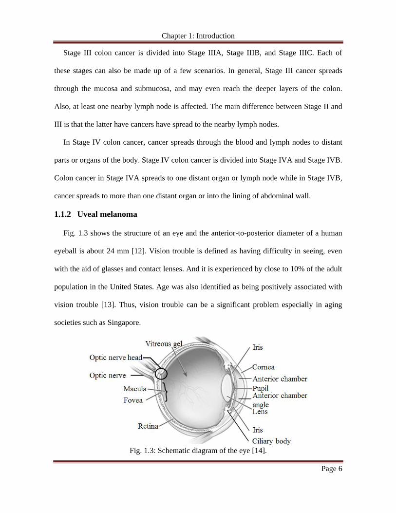


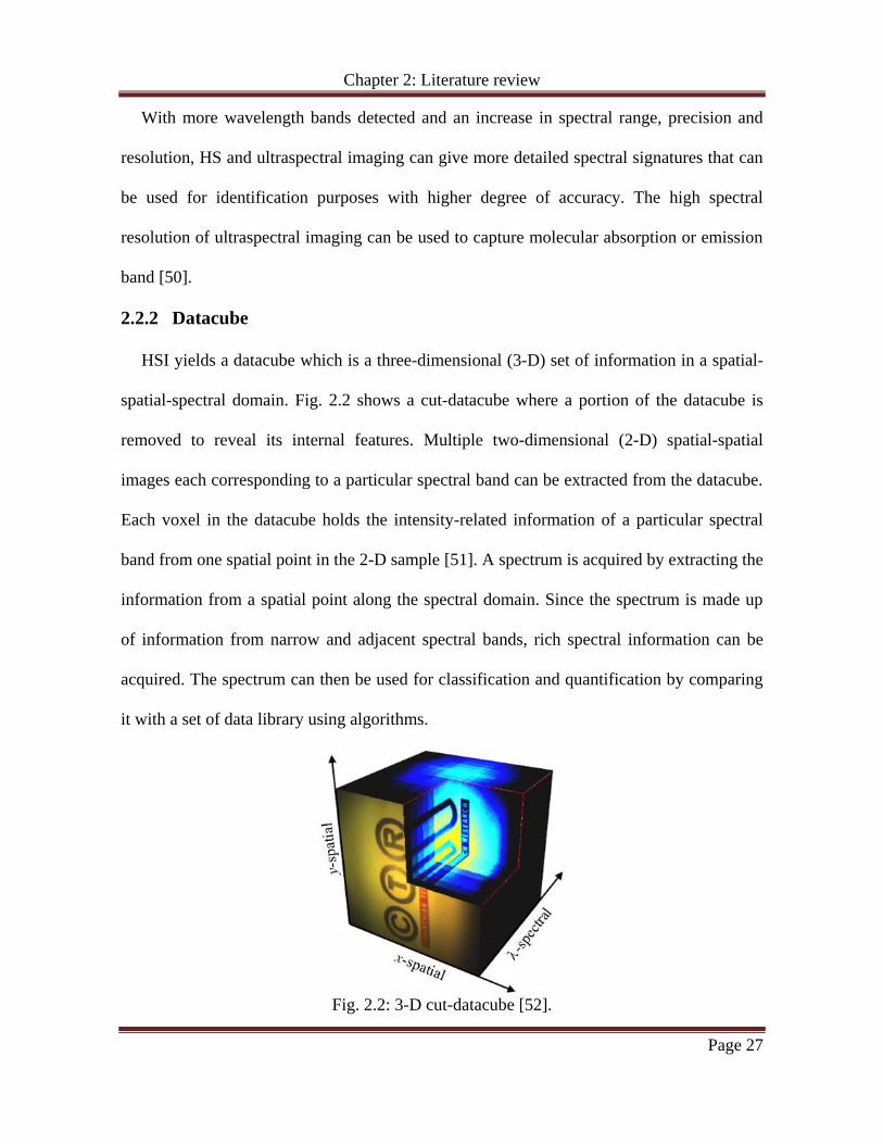


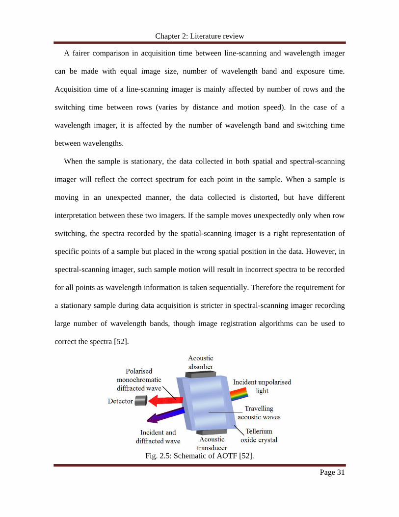


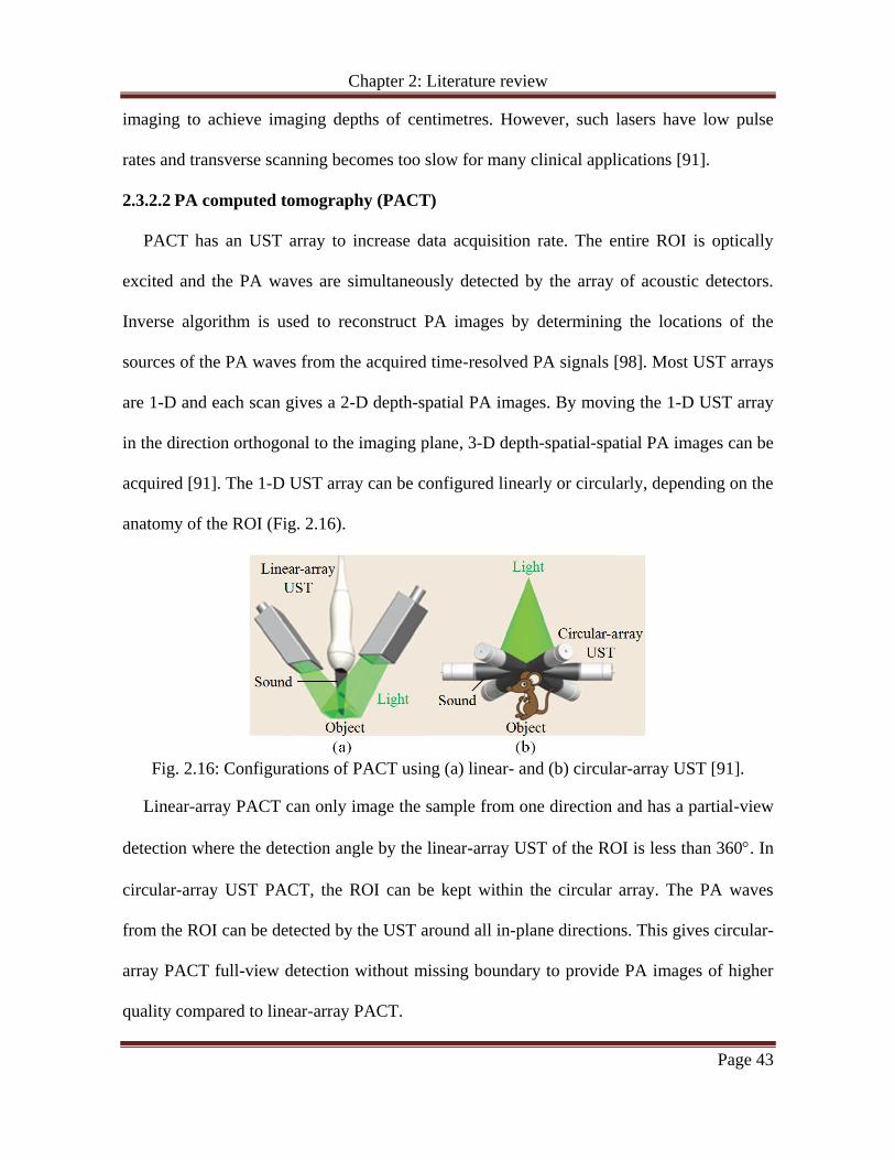


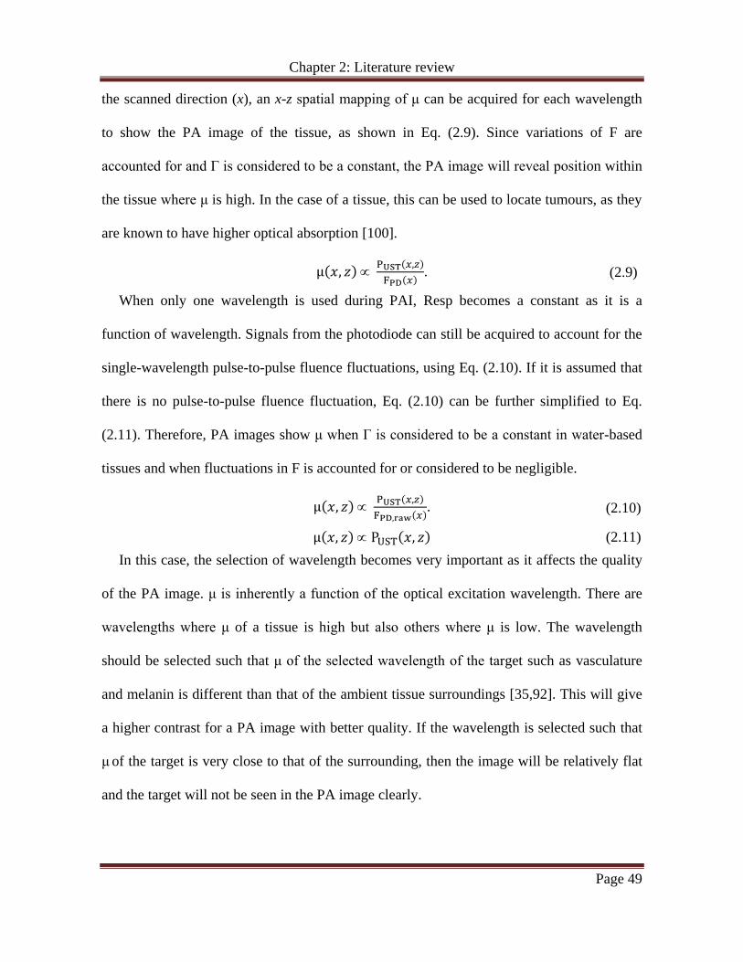


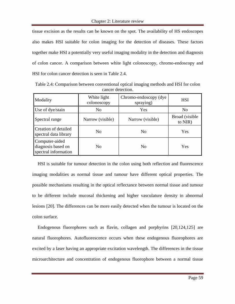


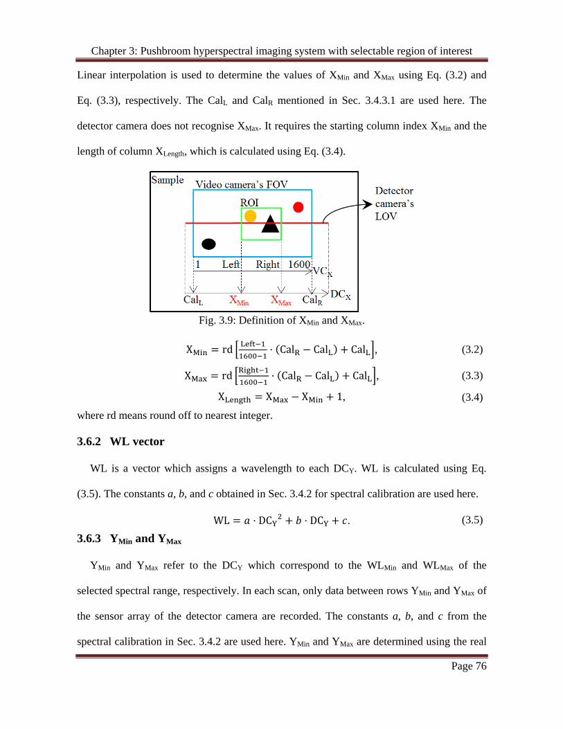


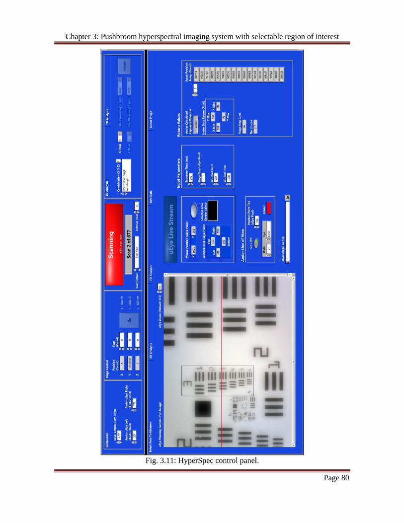


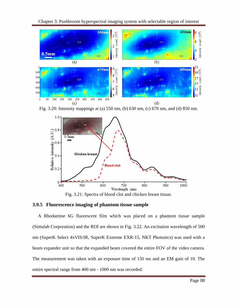


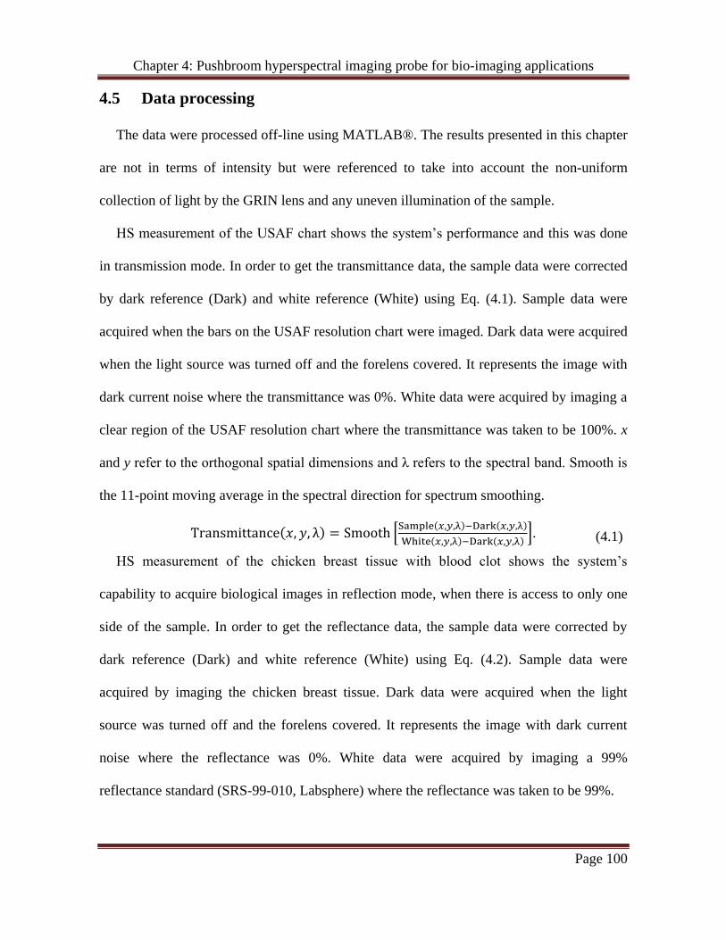
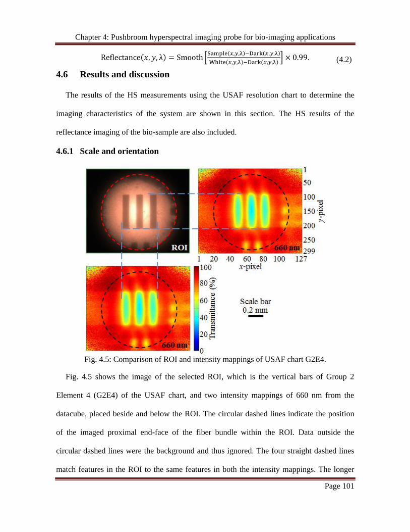


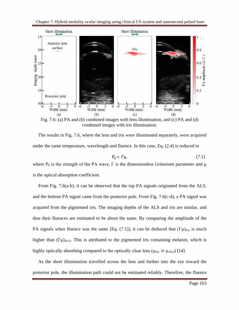


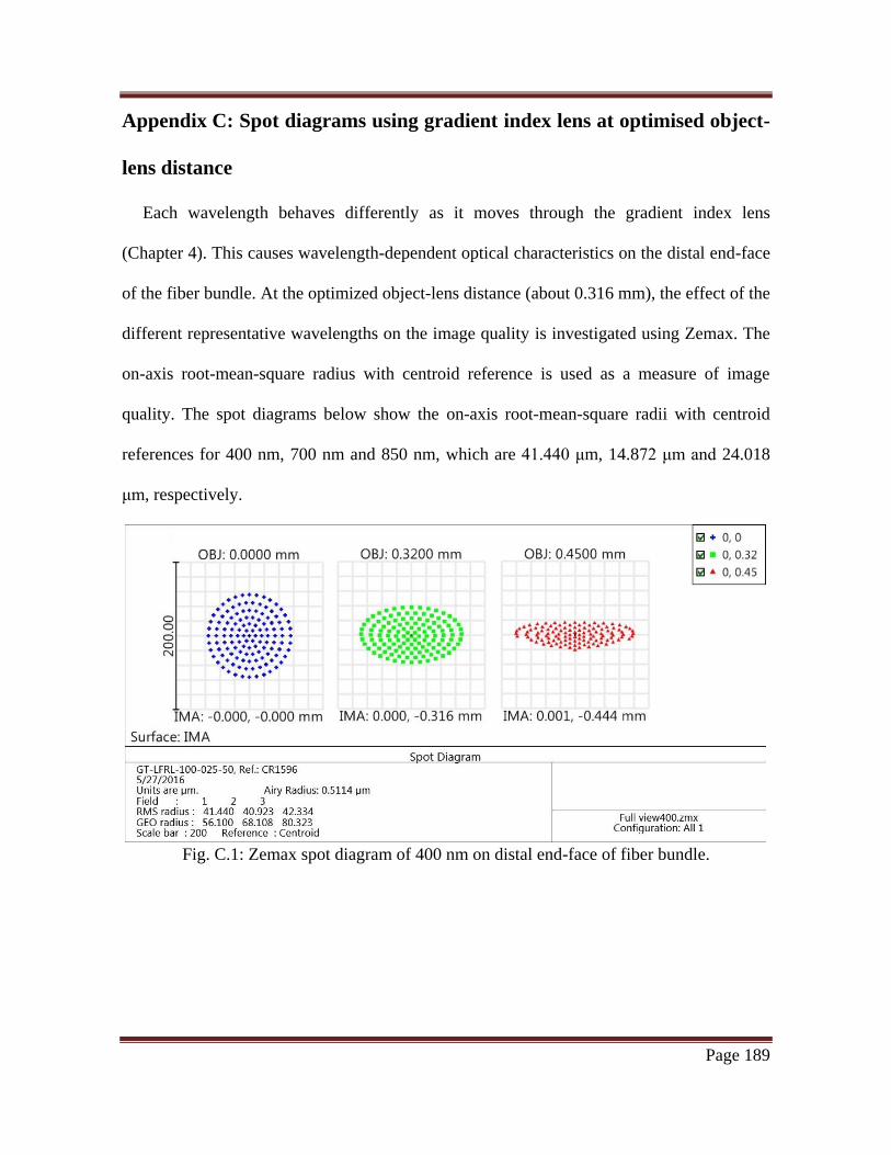


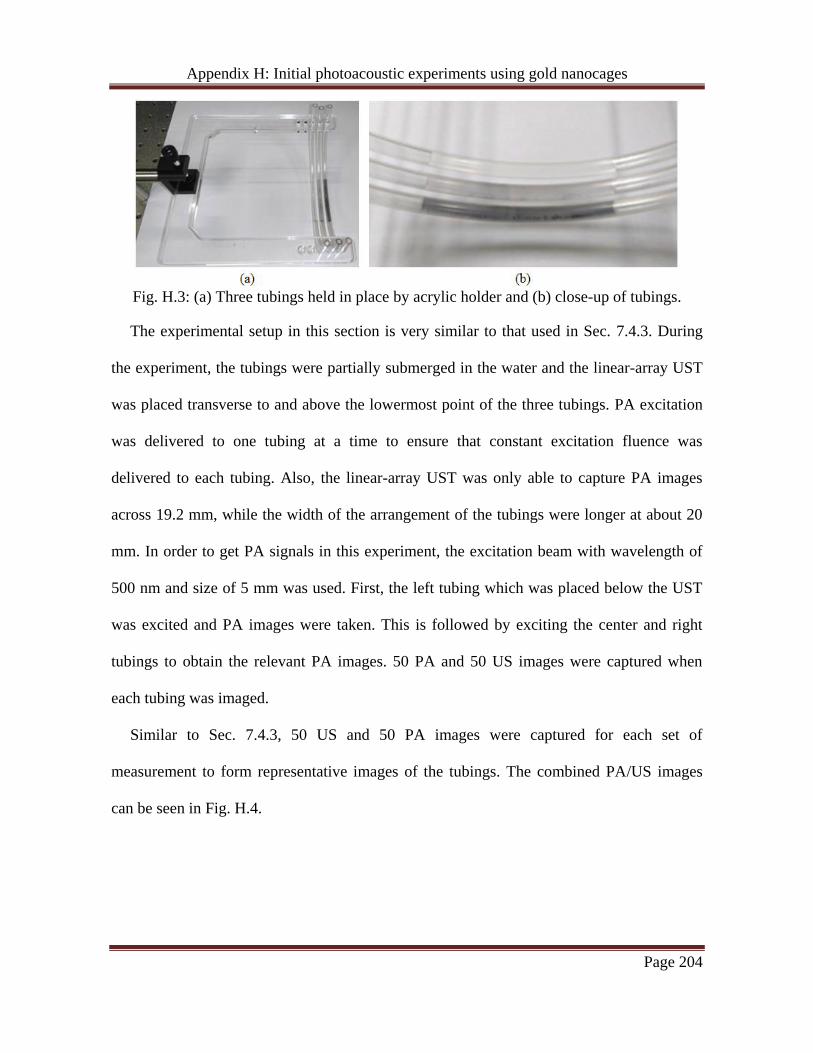
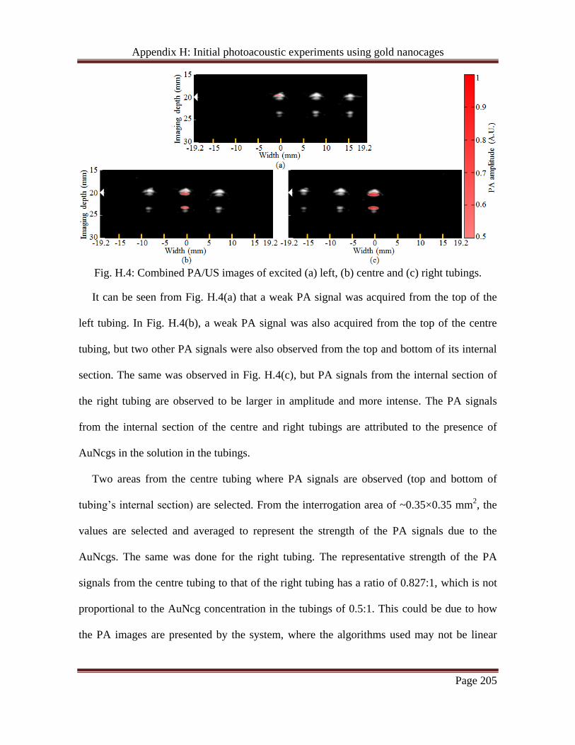


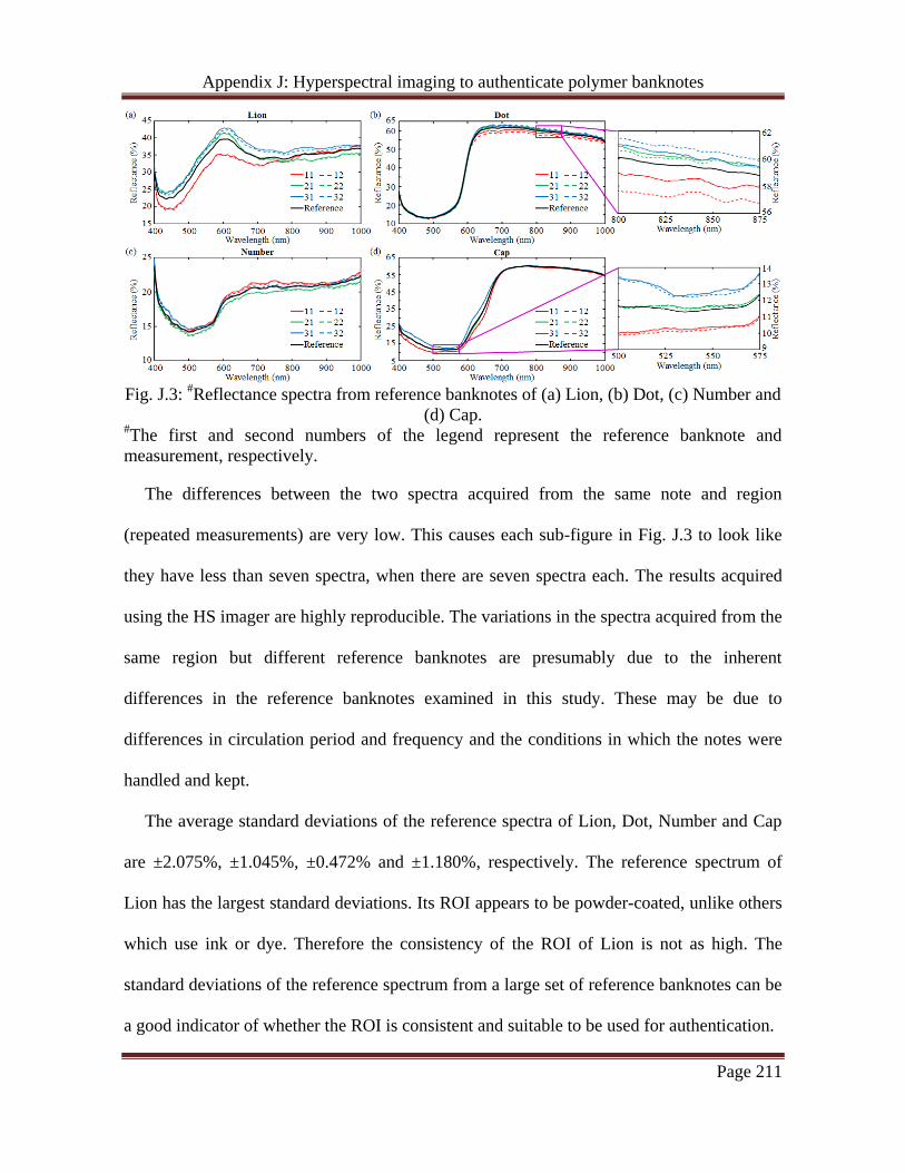


![MANETs: QoS and Investigations on Optimized Link …...namely, proactive or table-driven, reactive or on-demand and hybrid routing protocols [5]. Hybrid routing protocols are designed](https://static.documents.pub/doc/80x56/5f521eeffd78f944863d0ef1/manets-qos-and-investigations-on-optimized-link-namely-proactive-or-table-driven.jpg)


