Ion Acoustic Solitons in a Plasma: A Review of their Experimental Properties and Related

Theories

This article has been downloaded from IOPscience. Please scroll down to see the full text article.

1979 Phys. Scr. 20 317

(http://iopscience.iop.org/1402-4896/20/3-4/004)

Download details:

IP Address: 195.134.79.208

The article was downloaded on 14/05/2013 at 16:09

Please note that terms and conditions apply.

View the table of contents for this issue, or go to the journal homepage for more

Home Search Collections Journals About Contact us My IOPscience

Physica Scripta. Vol. 20,317-327, 1979

Ion acoustic solitons in a plasma: A review of their experimental properties and related theories M. Q. Tran

Plasma Physics Laboratory, Department of Physics, University of California at Los Angles, Los Angeles, Calif. 90024, U.S.A.

Received October 12, 1978; revised version February 20, 1979

Abstract where D is the dispersion relation. Due to dispersion, the beat mode (U, + w Z , k l + k z ) may not satisfy the dispersion Iori acoustic solitorls in a plasma: a review o f their experimental properties

and related theories. M. Q. Tran (Plasma Physics Laboratory, Department of Physics, University of California a t Los Angles, Calif. 90024, U.S.A.). Physica Scripta (Sweden) 20, 311-321, 1919. D(W1 + Wz , k l + k2) # 0 ( 2 )

A review of experiments and theories on ion acoustic solitonsispresented. Taking into account quadratic nonlinearity in the fluid equations leads to the Korteweg-de Vries (KdV) equation which predicts the existence of solitons. Experimental confirmation of their existence came with the availability of plasmas with large Te/C which allows us to minimize damping. However, the experimental datas on the dependency of Mach number vs. soliton amplitude clearly shows a discrepancy with the prediction of the KdV equation. The recent theories do include the effects of finite ion temperature and those due to the trapped electron population. The inclusion of nonlinearity of order higher than quadratic leads to the notion of dressed solitons the dynamic of which has been studied numerically. A discussion of other nonlinear equations describing ion acoustic waves will also be presented.

and therefore is not a normal mode of the system. The non- linear coupling t o a higher order mode is thereby stopped. Nonlinearity and dispersion are the necessary ingredients to obtain soliton solution for a nonlinear wave. However. although nearly all types of waves in plasma present dispersion. and the plasma itself behaves like a nonlinear medium, only a restricted number of waves is known to admit soliton solution. Konlinear ion acoustic waves do exhibit soliton solutions and have been well investigated both theoretically and experimentally. The present report tries to summarize the studies which have been performed in this domain.

1. Introduction 2. The Korteweg--de Vries (KdV) equation

The linear properties of waves in a plasma were for a long period sufficient t o explain adequately the observed phenomena. How- ever, it was soon perceived that a nonlinear treatment of the basic equations could provide a much richer harvest of results. Parallel progress in numerical simulations and experimental techniques allows us to confirm the theory and gives a strong stimulation to the study of nonlinear properties of waves in a plasma.

In this report we would like t o discuss the properties of ion acoustic solitons. A soliton is a nonlinear perturbation that exhibits a remarkable and characteristic property: after a collision, the emerging solitons have the same shape they had before the collision. By analogy with other quantum quantities which are also conserved, the name soliton was coined to define any nonlinear perturbation that exhibits this property. For simplicity, we shall also admit that the soliton has a non-vanish- ing amplitude only over a limited range [ 1 ] .

A soliton results from the balance of two effects: nonlinearity and dispension. Nonlinearity by coupling together different modes (a1, k l ) ( w z , k , ) gives rise to higher order modes (0, t w 2 , k , + k z ) , This process leads t o the well known wave steepening phenomena: the leading edge of the wave steepens as the perturbation moves (Fig. 1). Would it not be stopped by some other physical phenomena, the wave steepen- ing leads to wave breaking: at one position x, the wave ampli- tude becomes multi-value, a situation which is nonphysical. Dispersion is one of the phenomena which prevents the wave breaking, as is explained below. Let us consider two normal modes of the plasma, (a1, k l ) and ( W Z , kz) .

The fluid model of the plasma can be used to describe the ion acoustic soliton [2. 31. The one dimensional basic equations are:

~ the ion continuity and momentum equations:

an, aniui -+- = 0 a t ax

au, all, - + + U , - = E a t ax

( 3 )

(4)

~ ~ the momentum equation for the electrons. As the electron mass me is negligible, the right hand side of the equation is negligible:

0 = neE-- ane ax

- the Poisson equation:

- ni-rzn, aE _ - ax

In eqs. (3)-(6). ni. U,. ne refer respectively t o the ion density and velocity, and the electron density. E is the electric field. Distances are normalized t o the Debye length Ade , densities t o the unperturbed density and velocity to the ion acoustic speed (re/Mi)':2.

D(01,z ,k1 ,2: l = 0 (1) Fig. 1. Wave steepening process. [ 5 ]

Physica Scripta 20

3 18 M. Q. Tran

In the linear approximation, eqs. (2)-(6) give the well known dispersion relation

w = kjl-;) (7)

which shows that for large k, ion acoustic waves are dispersive. For perturbations of small but finite amplitude, Washimi and Taniuti [2] introduce the following development:

ne,i = 1 + En$ + c2nk:)i + . . . = € u p + E%{,') + . . . ui

. . . E = E 3 / 2 $ 1 ) + E5/2@'(2) +

and the stretched coordinates:

( = ?(x - t ) q = E3'2X

where E is an ordering parameter. In the first order in E , the set of fluid equations give:

which can be integrated to yield: n(l) = (1) = (1)

e ni ui In second order in c we get

Eliminating second order terms and n!') and U!') we obtain an equation for nonlinear ion acoustic perturbation

It is to be noted that eq. (19) can also be derived from the fluid equations (3) through (6) using the stretched coordinates

( = (x - t ) P

and

7 = E 3 9 (20) The detailed derivation using these last stretched coordinates will be given in Section 7 of this review.

Equation (19) is the well known Korteweg-de Vries (KdV) equation [4] , and describes the nonlinear behaviour of ion acoustic waves. The convective term nil) ank"/at describes the nonlinearity, and the third derivative term a3 nL1)/at3 reflects the dispersion. An inspection of eq. (13) shows that the KdV equation is not invariant under the change nil) + -nil). More precisely, an initial depression of density will evolve into a wave train whereas a density compression (n!$ > 0) will break up into solitons [3, 5-81. The ion acoustic soliton is a com- pressional pulse whose spatio-temporal dependence is given by:

Physica Scripta 20

Applled potential 1V/dlv

Time, 5psec/d1v

Fig, 2. Time evolution of a nonlinear compressional perturbation measured at different positions according to [ 9 ] . The perturbation first steepens, then breaks into solitons.

where M is the Mach number equal to the ratio of the soliton velocity to the ion acoustic speed. The amplitude the width D and the Mach number M are related through:

M-1 = 6 4 3 (22)

D = ( 6 / 6 r ~ ) " ~ (23)

The first experimental observation of ion acoustic soliton has been made by Ikezi et al. [9] in a Double Plasma (DP) device [ l o ] . The principal features of the DP device are the high electron to ion temperature ratio Te/T (TJT lCrl.5) and its capability of exciting large amplitude ion waves without generating pseudo-waves [ 1 11. A high temperature ratio Te/T ensures that an initial perturbation can propagate and break into solitons that are only slightly damped. The absence of pseudo- waves simplifies the interpretation of the experimental data. In the Ikezi et al. experiment [9], a large positive potential pulse is applied to the source plasma giving rise to a compressional pulse at the boundary x = 0 of the target plasma. As this perturbation propagates, its leading edge steepens as a result of nonlinearity. On the trailing edge a structure starts to form and finally breaks into a succession of compressional pulses (Fig. 2). Their velocity is higher than the ion acoustic speed C, and, consequently, the Mach number M is greater than 1. The Mach number increases while the width D of each individual pulse decreases with its amplitude 6n. A qualitative agreement between the experimental values and those derived from eq. (22) and (23) was found. In particular, the measured values of M in function 6n are larger than those inferred from eq. (22) (Fig. 3). More elaborate theories, which will be discussed provide a better quantitative agreement between theory and experiment.

The dependence of M and D on 6n suggest that each individual

0 0 2 0 , an -T

Fig. 3. Dependency of the Mach number M vs. the soliton amplitude according to [9]. M is defined as the ratio of the soliton velocity to the velocity of a linear ion acoustic perturbation. The straight line is the theoretical dependency obtained from the Korteweg-deVries equation.

Ion acoustic solitons in a plasma: A review of their experimental properties and related theories 3 19

~ : . ., ~ . , .

Fig. 4. Evolution of the shape of two colliding solitons before and aftei the collision [ 9 ] . The shapes of the two solitons emerging after the col. lision is identical to those they respectively have before the collision.

pulse is a soliton. By converting the DP into a Triple Plasma, Ikezi et al. [9] provide direct experimental confirmation of their nature. Solitons were generated at the two ends of the target plasma and interact at the center. After the collision the two emerging pulses retain their original shape (Fig. 4). This experimental evidence undoubtedly confirms that the observed nonlinear structures are solitons. It is also worth noting that, in agreement with the prediction of the KdV equation (19), only compressional pulse breaks into solitons. A large negative voltage pulse applied t o the source plasma will produce a wave train in the target plasma. i.e.. a perturbation, the amplitude of which swings from positive t o negative.

The number of solitons which evolve from a given initial perturbation has been studied by numerous authors [ 1 1- 141 . According to the inverse scattering method [6] which is used to solve analytically the KdV equation (19), the number of solitons is given by the number of bound states of the associated Schroedinger equation:

a* $ - + [E - V ( ( , Q = O ) ] I) = 0 3 t 2 The potential V ( [ , Q = 0) is related to the perturbation at x = 0 by

v($, t7 = 0 ) = --dnL’)(g, Q = 0 ) (25)

In Hershkowitz et al. [ l 11 experiment, a square voltage pulse was applied to the source plasma: the determination of the number of bound state of eq. (24) is just a classical problem of quantum mechanics. However, a square pulse is seldom used experimentally: coupling problems distort the applied signal. Usually a sinusoidal voltage pulse is applied t o the source plasma. An analytical solution t o this problem has been dis- cussed by Ikezi [12] . A qualitative agreement was found: the higher the amplitude of the initial perturbation, the larger the number of solitons. However, the number of observed solitons is higher than the one predicted theoretically. A better agreement between theory and experiment can be found if ion temperature effects are included in the KdV equation [13] .

Although many of the previously mentioned experiments [9, 1 1, 12, 141 involve the use of DP device, nonlinear ion acoustic perturbation can be launched by other methods. Cohn and MacKenzie [15] used photoionization t o produce a large localized density perturbation in a background plasma. Watanabe [13] launches large amplitude perturbation using the con- ventional grid excitation. In both cases, an initial compressional pulse was observed t o break into solitons.

Fig. 5. Recurrence of the initial waveform [12] . The initial wave-form reappears as the wave propagates.

Waveforms other than a sinusoidal pulse can also be used t o produce solitons. Ikezi [12] has shown that a sinusoidal nonlinear acoustic wave also gives solitons. Furthermore, the recurrence phenomena were also observed. The wave first breaks into solitons. However, at further distances the original wave form was restored (Fig. 5 ) . A train of solitons can also be obtained in the target plasma of a DP device when a ramp excitation [16] is applied to the source plasma. For small applied voltage, the resulting structure looks like a collisionless shock [17] , with a “shock front” and an oscillatory train. However, it has been verified numerically by Tran et al. [18] that under experiment conditions of [ 161 , the so called “laminar shock” is in fact a train of solitons. A similar con- clusion was reached by Gurevich and Pitaevski 1191, who have studied analytically the solution of the KdV equation with a step function as an initial perturbation.

In conclusion, many experimental results did confirm the prediction of the simple KdV equation. However, quantitiative discrepancies exist between theory and experiment. The differ- ent theoretical models which will be reviewed in the next chapters give a closer agreement.

3. Finite ion temperature effects on solitons

In a real plasma, the effect of finite ion temperature cannot be neglected: in a DP device, the electron t o ion temperature is of the order of 10-20. These effects can be described by either a fluid or a kinetic theory. In the fluid model, the momentum equation (4) is modified t o

where an adiabatic equation of static for the ion was assumed. By the same method as the one used t o derive the KdV equation (19), a KdV equation with modified coefficient is readily obtained [20, 21 J .

where [‘ is defined by (x - d l - 3TJTe t ) .

amplitudes is now given by: The relation between the Mach number M and the soliton

1 6 n ( l + 6Ti/Te) M = 1 + - 3 (1 + 3Ti/Te)3’2

For a typical value of Te/Ti 10- 15, eq. (28) gives only a slight increase of M and does not account for the observed discrepancy between theory and experiment.

Sakananka [22] has proposed another approach to treat

Physica Scripta 20

320 M. Q. Tran

the nonlinear equations (3), (19), ( 5 ) , and (6). The method was originally used by Moiseev and Sagdeev 1171 in their treatment of soliton and collisionless shock waves. Instead of looking for a nonlinear equation for space and time evolution of the pertur- bation, it is much simpler to search only for a stationary soliton of the fluid equations in a frame moving at a certain velocity M. No development in power series [cf. eqs. (8&(10)] is per- formed. The solutions, when they exist, are therefore valid up to amplitudes much larger than those described by the KdV equation. However, no information about the space-time evolution of an initial perturbation can be obtained.

In a frame moving with velocity M , the ion density ni is given by

1”’ 1 ‘ I 2 (29)

In eq. (29), @ is the potential associated with the perturbation and is normalized to (Te/e). The Poisson equation (6) combined with eqs. ( 5 ) and (29) yields

- - - exp {a) - ni(@) aza ax2

A first integration of (30) gives

J(aip/ax)2 = -U(@) (31)

where U(@) is defined by

Equation (32) has a mechanical interpretation. It describes the motion of a particle in the potential U(@): in this analogy, @ represents the particle position and x the time. Integrating eq. (31) then gives @ as a function of x. The dependence of M vs. the soliton amplitude is given by

The use of relation (33) gives a better fit between theory and experiment as shown in Fig. 6 [ 131.

Many effects of finite ion temperature cannot be described by a fluid model. Kinetic effects have been discussed by various authors [23-261. Ion Landau damping [25] as well as electron Landau damping [23] contribute to damp out the soliton. Due to the distribution in energy of the ion, ions with a kinetic energy less than the potential energy of the perturbation will be reflected. Experimentally, a precursor or reflected ion is observed in many experiments [9, 12-15]. A detailed discussion of the importance of ion Landau damping and ion reflection can be foundin [25] and [26].

4. Trapped electron effect

The electron behaviour is also strongly modified by the non- linear potential of the soliton. It is usually assumed that elec- trons are isothermal during the passage of solitons [cf. eq. ( 5 ) ] . This assumption is only valid if they can be thermalized by collisions with the wall of the device [9]. If this constraint is released, electron trapping in the soliton potential may well occur, provided the bounce period vbl is smaller than the

Physica Scripta 20

. ”” 0 0.1

Amplitude n/no

Fig. 6. Comparison between the experimental dependency of the Mach number on the soliton amplitude 6n and the prediction of different models which takes into account finite ion temperature effects [ 131. The dots (.) are the experimental points, the solid line (-) is the prediction of the KdV equation, the line (--) is the values obtained from eq. (21) and the line (--) is the values from eq. (26) .

transverse transit time v i ’ between the center of the machine to its wall:

(34)

L is the radius of the machine, h the width of the soliton, and @ the potential associated with the soliton. The condition (34) is met in most experiments [27]. Experimentally a flat topped electron distribution function, characteristic of the presence of trapped electrons [28-301 has been observed in an ion acoustic soliton [27]. Figure 7 shows the electron distribution in a soliton and outside a soliton. It is clearly apparent that inside a soliton, the distribution function presents a plateau at low energy.

The electrons can now be separated into two categories: the free electrons and the trapped electrons. To describe the electron density, Schamel [31,32] used the following expression

Fig. 7. Measured electron distribution function inside a soliton (curve 1) and outside a soliton (curve 2) according [ 2 7 ] . Note the flattening of the distribution function a t low energy when it is measured in a soliton. This phenomena is characteristic of the presence of trapped particles. Curve 3 is the electron distribution function in the absence of any perturbation.

Ion acoustic solitons in a plasma: A review of their experimental properties and related theories 321

In eq. (35), Tef and Tet are respectively the temperature of free and trapped electrons. is a parameter equal to 1 for solitary waves. Using Washimi and Taniuti’s method [ 2 ] , Schamel [32] derives a modified KdV equation for the potential perturbation;

asp. 1 a3@ a t ax 2 ax3

-+- - = o (36)

Equation (36) admits soliton solution [32]

@(x) = 6 @ s e ~ h ~ [ x / [ 1 5 n ” ~ / ( 6 @ ” ~ ( 1 - Tef/Tet))] liZ] (37) The relation between the soliton amplitude and the Mach number is now given by

The relation (38) has been plotted by Ichikawa and Watanabe [33] for different ratio refire, (Fig. 8). It appears that an adequate choice of Tef/Tet can provide a good fit between theoretical and experimental results.

5. Effect of higher order nonlinearity

In the preceding sections, attempts to interpret experimental data by including effects such as finite ion temperature Ti or electron trapping in the soliton potential were presented. More recently an attempt t o interpret the data by including both high order nonlinearity and finite ion temperature has been proposed [341.

The basic equations are: - Vlasov equation for the ion.

- Boltzmann’s equations

(39)

- and Poisson’s equation

a 2 @ ax - = n e - / f d v

f(x, v, t) is the ion distribution. The procedure is t o look for a stationary solution of eq. (39) t o (41) in a frame moving with velocity M . Defining:

x = (x - M t )

densify perturbation 6n no

Fig. 8. Comparison between the measured values of the Mach number M for different soliton amplitude and theoretical predictions from Schamel’s theory [ 321 as reported in [ 331. The broken line with dot ( -.-) is from KdV equation. The dotted lines are curves calculated from Schamel’s theory with arbitrary parameter p = T,f/Tet. The bars are experimental results from [ 9 ] . The solid curves (-) are derived from a more recent theory that took into account three waves coupling and ion temperature effect [47] .

eqs. (39) and (41) reduces to

(42) af av

- (M - v) f ’(v, x) - sp.’(x) - = 0

@”(X) = ne - f dv (43)

where the prime denotes differentiation with respect t o X. Separating the distribution function f(v, X) into two parts

f (v , x) = fo(v> + f I ( ? x) (44) where fo(v) is time and space independent and f l (v ,X) the dependent part, equation (42) becomes

-(M-v)f;(v,x)-@’(x) -+- = 0 [2 3 (45)

The solution of (45) is obtained by iteration. In the lowest order (45) gives

which can be integrated with respect to X t o yield

(47)

Equation (47) is then substituted for afl/av term in eq. (45) t o give fi (v, x) in the second order.

The procedure can be repeated to any order. Expanding now (40) in power series of Q, and substituting in (43) gives

= aG2 + b@’ + ca4 + da5 (49)

where:

dz d t

a = - ( T e / 2 z ) - + 1

b = (1/6)(Te/2T)2 d3Z/dC3 - 1/3

c = (1/96)(Te/2z)3 d5Z/dC5 - 1/12

d = (1/2880)(Te/2Ti)4 d7Z/dC7 - 1/60 (53)

5 is the ratio of the perturbation velocity t o the ion thermal velocity and Z(C) the Fried and Conte function.

Putting b = c = d = 0 just gives the kinetic dispersion relation of ion waves. For the rest of the discussion it was assumed that T e / z is high so that the imaginary part of Z could be neglected compared t o the real part. This assumption is consistent with the experimental observation that ion acoustic soliton exist only if damping or resonant wave particle interactions are not too strong.

Equation (49) just gives the soliton solution if c = d = 0. The relation between amplitude and Mach number also agrees with the stationary solution of the KdV equation when = 0 [27 ,28] . Including in eq. (49) only the cubic nonlinear term (i.e., c # 0, d = 0) we obtain as the following stationary solution

Piiysica Scripta 20

322 M, Q. Tran

1 I O

5 105

s

I O 0 0 0 1 0 2

20

D

T 10

I

0 01 0 1 0 3

AHPLl lUOE "/"p

Fig. 9. The velocity ( U ) and width of an ion acoustic soliton in depen- dence of density perturbation n/no [34]. Bars (-) are experimental data from [12 ] and open circle ( 0 ) from [13]. The solid lines are computed from eq. (54) which takes into account cubic nonlinearity as well as finite ion temperature. Dotted lines is obtained from KdV equation ion.

For the case abcd # 0, no analytic solution has been found and eq. (49) has to be solved numerically. However for experi- mentally observed soliton (CP<30%) an expansion up to the cubic term is accurate enough [34].

Watanabe [34] has plotted the Mach number dependency vs. soliton amplitude for different cases: Te/Ti = m, KdV equation with finite ion temperature and results from eq. (54) (Fig. 9). As we have already noticed, neither the KdV equation with # 0 cannot account for the measured values. The velocity predicted from eq. (54) is however in good agree- ment with the experimental datas.

= 0 nor

6 . Ion acoustic solitons in a multi-ion plasma

The introduction of a second ion species in a plasma modifies the ion acoustic wave properties in the linear as well as in the nonlinear regime. In the linear regime, there now exist two ion acoustic modes [35], called the light and heavy ion modes; they are the modification of the modes which exist in the plasma of one component, respectively of light ion and heavy ions. Experi- mental studies of linear ion waves [36-371 confirm the existence of the two ion wave modes. The measured dispersion relation showed a good agreement between theory and experiment.

In the nonlinear regime, White et al. [38] have discussed the stationary solutions of the fluid equation which describes a two component plasma, for example an Ar-He plasma. Two different types of structure were found, depending on the amplitude of the nonlinear perturbation. In a one component plasma, the fluid equations admit soliton solution only if the kinetic energy of the ions is sufficient to allow them to over- come the potential hill @ of the soliton. In a two component plasma, soliton solutions are found, provided @ is small enough so that both the light and heavy ions can overcome the potential hill. In contrast to the one component case, stationary solitons still exist in the case where CP is high enough to reflect the light ions but not the heavy ions. The latter type of solution is not a soliton but a collisionless shock wave since the upstream region has different characteristics than the downstream one. In the upstream region, the shock pushes ahead all the light ions, which are consequently absent in the downstream region. Figure 10 shows the domain of concentration a of light ions Physica Scripta 20

M

1.55

1.48

- 1.40

- -

,134

- 1 2 6

Fig. 10. Domain of existence of soliton and collisionless shock in a two component plasma [ 381.

where solitons or shock can be found. It also gives the range of Mach number over which these solutions exist. [In [38] the Mach number is defined as the soliton or shock velocity divided

As in a one component plasma, nonlinear acoustic pertur- bation can be described by a KdV equation [39]. The fluid equations for two component plasmas are:

by (kB TeIMheavy ' I z I

anj anjuj - at ax -+- - 0 j = 1 , 2

- -neE _ - ane ax

aE - = 1 nj-ne ax j = 1

( 5 5 )

( 5 7)

In the preceeding equation, j denotes the ion species, 1-1 the mass ratio M 2 / M 1 > 1 and a the light ion concentration (a = no l Inoe). Time t is normalized to w i t = [noe2(1 - a + ap)/eoM2] - ' I2

and velocity to the actual sound velocity in a two component plasma C, = [kBTe(l - a + ap)/M2] ' I 2 . This normalization allows us to use the stretched coordinates defined by eqs. (1 1) and (12).

Using the same method as the one used in Chapter 2, we find the following relation for the first order terms:

nil) l - a + a / J = - a + ,(l) =

1 Pa 1 - a

Ion acoustic solitons in a plasma: A review of their experimental properties and related theories 323

L- e , -

Eliminating second order terms in eq. (60) to (65) with (59) we get the KdV equation for a two component plasma with = 0

Soliton solution of eq. (66) presents an amplitude 6n given by

3(1 - - C Y + (~l.1')

(1 - a + cup) 6n = 6(M- 1)

In eq. (67), M is defined as the soliton velocity divided by the ion acoustic velocity (C,) in the two component plasmas:

-a+cup)- kbTel M2 1'2

Plot of Sn/(M - 1) vs. (Y is reported in Fig. 11. Compared to the case of one component plasma (a= 0% or cu = 100%) it is evident from Fig. 11 that the introduction of the second ion species reduces the soliton amplitude a for a given M .

Extensions of Tran and Hirt's work [39] have been performed by Tran [40] to include ion temperature effect, by Tagare [41] who took into account the effects of multi-species of positive as well as negative ions.

An experimental investigation of the properties of ion acoustic soliton in an Ar-He plasma has been performed by Tran and Hollenstein [42]. It was shown that in an Ar plasma the introduction of a few percent of light ion is sufficient to prevent the soliton formation (Fig. 12). Ion Landau damping and ion reflection by the potential hill have both increased since the added He ions are resonant with the perturbation: these two processes are responsible for the non-formation of the soliton. The introduction of Ar ions in an He plasma affects the soliton formation much less. Experimentally solitons were ob- served in He plasma containing up to 30% of Ar. The detailed study of the relation between M and Sn leads to the conclusion that fluid models such as the KdV equation cannot fit the experimental data. A kinetic treatment which correctly describes the reflected ions has been used by Tran and Hollenstein [42] to interpret their data.

7. Dressed soliton

The KdV equation (1 9) accounts for nonlinear quadratic effects. It is legitimate to wonder about effects of higher order terms

+ 'C', 2 2 . . IC'. &:.. 5C'. m... -0.:. 8C.I. 9 0 % '00''.

Fig. 11. Variation of the ratio of the soliton amplitude 6 n to (M - 1) in dependency of the concentration of light ion [39]. The Mach number M is defined as the ratio of the soliton velocity t o the ion acoustic velocity in a two component plasma. f i is the ion mass ratio.

't ,\ a=l%

Fig. 12. Evolution of a soliton in Ar/He plasma [43]. cy is the He ion concentration.

in the expansion [eq. (8) and (lo)]. In Section 5 we have shown that stationary solutions of kinetic equations for ion waves in the limit T, S did exhibit different properties whether or not terms of order higher than quadratic were included. The limitation of the method presented in Section 5 is obvious: it does not allow us to study the evolution of an initial perturbation nor the interaction of many solitons. Indeed, recent theories [43-451 did allow us to predict the evolution of an initial perturbation when higher order terms of the expansion (8)-(10) are used. In the following we shall present the discussion of Ichikawa et al. 1431 on the effect of the cubic term.

The basic equations are the usual fluid equations, that we shall recall for clarity:

an a at ax - + -(niui) = 0

a aui a@ at ax ax -U. + U . - = --

We shall also introduce the stretched coordinates = E'"

(x - t) and r = ~ ~ ' ~ t and we also expand ni, ui, ne and @ in series of power

(73)

(74)

= ,@(I) + + E3 @[3) + . . . (75)

The first order term in e of eqs. (69)-(72) just gives the relation [eq. ( 1 4 ~ @(I) = (1) = (1) = np

U1 n1

In second order E, we get

Together with relation (14), eqs. (76 t (78) yield the wellknown KdV equation

Physica Scripta 20

324 M. Q. Tran

In third order in E , we obtain

In this approximation, the perturbed potential @ results from two contributions @ = @(1) + @(2)

where solution of the KdV equation (79), describes the fundamental nonlinear effect and a('), solution of eq. (83), the interaction of the fundamental nonlinear wave and higher order dispersion. Steady solution of the coupled equation (79) and (83) has been computed by Ichikawa et al. [43]. In a frame moving with velocity M , stationary solutions are given by

@(x -Mt ) = 3(M- 1) sech' [ i"; - (x -MO]

1 9 4

+ -(M - 1)' sech'

1 x ( M - l)(x -Mt) tanh i - 8 + 7 sech' p- 1); -""I]

Figure 13 shows the shape the solution (84) for a M - 1 = 0.1. The broken line shows the core as derived from the KdV equation and the full line the solution obtained from eq. (84). We saw that the higher order clouds did lower the amplitude of the perturbation. This new perturbation is known as dressed soliton.

A numerical study of the set of equations (79) and (83) has been performed by Konno et al. [46]. The evolution of an initial perturbation given by:

0.3 I '9 o . 2 i J

0 1 ,

'. -2 -I 0 * I ' 2

02 Fig. 13. Plot 'of a dressed soliton given by eq. (84) with M - 1 = 0.1. The dotted line is the core, solution of the KdV equation. [43]

Physica Scripta 20

0

-x)60-3185-2530 -1255 0 12s 25303785

Fig. 14. Evolution of the shape of a dressed soliton. The initial potential is a KdV soliton. The thin line represents the KdV soliton. The second order clouds represented by broken lines develop around the KdV core. Simultaneously a wave train is emitted behind the soliton. [46]

@([, 7 = 0) = @by[, 7 = 0) (85)

where @ & I ) @ , r = 0) is a soliton solution of the KdV equation, is presented in Fig. 14. It is observed that around the KdV core, the clouds develop and that a sinusoidal wave train is emitted. Turning now to the head on collision of two solitons, one must notice that in contrast to the case of the KdV equation where, aside from some phase shift, the soliton velocities are conserved, there exist now an acceleration of the smaller soliton and a deceleration of the larger one (Fig. 15). In another case where the amplitude of the two colliding solitons are similar, it was observed that the clouds rearrange themselves to equalize the amplitude of the colliding pairs.

8. Other equations describing nonlinear ion waves 8.1. The Boussinesg type of equation [47] The dispersion relation for ion acoustic waves is given by

k2 0 2 = -

1 + k Z

It can be approximated by o = k[ l - k2/2] and the KdV equation (19) has been derived under this assumption. Another equation, the improved Boussinesg equation, could be derived for waves which have a linear spectrum given by [eq. (86)]. As

632.5 I )!(I

W I . #/ + 316.2

9 3 . 2 0 63 2 E

Fig. 15. Interaction of two dressed solitons represented by the thick line. The KdV solitons are drawn by the thin line and the second order cloud by the broken line. The trajectories of the two colliding solitons are also represented. (Thick line: trajectories of the dressed soliton, thin line: free motion of the soliton and broken line: KdV soliton trajectories). The small soliton is accelerated while the larger one is decelerated during the colision. [46]

Ion acoustic solitons in a plasma: A review of their experimental properties and related theories 325

Makhankow has shown in an elegant way [47], the dispersion relation (86) could be written as

w2(1 + k 2 ) = k 2 (87) or in the operation form

A nonlinear equation can then be written simply by adding t o eq. (87) a nonlinear term a/ax(@)" which is similar to the non- linear term in the KdV equation:

or equivalently

Equation (88) approaches the usual Boussinesg equation in the limit of long wave length k < 1 :

The linear part of eq. (89) leads t o the dispersion relation

w 2 = k*(1 - k 2 ) (91)

which also approximates the dispersion relation (86) in the limit k < 1. Numerical solutions of eq. (89) have been computed by Bogolubsky [48]. Contrary t o the KdV equation, the solution of which has a direction of propagation, solutions of eq. (88) are symmetric, i.e., solitons do move in opposite directions. Solitons shape and amplitude are not preserved after a collision.

8.2. The Benjamin-Bona-Mahony equation Broer and Sluijter [49] have presented a new method to obtain an equation for nonlinear ion waves. This method is based on the use of an approximate Hamiltonian. Basically, first one proves that the fluid equations (69)-(72) are equivalent t o a Hamiltonian system derived from an Hamiltonian H . Once the existence of a Hamiltonian H is proven, we can use a more trac- table approximate Hamiltonian Ha. In fact, the exact form o f H is not required: it is sufficient t o prove its existence only.

For waves of short wavelength, an approximate Hamiltonian Ha can be selected as

Ha = dx[;(l + V ) U ; + ~ ( V ) - ~ ( V ) ~ ]

where Vis defined by

The canonical equations now become:

a av 1 a3v at 2 a t a 2 ax

- .- -- ( U i + uiv)

a aui 1 a%, a t 2 atax2 ax

- - -- ( V - i P + $24 ; )

(93)

(94)

Equations (93) and (94) can be reduced to a Benjamin-Bona- Mahoney type of equation [SO]

aui 1 asui a = -- [u i+Qu;] a t 2 a t a x 2 ax This equation is much less known than the KdV equation (19). However as noticed by Broer and Sluijter [49] it describes much better the behaviour of wave with large k. Therefore the approxi- mate Hamiltonian Ha has a larger domain of validity than the one which would lead t o the KdV equation.

8.3. Effect o f dissipation The KdV equation (19) and the various other equations we

have just discussed did not include any dissipation. As it has been shown [51], dissipation did lead to new phenomena in soliton formation: not only does the soliton amplitude decrease while it propagates, but also a tail is formed behind it.

The two equations which were solved numerically in [51] were KdV-Burgers equation:

and a KdV equation for an ion acoustic soliton in presence of weak ion neutral collision (28)

aui aui 1 aui - + t i - + - - + + * u i = 0 ar a t 2 at3 (97)

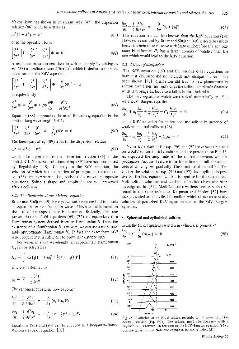
Numerical solutions for eqs. (96) and (97) have been obtained for a KdV soliton initial condition and are presented on Fig. 16. As expected the amplitude of the soliton decreases while it propagates. Another feature is the formation of a tail, the ampli- tude of which grows gradually. The structure of the tail is differ- ent for the solution of eqs. (96) and (97): its amplitude is posi- tive for the first equation while it is negative for the second one. Multi-soliton solutions and collision of solitons have also been investigated in [51]. Modified conservations laws can also be found in the same reference. Karpman and Maslov [52] have also presented an analytical formalism which allows us to study solution of perturbed KdV equation such as the KdV-Burgers equation.

8. Spherical and cylindrical solitons

Using the fluid equations written in cylindrical geometry:

0 ICC

NSTAHCE

Fig. 16. Evolution of an initial soliton perturbation in presence of ion neutral collision [Eq. ( 9 7 ) ] . The soliton amplitude decreases while a negative tail is formed. In the case of the KdV-Burgers equation (96) a positive tail is formed. Note also change in soliton velocity. [Sl]

Physica Scripta 20

326 M. Q. Tran

a ar

r-l - (rE) = ni - n e

(99)

Maxon and Vicelli [53] have derived a modified KdV equation for ion acoustic solitons in cylindrical geometry:

The stretched coordinates t and 77 are defined by

= - P ( r + t ) (103)

7 = E 3 / 2 t (104)

In spherical coordinates, eq. (39) is only slightly modified into (Maxon and Vicelli [54]):

The method used to derive eqs. (102) and (1 05) is analogous to that used by Washimi and Taniuti [2] to derive the KdV equation in the one dimensional case.

The evolution of a cylindrical soliton is reported in Fig. 17. The main difference between the one dimensional soliton and a cylindrical or spherical one is the presence of a residue which is left behind the advancing spherical or cylindrical solution. Characteristic properties of one dimensional solitons have also been found in cylindrical or spherical solitons: the shape of cylindrical or spherical solitons is conserved after a collision. It was also verified that compressional pulse did break into many solitons and a wave train.

A theoretical study of the properties of cylindrical solitons in

- 2 5 0 20 4 0 5" 80

- 2 1 . 6

10

5

-20 0 20 A0 60 80

Fig. 17. Evolution of a cylindrical soliton. Note the residue left after the soliton [53] .

Physica Scripta 20

a two component plasma has also been performed by Maxon [55]. As for one dimensional solitons, it was found that the introduction of a second ion species reduces the soliton ampli- tude.

To verify the existence of cylindrical solitons, Hershkowitz and Romesser [56] built a modified DP device, with a geometry that allows the excitation of cylindrical ion acoustic pertur- bations. As in the one dimensional case, only a compressional pulse evolves into solitons.

9. Conclusion

As in other fields of physics, the study of solitons in plasma physics has received a great interest from both theoreticians and experimentalists. Narrowing our field of study to only one type of wave in plasma, the ion acoustic wave, we have presented a review of theories and experimental measurements on ion acoustic solitons. From a theoretical point of view, it appears that the dynamics of dressed solitons as well as the study of tail formation are now the two main fields of interest [33, 571. However, from the experimental side [58, 591, no clear cut experiments have been performed to determine what are the most important effects which affect the ion acoustic soliton behaviour. As we have seen, many candidates have been pro- posed: trapped electrons in the potential of the soliton, finite ion temperature with or without effect of cubic or higher order nonlinearity, ion reflection by the potential and Landau damp- ing. We believe that all of these effects play some role in the soliton dynamic and that, in contrary to what has been done, one should try to formulate a theory which would include them all.

Acknowledgement

It is a pleasure to acknowledge fruitful discussions with Dr. G. Morales. The author would like to thank the referee whose comments greatly improve the contents and presentation of this article.

References

1 . Scott, A. C., Chu, F. Y . Y. and McLaughlin, D. W., Proc. of IEEE 61, 1443 (1973).

2 . Washimi, H. and Taniuti, T., Phys. Rev. Lett. 17, 266 (1966). 3 . Taniuti, T. and Wei, Ch. Ch., J . Phys. Soc. Japan 27, 941 (1968). 4 . Korteweg, D. J. and de Vries, G., Phil. Mag. 39, 422 (1895). 5 . Davidson, R. C., in Methods of Nonlinear Plasma Theory, Academic

Press, 1972, pp. 27-28. 6 . Gardner, C. S. , Greene, J. M., Kruskal, D. and Miura, R. M., Phys.

Rev. Lett. 19, 1095 (1972). 7 . Zabusky, N. J . and Kruskal, M. D., Phys. Rev. Lett. 15, 240 (1965). 8 . Zabusky, N. J . , Phys. Rev. 168, 124 (1968). 9 . Ikezi, H., Taylor, R. and Baker, D., Phys. Rev. Lett. 2 5 , l l (1970).

10 . Taylor, R., MacKenzie, K. R. and Ikezi, H., Rev. Sci. Instr. 43, 1675 ( 19 72).

1 1 . Hershkowitz, N., Romesser, T. and Montgomery, D., Phys. Rev. Lett. 29,1586 (1972).

12. Ikezi, H., Phys. Fluids 16, 1668 (1973). 13. Watanabe, S. , J. Plasma Phys. 14, 353 (1975). 14. Hollenstein,C. H., and Tran, M. Q., Helv. Phys. Acta 49, 547 (1976). 15. Cohn, D. B. and MacKenzie, K. R. Phys. Rev. Lett. 28,656 (1972). 16. Taylor, R. J., Baker, D. R. and Ikezi, H., Phys. Rev. Lett. 24, 206

( 1 970). 17. Moiseev, S. and Sagdeev, R., J. Nucl. Energy C5, 43 (1963). 18. Tran, M. Q., Appert, K., Hollenstein, Ch., Means, R. W. and

Vaclawik, J., Plasma Phys. 10, 381 (1977). 19. Gurevich, A. V. and Pitaevskii, L. P., Sov. Phys.-JETP 38, 1298

( 19 74).

Ion acoustic solitons in a plasma: A review of their experimental properties and related theories 327

20. Tappert, F . D., Phys. Fluids 15, 2446 (1972). 21. Tagare, S., Plasma Phys. 15, 1247 (1973). 22. Sakanaka, P. H., Phys. Fluids 15, 304 (1972). 23. Ott , E. and Sudan, R. , Phys. Fluids 13,1432 (1970). 24. Kato, Y., Tajiri, M. and Taniuti, T., Phys. Fluids 15, 865 (1972). 25. Van Dam, J . W. and Taniuti, T., J . Phys. Soc. Japan 35 ,897 (1973). 26. Taniuti, T., Progr. Theor. Phys., Suppl. No. 55, 1 (1974). 27. Tran, M . Q. and Means, R. W., Phys. Lett. 59A, 128 (1976). 28. Sagdeev, R. Z. and Galeev, A. A., inNonlinear PlasmaTheory,edited

by T. M. O’Neil and D. L. Book, Pergamon, New York, 1969. 29. Forslund, D. W. and Shonck, G. R. , Phys. Rev. Lett. 25, 1699

( 1970). 30. Wong, A. Y., Quon, B. H. and Ripin, B. II., Phys. Rev. Lett. 30,

1249 (1973). 31. Schamel, H., Plasma Phys. 14, 205 (1972). 32. Schamel. H., J . Plasma Phys. 9 , 377 (1973). 33. Ichikawa, Y . H. and Watanabe S., J . Physique 38, C6-15 (1977). 34. Watanabe, S . , J. Phys. Soc. Jap. 44 ,611 (1978). 35. Fried, B. D., White. R. B. and Samec, Th. K., Phys. Fluids 14, 2388

(1971). 36. Nakamura, N., Nakamura, M. and Itoh, T., Phys. Rev. Lett. 37, 209

( 197 6). 37. Tran, M. Q. and Coquerand, S., Phys. Rev. A14, 2301 (1976). 38. White, R . B. , Fried, B. D. andcoroni t i , F. V., Phys. Fluids 15, 1484

( 197 2). 39. Tran, M. Q. and Hirt, P. J . , Plasma Phys. 16, 617 (1974). 40. Tran, M. Q. Plasma Phys. 16, 1167 (1974).

41. Tagare, S., PlasmaPhys. 17, 1025 (1975). 42. Tran, M . Q. and Hollenstein, Ch., Phys. Rev. A16, 1284 (1977). 43. Ichikawa, Y. H., Mitsuhashi, T. and Konno, K., J. Phys. Soc. Jap.

41, 1382 (1976). 44. Kodama, Y . and Taniuti, T., J. Phys. Soc. Jap. 45, 298 (1978). 45. Kodama, Y. and Taniuti, T., DPNU 28-78 (June 1978). 46. Konno, K., Mitsuhashi, T. and Ichikawa, Y. H., J. Phys. Soc. Jap.

43, 669 (1977). 47. Makhankov, V. G., Phys. Reports 35, 1 (1978). 48. Bogolubsky, J. L., JETP Letters 24, 29; (1976). 49. Broer, L. F. J . and Sluijter, F. W., Phys. Fluids 20, 1458 (1977). 50. Benjamin, T. B., Bona, J . L. and Mahony, J . J . . Philos. Trans. R.

Soc. London Ser. A272,47 (1972). 51. Watanabe, S . , J . Phys. Soc. Jap. 45, 276 (1978). 5 2 . Karpman, V. I and Maslov, E. M., Phys. Letters 60A, 307 (1977). 53. Maxon, S. and Vicelli, J., Phys. Fluids 17, 1614 (1974). 54. Maxon, S . and Vicelli, J . Phys. Rev. Lett. 32 ,4 (1974). 55. Maxon, S., Phys. Fluids 19, 266 (1976). 56. Hershkowitz, N. and Romesser, Th., Phys. Rev. Lett. 32, 581

(1 9 74). 57. Ichikawa, Y . H., Institute for Plasma Physics Nagoya University

Reports IPP5-345 (1978). 58. Ikezi, H., in the Proceedings of Conference on Physics of Ionized

Gases (1977). 59. Ikezi, H., in Solitons in Action, edited by K. Lonngren and A. Scott,

Academic Press, 1978.

Physica Scripta 20