1

Ionospheric modification and ELF/VLF wave generation by HAARP

Nikolai G. Lehtinen and Umran S. InanSTAR Lab, Stanford University

January 7, 2006

2

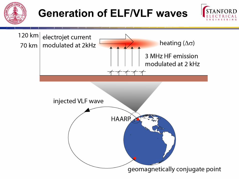
Generation of ELF/VLF waves

3

HAARP

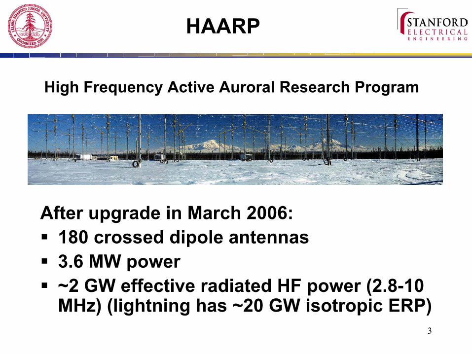
After upgrade in March 2006:180 crossed dipole antennas3.6 MW power~2 GW effective radiated HF power (2.8-10 MHz) (lightning has ~20 GW isotropic ERP)

High Frequency Active Auroral Research Program

4

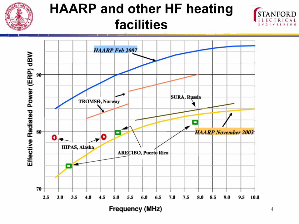
HAARP and other HF heating facilities

5

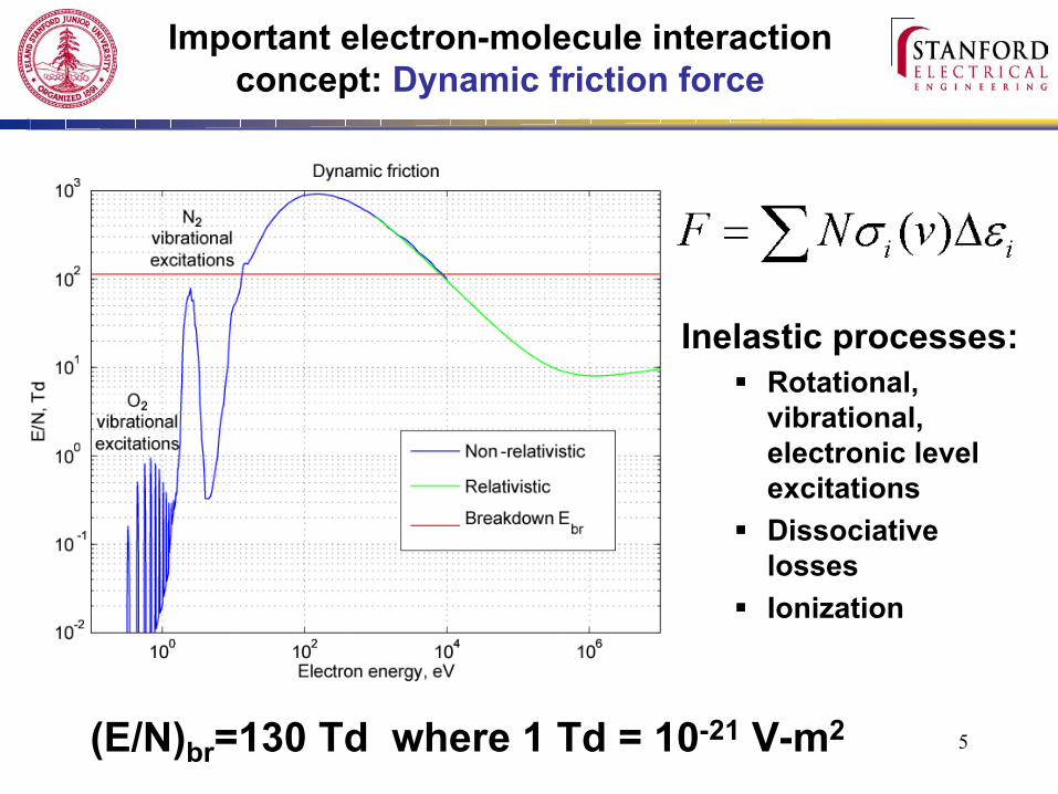
Important electron-molecule interaction concept: Dynamic friction force

Inelastic processes:Rotational, vibrational, electronic level excitationsDissociative lossesIonization

(E/N)br=130 Td where 1 Td = 10-21 V-m2

6

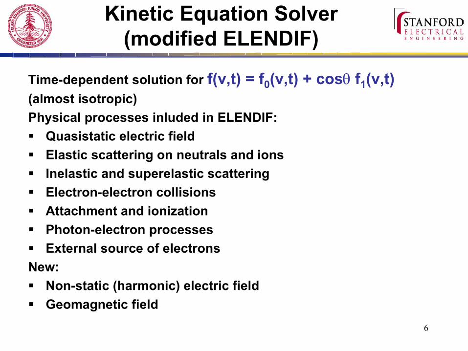
Kinetic Equation Solver(modified ELENDIF)

Time-dependent solution for f(v,t) = f0(v,t) + cosθ f1(v,t)(almost isotropic)Physical processes inluded in ELENDIF:

Quasistatic electric fieldElastic scattering on neutrals and ionsInelastic and superelastic scatteringElectron-electron collisionsAttachment and ionizationPhoton-electron processesExternal source of electrons

New:Non-static (harmonic) electric fieldGeomagnetic field

7

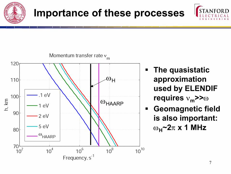
Importance of these processes

The quasistatic approximation used by ELENDIF requires νm>>ωGeomagnetic field is also important: ωH~2π x 1 MHz

ωH

ωHAARP

8

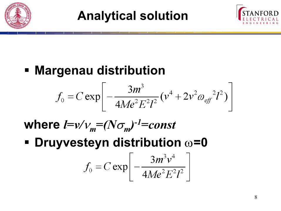
Analytical solution

Margenau distribution

where l=v/νm=(Nσm)-1=constDruyvesteyn distribution ω=0

9

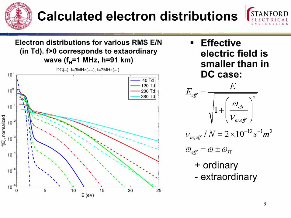
Calculated electron distributions

Electron distributions for various RMS E/N (in Td). f>0 corresponds to extaordinary

wave (fH=1 MHz, h=91 km)

Effective electric field is smaller than in DC case:

+ ordinary- extraordinary

10

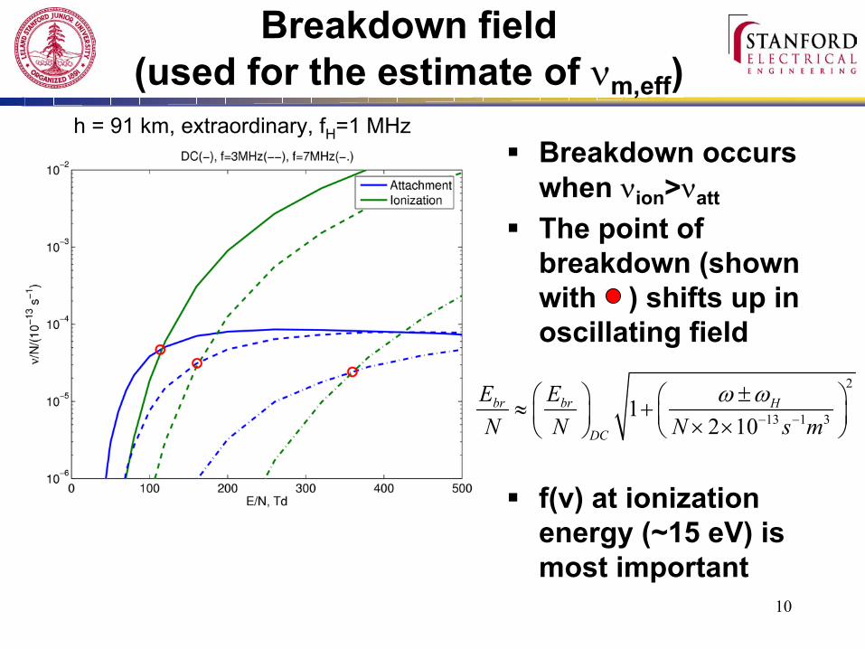
Breakdown field(used for the estimate of νm,eff)

Breakdown occurs when νion>νatt

The point of breakdown (shown with ) shifts up in oscillating field

f(v) at ionization energy (~15 eV) is most important

h = 91 km, extraordinary, fH=1 MHz

2

13 1 312 10

br br H

DC

E EN N N s m

ω ω− −

± ≈ + × ×

11

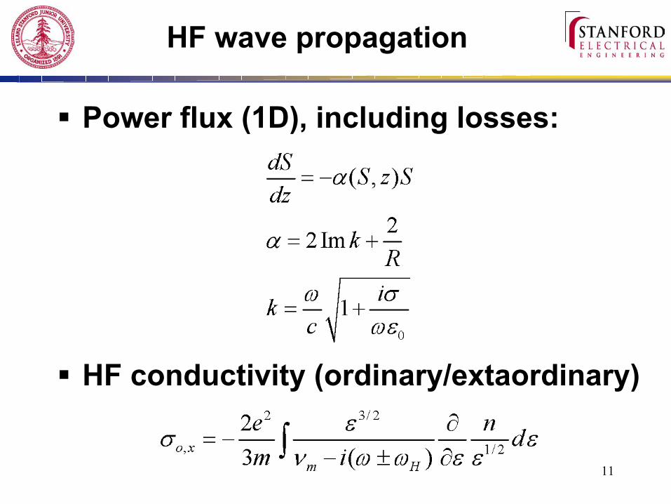
HF wave propagation

Power flux (1D), including losses:

HF conductivity (ordinary/extaordinary)

12

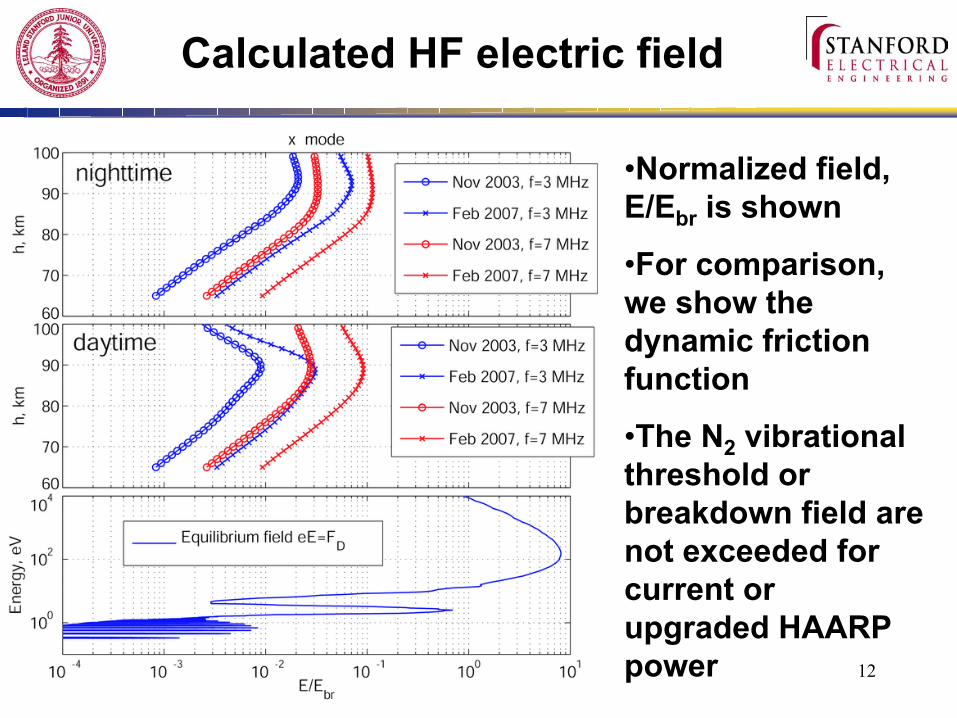
Calculated HF electric field

•Normalized field, E/Ebr is shown

•For comparison, we show the dynamic friction function

•The N2 vibrational threshold or breakdown field are not exceeded for current or upgraded HAARP power

13

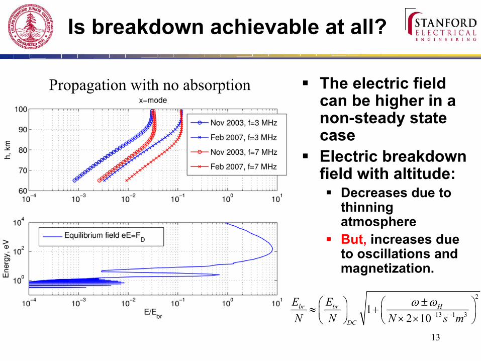
Is breakdown achievable at all?

The electric field can be higher in a non-steady state caseElectric breakdown field with altitude:

Decreases due to thinning atmosphereBut, increases due to oscillations and magnetization.

2

13 1 312 10

br br H

DC

E EN N N s m

ω ω− −

± ≈ + × ×

Propagation with no absorption

14

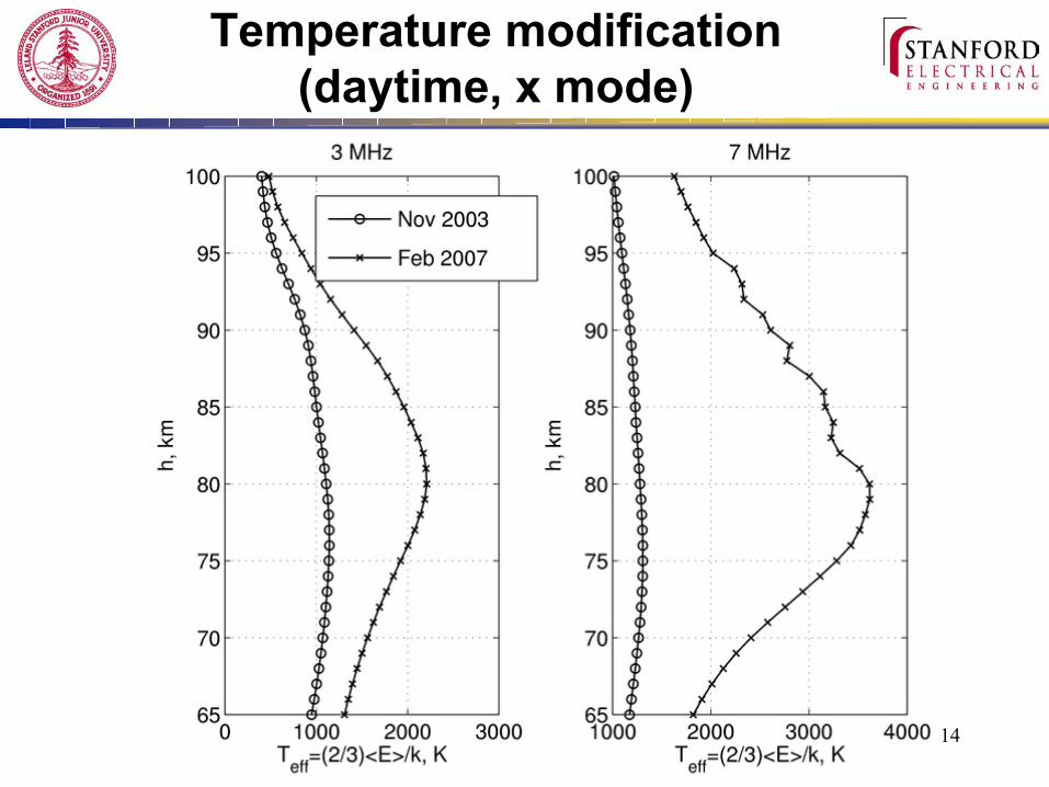
Temperature modification(daytime, x mode)

15

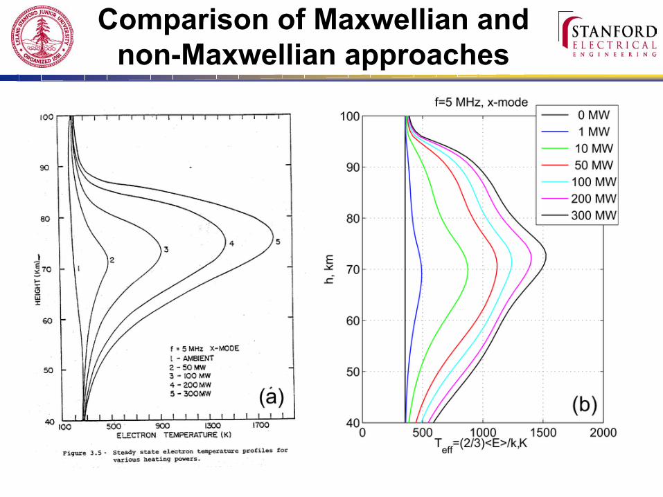
Comparison of Maxwellian andnon-Maxwellian approaches

16

DC conductivity changes(for electrojet current)

17

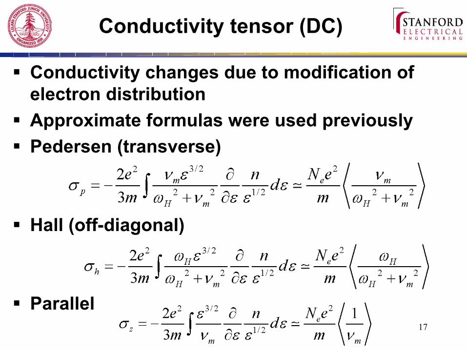
Conductivity tensor (DC)

Conductivity changes due to modification of electron distributionApproximate formulas were used previouslyPedersen (transverse)

Hall (off-diagonal)

Parallel

18

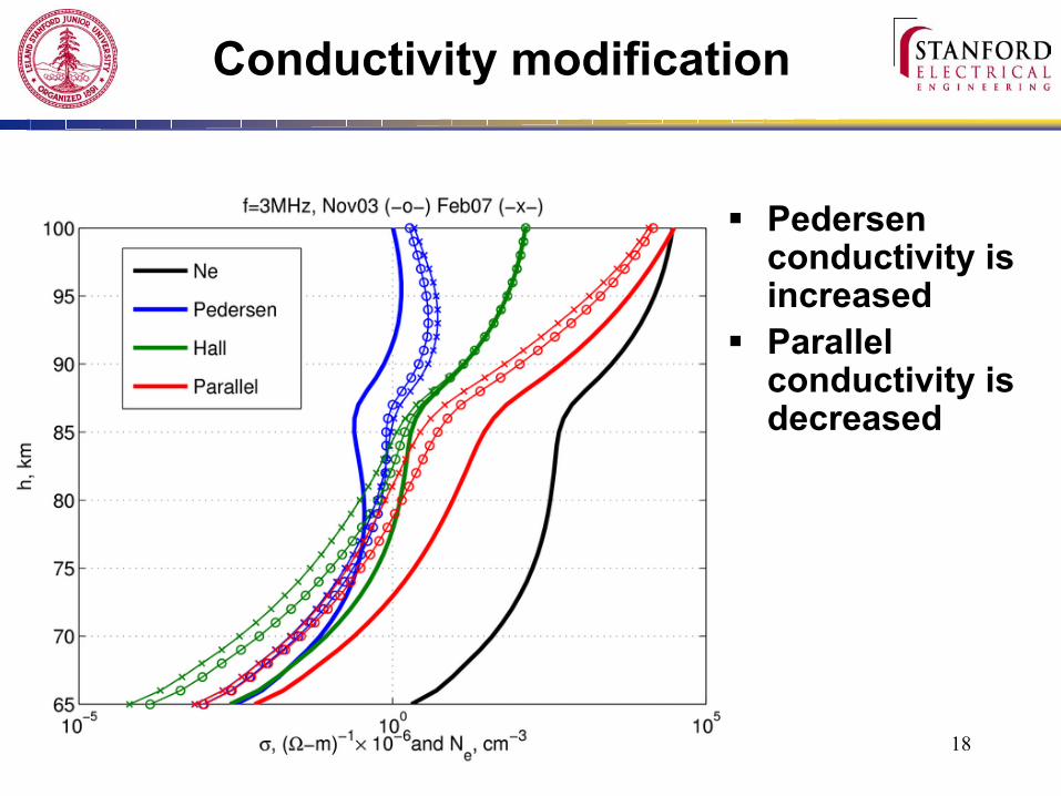
Conductivity modification

Pedersen conductivity is increasedParallel conductivity is decreased

19

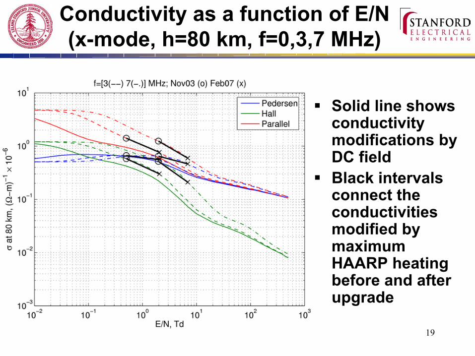
Conductivity as a function of E/N(x-mode, h=80 km, f=0,3,7 MHz)

Solid line shows conductivity modifications by DC fieldBlack intervals connect the conductivities modified by maximum HAARP heating before and after upgrade

20

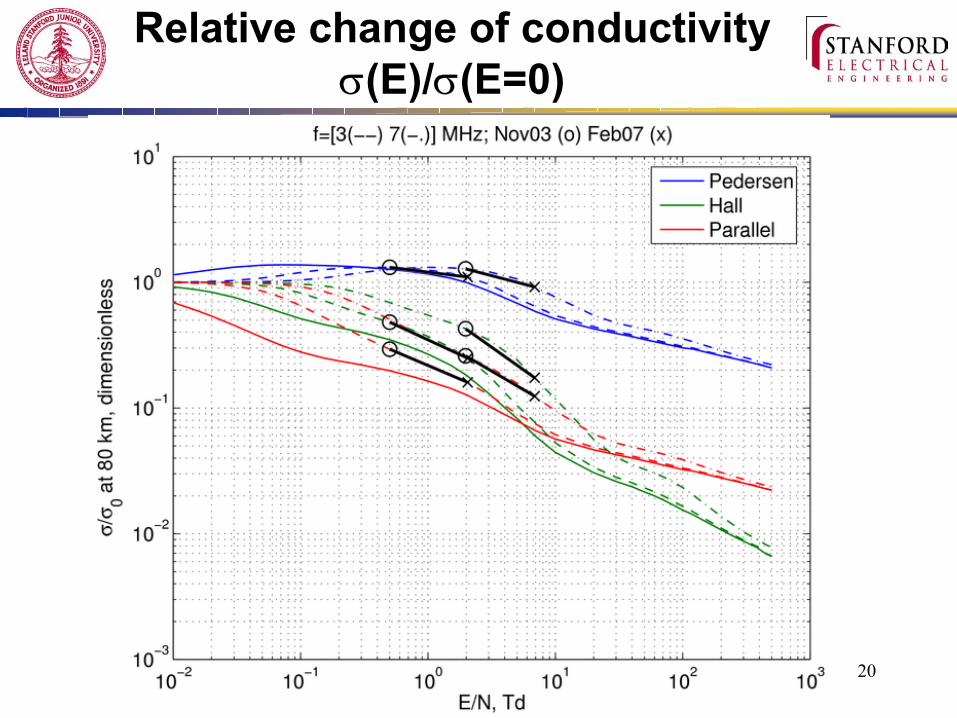
Relative change of conductivity σ(E)/σ(E=0)

21

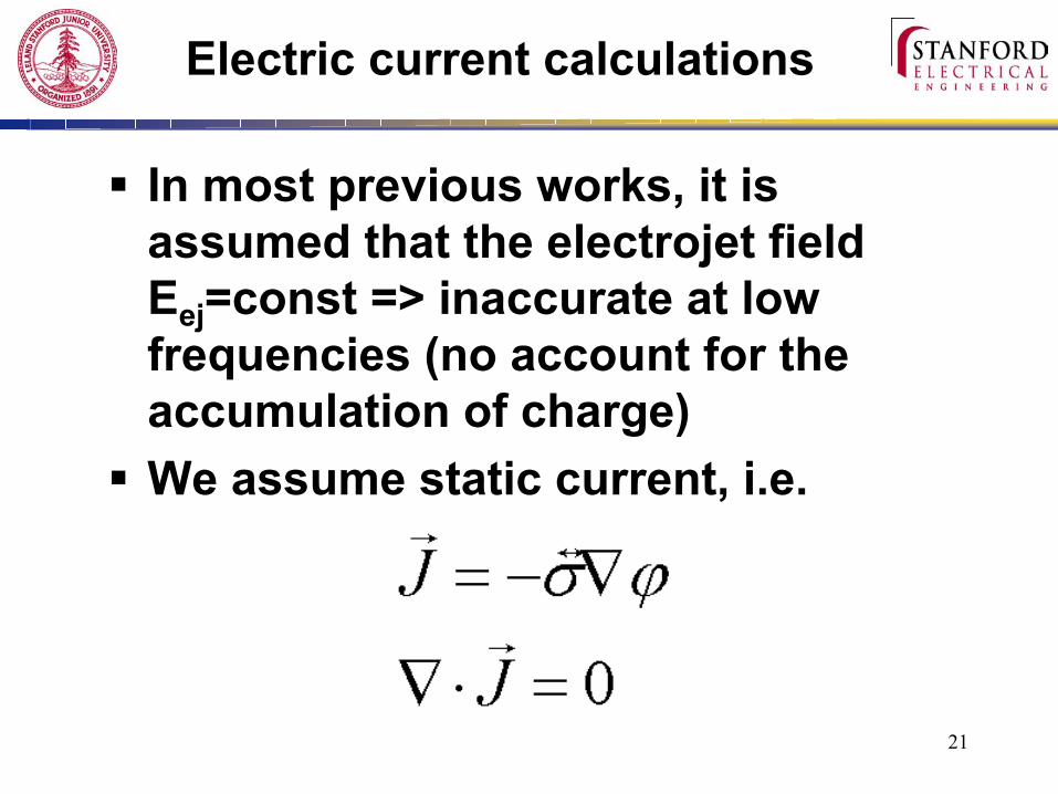
Electric current calculations

In most previous works, it is assumed that the electrojet field Eej=const => inaccurate at low frequencies (no account for the accumulation of charge)We assume static current, i.e.

22

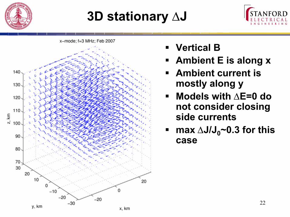
3D stationary ∆J

Vertical BAmbient E is along xAmbient current is mostly along yModels with ∆E=0 do not consider closing side currentsmax ∆J/J0~0.3 for this case

23

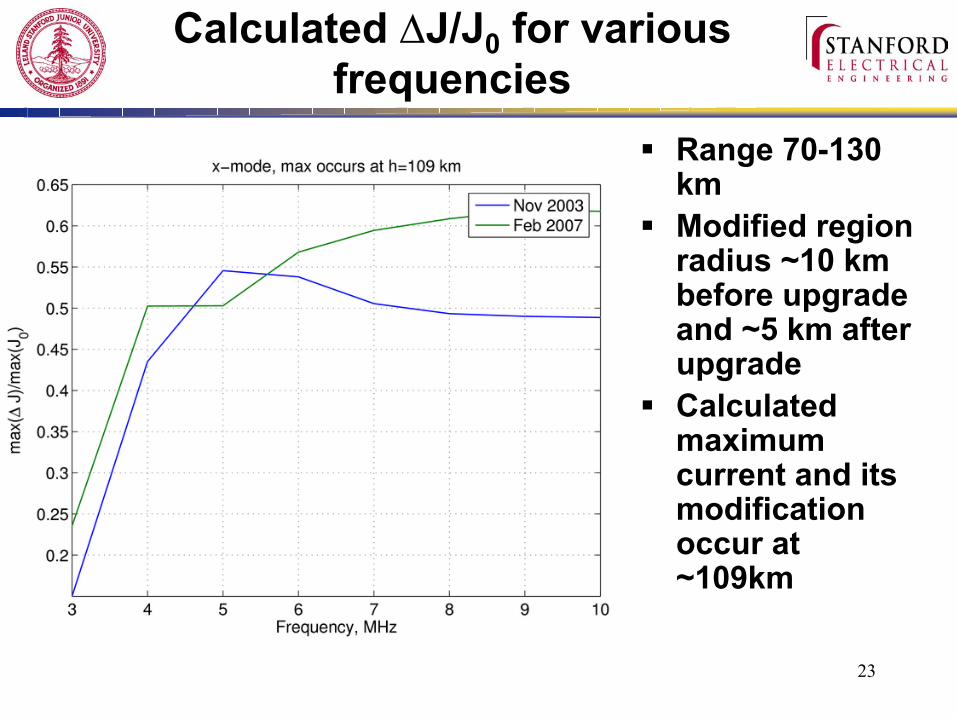
Calculated ∆J/J0 for various frequencies

Range 70-130 kmModified region radius ~10 km before upgrade and ~5 km after upgradeCalculated maximum current and its modification occur at ~109km

24

Conclusions

Our model includes both:Non-Maxwellian electron distributionSelf-absorption

Maxwellian electron distribution models, which calculate ∆Te, cannot account for the nonlinear Te saturation.The non-Maxwellian model allows to calculate processes for which high-energy tail of the electron distribution is important, such as:

optical emissionsbreakdown processes.

25

Work in progress

Electrojet current modulation in non-static caseELF/VLF emissionELF/VLF wave propagation along the geomagnetic field line