Recommendation ITU-R P.531-10(10/2009)

Ionospheric propagation data and prediction methods required for the design

of satellite services and systems

P Series

Radiowave propagation

ii Rec. ITU-R P.531-10

Foreword

The role of the Radiocommunication Sector is to ensure the rational, equitable, efficient and economical use of the radio-frequency spectrum by all radiocommunication services, including satellite services, and carry out studies without limit of frequency range on the basis of which Recommendations are adopted.

The regulatory and policy functions of the Radiocommunication Sector are performed by World and Regional Radiocommunication Conferences and Radiocommunication Assemblies supported by Study Groups.

Policy on Intellectual Property Right (IPR)

ITU-R policy on IPR is described in the Common Patent Policy for ITU-T/ITU-R/ISO/IEC referenced in Annex 1 of Resolution ITU-R 1. Forms to be used for the submission of patent statements and licensing declarations by patent holders are available from http://www.itu.int/ITU-R/go/patents/en where the Guidelines for Implementation of the Common Patent Policy for ITU-T/ITU-R/ISO/IEC and the ITU-R patent information database can also be found.

Series of ITU-R Recommendations (Also available online at http://www.itu.int/publ/R-REC/en)

Series Title

BO Satellite delivery BR Recording for production, archival and play-out; film for television BS Broadcasting service (sound) BT Broadcasting service (television) F Fixed service M Mobile, radiodetermination, amateur and related satellite services P Radiowave propagation RA Radio astronomy RS Remote sensing systems S Fixed-satellite service SA Space applications and meteorology SF Frequency sharing and coordination between fixed-satellite and fixed service systems SM Spectrum management SNG Satellite news gathering TF Time signals and frequency standards emissions V Vocabulary and related subjects

Note: This ITU-R Recommendation was approved in English under the procedure detailed in Resolution ITU-R 1.

Electronic Publication Geneva, 2009

© ITU 2009

All rights reserved. No part of this publication may be reproduced, by any means whatsoever, without written permission of ITU.

Rec. ITU-R P.531-10 1

RECOMMENDATION ITU-R P.531-10

Ionospheric propagation data and prediction methods required for the design of satellite services and systems

(Question ITU-R 218/3)

(1978-1990-1992-1994-1997-1999-2001-2003-2005-2007-2009)

Scope

Recommendation ITU-R P.531 describes a method for evaluating of the ionospheric propagation effects on Earth-space paths at frequencies from 0.1 to 12 GHz. The following effects may take place on an Earth-space path when the signal is passing through the ionosphere:

– rotation of the polarization (Faraday rotation) due to the interaction of the electromagnetic wave with the ionized medium in the Earth's magnetic field along the path;

– group delay and phase advance of the signal due to the total electron content (TEC) accumulated along the path;

– rapid variation of amplitude and phase (scintillations) of the signal due to small-scale irregular structures in the ionosphere;

– a change in the apparent direction of arrival due to refraction;

– Doppler effects due to non-linear polarization rotations and time delays.

The data and methods described in this Recommendation are applicable for planning satellite systems, in respective ranges of validity indicated in Annex 1.

The ITU Radiocommunication Assembly,

considering

a) that the ionosphere causes significant propagation effects at frequencies up to at least 12 GHz;

b) that effects may be particularly significant for non-geostationary-satellite orbit services below 3 GHz;

c) that experimental data have been presented and/or modelling methods have been developed that allow the prediction of the ionospheric propagation parameters needed in planning satellite systems;

d) that ionospheric effects may influence the design and performance of radio systems involving spacecraft;

e) that these data and methods have been found to be applicable, within the natural variability of propagation phenomena, for applications in satellite system planning,

recommends 1 that the data prepared and methods developed as set out in Annex 1 should be adopted for planning satellite systems, in the respective ranges of validity indicated in Annex 1.

2 Rec. ITU-R P.531-10

Annex 1

1 Introduction This annex deals with the ionospheric propagation effects on Earth-space paths. From a system design viewpoint, the impact of ionospheric effects can be summarized as follows: a) the total electron content (TEC) accumulated along a mobile-satellite service (MSS)

transmission path penetrating the ionosphere causes rotation of the polarization (Faraday rotation) of the MSS carrier, time delay of the signal, and a change in the apparent direction of arrival due to refraction;

b) localized random ionospheric patches, commonly referred to as ionospheric irregularities, further cause excess and random rotations and time delays, which can only be described in stochastic terms;

c) because the rotations and time delays relating to electron density are non-linearly frequency dependent, both a) and b) further result in dispersion or group velocity distortion of the MSS carriers;

d) furthermore, localized ionospheric irregularities also act like convergent and divergent lens which focus and defocus the radio waves. Such effects are commonly referred to as the scintillations which affect amplitude, phase and angle-of-arrival of the MSS signal.

Due to the complex nature of ionospheric physics, system parameters affected by ionospheric effects as noted above cannot always be succinctly summarized in simple analytic formulae. Relevant data edited in terms of tables and/or graphs, supplemented with further descriptive or qualifying statements, are for all practical purposes the best way to present the effects.

In considering propagation effects in the design of MSS at frequencies below 3 GHz, one has to recognize that: e) the normally known space-Earth propagation effects caused by hydrometeors are not

significant relative to effects of § f) and h); f) the near surface multipath effects, in the presence of natural or man-made obstacles and/or

at low elevation angles, are always critical; g) the near surface multipath effects vary from locality to locality, and therefore they do not

dominate the overall design of the MSS system when global scale propagation factors are to be dealt with;

h) ionospheric effects are the most significant propagation effects to be considered in the MSS system design in global scale considerations.

2 Background Caused by solar radiation, the Earth’s ionosphere consists of several regions of ionization. For all practical communications purposes, regions of the ionosphere, D, E, F and top-side ionization have been identified as contributing to the TEC between satellite and ground terminals.

In each region, the ionized medium is neither homogeneous in space nor stationary in time. Generally speaking, the background ionization has relatively regular diurnal, seasonal and 11-year solar cycle variations, and is dependent strongly on geographical locations and geomagnetic activity. In addition to the background ionization, there are always highly dynamic, small-scale non-stationary structures known as irregularities. Both the background ionization and irregularities degrade radiowaves. Furthermore, the refractive index is frequency dependent, i.e. the medium is dispersive.

Rec. ITU-R P.531-10 3

3 Prime degradations due to background ionizations A number of effects, such as refraction, dispersion and group delay, are in magnitude directly proportional to the TEC; Faraday rotation is also approximately proportional to TEC, with the contributions from different parts of the ray path weighted by the longitudinal component of magnetic field. A knowledge of the TEC thus enables many important ionospheric effects to be estimated quantitatively.

3.1 TEC Denoted as NT, the TEC can be evaluated by:

∫=s

eT ssnN d)( (1)

where: s : propagation path (m) ne : electron concentration (el/m3).

Even when the precise propagation path is known, the evaluation of NT is difficult because ne has diurnal, seasonal and solar cycle variations.

For modelling purposes, the TEC value is usually quoted for a zenith path having a cross-section of 1 m2. The TEC of this vertical column can vary between 1016 and 1018 el/m2 with the peak occurring during the sunlit portion of the day.

For estimating the TEC, either a procedure based on the international reference ionosphere (IRI) or a more flexible procedure, also suitable for slant TEC evaluation and based on NeQuick, are available. Both procedures are provided below.

3.1.1 IRI-based method The standard monthly median ionosphere is the COSPAR-URSI IRI-95. Under conditions of low to moderate solar activity numerical techniques may be used to derive values for any location, time and chosen set of heights up to 2 000 km. Under conditions of high solar activity, problems may arise with values of electron content derived from IRI-95. For many purposes it is sufficient to estimate electron content by multiplication of the peak electron density with an equivalent slab thickness value of 300 km.

3.1.2 NeQuick-based method The electron density distribution given by the model is represented by a continuous function that is also continuous in all spatial first derivatives. It consists of two parts, the bottom-side part (below the peak of the F2-layer) and the top-side part (above the F2-layer peak). The peak height of the F2-layer is calculated from M(3000)F2 and the ratio foF2/foE (see Recommen-dation ITU-R P.1239).

The bottom-side is described by semi-Epstein layers for representing E, F1 and F2. The top-side F layer is again a semi-Epstein layer with a height dependent thickness parameter. The NeQuick model gives the electron density and TEC along arbitrary ground-to-satellite or satellite-to-satellite paths.

The computer program and associated data files are available from the Radiocommunication Bureau.

4 Rec. ITU-R P.531-10

3.1.3 Model accuracy Estimates for the accuracy of the NeQuick and IRI models are given in documents published along with the trans-ionospheric propagation database on that part of the ITU-R website dealing with Radiocommunication Study Group 3.

3.2 Faraday rotation When propagating through the ionosphere, a linearly polarized wave will suffer a gradual rotation of its plane of polarization due to the presence of the geomagnetic field and the anisotropy of the plasma medium. The magnitude of Faraday rotation, θ, will depend on the frequency of the radiowave, the magnetic field strength, and the electron density of the plasma as:

2141036.2

fNB Tav−×=θ (2)

where: θ : angle of rotation (rad) Bav : average Earth magnetic field (Wb ⋅ m–2 or Teslas) f : frequency (GHz) NT : TEC (electrons ⋅ m–2).

Typical values of θ are shown in Fig. 1.

0531-01

102

1

10

103

104

10–1

10–2

1016

1017

1018

FIGURE 1Faraday rotation as a function of TEC and frequency

Frequency (GHz)

Fara

day

rota

tion

(rad)

1019 el/m2

1 0.1 0.2 0.5 2 5 100.3 0.4

The Faraday rotation is thus inversely proportional to the square of frequency and directly proportional to the integrated product of the electron density and the component of the Earth's magnetic field along the propagation path. Its median value at a given frequency exhibits a very regular diurnal, seasonal, and solar cyclical behaviour that can be predicted. This regular component of the Faraday rotation can therefore be compensated for by a manual adjustment of the polarization

Rec. ITU-R P.531-10 5

tilt angle at the earth-station antennas. However, large deviations from this regular behaviour can occur for small percentages of the time as a result of geomagnetic storms and, to a lesser extent, large-scale travelling ionospheric disturbances. These deviations cannot be predicted in advance. Intense and fast fluctuations of the Faraday rotation angles of VHF signals have been associated with strong and fast amplitude scintillations respectively, at locations situated near the crests of the equatorial anomaly.

The cross-polarization discrimination for aligned antennas, XPD (dB), is related to the Faraday rotation angle, θ, by:

XPD = –20 log (tan θ) (3)

3.3 Group delay The presence of charged particles in the ionosphere slows down the propagation of radio signals along the path. The time delay in excess of the propagation time in free space, commonly denoted as t, is called the group delay. It is an important factor to be considered for MSS systems. Likewise, the phase is advanced by the same amount. This quantity can be computed as follows:

t = 1.345 NT / f 2 × 10–7 (4)

where: t : delay time (s) with reference to propagation in a vacuum f : frequency of propagation (Hz) NT : determined along the slant propagation path.

Figure 2 is a plot of time delay, t, versus frequency, f, for several values of electron content along the ray path.

For a band of frequencies around 1 600 MHz the signal group delay varies from approximately 0.5 to 500 ns, for TEC from 1016 to 1019 el/m2. Figure 3 shows the yearly percentage of daytime hours that the time delay will exceed 20 ns at a period of relatively high solar activity.

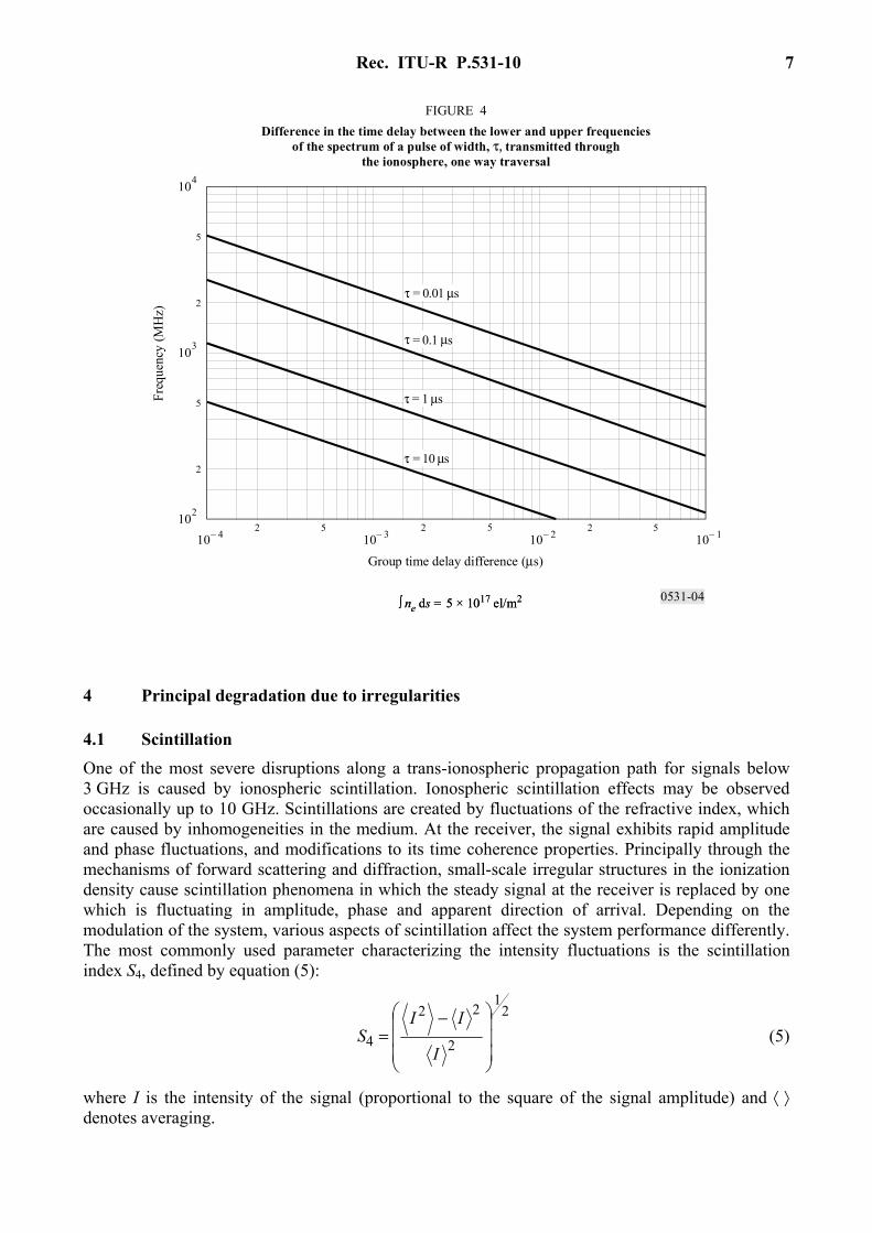
3.4 Dispersion When trans-ionospheric signals occupy a significant bandwidth the propagation delay (being a function of frequency) introduces dispersion. The differential delay across the bandwidth is proportional to the integrated electron density along the ray path. For a fixed bandwidth the relative dispersion is inversely proportional to frequency cubed. Thus, systems involving wideband transmissions must take this effect into account at VHF and possibly UHF. For example, as shown in Fig. 4 for an integrated electron content of 5 × 1017 el/m2, a signal with a pulse length of 1 μs will sustain a differential delay of 0.02 μs at 200 MHz while at 600 MHz the delay would be only 0.00074 μs (see Fig. 4).

3.5 TEC rate of change

With an orbiting satellite the observed rate of change of TEC is due in part to the change of direction of the ray path and in part to a change in the ionosphere itself. For a satellite at a height of 22 000 km traversing the auroral zone, a maximum rate of change of 0.7 × 1016 el/m2/s has been observed. For navigation purposes, such a rate of change corresponds to an apparent velocity of 0.11 m/s.

6 Rec. ITU-R P.531-10

0531-02

100 200 1 000500 2 000 3 000

102

10– 4

10– 3

10– 2

10– 1

1

10

2

5

2

5

2

5

2

5

2

5

2

5

1019

1016

1017

1018

l/m 2

FIGURE 2Ionospheric time delay versus frequency for various

values of electron contentIo

nosp

heric

tim

e de

lay

( μs)

Frequency (MHz)

e

FIGURE 3 Contours of percentage of yearly average daytime hours when time delay

at vertical incidence at 1.6 GHz exceeds 20 ns (sunspot number = 140)

0531-03

Latit

ude

Rec. ITU-R P.531-10 7

0531-04

τ = 1 μs

τ = 10 μs

2 5 2 5 2 510– 310– 4 10– 110– 2

2

5

102

2

5

103

104

FIGURE 4Difference in the time delay between the lower and upper frequencies

of the spectrum of a pulse of width, τ, transmitted throughthe ionosphere, one way traversal

Freq

uenc

y (M

Hz)

Group time delay difference (μs)

τ = 0.01 μs

τ = 0.1 μs

∫ ne ds = 5 × 1017 el/m2∫ ne ds = 5 × 1017 el/m2

4 Principal degradation due to irregularities

4.1 Scintillation

One of the most severe disruptions along a trans-ionospheric propagation path for signals below 3 GHz is caused by ionospheric scintillation. Ionospheric scintillation effects may be observed occasionally up to 10 GHz. Scintillations are created by fluctuations of the refractive index, which are caused by inhomogeneities in the medium. At the receiver, the signal exhibits rapid amplitude and phase fluctuations, and modifications to its time coherence properties. Principally through the mechanisms of forward scattering and diffraction, small-scale irregular structures in the ionization density cause scintillation phenomena in which the steady signal at the receiver is replaced by one which is fluctuating in amplitude, phase and apparent direction of arrival. Depending on the modulation of the system, various aspects of scintillation affect the system performance differently. The most commonly used parameter characterizing the intensity fluctuations is the scintillation index S4, defined by equation (5):

2

1

2

22

4⎟⎟⎟

⎠

⎞

⎜⎜⎜

⎝

⎛ −=

I

IIS (5)

where I is the intensity of the signal (proportional to the square of the signal amplitude) and ⟨ ⟩ denotes averaging.

8 Rec. ITU-R P.531-10

The scintillation index S4 is related to the peak-to-peak fluctuations of the intensity. The exact relationship depends on the distribution of the intensity. The intensity distribution is best described by the Nakagami distribution for a wide range of S4 values.

Scintillation strength may, for convenience, be classified into three regimes: weak, moderate or strong. The weak values correspond to S4 < 0.3, the moderate values from 0.3 to 0.6 and the strong case for S4 > 0.6.

For weak and moderate regimes, S4 shows a consistent f –υ frequency dependence, with υ being 1.5

for most multifrequency observations. In addition for weak regimes the amplitude follows a log-normal distribution.

In the strong regime, it has been observed that the υ factor decreases. This is due to the saturation of scintillation under the strong influence of multiple scattering. As S4 approaches 1.0, the intensity follows a Rayleigh distribution. Occasionally, S4 may exceed 1, reaching values as high as 1.5. Figure 5 shows an example of the frequency dependence of S4 at VHF and UHF for three auroral stations for weak, moderate and strong scintillations.

The phase scintillations follow a Gaussian distribution with zero mean. The standard deviation is used to characterize the phase scintillations (σφ). For weak and moderate regimes, most observations in equatorial regions indicate that phase and intensity scintillation are strongly correlated; S4 and σφ (when expressed in radians) have similar values.

FIGURE 5 Scintillation indices measured at Kiruna (a), Lulea (b), and Kokkola (c) at 150 MHz

(dotted line) and 400 MHz (dashed line), as recorded from polar orbiting LEO Tsykada satellites during disturbed conditions on 30 October 2003

0531-05

1.5

1

0.5

021:26:41 21:30:41 21:34:41 21:38:41 21:42:41

1.5

1

0.5

023:11:39 23:15:39 23:19:39 23:23:39 23:27:39

1.5

1

0.5

019:28:59 19:32:59 19:36:59 19:40:59 19:44:59

UT

S 4

Rec. ITU-R P.531-10 9

Empirically, Table 1 provides a convenient conversion between S4 and the approximate peak-to-peak fluctuations Pfluc (dB). This relationship can be approximated by:

Pfluc = 27.5 S41.26 (6)

TABLE 1

Empirical conversion table for scintillation indices

S4 Pfluc (dB)

0.1 1.5 0.2 3.5 0.3 6 0.4 8.5 0.5 11 0.6 14 0.7 17 0.8 20 0.9 24 1.0 27.5

4.2 Geographic, seasonal and solar dependence of scintillations Geographically, there are two intense zones of scintillation, one at high latitudes and the other centred within ± 20° of the magnetic equator as shown in Fig. 6. Severe scintillation has been observed up to gigahertz frequencies in these two sectors, while in the middle latitudes scintillation occurs exceptionally, such as during geomagnetic storms. In the equatorial sector, there is a pronounced night-time maximum of activity as also indicated in Figs. 6 and 7. For equatorial gigahertz scintillation, peak activity around the vernal equinox and high activity at the autumnal equinox have been observed.

A typical scintillation event has its on-set after local ionospheric sunset and an event can last from 30 min to hours. For equatorial stations in years of solar maximum, ionospheric scintillation occurs almost every evening after sunset, with the peak-to-peak fluctuations of signal level at 4 GHz exceeding 10 dB in magnitude.

4.3 Ionospheric scintillation model In order to predict the intensity of ionospheric scintillation on Earth-space paths, it is recommended that the global ionospheric scintillation model (GISM) be used. The GISM permits one to predict the S4 index, the depth of amplitude fading as well as the rms phase and angular deviations due to scintillation as a function of satellite and ground station locations, date, time and working frequency. The model is based on the multiple phase screen method. The main internal parameters of the model are set to the following default values: − Slope of the intensity spectrum, p = 3 − Average size of the irregularities, L0 = 500 km − Standard deviation of the electron density fluctuations, σNe = 0.2.

10 Rec. ITU-R P.531-10

The bending of the rays is taken into account and the characteristics of the background ionosphere are computed in a sub-routine which uses the NeQuick ionospheric model. The source code of the GISM is available on that part of the ITU-R website related to Radiocommunication Study Group 3, along with the relevant documentation.

4.4 Instantaneous statistics and spectrum behaviour

4.4.1 Instantaneous statistics During an ionospheric scintillation event, the Nakagami density function is believed to be adequately close for describing the statistics of the instantaneous variation of amplitude. The density function for the intensity of the signal is given by:

)(–exp)(

)( 1– mIIm

mIp mm

Γ= (7)

FIGURE 6 Depth of scintillation fading (proportional to density of cross-hatching)

at 1.5 GHz during solar maximum and minimum years

0531-06

Mid

nigh

t

Mid

nigh

t

10 dB

FIGURE 7 Distribution of one year scintillation events at Cayenne during June 06 to July 07; S4 level

weak (top); moderate (middle); strong (bottom) for elevation angles > 20°

0531-07Hour (HL)

Even

t num

ber

12 16 420 24 8 12

400

300

200

100

0

All the year

Cayenne: data from June 06 to July 07 level: (0.25-0.4), (0.4, 0, 0.55), (>0.55)

Elavation > 20º, after multipath correctionS4

Local time

Rec. ITU-R P.531-10 11

where the Nakagami “m-coefficient” is related to the scintillation index, S4 by:

42/1 Sm = (8)

In formulating equation (7) the average intensity level of I is normalized to be 1.0. The calculation of the fraction of time that the signal is above or below a given threshold is greatly facilitated by the fact that the distribution function corresponding to the Nakagami density has a closed form expression which is given by:

∫ ΓΓ==

I

mmImxxpIP

0 )(),(d)()( (9)

where Γ(m, mI ) and Γ(m) are the incomplete gamma function and gamma function, respectively. Using equation (9), it is possible to compute the fraction of time that the signal is above or below a given threshold during an ionospheric event. For example, the fraction of time that the signal is more than X dB below the mean is given by P (10 –X / 10) and the fraction of time that the signal is more than Y dB above the mean is given by 1 – P(10Y / 10).

4.4.2 Spectrum behaviour In terms of temporal characteristics, the fading rate of ionospheric scintillation is about 0.1 to 1 Hz. The spatial and temporal power spectra exhibit a wide range of slopes, from f

–1 to f –6 as have been

reported from different observations. A typical spectrum behaviour is shown in Fig. 8. The f –3 slope

as shown is recommended for system applications if direct measurement results are not available. This value is representative of weak to moderate scintillation events.

The roll-off frequency differs from amplitude and phase scintillation as shown in Fig. 9. Phase scintillation presents more pronounced low frequency components than amplitude scintillation.

4.5 Geometric consideration

4.5.1 Zenith angle dependence

In most models, 42S is shown to be proportional to the secant of the zenith angle, i, of the

propagation path. This relationship is believed to be valid up to i ≈ 70° for weak and moderate scintillation levels. At greater zenith angles, a dependence ranging between 1/2 and first power of sec i should be used.

4.5.2 Seasonal-longitudinal dependence The occurrence of scintillations and magnitude of S4 have a longitudinal as well as seasonal dependence that can be parameterized by the angle, β, shown in Fig. 9b. It is the angle between the sunset terminator and local magnetic meridian at the apex of the field line passing through the line-of-sight at the height of the irregularity slab. The weighting function for seasonal-longitudinal dependence is given by:

⎥⎦⎤

⎢⎣⎡ β−∝

WS exp4 (10)

where W is a weighting constant depending on location as well as calendar day of the year. As an example, using the data available from Tangua, Hong Kong and Kwajalein, the numerical value of the weighting constant can be modelled as shown in Fig. 10.

12 Rec. ITU-R P.531-10

0531-08

FIGURE 8Power spectral density estimates for a geostationary satellite (Intelsat-IV) at 4 GHz

Rel

ativ

e po

wer

spec

tral d

ensit

y (d

B)

Fluctuation frequency (Hz)

The scintillation event was observed during the eveningsof 28-29 April 1977 at Taipei earth station

A:B:C:D:E:F:

30 min before event onsetat the beginning1 h after2 h after3 h after4 h after

Signal fluctuation28-29 April 1977

10 10

D

Rec. ITU-R P.531-10 13

FIGURE 9 Typical intensity and phase spectrum

0531-09

Power densities

Frequency (Hz)

0.01 0.1 1 10 1001.10–3

1.10–3

1.103

100

10

1

0.1

0.01

1.10–4

1.10–5

1.10–6

Amplitude

Phase

0531-09a

FIGURE 9aIntersection of the propagation path with a magnetic field line at the F-region height

Apex of field line

14 Rec. ITU-R P.531-10

FIGURE 9b Angle between the local magnetic meridian at the apex of the field line

shown in Fig. 9a and the sunset terminator

0531-09b

Sunset terminator

Magneticmeridian

Apex of field line

0531-10

FIGURE 10Seasonal weighting functions for stations in different longitude sectors

Tangua (22° 44 S, 42° 43 W)' '

Kwajalein(09° 05 N, 167° 20 E)' '

(22° 16 N, 114° 09 E)' '

Rec. ITU-R P.531-10 15

4.6 Cumulative statistics When considering the design of satellite radiocommunication systems and the assessment of frequency sharing, communications engineers have concerns not only with the system degradation and interference during an event but also with the long-term cumulative occurrence statistics. For communications systems involving a geostationary satellite, which is the simplest radio system configuration, Figs. 11 and 12 are recommended for the assessment and scaling of occurrence statistics. The sunspot numbers cited are the 12 month averaged sunspot numbers.

The long-term cumulative distribution, P(I), of the signal intensity relative to its mean value can be derived from the long-term cumulative statistics, F(ξ), of the peak-to-peak fluctuation, ξ, such as those found in Fig. 11, as follows:

∑=

=n

iii IPfIP

0)( )( (11)

where:

f0 = F (ξ < ξ1) (11a)

fi = F (ξi ≤ ξ < ξi + 1) (i = 1, 2, …, n – 1) (11b)

fn = F (ξ ≥ ξn ) (11c)

and ξ1 and ξn are the minimum and maximum peak-to-peak fluctuation values, respectively, and n is the interval number of ξ of interest to the user:

Pi(I) = Γ (mi, miI) / Γ(mi) (11d)

241/ ii Sm = (11e)

26.1/1

140 25.27

1⎥⎦⎤

⎢⎣⎡ ξ⋅=S (11f)

26.1/1

14 25.27

1⎥⎦

⎤⎢⎣

⎡ ξ+ξ⋅= +ii

iS (i = 1, 2, … n – 1) (11g)

26.1/1

14 4

35.27

1⎥⎦

⎤⎢⎣

⎡ ξ+ξ⋅= − nn

nS (11h)

Figure 12 shows an example of long-term cumulative distribution of signal intensity derived from the curve P6 of Fig. 11.

4.7 Simultaneous occurrence of ionospheric scintillation and rain fading Ionospheric scintillation and rain fading are two impairments of completely different physical origin. However, in equatorial regions at years of high sunspot number, the simultaneous occurrence of the two effects may have an annual percentage time that is significant to system design. The cumulative simultaneous occurrence time was about 0.06% annually as noted at 4 GHz at Djutiluhar earth station in Indonesia.

The simultaneous events have signatures that are often vastly different from those when only a single impairment, either scintillation or rain alone, is present. While ionospheric scintillation alone is not a depolarization phenomenon, and rain fading alone is not a signal fluctuation phenomenon (although it may cause slight fluctuations of polarization for moderate to strong scintillations), the simultaneous events produce a significant amount of signal fluctuations in the cross-polarization

16 Rec. ITU-R P.531-10

channel. Recognition of these simultaneous events is needed for applications to satellite-Earth radio systems which require high availability.

The prediction of rain fading is described in Recommendation ITU-R P.618.

FIGURE 11 Dependence of 4 GHz equatorial ionospheric scintillations

on monthly mean sunspot number

0531-11

Perc

enta

ge o

f tim

e in

a y

ear t

hat p

eak-

to-p

eak

fluct

uatio

n ex

ceed

s 1 d

B

Monthly sunspot numbers

The squares are the ranges of variations over a yearfor different carriers

A:B:C:D:E:F:G:

1975-1976, Hong Kong and Bahrein, 15 carriers1974, Longovilo, 1 carrier1976-1977, Taipei, 2 carriers1970-1971, 12 stations, > 50 carriers1977-1978, Hong Kong, 12 carriers1978-1979, Hong Kong, 10 carriers1979-1980, Hong Kong, 6 carriers

D

4.8 Gigahertz scintillation model To evaluate the scintillation effects that can be expected in a given situation the following steps may be used:

Step 1: Figure 12 provides scintillation occurrence statistics on equatorial ionospheric paths: peak-to-peak amplitude fluctuations, Pfluc, (dB), for 4 GHz reception from satellites in the East at elevation angles of about 20° (P solid curves) and in the West at about 30° elevation (I dotted curves). The data are given for different times of year and sunspot number.

Rec. ITU-R P.531-10 17

Step 2: Since Fig. 12 relates to 4 GHz, values for other frequencies are found by multiplying these values by ( f /4)–1.5 where f is the frequency of interest (GHz).

Step 3: The variation of Pfluc with geographical location and diurnal occurrence can be qualitatively estimated from Fig. 5.

Step 4: As one element of link budget calculations, Pfluc is related to signal loss Lp by .2/flucp PL =

Step 5: The scintillation index S4, the most widely used parameter in describing scintillation, is defined in § 4.1 and may be obtained from Pfluc using Table 1.

FIGURE 12 Annual statistics of peak-to-peak fluctuations observed at

Hong Kong earth station (Curves I1, P1, I3-I6, P3-P6) and Taipei earth station (Curves P2 and I2)

0531-12

Peak-to-peak fluctuation (dB)

CurveI1, P1I2, P2I3, P3I4, P4I5, P5I6, P6

PeriodMarch 75-76June 76-77March 77-78October 77-78November 78-79June 79-80

18 Rec. ITU-R P.531-10

0531-13

2

1

0

–1

–2

–3

–4

1 2 5 10 20 30 40 50 60 70 80 90 95 98 99

FIGURE 13An example of long-term cumulative statistics of signal intensity (4 GHz, 20° elevation)

Percentage of time the ordinate is not exceeded

Sign

al in

tens

ity (d

B)

99.5 99.9999.999.80.01 0.1 0.50.2

5 Absorption When direct information is not available, ionospheric absorption loss can be estimated from available models according to the (sec i ) / f 2 relationship for frequencies above 30 MHz, where i is the zenith angle of the propagation path in the ionosphere. For equatorial and mid-latitude regions, radiowaves of frequencies above 70 MHz will assure penetration of the ionosphere without significant absorption.

Measurements at middle latitudes indicate that, for a one-way traverse of the ionosphere at vertical incidence, the absorption at 30 MHz under normal conditions is typically 0.2 to 0.5 dB. During a solar flare, the absorption will increase but will be less than 5 dB. Enhanced absorption can occur at high latitudes due to polar cap and auroral events; these two phenomena occur at random intervals, last for different periods of time, and their effects are functions of the locations of the terminals and the elevation angle of the path. Therefore for the most effective system design these phenomena should be treated statistically bearing in mind that the durations for auroral absorption are of the order of hours and for polar cap absorption are of the order of days.

Rec. ITU-R P.531-10 19

5.1 Auroral absorption Auroral absorption results from increases of electron concentration in the D and E regions produced by incident energetic electrons. The absorption is observed over a range of 10° to 20° latitude centred close to the latitude of maximum occurrence of visual aurorae. It occurs as a series of discrete absorption enhancements each of relatively short duration, i.e. from minutes up to a few hours, with an average duration of about 30 min, and usually showing an irregular time structure. Night enhancements tend to consist of smooth fast rises and slow decays. Typical magnitudes at 127 MHz are shown in Table 2.

TABLE 2

Auroral absorption at 127 MHz (dB)

Angle of elevation Percentage of the time 20° 5°

0.1 1.5 2.9 1 0.9 1.7 2 0.7 1.4 5 0.6 1.1

50 0.2 0.4

5.2 Polar cap absorption Polar cap absorption which may occur at times of high solar activity, does so at geomagnetic latitudes greater than 64°. The absorption is produced by ionization at heights greater than about 30 km. It usually occurs in discrete, though sometimes overlapping, events which are nearly always associated with discrete solar events. The absorption is long-lasting and is detectable over the sunlit polar caps. Polar cap absorption occurs most usually during the peak of the sunspot cycle, when there may be 10 to 12 events per year. Such an event may last up to a few days. This is in contrast to auroral absorption, which is frequently quite localized, with variations in periods of minutes.

A remarkable feature of a polar cap absorption event is the great reduction in the absorption during hours of darkness for a given rate of electron production. Figure 14 is a hypothetical model of the diurnal variation of polar cap absorption following a major solar flare based upon riometer observations at various latitudes.

20 Rec. ITU-R P.531-10

FIGURE 14 Hypothetical model showing polar cap absorption following a major solar flare

as expected to be observed on riometers at approximately 30 MHz

0531-14

Abs

orpt

ion

(dB)

A:B:C:

high latitudes – 24 h of daylighthigh latitudes – equal period of day and nighthigh latitudes – auroral zone

6 Summary Table 3 estimates maximum values for ionospheric effects at a frequency of 1 GHz. It is assumed that the total vertical electron content of the ionosphere is 1018 el/m2 column. An elevation angle of about 30° is also assumed. The values given are for the one-way traversal of the waves through the ionosphere.

Rec. ITU-R P.531-10 21

TABLE 3

Estimated maximum ionospheric effects at 1 GHz for elevation angles of about 30° one-way traversal

Effect Magnitude Frequency dependence

Faraday rotation 108° 1/f 2 Propagation delay 0.25 μs 1/f 2 Refraction < 0.17 mrad 1/f 2 Variation in the direction of arrival

0.2 min of arc 1/f 2

Absorption (polar cap absorption) 0.04 dB ∼1/f 2 Absorption (auroral + polar cap absorption) 0.05 dB ∼1/f 2 Absorption (mid-latitude) < 0.01 dB 1/f 2 Dispersion 0-4 ns/MHz 1/f 3 Scintillation See § 4 See § 4