UNEP PNUE WMO OMM INTERGOVERNMENTAL PANEL ON CLIMATE CHANGE IPCC Technical Paper III STABILIZATION OF ATMOSPHERIC GREENHOUSE GASES: PHYSICAL, BIOLOGICAL AND SOCIO-ECONOMIC IMPLICATIONS m a t e o b je c t o f t h is C o n v e n ti o n and a n y rel at ed l eg c e o f t h e p a r ti e s m a y a d o p t is to achieve, i n acc o r d a ns o f t h e C o n v e n ti o n , s t a b iliz a tion of greenho u s e g a ere a t a le v e l t h a t w o u l d p r e v e n t dangerous ant h r o p sys t e m . S u c h a le v e l s h o u ld b e achieved withi n a t i m ns t o a d a p t n a t u r a ll y t o c li m a t e change, to ensu r e t h d a n d t o e n a b le e c o n o m ic d e v elo p m ent to proc e e d i n
Transcript
UNEP
PNUE
WMO
OMM
INTERGOVERNMENTAL PANEL ON CLIMATE CHANGE
IPCC Technical Paper III
STABILIZATION OF ATMOSPHERICGREENHOUSE GASES:
PHYSICAL, BIOLOGICAL AND SOCIO-ECONOMIC IMPLICATIONS
mate object of this Convention and any related leg
ce of the parties may adopt is to achieve, in accorda
ns of the Convention, stabilization of greenhouse ga
ere at a level that would prevent dangerous anthrop
system. Such a level should be achieved within a tim
ns to adapt naturally to climate change, to ensure th
d and to enable economic development to proceed in
Stabilization of Atmospheric Greenhouse Gases:
Physical, Biological and Socio-economic
Implications
Edited by
John T. Houghton L. Gylvan Meira Filho David J. Griggs Kathy Maskell
February 1997
This paper was prepared under the auspices of IPCC Working Group I, which is co-chaired by Sir John T. Houghton of the United Kingdom and Dr L. Gylvan Meira Filho of Brazil.
UNEP
PNUE
WMO
OMM
INTERGOVERNMENTAL PANEL ON CLIMATE CHANGE
This is a Technical Paper of the Intergovernmental Panel on Climate Change prepared in response to a requestfrom the United Nations Framework Convention on Climate Change. The material herein has undergone expertand government review, but has not been considered by the Panel for possible acceptance or approval.
1.2.2 Stabilization of CO2 Concentrations (see SAR WGI for more details) . . . . . . . . . . . . . . . . . . . . . . . 81.2.3 Taking the Climatic Effects of Other Greenhouse Gases and Aerosols into Account: the Concept of
This Intergovernmental Panel on Climate Change (IPCC)Technical Paper on “Stabilization of Atmospheric GreenhouseGases: Physical, Biological and Socio-economic Implications”is the third paper in the IPCC Technical Paper series and wasproduced in response to a request made by the Subsidiary Bodyfor Scientific and Technological Advice (SBSTA) of theConference of the Parties (COP) to the United NationsFramework Convention on Climate Change (UN/FCCC).
Technical Papers are initiated either at the request of the bodiesof the COP, and agreed by the IPCC Bureau, or as decided bythe IPCC. They are based on the material already in IPCCAssessment Reports and Special Reports and are written byLead Authors chosen for the purpose. They undergo a simulta-neous expert and government review, during which commentson this Paper were received from 93 reviewers from 27 coun-tries, followed by a final government review. The Bureau of theIPCC acts in the capacity of an editorial board to ensure thatreview comments have been adequately addressed by the LeadAuthors in the finalization of the Technical Paper.
The Bureau met in its Twelfth Session (Geneva, 3-5 February1997) and considered the major comments received during thefinal government review. In the light of its observations andrequests, the Lead Authors finalized the Technical Paper. TheBureau was satisfied that the agreed Procedures had beenfollowed and authorized the release of the Paper to the SBSTAand thereafter publicly.
We owe a large debt of gratitude to the Lead Authors who gaveof their time very generously and who completed the Paper atshort notice and according to schedule. We thank the Co-chairmen of Working Group I of the IPCC, John Houghton andGylvan Meira Filho who oversaw the effort, the staff of theUnited Kingdom Meteorological Office graphics studio whoprepared the figures for publication, Christy Tidd who assistedthe convening Lead Author in the preparation of the paper andparticularly David Griggs, Kathy Maskell and Anne Murrillfrom the IPCC Working Group I Technical Support Unit, fortheir insistence on adhering to quality and timeliness.
B. Bolin N. SundararamanChairman of the IPCC Secretary of the IPCC
Stabilization of Atmospheric Greenhouse Gases: Physical, Biological and Socio-economic Implicationsvi
Stabilization of Atmospheric GreenhouseGases: Physical, Biological and Socio-economic ImplicationsThis paper was prepared under the auspices of IPCC Working Group I.
Lead Authors:David Schimel, Michael Grubb, Fortunat Joos, Robert Kaufmann, Richard Moss, Wandera Ogana,Richard Richels, Tom Wigley
Contributors:Regina Cannon, James Edmonds, Erik Haites, Danny Harvey, Atul Jain, Rik Leemans, Kathleen Miller,Robert Parkin, Elizabeth Sulzman, Richard van Tol, Jan de Wolde
Modellers:Michele Bruno, Fortunat Joos, Tom Wigley
Introduction
An understanding of the constraints on the stabilization ofgreenhouse gas concentrations is fundamental to policy formu-lation with regard to the goals of the United Nations FrameworkConvention on Climate Change and its implementation. ThisTechnical Paper provides:
(a) A tutorial on the stabilization of greenhouse gases, the esti-mation of radiative forcing1, and the concept of “equivalentcarbon dioxide (CO2)” (the concentration of CO2 that leadsto global mean radiative forcing consistent with projectedincreases in all gases when a suite of gases is being consid-ered);
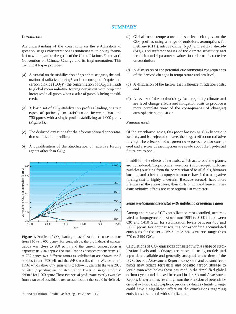
(b) A basic set of CO2 stabilization profiles leading, via twotypes of pathway, to stabilization between 350 and750 ppmv, with a single profile stabilizing at 1 000 ppmv(Figure 1);
(c) The deduced emissions for the aforementioned concentra-tion stabilization profiles;
(d) A consideration of the stabilization of radiative forcingagents other than CO2;
(e) Global mean temperature and sea level changes for theCO2 profiles using a range of emissions assumptions formethane (CH4), nitrous oxide (N2O) and sulphur dioxide(SO2), and different values of the climate sensitivity andice-melt model parameter values in order to characterizeuncertainties;
(f) A discussion of the potential environmental consequencesof the derived changes in temperature and sea level;
(g) A discussion of the factors that influence mitigation costs;and
(h) A review of the methodology for integrating climate andsea level change effects and mitigation costs to produce amore complete view of the consequences of changingatmospheric composition.
Fundamentals
Of the greenhouse gases, this paper focuses on CO2 because ithas had, and is projected to have, the largest effect on radiativeforcing. The effects of other greenhouse gases are also consid-ered and a series of assumptions are made about their potentialfuture emissions.
In addition, the effects of aerosols, which act to cool the planet,are considered. Tropospheric aerosols (microscopic airborneparticles) resulting from the combustion of fossil fuels, biomassburning, and other anthropogenic sources have led to a negativeforcing that is highly uncertain. Because aerosols have shortlifetimes in the atmosphere, their distribution and hence imme-diate radiative effects are very regional in character.
Some implications associated with stabilizing greenhouse gases
Among the range of CO2 stabilization cases studied, accumu-lated anthropogenic emissions from 1991 to 2100 fall between630 and 1410 GtC, for stabilization levels between 450 and1 000 ppmv. For comparison, the corresponding accumulatedemissions for the IPCC IS92 emissions scenarios range from770 to 2190 GtC.
Calculations of CO2 emissions consistent with a range of stabi-lization levels and pathways are presented using models andinput data available and generally accepted at the time of theIPCC Second Assessment Report. Ecosystem and oceanic feed-backs may reduce terrestrial and oceanic carbon storage tolevels somewhat below those assumed in the simplified globalcarbon cycle models used here and in the Second AssessmentReport. Uncertainties resulting from the omission of potentiallycritical oceanic and biospheric processes during climate changecould have a significant effect on the conclusions regardingemissions associated with stabilization.
SUMMARYA
tmos
phe
ric C
O2
conc
entr
atio
n (p
pm
v)
450
350
450
3501990 2050 2110 2170 2230 2290
Year
550
650
550
650
750
1 000950
850
750
1 For a definition of radiative forcing, see Appendix 2.
Figure 1. Profiles of CO2 leading to stabilization at concentrationsfrom 350 to 1 000 ppmv. For comparison, the pre-industrial concen-tration was close to 280 ppmv and the current concentration isapproximately 360 ppmv. For stabilization at concentrations from 350to 750 ppmv, two different routes to stabilization are shown: the Sprofiles (from IPCC94) and the WRE profiles (from Wigley, et al.,1996) which allow CO2 emissions to follow IS92a until the year 2000or later (depending on the stabilization level). A single profile isdefined for 1 000 ppmv. These two sets of profiles are merely examplesfrom a range of possible routes to stabilization that could be defined.
Subject to uncertainties concerning the “climate sensitivity”,future anthropogenic climate change is determined by the sumof all positive and negative radiative forcings arising from allanthropogenic greenhouse gases and aerosols, and not by thelevel of CO2 alone. The forcing scenarios considered here usethe sum of the radiative forcings of all the trace gases (CO2,CH4, ozone (O3), etc.) and aerosols. The total forcing may betreated as if it came from an “equivalent” concentration of CO2.Therefore, the “equivalent CO2” concentration is the concen-tration of CO2 that would cause the same amount of globalmean radiative forcing as the given mixture of CO2, othergreenhouse gases, and aerosols.
The difference between the equivalent CO2 level and the trueCO2 level depends on the levels at which the concentrations ofother radiatively active gases and aerosols are stabilized.
Because the effects of greenhouse gases are additive, stabi-lization of CO2 concentrations at any level above about500 ppmv is likely to result in atmospheric changes equivalentto at least a doubling of the pre-industrial CO2 level.
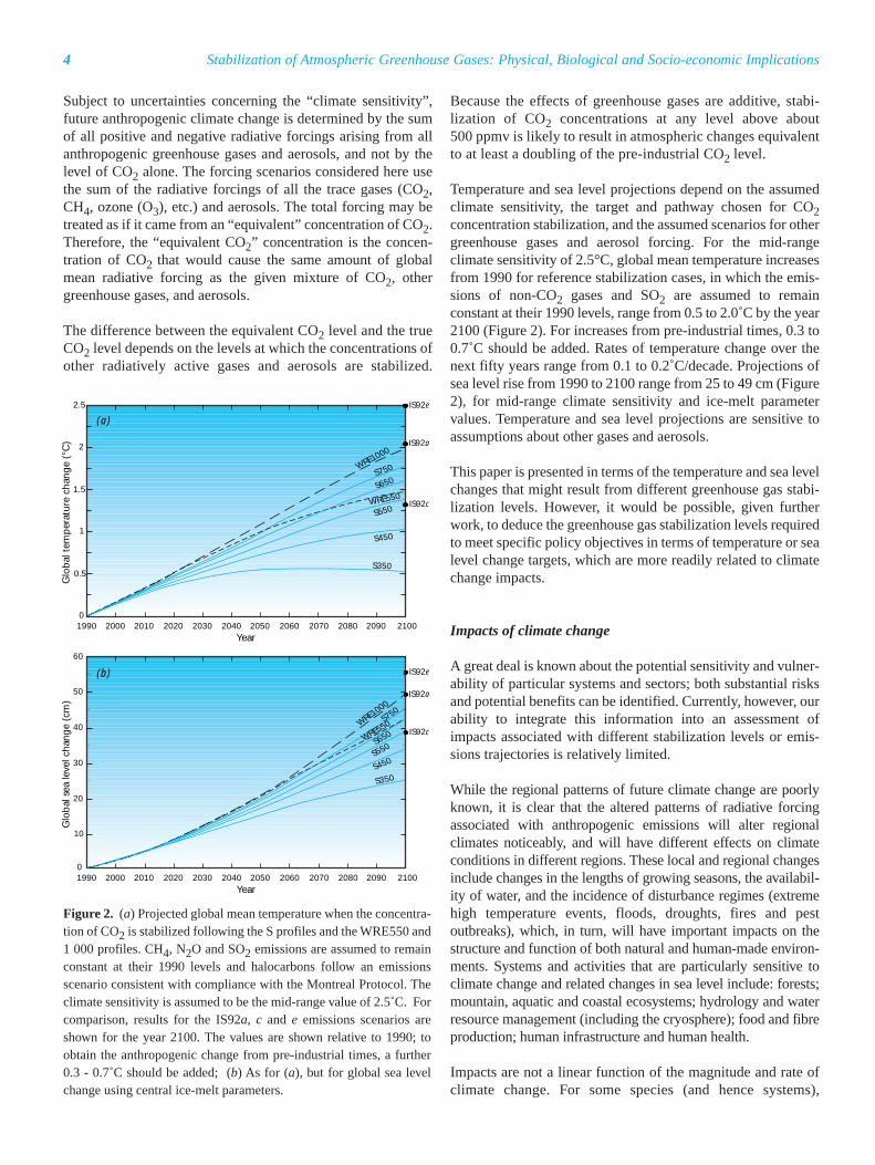
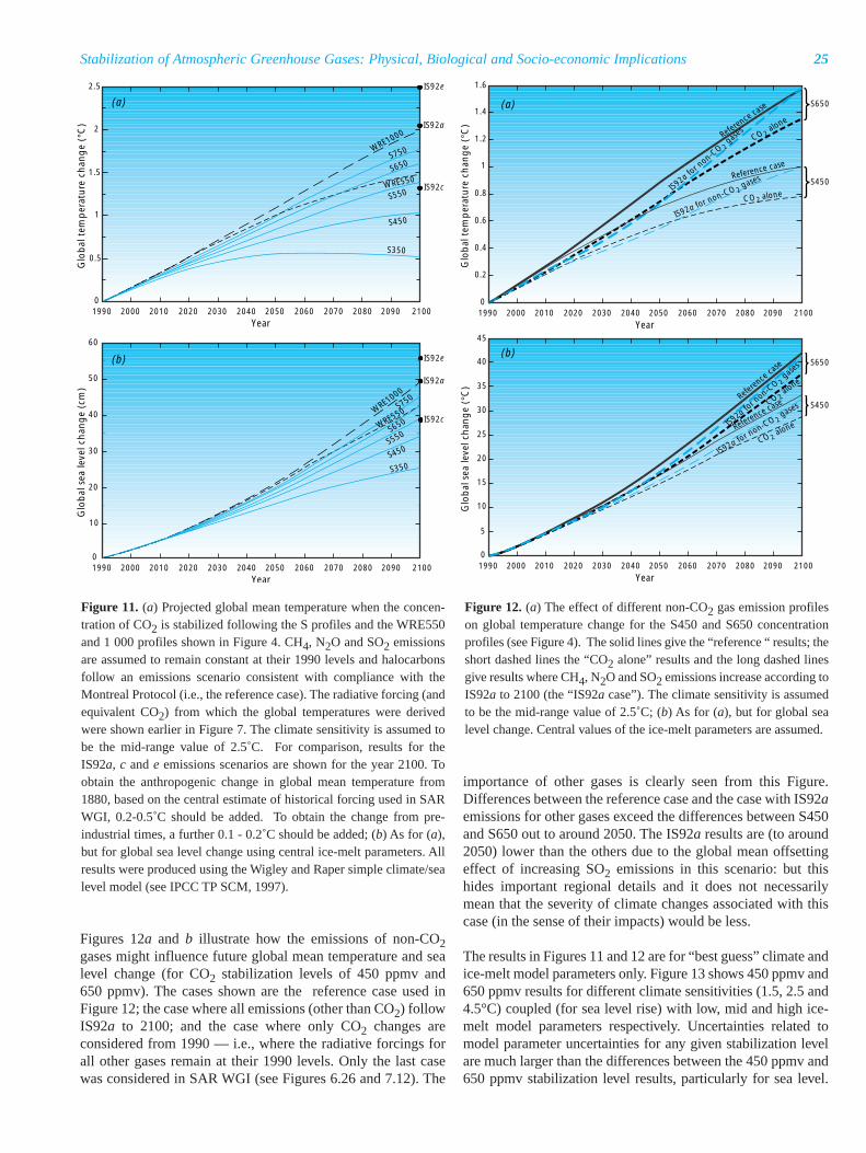
Temperature and sea level projections depend on the assumedclimate sensitivity, the target and pathway chosen for CO2concentration stabilization, and the assumed scenarios for othergreenhouse gases and aerosol forcing. For the mid-rangeclimate sensitivity of 2.5°C, global mean temperature increasesfrom 1990 for reference stabilization cases, in which the emis-sions of non-CO2 gases and SO2 are assumed to remainconstant at their 1990 levels, range from 0.5 to 2.0˚C by the year2100 (Figure 2). For increases from pre-industrial times, 0.3 to0.7˚C should be added. Rates of temperature change over thenext fifty years range from 0.1 to 0.2˚C/decade. Projections ofsea level rise from 1990 to 2100 range from 25 to 49 cm (Figure2), for mid-range climate sensitivity and ice-melt parametervalues. Temperature and sea level projections are sensitive toassumptions about other gases and aerosols.
This paper is presented in terms of the temperature and sea levelchanges that might result from different greenhouse gas stabi-lization levels. However, it would be possible, given furtherwork, to deduce the greenhouse gas stabilization levels requiredto meet specific policy objectives in terms of temperature or sealevel change targets, which are more readily related to climatechange impacts.
Impacts of climate change
A great deal is known about the potential sensitivity and vulner-ability of particular systems and sectors; both substantial risksand potential benefits can be identified. Currently, however, ourability to integrate this information into an assessment ofimpacts associated with different stabilization levels or emis-sions trajectories is relatively limited.
While the regional patterns of future climate change are poorlyknown, it is clear that the altered patterns of radiative forcingassociated with anthropogenic emissions will alter regionalclimates noticeably, and will have different effects on climateconditions in different regions. These local and regional changesinclude changes in the lengths of growing seasons, the availabil-ity of water, and the incidence of disturbance regimes (extremehigh temperature events, floods, droughts, fires and pestoutbreaks), which, in turn, will have important impacts on thestructure and function of both natural and human-made environ-ments. Systems and activities that are particularly sensitive toclimate change and related changes in sea level include: forests;mountain, aquatic and coastal ecosystems; hydrology and waterresource management (including the cryosphere); food and fibreproduction; human infrastructure and human health.
Impacts are not a linear function of the magnitude and rate ofclimate change. For some species (and hence systems),
Stabilization of Atmospheric Greenhouse Gases: Physical, Biological and Socio-economic Implications4
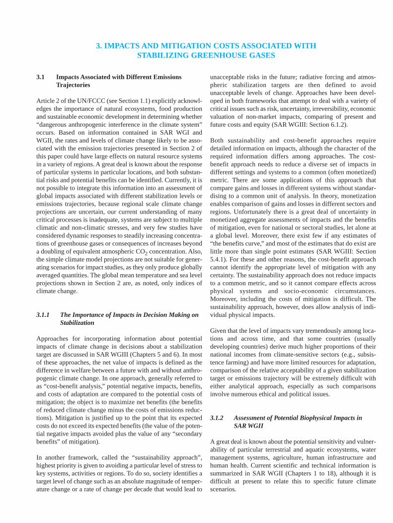
Figure 2. (a) Projected global mean temperature when the concentra-tion of CO2 is stabilized following the S profiles and the WRE550 and1 000 profiles. CH4, N2O and SO2 emissions are assumed to remainconstant at their 1990 levels and halocarbons follow an emissionsscenario consistent with compliance with the Montreal Protocol. Theclimate sensitivity is assumed to be the mid-range value of 2.5˚C. Forcomparison, results for the IS92a, c and e emissions scenarios areshown for the year 2100. The values are shown relative to 1990; toobtain the anthropogenic change from pre-industrial times, a further0.3 - 0.7˚C should be added; (b) As for (a), but for global sea levelchange using central ice-melt parameters.
thresholds of change in temperature, precipitation or otherfactors may exist, which, once exceeded, may lead to discon-tinuous changes in viability, structure or function. Theaggregation of impacts to produce a global assessment is notcurrently possible because of uncertainties regarding regionalclimate changes and regional responses, the difficulty ofvaluing impacts on natural systems and human health, andissues related to both interregional and intergenerational equity.
The ultimate concentration of greenhouse gases reached in theatmosphere, as well as the speed at which concentrationsincrease, is likely to influence impacts, because a slower rate ofclimate change will allow more time for systems to adapt.However, knowledge is not currently sufficient to identify clearthreshold rates and magnitudes of change.
Mitigation costs of stabilizing CO2 concentrations
Factors that affect CO2 mitigation costs include:
(a) Future emissions in the absence of policy intervention(“baselines”);
(b) The concentration target and route to stabilization, whichdetermine the carbon budget available for emissions;
(c) The behaviour of the natural carbon cycle, which influ-ences the emissions carbon budget available for any chosenconcentration target and pathway;
(d) The cost differential between fossil fuels and carbon-freealternatives and between different fossil fuels;
(e) Technological progress and the rate of adoption of tech-nologies that emit less carbon per unit of energy produced;
(f) Transitional costs associated with capital stock turnover,which increase if carried out prematurely;
(g) The degree of international cooperation, which determinesthe extent to which low cost mitigation options in differentparts of the world are implemented; and
(h) Assumptions about the discount rate used to compare costsat different points in time.
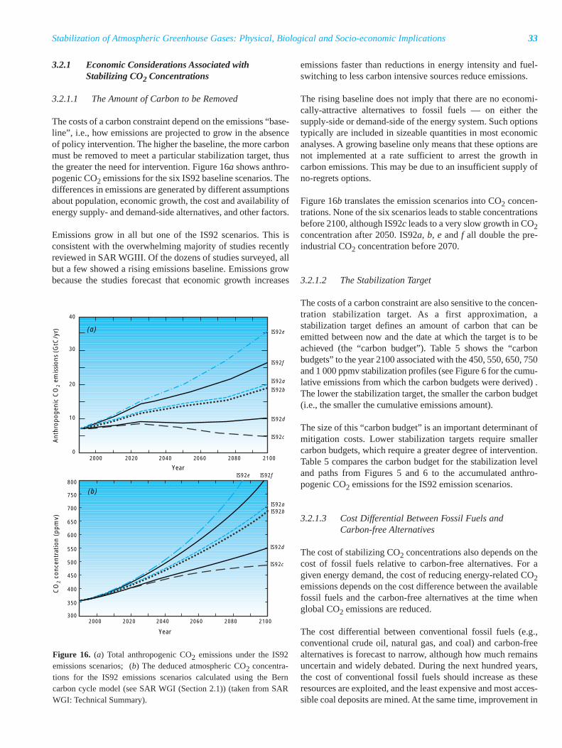
The costs of reducing emissions depend on the emissions“baseline”, i.e., how emissions are projected to grow in theabsence of policy intervention. The higher the baseline, themore carbon must be removed to meet a particular stabiliza-tion target, thus the greater the need for intervention. Thecosts of emissions reductions are also sensitive to theconcentration stabilization target. As a first approximation, astabilization target defines an amount of carbon that can beemitted between now and the date at which the target is to beachieved (the “carbon budget”). The size of the “carbon
budget” is an important determinant of mitigation costs.Lower stabilization targets require smaller carbon budgets,which require a greater degree of intervention.
The cost of stabilizing CO2 concentrations also depends on thecost of fossil fuels relative to carbon-free alternatives. The costof meeting a stabilization target generally increases with thecost difference between fossil fuels and carbon-free alterna-tives. A large cost differential implies that consumers mustincrease their expenditures on energy significantly to reduceemissions by replacing fossil fuels with carbon-free alterna-tives. The cost difference between unconventional fossil fuelsand carbon-free alternatives is likely to be smaller than thedifference between conventional oil and gas and carbon-freealternatives. If oil and gas still contribute significantly to theenergy mix at the time when global CO2 emissions must bereduced consistent with a given stabilization target, transitioncosts will be higher than if oil and gas compose a small part ofenergy use. While the cost premium for carbon-free alternativesis likely to be smaller for higher stabilization levels, we cannotpredict how this cost differential will change over time. Since,in addition, total energy demand is larger for higher stabiliza-tion levels, the net effect on the transition costs for differentstabilization levels is not clear.
A given concentration target may be achieved through morethan one emission pathway. Emissions in the near-term may bebalanced against emissions in the long-term. For a given stabi-lization level, there is a “budget” of allowable accumulatedcarbon emissions and the choice of pathway to stabilizationmay be viewed as a problem of how to best (i.e., with the great-est economic efficiency and least damaging impacts) allocatethis carbon budget over time. The differences in the emissionspath for the same stabilization level are important because costsdiffer among pathways. Higher early emissions decrease theoptions to adjust emissions later on.
Energy-related capital stock is typically long-lived and prema-ture retirement is apt to be costly. To avoid premature retirement,mitigation efforts can be spread more evenly over time andspace. The cost of any stabilization target can be reduced byfocusing on new investments and replacements at the end of theeconomic life of plant and equipment (i.e., at the point of capitalstock turnover), which is a continuous processes.
The cost of a stabilization path also depends on how technologyaffects the cost of abating emissions at a point in time and overtime. In general, the cost of an emission pathway increases withthe amount of emissions that must be abated at any point in time.The technological changes needed to lower the cost of abatingemissions will require a mix of measures. Greatly increasedgovernment research and development, removal of market barri-ers to technology development and dissemination, explicitmarket supports, tax incentives and appropriate emissionconstraints will probably act together to stimulate the technologyneeded to lower the costs of stabilizing atmospheric CO2concentration.
5Stabilization of Atmospheric Greenhouse Gases: Physical, Biological and Socio-economic Implications
With regard to mitigation costs, a positive discount rate lowersthe present value of the costs incurred. This is because it placesa lower weight on investments made in the future. Indeed, thefurther in the future an economic burden (here, emission reduc-tions) lies, the lower the present value of costs. In a widercontext, discounting reduces the weight placed on future envi-ronmental impacts relative to the benefits of current energy use.Its use makes serious challenges, such as rapid switching ofenergy systems in the future, seem easy in terms of presentdollars and may affect consideration of intergenerational equity.
Integrating information on impacts and mitigation costs
This report provides a framework for integrating information onthe costs, benefits and impacts of climate change.Concentration stabilization profiles that follow “business-as-usual” emissions for periods of a few to several decades shouldnot be construed as a suggestion that no action is required forthose periods. In fact, studies suggest that even in those cases ofbusiness-as-usual emissions for some period of time, actionsmust be taken during that time to cause emissions to declinesubsequently. The strategies for developing portfolios of actionsleading to immediate or eventual reductions below business-as-usual are discussed below.
Numerous policy measures are available to facilitate adaptationto climate change, to reduce emissions of greenhouse gases, andto create technologies that will reduce emissions in the future.If expressed in terms of CO2 equivalent or total radiativeforcing, a given stabilization level can be met through variouscombinations of reductions in the emissions of different gasesand by enhancing sinks of greenhouse gases. Governmentsmust decide both the amount of resources to devote to this issueand the mix of measures they believe will be most effective.IPCC WGIII (1996)2 states that significant “no-regrets”3
measures are available. Because no-regrets policies currentlyare beneficial, the issues facing governments are how to imple-ment the full range of no-regrets measures and whether, and ifso, when and how far to proceed beyond purely no-regretsoptions. The risk of aggregate net impacts due to climatechange, consideration of risk aversion, and the application ofthe precautionary principle provide rationales for action beyondno-regrets.
Stabilization of Atmospheric Greenhouse Gases: Physical, Biological and Socio-economic Implications6
2 Hereafter referred to as SAR WGIII.3 “No regrets” measures are those whose benefits, such as reduced
energy costs and reduced emissions of local/regional pollutants,equal or exceed their cost to society, excluding the benefits ofclimate change mitigation.
1.1 Aims
Based on material in the IPCC Second Assessment Report(IPCC WGI, WGII and WGIII, 19964), this Technical Paperexpands and clarifies the scientific and technical issues relevantto interpreting the objective of the United Nations FrameworkConvention on Climate Change (UN/FCCC) as stated in Article 2 (United Nations, 1992):
“The ultimate objective of this Convention and any related legalinstruments that the Conference of the Parties may adopt is toachieve, in accordance with the relevant provisions of theConvention, stabilization of greenhouse gas concentrations inthe atmosphere at a level that would prevent dangerous anthro-pogenic interference with the climate system. Such a levelshould be achieved within a time frame sufficient to allowecosystems to adapt naturally to climate change, to ensure thatfood production is not threatened and to enable economic devel-opment to proceed in a sustainable manner.”
Article 2 requires stabilization of greenhouse gas concentra-tions. Here we emphasize CO2, but we also consider severalother gases to illustrate the uncertainties associated with a moregeneral multi-gas stabilization objective and to highlight whatcan be said with some confidence.
The clear historical relationship between CO2 emissions andchanging atmospheric concentrations, as well as our consider-able knowledge of the carbon cycle, implies that continuedfossil fuel, cement production, and land-use related emissionsof CO2 at historical, present, or higher rates in the future willincrease atmospheric concentrations of this greenhouse gas.Understanding how CO2 concentrations change in the futurerequires quantification of the relationship between CO2 emis-sions and atmospheric concentration using models of the carboncycle.
This paper draws on information presented in SAR WGI, WGIIand WGIII. We first review the results of a range of standard-ized calculations (presented in the 1994 IPCC Report5 and SARWGI) used to analyse the relationships between emissions andconcentrations for several levels of atmospheric CO2 stabiliza-tion, including two pathways to reach each level. We thenconsider the effects of other greenhouse gases and sulphateaerosol (from SO2 emissions), and estimate the temperature andsea level changes associated with the various stabilization levelsstudied. Finally, we review briefly the potential positive andnegative impacts associated with the projected temperature andsea level changes, and discuss the mitigation costs associatedwith stabilizing greenhouse gases.
The temperature change and sea level rise projections are calcu-lated using the simplified models used in SAR WGI, modelsthat have been calibrated against more complex models. Thesemore complex models are not used for the analyses presentedhere because they are too expensive and time consuming to runfor the large number of cases studied here, and because theirglobal mean results may be adequately represented usingsimpler models (see IPCC Technical Paper: An Introduction toSimple Climate Models used in the IPCC Second AssessmentReport (IPCC TP SCM, 1997)).
A range of alternative concentration profiles were employed inSAR WGI to assess the potential climatic consequences of: (a)stabilizing CO2 concentrations via a range of pathways; (b) plau-sible future emissions scenarios for trace gases other than CO2;and (c) several levels of future SO2 emissions (leading to differ-ent levels of aerosol). In the context of Article 2, it is important toinvestigate a range of emissions profiles of greenhouse gases thatmight stabilize atmospheric concentrations so that differentpossibilities and impacts can be considered. In addition, evaluat-ing several profiles avoids making any judgement about the ratesor magnitudes of climate change that would qualify as “danger-ous interference”. Because an understanding of the constraints onthe stabilization of greenhouse gases is fundamental to policyformulation with regard to the goals of the UN/FCCC and itsimplementation, this Technical Paper provides both a tutorial andan expanded evaluation of the stabilization calculations presentedin IPCC94 and SAR WGI and WGIII.
The Technical Paper will specifically:
(a) Present a tutorial on stabilization of greenhouse gases, theestimation of radiative forcing, and the concept of “equiv-alent CO2” (the concentration of CO2 that leads to globalmean radiative forcing consistent with projected increasesin all gases when a suite of gases is being considered);
(b) Present a basic set of CO2 stabilization profiles leading, viatwo types of pathway, to stabilization between 350 and750 ppmv, with a single profile stabilizing at 1 000 ppmv;
(c) Present the deduced emissions for the aforementionedconcentration stabilization profiles;
(d) Consider stabilization of radiative forcing agents other thanCO2;
(e) Compute (using a simplified climate model) global meantemperature and sea level changes for the CO2 profilesusing a range of emissions assumptions for CH4, N2O andSO2, and different values of the climate sensitivity and ice-melt model parameter values in order to characteriseuncertainties (see IPCC TP SCM, 1997 for a discussion ofsimple climate models);
1. INTRODUCTION
4 Hereafter referred to as SAR WGI, SAR WGII and SAR WGIII.5 IPCC, 1995, hereafter referred to as IPCC94.
(f) Discuss the potential environmental consequences of thederived changes in temperature and sea level;
(g) Discuss the factors that influence mitigation costs; and
(h) Review the methodology for integrating climate and sealevel change effects and mitigation costs to produce a morecomplete view of the consequences of changing atmos-pheric composition.
1.2 Key Points
1.2.1 Some Fundamentals Regarding Greenhouse Gasesand Tropospheric Aerosols (see SAR WGI for moredetails)
Of the greenhouse gases, this paper focuses on CO2 because ithas had, and is projected to have, the largest effect on radiativeforcing (in 1990, 1.56 W m-2 for CO2 versus 0.47 W m-2 forCH4, 0.14 W m-2 for N2O and 0.27 W m-2 for the halocarbons).For a discussion of the utility of radiative forcing in climatechange studies see IPCC94 (Chapter 4) and IPCC TP SCM(1997). This paper also considers the effects that arise when aseries of assumptions are made about potential future emissionsof other greenhouse gases and SO2, a primary aerosol precursor(aerosols may act to cool the planet).
Tropospheric aerosols (microscopic airborne particles) result-ing from combustion of fossil fuels, biomass burning, and otheranthropogenic sources have led to a highly uncertain estimate ofdirect forcing of -0.5 W m-2 (range: -0.25 to -1.0 W m-2) overthe past century as a global average. There is possibly also anegative indirect forcing – via modifications of clouds – thatremains very difficult to quantify (SAR WGI: Chapter 2).Because aerosols have short lifetimes in the atmosphere, theirdistribution and hence immediate radiative effects are veryregional in character. Locally, the aerosol forcing can be largeenough to more than offset the positive forcing due to green-house gases. However, although the negative forcing is focusedin particular regions and subcontinental areas, it has continentalto hemispheric scale effects on climate because of couplingsthrough atmospheric circulation.
1.2.2 Stabilization of CO2 Concentrations (see SAR WGIfor more details)
Among the range of stabilization cases studied, accumulatedanthropogenic emissions from 1991 to 2100 fall between 630and 1410 GtC, for stabilization levels between 450 and 1000ppmv. For comparison, the corresponding accumulated emis-sions for the IPCC IS92 emissions scenarios range from 770 to2190 GtC.
For each stabilization level from 350 to 750 ppmv, two path-ways are considered: the “S” pathways, that depart immediately
from IS92a, and the “WRE” pathways that follow IS92ainitially. A single pathway that stabilizes at 1 000 ppmv is alsoconsidered. The WRE pathways imply higher emissions in theshort-term, but an earlier and more rapid change from increas-ing to decreasing emissions, and lower emissions later.
Ecosystem and oceanic feedbacks may reduce terrestrial andoceanic carbon storage to levels somewhat below thoseassumed in the simplified global carbon cycle models used hereand in the Second Assessment Report. Uncertainties resultingfrom the omission of potentially critical oceanic and biosphericprocesses during transient climate change could have a signifi-cant effect on the conclusions regarding emissions associatedwith stabilization.
1.2.3 Taking the Climatic Effects of Other GreenhouseGases and Aerosols into Account: the Concept ofEquivalent CO2
Subject to uncertainties concerning the climate sensitivity (seebelow), future anthropogenic climate change is determined bythe sum of all positive and negative forcings arising from allanthropogenic greenhouse gases and aerosols, not by the levelof CO2 alone. The forcing scenarios used in many of the modelruns are the sum of the radiative forcings of all the trace gases(CO2, CH4, O3, etc.) and aerosols. The total forcing may betreated as if it came from an “equivalent” concentration of CO2.Therefore, the “equivalent CO2” concentration is the concen-tration of CO2 that would cause the same amount of globalmean radiative forcing as the given mixture of CO2, othergreenhouse gases, and aerosols.
The difference between the equivalent CO2 level and the trueCO2 level depends on the levels at which the concentrations ofother radiatively active gases and aerosols are stabilized. Thestabilization levels chosen for CH4, N2O and SO2 can signifi-cantly affect equivalent CO2. If the emissions of these gaseswere held constant at today’s levels, equivalent CO2 wouldstabilize at approximately 26 ppmv (S350) to 74 ppmv(WRE1000) ppmv above the level for CO2 alone. Because theeffects of greenhouse gases are additive, stabilization of CO2concentrations at any level above about 500 ppmv is likely toresult in atmospheric changes equivalent to at least a doublingof the pre-industrial CO2 level.
1.2.4 The Global Temperature and Sea LevelImplications of Stabilizing Greenhouse Gases
This report considers two simple indices of climate change,global mean temperature and sea level rise. The change inglobal mean temperature is the main factor determining the risein sea level; it is also a useful proxy for overall climate change.It is important to realize, however, that climate change will notoccur uniformly over the globe; the changes in temperature andin other climate variables such as precipitation, cloudiness, and
Stabilization of Atmospheric Greenhouse Gases: Physical, Biological and Socio-economic Implications8
the frequency of extreme events, will vary greatly amongregions. In order to evaluate the consequences of climatechange, one must consider the spatial variability of all factors:climate forcing, climate response, and the vulnerability ofregional human and natural resource systems. However, consid-eration of regional details is outside the scope of this paper.
The spatial patterns of some radiative forcing agents, especiallyaerosols, are very heterogeneous and so add further to thespatial variability of climate change. In this paper, aerosolforcing is presented in terms of global averages so that animpression can be gained of its likely overall magnitude, itseffect on global average temperature, and its effect on sea levelrise. The effect of aerosol forcing on the detail of climatechange, however, is likely to be quite different from the effect ofa forcing of similar magnitude, in terms of global average, dueto greenhouse gases. In terms of regional climate change andimpacts, therefore, the negative forcing or cooling from aerosolforcing must not be considered as a simple offset to that fromgreenhouse gases.
Temperature and sea level projections depend on the assumedclimate sensitivity, the target and pathway chosen for CO2concentration stabilization, and the assumed scenarios for othergreenhouse gases and aerosol forcing. The relative importanceof these factors depends on the time interval over which they arecompared. Out to the year 2050, CO2 concentration pathwaydifferences for any single stabilization target are as important asthe choice of target; but on longer time-scales the choice oftarget is (necessarily) more important. Outweighing all of thesefactors, however, is the climate sensitivity, uncertainties inwhich dominate the uncertainties in all projections.
1.2.5 Impacts
A great deal is known about the potential sensitivity and vulner-ability of particular systems and sectors, and both substantialrisks and potential benefits can be identified. Currentlyhowever, our ability to integrate this information into an assess-ment of impacts associated with different stabilization levels oremissions trajectories is relatively limited.
While the regional patterns of future climate change are poorlyknown, it is clear that the altered patterns of radiative forcingassociated with anthropogenic emissions will alter regionalclimates noticeably, and will have different effects on climateconditions in different regions. These local and regionalchanges will necessarily include changes in the lengths ofgrowing seasons, the availability of water, and the incidence ofdisturbance regimes (extreme high temperature events, floods,droughts, fires, and pest outbreaks), which, in turn, will haveimportant impacts on the structure and function of both naturaland human-made environments. Systems and activities that areparticularly sensitive to climate change and related changes insea level include: forests; mountain, aquatic and coastal ecosys-tems; hydrology and water resource management (including the
cryosphere); food and fibre production; human infrastructureand human health. Most existing impacts studies are analyses ofwhat may result from the equilibrium climate changes associ-ated with a doubled equivalent CO2 level; few studies haveconsidered responses over time to more realistic conditionsinvolving increasing concentrations of greenhouse gases.
Impacts are not a linear function of the magnitude and rate ofclimate change. For some species (and hence systems), thresh-olds of change in temperature, precipitation, or other factorsmay exist, which, once exceeded, may lead to discontinuouschanges in viability, structure, or function.
Aggregation of impacts to produce a global assessment is notcurrently possible because of our lack of knowledge of regionalclimate changes and regional responses, because of the diffi-culty of valuing impacts on natural systems and human health,and because of issues related to both interregional and inter-generational equity.
The ultimate concentration of greenhouse gases reached in theatmosphere, as well as the speed at which concentrationsincrease, is likely to influence impacts, because a slower rate ofclimate change will allow more time for systems to adapt.However, knowledge is not currently sufficient to identify clearthreshold rates and magnitudes of change.
1.2.6 Mitigation Costs of Stabilizing CO2 Concentrations
Factors that affect CO2 mitigation costs include:
(a) Future emissions in the absence of policy intervention(“baselines”);
(b) The concentration target and route to stabilization, whichdetermine the carbon budget available for emissions;
(c) The behaviour of the natural carbon cycle, which influ-ences the emissions carbon budget available for any chosenconcentration target and pathway;
(d) The cost differential between fossil fuels and carbon-freealternatives and between different fossil fuels;
(e) Technological progress and the rate of adoption of tech-nologies that emit less carbon per unit of energy produced;
(f) Transitional costs associated with capital stock turnover,which increase if carried out prematurely;
(g) The degree of international cooperation, which determinesthe extent to which low cost mitigation options in differentparts of the world are implemented; and
(h) Assumptions about the discount rate used to compare costsat different points in time.
9Stabilization of Atmospheric Greenhouse Gases: Physical, Biological and Socio-economic Implications
1.2.7 Integrating Information on Impacts and MitigationCosts
This reports provides a framework for integrating information onthe costs, benefits and impacts of climate change. The pointsbelow must be prefaced with the critical observation that concen-tration stabilization profiles that follow “business-as-usual”emissions for periods of a few to several decades should not beconstrued as a suggestion that no action is required for thoseperiods. In fact, studies suggest that even in those cases of busi-ness-as-usual emissions for some period of time, actions must betaken during that time to cause emissions to decline subsequently.The strategies for developing portfolios of actions leading toimmediate or eventual reductions below business-as-usual arediscussed below.
This paper is designed to demonstrate how information can beassembled on the costs, impacts and benefits of stabilizing atmos-pheric greenhouse gases. This analysis, which supports manydecision making formats, has two “branches”. The first branch,“impacts”, assembles information beginning with assumedconcentration changes, and then evaluates potential climatechange, and its consequences. The second branch, “mitigation”,assembles information on emissions and mitigation costs associ-ated with achieving a range of stabilization pathways and levels.The two branches must be combined to produce an integratedassessment of climate change and stabilization (Figure 3).
If expressed in terms of CO2 equivalent or total radiative forcing,a given stabilization level can be met through various combina-tions of reductions in the emissions of different gases and byenhancing sinks of greenhouse gases. Considering all suchoptions, and selecting the least expensive ones while takingaccount of different sources and sinks, should lower the costs ofmitigation. Approaching an optimum mix requires informationabout the concentration and climate implications of differentemissions strategies, the mitigation costs and other characteristicsof the different options, and decisions about the appropriate time-scales and indices of impacts (climate and non-climate) to be usedin comparing the different gases. Because of high uncertainty, asimproved information becomes available, these mixes of optionsmust be re-evaluated and modified in an evolving process.
In order to implement a portfolio of actions to address climatechange, governments must decide both the amount of resourcesto devote to this issue and the mix of measures they believe willbe most effective. Because no-regrets policies are currently bene-ficial, the issues facing governments are how to implement thefull range of no-regrets measures and whether, and if so, whenand how far to proceed beyond purely no-regrets options. Therisk of aggregate net impacts due to climate change, considera-tion of risk aversion, and the application of the precautionaryprinciple provide rationales for action beyond no-regrets (SARWGIII).
Numerous policy measures are available to facilitate adaptationto climate change, to reduce emissions of greenhouse gases, and
to create technologies that will reduce emissions in the future.These include immediate reductions in emissions to slowclimate change; research and development on new supply andconservation technologies to reduce future abatement costs;continued research to reduce critical scientific uncertainties;and investments in actions to help human and natural systemsadapt to climate change through mitigation of negative impactsand through advantages resulting from increasing CO2 (e.g.,increased water or nutrient use efficiency of some crops withelevated CO2). The issue is not one of “either-or” but one offinding the right mix (i.e., portfolio) of options, taken togetherand sequentially. The mix at any point in time will vary anddepend upon the concentration objective, which may itself beadjusted with advances in the scientific and economic knowl-edge base. The appropriate portfolio also varies amongcountries and depends upon energy markets, economic consid-erations, political structure, and societal receptiveness.
1.3 A “Road map” to this Report
1.3.1 Report Strategy
The organization of this report is illustrated in Figure 3. Thisorganization is designed to assemble important informationrelevant to a wide variety of policy makers concerned withimplementing the goal of the UN/FCCC. Information falls intotwo general categories needed to understand the costs and bene-fits associated with atmospheric stabilization. The first category(or “branch”) assembles information about climate change, andits consequences, whereas the second category assembles infor-mation about emissions and mitigation costs. This approachorganizes information from SAR WGI, WGII and WGIII rele-vant to the issue of greenhouse gas stabilization for use in amore integrated analysis.
The strategy chosen flows forward from SAR WGI, whichconsiders a series of concentration profiles as a basis for deduc-ing anthropogenic emissions consistent with the underlying
Stabilization of Atmospheric Greenhouse Gases: Physical, Biological and Socio-economic Implications10
Integratedassessment
Mitigationanalysis
Concentrations
Emissions
Climatechange
Radiativeforcing
Impacts
Mitigation costs
Impacts
Figure 3. An overview of the structure and logic of this TechnicalPaper.
physics and biology of oceanic and terrestrial ecosystems, albeitsimplified (see Section 2.2.1.3 on uncertainties). Beginningwith concentration profiles, we calculate, using simplifiedclimate models from SAR WGI (Section 6.3), the global meantemperature and sea level consequences of these CO2 concen-tration profiles (covered in Section 2.3). We also carry outsensitivity analyses showing the effects of other gases andaerosols on these central CO2 analyses. These global meantemperature and sea level changes provide a context for consid-ering the consequences for natural resources, infrastructure,human health, and other sectors affected by the climate(covered in Section 3.1). This completes the “impacts branch”of the analysis (see Figure 3). Note that this analysis providesonly a simplified global mean view of consequences. For amore appropriately detailed view, regional climate changes andsystem vulnerabilities must be considered (see SAR WGI:Chapter 6 and SAR WGII for discussions of regional climatechange and vulnerabilities).
The “mitigation costs branch” of this analysis also begins withconcentration profiles (see Figure 3). The concentration profilesare then used together with carbon cycle models (see SARWGI: Section 2.1 and IPCC94: Section 1.5) to compute anthro-pogenic emissions (covered in Section 2.2.1). These deducedemissions can be used in economic models to estimate the“mitigation” costs of following the stabilization profile ratherthan a business-as-usual trajectory (covered in Section 3.2),given the appropriate assumptions. Mitigation costs can becomputed for a wide range of stabilization profiles and withmultiple economic models to provide a sense of the range ofpossible mitigation costs as a function of an eventual stabiliza-tion target and pathway. Note that all of these analyses considerthe economic costs for mitigation associated with particularspecified concentration profiles. They are thus not “optimal”trajectories nor do they represent policy recommendations.Rather, they are illustrative of the links from concentrations toemissions and thence to mitigation costs.
The two branches come together, conceptually, in the end in thesection on integrating information on impacts and mitigationcosts (Section 3.3). Neither branch provides a complete basis for
decision making. This general type of problem supports a widerange of decision-making frameworks, which may integrate thisinformation in a variety of ways (see SAR WGIII: Chapter 4).
1.3.2 Decision-making Frameworks
Although it is important to assemble information about thecosts and benefits associated with atmospheric stabilization,assemblage is not the same as recommending a simple cost-benefit analysis. The cost-benefit paradigm is the most familiardecision related application of the economics of balancing costsand benefits, but it is not the only approach available. Othertechniques include cost effectiveness analysis, multi-criteriaanalysis, and decision analysis (SAR WGIII, p.151). Decision-making frameworks must consider uncertainty in projectedconcentration changes, in consequent climate effects, and inconsequences for human and natural systems. A wide range ofparadigms for dealing with this uncertainty likewise exist, andare summarized in SAR WGIII.
The analysis of biophysical and economic uncertaintiespresented in this report is only a brief summary of issues. Whilea more detailed discussion can be found in SAR WGI, WGII,and WGIII, the full dimensions of uncertainty in the analysislinking concentrations to, ultimately, costs and consequences,remains an active area of investigation. Regardless of themethod eventually employed in the decision-making process,information about the costs and benefits of emissions mitigationcan be used to improve the quality of policy decisions.
The present document makes no attempt to judge the practicalissues of implementing emissions mitigation strategies, nordoes it consider the fairness and equity concerns that surroundsuch deliberations. The global perspective employed here is formethodological and pedagogical convenience: it is not meant toimply that regional issues are less important — clearly, climatepolicy must be made within the context of a wide array ofnational and international policy considerations. Such mattersadd to the rich complexity of issues with which policy makersmust grapple.
11Stabilization of Atmospheric Greenhouse Gases: Physical, Biological and Socio-economic Implications
2.1 General Principles of Stabilization: Stabilization ofCarbon Dioxide and Other Gases
There has been confusion about the scientific aspects of stabi-lizing the atmospheric CO2 concentration vis-à-vis thestabilization of the concentrations of other gases, particularlywith regard to the concept of “lifetime”. The processes thatcontrol the lifetimes of the key gases are reviewed in detail inSAR WGI (Chapter 2) and IPCC94, which provides vital back-ground material for this brief review.
Most carbon reservoirs exchange CO2 with the atmosphere:they both absorb (oceans) or assimilate (ecosystems), andrelease (oceans) or respire (ecosystems) CO2. The criticalpoint here is that anthropogenic carbon emitted into theatmosphere is not destroyed but adds to and is redistributedamong the carbon reservoirs. These reservoirs exchangecarbon between themselves on a wide range of time-scalesdetermined by their respective turnover times. Turnover timesrange from years to decades (carbon turnover in living plants)to millennia (carbon turnover in the deep sea and in long-lived soil pools). These time-scales are generally much longerthan the average time a particular CO2 molecule spends in theatmosphere, which is only about four years. The large rangeof turnover times has another remarkable consequence: therelaxation of a perturbed atmospheric CO2 concentrationtowards a new equilibrium cannot be described by a singletime constant. Thus, attempts to characterize the removal ofanthropogenic CO2 from the atmosphere by a single timeconstant (e.g., 100 years) must be interpreted in a qualitativesense only. Quantitative evaluations based on a single life-time are erroneous.
In contrast to CO2, aerosols and non-CO2 greenhouse gasessuch as the halocarbons, methane and N2O are destroyed (e.g.,by oxidation, photochemical decomposition, or, for aerosols, bydeposition on the ground). The time such a molecule (or parti-cle) spends on average in the atmosphere (i.e., its turnover time)is equal or roughly similar to the adjustment time.
Methane is emitted to the atmosphere from a range of sources(see SAR WGI) and is destroyed mainly through oxidation bythe hydroxyl radical (OH) in the atmosphere and by soil micro-organisms. The adjustment time of a perturbation inatmospheric methane is controlled by its oxidation (to CO2 andwater vapour) rather than by exchange with other reservoirs,which could subsequently re-release methane back to theatmosphere. Methane’s lifetime is complicated by feedbacksbetween methane and OH, such that increasing the methaneconcentration changes the methane removal rate by -0.17 to+0.35 per cent per 1 per cent increase in methane (SAR WGI:Section 2.2.3.1). Many other feedback processes in the CH4—CO—O3—OH—NOx—UV system also influence the lifetime
of methane. Methane can be stabilized on the time-scale of itsatmospheric lifetime: decades or less.
Nitrous oxide has a long lifetime, 100 to 150 years. N2O isremoved from the troposphere (where it acts as a greenhousegas) by exchange with the stratosphere where it is slowlydestroyed by photochemical decomposition. Like methane, itslifetime is controlled by its destruction rate, and, like methane,it is destroyed rather than exchanged with other reservoirs ofN2O. Stabilization of the N2O concentration requires reductionof sources, and such reductions would need to extend overlengthy periods to influence concentrations because of the~120-year lifetime of this gas. On the other hand, atmosphericaerosol concentration adjusts within days to weeks to a changein emissions of aerosols and aerosol precursor gases.
2.2 Description of Concentration Profiles, Other TraceGas Scenarios and Computation of Equivalent CO2
2.2.1 Emission Consequences of Stabilization
2.2.1.1 Concentration Profiles Leading to Stabilization
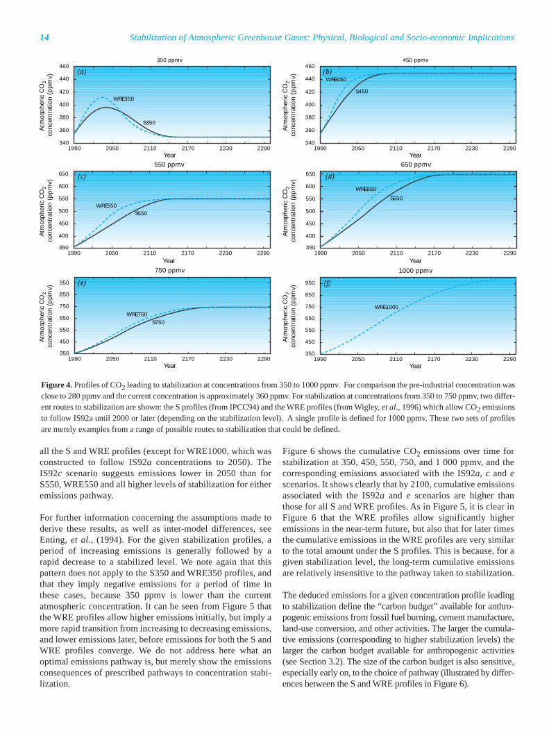
In this Technical Paper, we evaluate the 11 illustrative CO2concentration profiles (stabilizing at 350 to 1 000 ppmv,referred to as the “S” and “WRE” profiles) as discussed in SARWGI. These profiles prescribe paths of concentration with time,leading gradually to stabilization at the prescribed level (Figure 4). The WRE profiles prescribe larger increases in CO2concentration earlier in time when compared with the Sprofiles, but lead to the same stabilized levels (Wigley, et al.,1996). The concentration profiles can also be used as input tocompute a range of allowed emissions over time. Deducedemissions, in turn, can be used as inputs to economic models tocompute the mitigation costs associated with reducing emis-sions to follow a specified concentration profile. It should benoted that this approach does not allow calculation of, or implyanything about, optimal paths of emissions.
2.2.1.2 Emissions Implications of Stabilization of CO2Concentrations
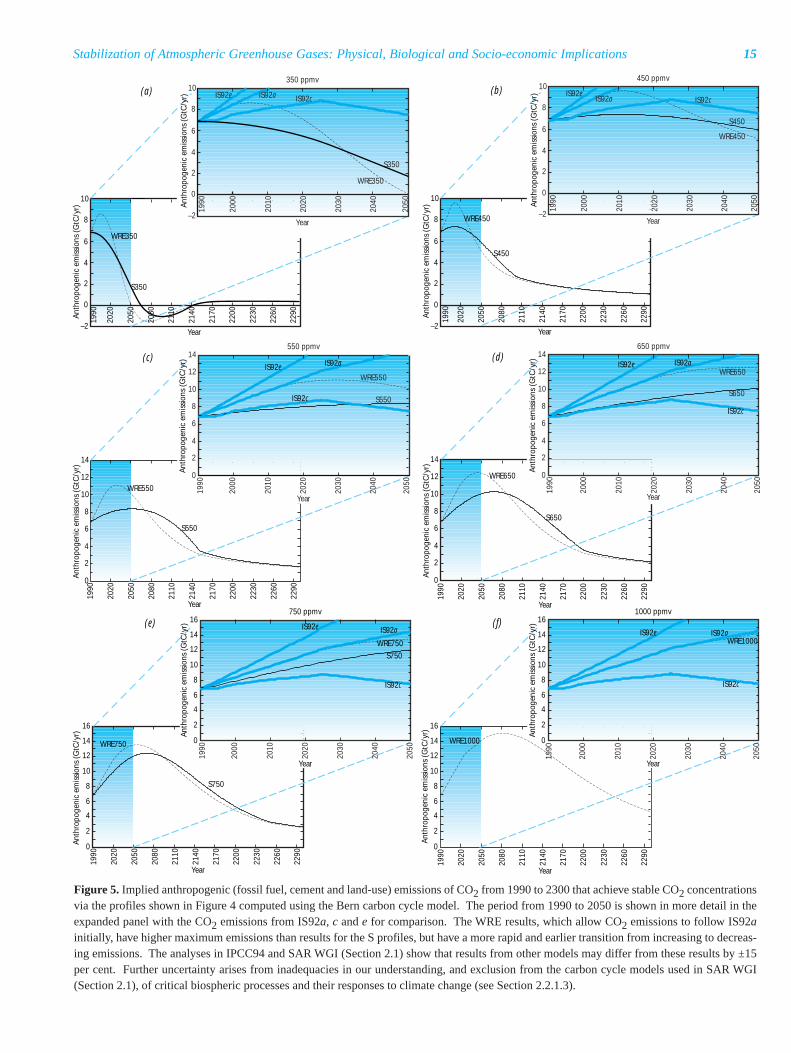
In this analysis, we again consider the S350–750 profiles andthe WRE350–1000 profiles described in IPCC94 (Chapter 1)and SAR WGI (Section 2.1), but more completely than waspossible in either of those documents. First, we presentgraphs showing CO2 concentrations versus time (Figure 4)and the corresponding emissions versus time for all 11profiles together with, for comparison, the IS92a, c, and escenarios (Figure 5). Note that CO2 emissions for the IS92aand e scenarios are higher in year 2050 than are emissions for
2. GEOPHYSICAL IMPLICATIONS ASSOCIATED WITH GREENHOUSE GASSTABILIZATION
all the S and WRE profiles (except for WRE1000, which wasconstructed to follow IS92a concentrations to 2050). TheIS92c scenario suggests emissions lower in 2050 than forS550, WRE550 and all higher levels of stabilization for eitheremissions pathway.
For further information concerning the assumptions made toderive these results, as well as inter-model differences, seeEnting, et al., (1994). For the given stabilization profiles, aperiod of increasing emissions is generally followed by arapid decrease to a stabilized level. We note again that thispattern does not apply to the S350 and WRE350 profiles, andthat they imply negative emissions for a period of time inthese cases, because 350 ppmv is lower than the currentatmospheric concentration. It can be seen from Figure 5 thatthe WRE profiles allow higher emissions initially, but imply amore rapid transition from increasing to decreasing emissions,and lower emissions later, before emissions for both the S andWRE profiles converge. We do not address here what anoptimal emissions pathway is, but merely show the emissionsconsequences of prescribed pathways to concentration stabi-lization.
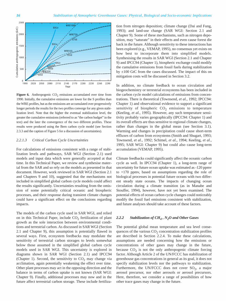
Figure 6 shows the cumulative CO2 emissions over time forstabilization at 350, 450, 550, 750, and 1 000 ppmv, and thecorresponding emissions associated with the IS92a, c and escenarios. It shows clearly that by 2100, cumulative emissionsassociated with the IS92a and e scenarios are higher thanthose for all S and WRE profiles. As in Figure 5, it is clear inFigure 6 that the WRE profiles allow significantly higheremissions in the near-term future, but also that for later timesthe cumulative emissions in the WRE profiles are very similarto the total amount under the S profiles. This is because, for agiven stabilization level, the long-term cumulative emissionsare relatively insensitive to the pathway taken to stabilization.
The deduced emissions for a given concentration profile leadingto stabilization define the “carbon budget” available for anthro-pogenic emissions from fossil fuel burning, cement manufacture,land-use conversion, and other activities. The larger the cumula-tive emissions (corresponding to higher stabilization levels) thelarger the carbon budget available for anthropogenic activities(see Section 3.2). The size of the carbon budget is also sensitive,especially early on, to the choice of pathway (illustrated by differ-ences between the S and WRE profiles in Figure 6).
Stabilization of Atmospheric Greenhouse Gases: Physical, Biological and Socio-economic Implications14A
tmos
pher
ic C
O2
con
cent
ratio
n (p
pmv)
Atm
osph
eric
CO
2 c
once
ntra
tion
(ppm
v)
Atm
osph
eric
CO
2 c
once
ntra
tion
(ppm
v)
Atm
osph
eric
CO
2 c
once
ntra
tion
(ppm
v)
Atm
osph
eric
CO
2 c
once
ntra
tion
(ppm
v)
Atm
osph
eric
CO
2 c
once
ntra
tion
(ppm
v)
460
S350
WRE350
440
420
400
380
360
3401990 2050 2110 2170 2230 2290
Year
350 ppmv460
S450
WRE450440
420
400
380
360
3401990 2050 2110 2170 2230 2290
Year
450 ppmv
S550WRE550
650
600
550
500
450
400
350
650
600
550
500
450
400
3501990 2050 2110 2170 2230 2290
Year
550 ppmv
S650
WRE650
1990 2050 2110 2170 2230 2290Year
650 ppmv
S750WRE750
950
850
750
650
550
450
3501990 2050 2110 2170 2230 2290
Year
750 ppmv
WRE1000
950
850
750
650
550
450
3501990 2050 2110 2170 2230 2290
Year
1000 ppmv
(a) (b)
(c) (d)
(e) (f)
Figure 4. Profiles of CO2 leading to stabilization at concentrations from 350 to 1000 ppmv. For comparison the pre-industrial concentration wasclose to 280 ppmv and the current concentration is approximately 360 ppmv. For stabilization at concentrations from 350 to 750 ppmv, two differ-ent routes to stabilization are shown: the S profiles (from IPCC94) and the WRE profiles (from Wigley, et al., 1996) which allow CO2 emissionsto follow IS92a until 2000 or later (depending on the stabilization level). A single profile is defined for 1000 ppmv. These two sets of profilesare merely examples from a range of possible routes to stabilization that could be defined.
15Stabilization of Atmospheric Greenhouse Gases: Physical, Biological and Socio-economic Implications
10
8
6
4
2
0
–2
S350
WRE350
Anth
ropo
geni
c em
issio
ns (G
tC/y
r)
Anth
ropo
geni
c em
issio
ns (G
tC/y
r)10
8
6
4
2
0
–2
350 ppmv
Year
S350
WRE350
IS92e IS92a IS92c(a)
14
S650
WRE65012
10
8
6
4
0
2
Anth
ropo
geni
c em
issio
ns (G
tC/y
r)
Anth
ropo
geni
c em
issio
ns (G
tC/y
r)
650 ppmv
Year
14
S650
WRE65012
10
8
6
4
0
2
IS92e IS92a
IS92c
(d)
10
8
6
4
2
0
–2
S450
WRE450
Anth
ropo
geni
c em
issio
ns (G
tC/y
r)
Anth
ropo
geni
c em
issio
ns (G
tC/y
r)
10
8
6
4
2
0
–2
2000
2010
2020
2030
2040
450 ppmv
Year
S450
WRE450
IS92eIS92a IS92c
2050
1990
(b)
2020
2050
2080
2110
2140
2170
2200
2230
2260
2290
1990
Year
14
16
S750
WRE75012
10
8
6
4
0
2
Anth
ropo
geni
c em
issio
ns (G
tC/y
r)
Anth
ropo
geni
c em
issio
ns (G
tC/y
r)
750 ppmv
Year
14
16
S750WRE750
12
10
8
6
4
0
2
IS92e IS92a
IS92c
(e)
14
S550
WRE55012
10
8
6
4
0
2
Anth
ropo
geni
c em
issio
ns (G
tC/y
r)
Anth
ropo
geni
c em
issio
ns (G
tC/y
r)
550 ppmv
Year
14
S550
WRE55012
10
8
6
4
0
2
IS92e IS92a
IS92c
(c)
WRE100014
16
12
10
8
6
4
0
2
1000 ppmv
Year
14
16
WRE100012
10
8
6
4
0
2
IS92e IS92a
IS92c
Anth
ropo
geni
c em
issio
ns (G
tC/y
r)
Anth
ropo
geni
c em
issio
ns (G
tC/y
r)
(f)
2000
2010
2020
2030
2040
2050
1990
2000
2010
2020
2030
2040
2050
1990
2000
2010
2020
2030
2040
2050
1990
2000
2010
2020
2030
2040
2050
1990
2000
2010
2020
2030
2040
2050
1990
2020
2050
2080
2110
2140
2170
2200
2230
2260
2290
1990
Year
2020
2050
2080
2110
2140
2170
2200
2230
2260
2290
1990
Year
2020
2050
2080
2110
2140
2170
2200
2230
2260
2290
1990
Year
2020
2050
2080
2110
2140
2170
2200
2230
2260
2290
1990
Year
2020
2050
2080
2110
2140
2170
2200
2230
2260
2290
1990
Year
Figure 5. Implied anthropogenic (fossil fuel, cement and land-use) emissions of CO2 from 1990 to 2300 that achieve stable CO2 concentrationsvia the profiles shown in Figure 4 computed using the Bern carbon cycle model. The period from 1990 to 2050 is shown in more detail in theexpanded panel with the CO2 emissions from IS92a, c and e for comparison. The WRE results, which allow CO2 emissions to follow IS92ainitially, have higher maximum emissions than results for the S profiles, but have a more rapid and earlier transition from increasing to decreas-ing emissions. The analyses in IPCC94 and SAR WGI (Section 2.1) show that results from other models may differ from these results by ±15per cent. Further uncertainty arises from inadequacies in our understanding, and exclusion from the carbon cycle models used in SAR WGI(Section 2.1), of critical biospheric processes and their responses to climate change (see Section 2.2.1.3).
2.2.1.3 Critical Carbon Cycle Uncertainties
For calculations of emissions consistent with a range of stabi-lization levels and pathways, SAR WGI (Section 2.1) usedmodels and input data which were generally accepted at thattime. In this Technical Paper, we review and synthesise mater-ial from the SAR and so rely on the models as presented in thatdocument. However, work reviewed in SAR WGI (Section 2.1and Chapters 9 and 10), suggested that the mechanisms notincluded in simplified global carbon cycle models could affectthe results significantly. Uncertainties resulting from the omis-sion of some potentially critical oceanic and biosphericprocesses, and their response during transient climate changescould have a significant effect on the conclusions regardingimpacts.
The models of the carbon cycle used in SAR WGI, and reliedon in this Technical Paper, include CO2 fertilization of plantgrowth as the sole interaction between environmental condi-tions and terrestrial carbon. As discussed in SAR WGI (Section2.1 and Chapter 9), this assumption is potentially flawed inseveral ways. First, ecosystem feedbacks may modulate thesensitivity of terrestrial carbon storages to levels somewhatbelow those assumed in the simplified global carbon cyclemodels used in SAR WGI. This uncertainty is explored indiagrams shown in SAR WGI (Section 2.1) and IPCC94(Chapter 1). Second, the sensitivity to CO2 may change viaacclimation, again potentially weakening the effect over time.Other plant processes may act in the opposing direction and thebalance in terms of carbon uptake is not known (SAR WGI:Chapter 9). Finally, additional processes may now and in thefuture affect terrestrial carbon storage. These include fertiliza-
tion from nitrogen deposition; climate change (Dai and Fung,1993); and land-use change (SAR WGI: Section 2.1 andChapter 9). Some of these mechanisms, such as nitrogen depo-sition, may “saturate” in their effects and even cause forest dieback in the future. Although sensitivity to these interactions hasbeen explored (e.g., VEMAP, 1995), no consensus yet exists onhow best to incorporate them into simplified models.Synthesising the results in SAR WGI (Section 2.1 and Chapter9) and IPCC94 (Chapter 1), biospheric exchange could modifythe cumulative emissions from fossil fuels during stabilizationby ±100 GtC from the cases discussed. The impact of this onmitigation costs will be discussed in Section 3.2.
In addition, no climate feedback to ocean circulation andbiogeochemistry or terrestrial ecosystems has been included inthe carbon cycle model calculations of emissions from concen-trations. There is theoretical (Townsend, et al., 1992; IPCC94:Chapter 1) and observational evidence to support a significantsensitivity of biospheric CO2 emissions to temperature(Keeling, et al., 1995). However, any such temperature sensi-tivity probably varies geographically (IPCC94: Chapter 1) andits overall effects are thus sensitive to regional climate changes,rather than changes in the global mean (see Section 3.1).Warming and changes in precipitation could cause short-termeffluxes of carbon from ecosystems (Smith and Shugart, 1993;Townsend, et al., 1992; Schimel, et al., 1994; Keeling, et al.,1995; SAR WGI: Chapter 9) but could also cause long-termaccumulation (VEMAP, 1995).
Climate feedbacks could significantly affect the oceanic carboncycle as well. In IPCC94 (Chapter 1), a long-term range ofuncertainty for future ocean uptake was estimated as -120 ppmvto +170 ppmv, based on assumptions regarding the role ofbiological processes in potential future oceans with two differ-ent steady state oceans. The impacts of changing oceancirculation during a climate transition (as in Manabe andStouffer, 1994), however, have not yet been examined. Thepotential effects of ocean carbon cycle changes could noticeablymodify the fossil fuel emissions consistent with stabilization,and future analyses should take account of these factors.
2.2.2 Stabilization of CH4 , N2O and Other Gases
The potential global mean temperature and sea level conse-quences of the various CO2 concentration stabilization profilesare described in Section 2.2.4. To make these calculations,assumptions are needed concerning how the emissions orconcentrations of other gases may change in the future,because CO2 is not the only anthropogenic climate forcingfactor. Although Article 2 of the UN/FCCC has stabilization ofgreenhouse gas concentrations in general as its goal, it does notspecify stabilization levels nor the pathways to stabilization.Furthermore, the UN/FCCC does not cover SO2, a majoraerosol precursor, nor other aerosols or aerosol precursors.Here, therefore, we consider a range of possibilities of howother trace gases may change in the future.
Stabilization of Atmospheric Greenhouse Gases: Physical, Biological and Socio-economic Implications16C
Figure 6. Anthropogenic CO2 emissions accumulated over time from1990. Initially, the cumulative emissions are lower for the S profiles thanthe WRE profiles, but as the emissions are accumulated over progressivelylonger periods the results for the two profiles converge for any given stabi-lization level. Note that the higher the eventual stabilization level, thegreater the cumulative emissions (referred to as “the carbon budget” in thetext) and the later the convergence of the two different profiles. Theseresults were produced using the Bern carbon cycle model (see Section2.3.3 and the caption of Figure 5 for a discussion of uncertainties).
The greenhouse gases other than CO2 that must be consideredare those covered in SAR WGI: CH4, N2O, the halocarbons,and tropospheric ozone. Water vapour, also a greenhouse gas,enters into our analysis as a part of climate feedback (see IPCCTP SCM, 1997). Methane influences climate directly and alsothrough its effects on atmospheric chemistry (generatingtropospheric ozone) and as a result of its oxidation. Oxidationof methane affects tropospheric OH concentration and therebyinfluences the oxidizing capacity of the atmosphere, and, thus,the concentrations of other trace gases, and adds water vapourto the stratosphere. Halocarbon-induced ozone depletion in thelower stratosphere also has climatic consequences that must beaccounted for (see SAR WGI: Section 2.4 and IPCC TP SCM,1997). Finally, the emissions of SO2 (which are oxidized tosulphate species) lead to the production of aerosol which acts tocool the climate by reflecting sunlight (SAR WGI). Sulphateparticles may also act as condensation nuclei, thereby changingthe radiative properties of some clouds.
Assessing the general implications of Article 2, involving thestabilization of all greenhouse gases (i.e., not just CO2) is diffi-cult because we lack clearly defined ranges for likely futureemissions of methane, N2O, SO2 and other gases. Thus, one canconstruct a near-infinite number of factorial combinations for thevarious gases. We have attempted to choose some illustrativecombinations to demonstrate the potential sensitivity of radiativeforcing and climate responses to a range of combinations ofgases and aerosols. We have not tried to “bound” the problem, asthere is no agreement on the likely ranges of future methane andN2O emissions, reflecting uncertainties in the biogeochemistryand in the sensitivity of emissions of these gases to climate. Noris there agreement on future SO2 emission ranges, which dependupon technology choices, economic activity, and the extent towhich “clean air” policies become global.
The effects of sulphate aerosol are particularly difficult to eval-uate in this regard. Aerosol effects have been important to date(see, e.g., SAR WGI: Chapter 8; Penner, et al., 1994; Mitchell,et al., 1995), and so must be included in any model calculationsof future climate change, because the magnitude of thesechanges depends on the assumed history of past radiativeforcing. For future climate change projections, aerosol relateduncertainties are of considerable importance. These uncertain-ties arise for two reasons: through the uncertain relationshipbetween SO2 emissions and radiative forcing; and throughuncertainties regarding future SO2 emissions. These uncertain-ties are addressed here (see below) because they have beenconsidered in the literature described in SAR WGI: Raper, et al.,(1996) address the former uncertainty (by assuming differentvalues for the 1990 level of aerosol forcing), whereas Wigley, etal., (1996) consider the latter (by evaluating future scenarioswith increasing and constant SO2 emissions).
Stabilization calculations in SAR WGI (Section 6.3) assumequite specific but arbitrary scenarios for these other gases(constant emissions for SO2, constant concentrations for non-CO2 greenhouse gases after 1990). In the climate
calculations for the IS92 emissions scenarios, SAR WGI consid-ers a wider range of possible future scenarios for aerosols andnon-CO2 greenhouse gases. In particular, for sulphate aerosol,SAR WGI considers both changing SO2 emissions (as prescribedby the IS92 scenarios) and constant post-1990 SO2 emissions.
The approach we take here is directed towards estimating bothoverall and individual gas sensitivities. It is based on data givenby SAR WGI regarding future non-CO2 greenhouse gasconcentrations and the models used to derive these concentra-tions, and on the simplified climate model used in SAR WGI(Section 6.3), which (as we do here) uses individual gas forcingdata as its primary input.
Some insight into the importance of non-CO2 gases can beobtained by looking at the relative contributions of differentgases to forcing under the IS92 scenarios (see Table 1). Thisshows that, under a range of “existing policies” scenarios, CO2is by far the dominant gas. Cumulatively, however, the effects ofthe non-CO2 greenhouse gases may be quite appreciable: over1990-2100 their contribution ranges from 0.7 W m-2 (IS92c) to1.8 W m-2 (IS92f, not shown in Table 1). As percentages of theCO2 forcing, non-CO2 greenhouse gas forcing ranges from 28per cent (IS92e) to 40 per cent (IS92c). This contribution isnoticeably offset by negative aerosol forcing in IS92a, b, e, andf; but in IS92c and d, changes in aerosol forcing add to theforcing from other gases because SO2 emissions in 2100 areless than in 1990. When aerosol and non-CO2 greenhouse gasforcings are combined, their total over 1990–2100 in the IS92scenarios ranges from 0.4 W m-2 (IS92e) to 1.0 W m-2 (IS92cand f). When expressed as percentages of CO2 forcing, thevalues for non-CO2 gases range from 9 per cent (IS92e) to 53per cent (IS92c).
The figures given here are those used in SAR WGI (Section6.3). For aerosol, SAR WGI (Section 6.3) uses only a centralestimate for the relationship between SO2 emissions andaerosol forcing (which has a total sulphate aerosol forcingcontribution to 1990 of -1.1 W m-2, compared to the total green-house gas contribution of 2.6 W m-2). Changing the aerosolforcing would decrease or increase its relative importance; butthis clearly would not affect the undoubted significance of non-CO2 greenhouse gases.
It should be noted that aerosol forcing uncertainties are exacer-bated by uncertainties in future SO2 emissions, and by theuncertain influences of other aerosols (due to biomass burning,mineral dust, nitrates, etc.). With regard to future emissions,recent studies (IIASA/WEC, 1995) suggest that SO2 emissionsmay be lower in the future than assumed in the IS92a and escenarios. If so, the global offsetting effect in Table 1 may beoverestimated, but SAR WGI accounts for this possibility byconsidering cases in which future SO2 emissions are heldconstant at their 1990 level (see SAR WGI: Section 6.3). FutureSO2 emissions are the subject of some controversy, with strongarguments being presented for the likelihood of both increasingand decreasing emissions.
17Stabilization of Atmospheric Greenhouse Gases: Physical, Biological and Socio-economic Implications
2.2.3 Reference Stabilization Scenarios
Given the very large uncertainties in the roles of the non-CO2gases relative to CO2 under an “existing policies” assumption,and given that no comprehensive studies have been carried outto examine their roles under the assumption of concentrationstabilization, we can only consider them in a sensitivity studycontext. We, therefore, begin with a set of reference cases inwhich the emissions of CO2 follow a range of stabilizationpathways, the emissions of CH4, N2O and SO2 are assumed toremain constant at their 1990 levels, and halocarbons follow theMontreal Protocol scenario used in the SAR WGI (Section 6.3)global mean temperature and sea level calculations.
For halocarbons in the reference scenarios we assume that theMontreal Protocol applies strictly (see SAR WGI: Chapters 2and 6) so that there is only a single future scenario for thesegases. Because the total forcing for these gases over 1990–2100(accounting for the effects of stratospheric ozone changes) isrelatively small (0.3 W m-2), uncertainties due to incompletecompliance with the Protocol and/or future emissions of substi-tute (hydrofluorocarbon, HFC) or non-controlled gases may beeven smaller. In the context of global climate change, therefore,and given that they are not addressed by SAR WGI, we havechosen not to include these uncertainties. However, should acomprehensive (multi-gas) framework for stabilization beadopted, a more detailed gas-by-gas assessment of halocarbonforcing may be required at a specific country level.
Because the calculations performed here run beyond 2100,some assumption must be made regarding halocarbon emis-sions after this date. If these emissions remain constant at their2100 level, the forcing level would remain close to 0.3 W m-2.This would stabilize halocarbon (primarily HFCs)
concentrations at relatively high levels. For the reference caseswe assume that halocarbon emissions remain constant at their2100 levels. Hence, eventually, concentrations will remainconstant in accordance with Article 2. We note, however, thatthe constant-2100 emissions assumption leads to a potentialglobal mean forcing overestimate after 2100 of, eventually, upto 0.4 W m-2.
For tropospheric ozone, in the absence of any projections, andagain following SAR WGI (Section 6.3), we assume that theonly forcing changes are those that arise from the ozone that isproduced by methane induced changes in tropospheric chem-istry. This term amounts to around 0.15 W m-2 by 2100 underIS92a, but is much less for the reference case of constant CH4emissions. Our assumption here may be unrealistic if nitrogen,hydrocarbon, or other ozone precursors associated with ozoneconcentrations increase due to a rise in anthropogenic pollution.
It should be noted that we are not suggesting that the referencecases in any way reflect predictions of the future, especiallywith regard to future SO2 emissions, nor that they should be atarget for policy. The point of the reference cases is to helpassess the relative importance of CH4, N2O and SO2 emissionsin determining future global mean temperature and sea levelchange.
To quantify the sensitivity of equivalent CO2 to other gases weconsider perturbations from the reference cases in which annualCH4 emissions increase or decrease linearly over 1990–2100 bya total of ±100 Tg(CH4) (i.e., ±75 TgC) relative to 1990 andremain constant thereafter; annual N2O emissions increase ordecrease linearly over 1990–2100 by a total of ±2 Tg(N) rela-tive to 1990 and remain constant thereafter; and annual SO2emissions increase or decrease linearly over 1990–2100 by
Stabilization of Atmospheric Greenhouse Gases: Physical, Biological and Socio-economic Implications18
Table 1. Relative contributions to total global radiative forcing change over 1990–2100 of different gases under the IS92a, c and e emissionsscenarios. The forcing values here are those used in SAR WGI (Section 6.3). The low, mid and high sulphate aerosol forcing values are based on1990 forcings of: direct aerosol forcing: -0.2, -0.3, -0.4 W m-2; indirect aerosol forcing: -0.4, -0.8, -1.2 W m-2 (the full range of aerosol forcinguncertainty is larger than this; see SAR WGI, pp. 113-115). Only the mid-aerosol forcing values were used in SAR WGI (Section 6.3). Forcingvalues are given in W m-2; non-CO2 gas forcing values are also given as percentages of the CO2 value. CH4 forcing includes the related effectsof tropospheric ozone and stratospheric water vapour changes. Halocarbon forcing includes the effects of stratospheric ozone changes.
Scenario CO2 (W m-2) CH4 (W m-2) N2O (W m-2) Halocarbons Low (mid) high SO4(%) (%) (W m-2) aerosol (W m-2)
(%) (%)
IS92a 4.35 0.78 0.37 0.28 -0.38 (-0.65) -0.93
(18%) (9%) (6%) 9% (15%) 21%
IS92c 1.82 0.16 0.28 0.28 +0.13 (+0.24) +0.34
(9%) (15%) (15%) 7% (13%) 19%
IS92e 6.22 1.02 0.42 0.28 -0.75 (-1.29) -1.82
(16%) (7%) (4%) 12% (21%) 29%
±50 per cent (i.e., 37.5 TgS) relative to their 1990 level andremain constant thereafter. For all three gases, these scenarioslead to concentration stabilization, effectively instantly for SO2,over a few decades for CH4, and over a period of centuries forN2O. To put these perturbations into a wider context, they arecompared with IS92a, c and e in Table 2. Note again that theseperturbations should not be construed as representing particularfuture outcomes or policy targets.
2.2.4 Stabilizing Equivalent CO2 Concentration
Stabilizing the atmospheric concentrations of greenhouse gases,an explicit goal of Article 2, would not necessarily result instabilizing the human caused perturbation in radiative forcing.This is because aerosols, which are not explicitly addressed byArticle 2, also have radiative effects. If concentrations of bothgreenhouse gases and aerosols are stabilized, this would stabi-lize the human perturbation in global mean radiative forcing6.Note also that because aerosols are not uniformly mixed gases,the geographical distribution of emissions of aerosols and theirprecursors can have important effects on regional climate.Stabilizing the human perturbation in global mean radiativeforcing is clearly different from stabilizing CO2 concentrationalone. Thus, while mitigation efforts may target members of asuite of greenhouse gases, impact studies must considerclimates influenced by multiple gases and aerosols. “EquivalentCO2” is a technique for considering multiple radiative forcingcomponents in the aggregate.
In the calculations of future global mean temperature andsea level change given in SAR WGI (Chapters 6 and 7), themodels were driven by the total radiative forcing, which
was obtained by summing the forcings due to all anthro-pogenic trace gases (see Table 1). In global mean terms, thistotal forcing can be treated as if it came solely fromchanges in CO2; i.e., from an “equivalent CO2 concentra-tion”. The equivalent CO2 concentration, Ceq, can bedefined, therefore, from the relationship between actualCO2 concentration and radiative forcing. In SAR WGI, therelationship used was that from the First IPCC AssessmentReport (IPCC, 1990). The uncertainty in this relationshipmay be up to approximately ±20 per cent (see IPCC TPSCM, 1997).
Although the equivalent CO2 concept is pedagogicallyuseful and provides a means to compare the effects of CO2with other gases, it does have disadvantages. An importantdisadvantage arises from the non-linear relationshipbetween radiative forcing and CO2 concentration. This non-linear relationship means that, at higher CO2 levels, itrequires a larger CO2 change to increase radiative forcingby the same amount. Because of this, radiative forcingchanges can be added, but CO2 equivalents can not be. Wehave therefore retained the use of radiative forcing as ourprimary variable.
A further disadvantage of the equivalent CO2 concept is that, inthe context of impact assessments, it addresses only the climatechange aspect. Other impacts of increasing CO2 (e.g., fertiliza-tion), sulphate aerosol (acidification), and ozone may also beimportant. Also with the equivalent CO2 concept, as with radia-tive forcing, a global aggregate measure subsumes informationabout regional aspects of climate change that are critical inassessing impacts. It would be possible, for example, to imposea forcing pattern on the climate system that had zero globalmean forcing, but which would lead to large changes in regionalclimate.
We now give equivalent CO2 results for different concentra-tion stabilization levels. We consider S350, S450, S550, S650S750, and WRE1000, together with the constant 1990-levelemissions reference cases for CH4, N2O and SO2, and halo-carbon emissions following the Montreal Protocol (seeSection 2.2.2). To illustrate the dependence of equivalentCO2 level on the pathway to CO2 stabilization, we alsoconsider WRE550. These reference case results are given inFigure 7, where the forcing values are given relative to 1990(some 1.3 W m-2 above the pre-industrial level). In the year2500, close to the point of equivalent CO2 stabilization, theequivalent CO2 concentrations vary from 26 ppmv (S350) to74 ppmv (WRE1000) above the actual CO2 level. In all cases,the forcing difference due to gases other than CO2 is thesame: 0.66 W m-2 over 1990 to 2500. As noted above, this isequivalent to differing amounts of CO2 at different concen-tration levels because of the non-linearity of the equivalentCO2/radiative forcing function.
Note that here the mid-1990 equivalent CO2 level is 342 ppmv,slightly below the actual CO2 level (354 ppmv). This is
19Stabilization of Atmospheric Greenhouse Gases: Physical, Biological and Socio-economic Implications
Scenario CH4 N2O SO2(Tg(CH4)) (Tg(N)) (% of 1990 level
IS92a 410 4.1 +95%
IS92c 40 0.8 -28%
IS92e 566 6.2 +208%
Perturbation Case ±100 ±2 ±50%
Table 2. Emissions changes over 1990–2100 for CH4, N2O and SO2under IS92a, c and e compared with the perturbation values used inthis study (Units: CH4, Tg(CH4); N2O, Tg(N); SO2, percentage ofthe 1990 level of 75 TgS).
6 This will not eliminate climate variability because the climatesystem exhibits considerable natural variability, beyond anthro-pogenic influences.
because, in 1990, the negative forcing due to aerosols more thanoffsets the positive forcing due to non-CO2 greenhouse gases.This value is, however, quite uncertain due mainly to uncer-tainties in the magnitude of aerosol forcing. For aerosol forcinguncertainties of ±0.5 W m-2 in 1990, the 1990 equivalent CO2level varies between 316 and 370 ppmv.
The overall sensitivity to the assumptions regarding the emis-sions of non-CO2 gases is shown in Figure 8, for S450 andS650. Here, the same reference cases (Figure 7) are showntogether with cases where IS92a emissions are used for CH4,N2O and SO2 out to 2100 with constant emissions thereafter. Inthis second case, the eventual forcing increment from 1990 dueto non-CO2 gases is 1.13 W m-2 (compared with 0.66 W m-2 forthe reference case). The equivalent CO2 levels in 2100 are491 ppmv (S450) and 627 ppmv (S650) compared with 473ppmv (S450) and 604 ppmv (S650) for the reference cases.Figure 8 also shows the forcing due to CO2 alone.
The results presented in Figures 7 and 8 are characterized andsummarized in Table 3. This shows radiative forcing changesfrom 1765 and equivalent CO2 levels for CO2 stabilizationlevels of 350 ppmv to 1 000 ppmv under three different assump-tions regarding the forcing effects of other gases: no other-gaseffects (i.e., CO2 changes alone), the reference case (constant
CH4, N2O, and SO2 emissions), and the extended IS92a case.Results are shown at the date of CO2 stabilization (which variesaccording to stabilization level).
The above calculations are presented to illustrate the impor-tance of other gases in determining the equivalent CO2 level,and the overall level of uncertainty involved in determiningtheir contribution. None of the cases studied (CO2 alone,constant 1990 emissions, or IS92a based emissions for CH4,N2O and SO2) should be taken as a particular futurescenario, nor as a policy recommendation. The results showthat the concentration stabilization levels chosen for CH4,N2O and SO2 may have a significant influence on futureequivalent CO2 changes and on the equivalent CO2 stabi-lization level. Individual sensitivities are addressed in thenext section.
As a final point in this section, we note that equivalent CO2levels do not stabilize in our examples, even by 2500. Smallbut noticeable forcing changes (of order 0.1–0.3 W m-2) occurafter the point of CO2 stabilization (viz. 2100 in S450, 2200 inS650), due mainly to the long lifetime of N2O, which leads tosignificant concentration changes for this gas after emissionsstabilize in 2100. Changes after 2500, however, are verysmall.
Stabilization of Atmospheric Greenhouse Gases: Physical, Biological and Socio-economic Implications20Ra
Figure 7. Radiative forcing from 1990 to 2100 (relative to 1990) forCO2 concentrations following the S350, S450, S550, WRE550, S650,S750 and WRE1000 profiles (see Figure 4) and constant 1990 emis-sions of CH4, N2O and SO2. For halocarbons, a single emissionsscenario consistent with compliance with the Montreal Protocol isassumed. These assumptions are referred to in the text and in latercaptions as the “reference case”. Equivalent CO2 levels are shown bythe dots on the right-hand axis. For the S450 (S650) profile forexample, the CO2 concentration in 2100 is 450 (575) ppmv (fromFigure 4), but the additional effect of other greenhouse gases and SO2gives an equivalent CO2 concentration of 473 (604) ppmv. Theseresults were produced using the Wigley and Raper simple climatemodel (see IPCC TP SCM, 1997), and the radiative forcing/concen-tration relationships given in IPCC (1990) and subsequent updates.
Figure 8. The effect of different non-CO2 gas emission profiles onradiative forcing (and equivalent CO2) for the S450 and S650 concen-tration profiles (see Figure 4). The short dashed lines give the“CO2-alone” results; the solid lines the “reference case” (see Figure 7)and the long dashed lines give results where CH4, N2O and SO2 emis-sions increase according to IS92a to 2100 and then stabilize (the“IS92a case”). Note that, initially, the radiative forcing for the refer-ence case is less than for the “IS92a case”. This is due to the negativeforcing effect of aerosols. Note also that, for the CO2-alone cases, theequivalent CO2 levels are less than the actual CO2 levels because ofdifferences in their 1990 values.
2.2.5 Equivalent CO2 Sensitivities
Section 2.2.4 provides estimates of equivalent CO2 that includethe collective effects of CH4, N2O, SO2 and the halocarbons.Here we consider the influences of CH4, N2O, and SO2 sepa-rately. To do this, we use emissions perturbations about theconstant 1990 emissions reference cases.
For CH4 (Figure 9a), a perturbation in annual emissions from1990 to 2100 of ±75 TgC (±100 Tg(CH4)) changes radiativeforcing by approximately ±0.20 W m-2 at concentrationstabilization. This translates to equivalent CO2 differentialsof approximately ±15 ppmv for S450 and ±22 ppmv forS650. For annual N2O emissions, a perturbation of ±2 Tg(N)from 1990 to 2100 changes forcing by ±0.16 W m-2 atconcentration stabilization, and gives concentration differen-tials of ±12 ppmv for S450 and ±18 ppmv for S650 (seeFigure 9b).
Sulphur dioxide sensitivities occur in two ways. First, there isthe basic sensitivity to emissions uncertainties (Figure 10a). Atconcentration stabilization, perturbations of ±50 per cent
relative to 1990 in annual SO2 emissions (i.e., ±37.5 TgS) leadto forcing differentials of -0.37/+0.45 W m-2, which translatesto equivalent CO2 concentration differentials of -27/+36 ppmvfor S450 and -40/+52 ppmv for S650 (note that the sign of theforcing or concentration differential is opposite to the sign ofthe emissions perturbation).
In addition to the influence of emissions uncertainties, the effectof SO2 on equivalent CO2 concentrations is sensitive to thehighly uncertain relationships between SO2 emissions andradiative forcing. SO2-derived sulphate aerosol affects radiativeforcing both directly, under clear-sky conditions, and indirectly,through changes in cloud albedo. The central estimate of directsulphate aerosol forcing for 1990 was calculated in SAR WGIas -0.4 W m-2, an estimate of -0.8 W m-2 was used in Section6.3 of SAR WGI for the indirect forcing. When combined witha carbonaceous (soot) aerosol forcing of +0.1 W m-2, this givesa total sulphate aerosol forcing of -1.1 W m-2. To assess thesensitivity to uncertainties in this quantity, we use the range of±0.1 W m-2 for direct forcing and ±0.4 W m-2 for indirectforcing (giving a total sulphate (plus soot) aerosol forcing rangeof -1.1 ± 0.5 W m-2).
21Stabilization of Atmospheric Greenhouse Gases: Physical, Biological and Socio-economic Implications
CO2 stabilization Radiative forcing (W m-2) C02 only CO2 plus the effect of otherlevel Equivalent CO2 (ppmv) greenhouse gases and aerosols
(year)
Reference IS92a to 2100,then contant emissions
350 ∆F (W m-2) 1.25 1.82 2.19
(2050) CO2 equiv. 339 371 394
450 ∆F (W m-2) 2.83 3.35 3.59
(2100) CO2 equiv. 436 473 492
550 ∆F (W m-2) 4.09 4.67 5.04
(2150) CO2 equiv. 532 583 619
650 ∆F (W m-2) 5.15 5.75 6.16
(2200) CO2 equiv. 629 692 739
750 ∆F (W m-2) 6.05 6.67 7.10
(2250) CO2 equiv. 726 801 858
1000 ∆F (W m-2) 7.86 8.50 8.97
(2375) CO2 equiv. 968 1 072 1 154
Table 3. Equivalent CO2 (ppmv) and radiative forcing (from 1765) (∆F) at the point of CO2 stabilization, for various assumptions about non-CO2 greenhouse gases and aerosols. The reference case assumes constant emissions for SO2, N2O and CH4 after 1990. The “CO2 only” columnassumes changes after 1990 are in CO2 only (as in SAR WGI). Note that the equivalent CO2 level at CO2 stabilization in these cases differs fromthe CO2 stabilization level because of differences between the 1990 CO2 and equivalent CO2 levels.
The way this emissions/forcing uncertainty manifests itselfinitially in our calculations is in the 1990 equivalent CO2 level.As noted earlier, whereas the “best guess” value of Ceq(1990) is342 ppmv, the range corresponding to ±0.5 W m-2 in the 1990aerosol forcing level is 316-370 ppmv. For future forcing, if weuse the reference case of no change in SO2 emissions, then theemissions/forcing uncertainty has no effect — zero emissionschange means zero forcing no matter what the emissions/forcingrelationship is. The 1990 forcing uncertainty is simply propa-gated “as is” into the future (Figure 10b).
If, however, future SO2 emissions increase or decrease fromtheir 1990 level (as in the emissions perturbation cases considered in Figure 10a), then the emissions/forcing uncer-tainty does affect future aerosol forcing. This is illustrated inFigure 10c, where (for the S650 case only) we show the uncer-tainties associated with both emissions and forcing together.
Stabilization of Atmospheric Greenhouse Gases: Physical, Biological and Socio-economic Implications22Ra
Figure 9. (a) The sensitivity of radiative forcing (and equivalent CO2concentration) to CH4 emissions for the S450 and S650 concentrationprofiles (see Figure 4). The “CH4 low”/”CH4 high” curves assumeannual CH4 emissions decrease/increase linearly by 100 Tg(CH4) over1990 to 2100 (see Table 4); (b) The sensitivity of radiative forcing (andequivalent CO2 concentration) to N2O emissions for the S450 and S650concentration profiles (see Figure 4). The “N2O low”/”N2O high” curvesassume annual N2O emissions decrease/increase linearly by 2 Tg(N)over 1990 to 2100 (see Table 4).
Figure 10. (a) Sensitivity of radiative forcing (and equivalent CO2concentration) to SO2 emissions for the S450 and S650 concentrationprofiles. The solid lines give the “reference” cases; the short/long dashedlines show the “high SO2/low SO2” cases where emissionsincrease/decrease linearly by ± 50 per cent over 1990-2100; (b)Sensitivity of radiative forcing (and equivalent CO2 concentration) tosulphate aerosol forcing in 1990 (relative to pre-industrial times) of -0.6,-1.1 and -1.6 W m-2, respectively. Note that the radiative forcing valuesin this Figure are relative to pre-industrial, (c) The combined effects onradiative forcing (and equivalent CO2 concentration) of sensitivity toSO2 emissions and 1990 aerosol forcing for the S650 concentrationprofile only. E high/E low indicates increasing/decreasing emissions ofSO2 from 1990 to 2100 (these are the same as the corresponding curvesin Figure 10a); Q high/Q low indicates high/low 1990 aerosol forcing(these are the same as the corresponding curves in Figure 10b).
The bold curve in the centre is the reference SO2 emissions case(no change from 1990), for which there is no emissions/forcinguncertainty band. The upper three curves correspond to the caseof decreasing SO2 emissions (by 50 per cent over 1990-2100)and give results for low, mid and high values of the 1990sulphate aerosol forcing level (-1.1 ± 0.5 W m-2). High 1990forcing leads to a larger departure from the reference case. Thelower three curves are for the case where SO2 emissionsincrease by 50 per cent over 1990-2100. Here, the high 1990forcing case must again lead to a larger (this time, negative)departure from the reference case.
2.3 Temperature and Sea Level Consequences ofStabilizing CO2 Concentrations
2.3.1 Temperature and Sea Level Analyses: Methodology
The CO2 concentration stabilization profiles described abovetogether with the scenarios introduced for other gases have beenused as inputs to simplified climate models that assess theglobal mean temperature and sea level consequences. This isonly a first step towards addressing the full climate implications
of stabilization. To do so comprehensively requires, at least, thatregional-scale changes in temperature and sea level, andchanges in other climate variables (such as rainfall or soil mois-ture) be considered. However, climate models are not yetsufficiently accurate to allow confident prediction of suchregional, multivariate influences.
The present analysis includes CO2, together with a number ofpossible combinations of other gas influences, as shown inTable 4. This approach was chosen to give some insights intothe sensitivities of temperature and sea level to the assumptionsregarding future greenhouse gas and SO2 emissions. Theapproach is not meant to span the full range of possibilities. Foreach combination we compute four variables:
(a) Radiative forcing (W m-2);
(b) The equivalent CO2 concentration associated with theparticular combination of other gases;
(c) Global mean temperature changes;
(d) Global mean sea level changes.
23Stabilization of Atmospheric Greenhouse Gases: Physical, Biological and Socio-economic Implications
Constituent Concentration/emission cases considered
CO2 S350, 450, 550, 650, 750
WRE550, 1000
CH4 Reference: Constant emissions after 1990 at 1990 level*
Low: Linear decrease by 100 Tg(CH4) over 1990–2100, constant emissions after 2100
High: Linear increase by 100 Tg(CH4) over 1990–2100, constant emissions after 2100
N2O Reference: Constant emissions after 1990 at 1990 level*
Low: Linear decrease by 2 Tg(N) over 1990–2100, constant emissions after 2100
High: Linear increase by 2 Tg(N) over 1990–2100, constant emissions after 2100
SO2 Reference: Constant emissions after 1990 at 1990 level†
Low: Linear decrease by 50 per cent over 1990–2100, constant emissions after 2100
High: Linear increase by 50 per cent over 1990–2100, constant emissions after 2100
Halocarbons SAR WGI to 2100§, constant emissions after 2100
Tropospheric O3 As SAR WGI: no direct changes after 1990. CH4-induced changes included with CH4
* With emissions adjusted to balance the 1990 budget, as in SAR WGI: Chapter 6.
† 75 TgS/yr as in the IS92 scenarios.§ A synthesis of emissions as given in Chapter 2 of SAR WGI, with other minor species as given in Chapter 6. Stratospheric ozone effects
accounted for as in Chapter 6.
Table 4. Emissions cases considered in the sensitivity studies.
Results for (a) and (b) have been given in Section 2.2; thissection considers the global mean temperature and sea levelimplications. Rates of change may be estimated graphicallyfrom the results provided.
In addition, we need to consider uncertainties in the responseof the climate system to external forcing, due largely touncertainties in the climate sensitivity (we consider threecases, following SAR WGI (Section 6.3); viz. ∆T2x = 1.5, 2.5and 4.5°C), and sea level rise uncertainties due to uncertain-ties in modelling ice-melt (SAR WGI: Chapter 7). For thelatter, we span the range by considering low (∆T2x = 1.5°C,combined with low ice-melt), mid (2.5°C, mid ice-melt), andhigh sea level rise cases (4.5°C, high ice-melt). This givesthree sets of climate/sea level output for each forcing case.The results given use the Wigley and Raper (1992) models(see also Raper, et al., 1996) as employed in SAR WGI(Section 6.3). In SAR WGI a model developed by de Woldeand colleagues (e.g., de Wolde, et al., 1995) was used, buttheir climate model has a fixed sensitivity for temperaturechange at doubled CO2 of 2.2°C (∆T2x = 2.2), whichprecludes its use in the present context. For information onmodel structure and intermodel differences, see IPCC TPSCM (1997).
Because of the large number of model simulations and thenumber of response variables, we present only a subset of theresults here to illustrate the possible consequences. [Because ofthe potential interest in the detailed results, full results from allcarbon cycle and climate model calculations will be made avail-able electronically via the World Wide Web (or alternatively, ondiskette).]
2.3.2 Implications of Stabilization of Greenhouse Gasesfor Temperature and Sea Level
The results presented here provide a more unified view of theissues related to stabilization than is available from any singlechapter in SAR WGI. The bulk of these results are for a climatesensitivity (∆T2x) of 2.5°C, a mid-range value. If the true valuewere lower or higher, the results would scale accordingly, asdiscussed below. In addition, we emphasize that the resultsshown are globally averaged: both impacts and mitigativeactions are sensitive to regional patterns of climate and sea levelchange, because regional opportunities and vulnerabilities arehighly variable.
The temperature and sea level results given here werecomputed using relatively simple models. As discussed inIPCC TP SCM (1997), these models are designed to repro-duce, with reasonable fidelity, the globally averagedbehaviour of complex models. They have also been comparedto historical and/or present day observations. They, incommon with more complex models, do not include all possi-ble interactions and climate feedbacks, but they do reflect ourcurrent state of knowledge.
The primary calculations use the reference case of constant1990 level emissions for CH4, N2O, and SO2 (see Table 4). Thisfacilitates the comparison between different CO2 stabilizationlevels and pathways, and is consistent with the equivalent CO2results given earlier. Emissions for these gases under the IS92scenarios differ markedly from the reference case (see Tables 1and 2). In addition to the reference cases, we assess the sensi-tivity of the various temperature and sea level results to theemissions levels of CH4, N2O, and SO2, by considering differ-ent emissions cases for these gases.
We have noted above that the future emissions trajectories ofthe non-CO2 trace gases (CH4, N2O, SO2) can have a markedeffect on the total forcing associated with any CO2 stabilizationprofile. For example, if the actual CO2 concentration were tostabilize at 450 ppmv, and methane emissions continue toincrease, the radiative forcing would be substantially higherthan that associated with CO2 alone. Higher temperature andsea level changes would also be expected, as shown below.
Global mean temperature and sea level change results for 1990to 2100 are shown in Figures 11 to 15 (for results to 2300 seeAppendix 1). These are changes from the present only (nomi-nally from 1990). To obtain the anthropogenic change in globalmean temperature from 1880, based on the central estimate ofhistorical forcing used in SAR WGI, 0.2-0.5˚C should beadded. To obtain the change from pre-industrial times, a further0.1-0.2˚C should be added.
It should be noted that global mean quantities are only indica-tors of the overall magnitude of potential future climatechange: regional temperature changes may differ markedlyfrom the global mean change, and changes in other variables,such as precipitation, are not related in any simple or direct wayto global mean temperature change (see SAR WGI: Chapter 6).Regional sea level changes may also differ from the globalmean due to land movement and/or oceanic circulation effects(see SAR WGI: Chapter 7).
Figures 11a and b show temperature and sea level changesfrom the present for CO2 stabilization levels of 350, 450, 550,650, 750 and 1000 ppmv using the reference case for othergases (constant 1990 level emissions for CH4, N2O and SO2).A climate sensitivity of 2.5°C and mid ice-melt parametervalues (see SAR WGI: Chapters 6 and 7) are used in thesecalculations, which are directed towards showing howtemperature and sea level changes vary according to thechosen stabilization level. For the 550 ppmv case, both the“S” and “WRE” results are given to illustrate the sensitivityof the changes to the pathway taken towards stabilization.Out to around 2050, the WRE550 results show greaterwarming and sea level rise than even the S750 case (but notthe 1000 ppmv case, because this was constrained to liealways equal to or above the WRE550 CO2 concentration).Rates of change may be derived from Figures 11a and b; overthe next fifty years rates of temperature change range from0.1 to 0.2˚C/decade.
Stabilization of Atmospheric Greenhouse Gases: Physical, Biological and Socio-economic Implications24
Figures 12a and b illustrate how the emissions of non-CO2gases might influence future global mean temperature and sealevel change (for CO2 stabilization levels of 450 ppmv and650 ppmv). The cases shown are the reference case used inFigure 12; the case where all emissions (other than CO2) followIS92a to 2100; and the case where only CO2 changes areconsidered from 1990 — i.e., where the radiative forcings forall other gases remain at their 1990 levels. Only the last casewas considered in SAR WGI (see Figures 6.26 and 7.12). The
importance of other gases is clearly seen from this Figure.Differences between the reference case and the case with IS92aemissions for other gases exceed the differences between S450and S650 out to around 2050. The IS92a results are (to around2050) lower than the others due to the global mean offsettingeffect of increasing SO2 emissions in this scenario: but thishides important regional details and it does not necessarilymean that the severity of climate changes associated with thiscase (in the sense of their impacts) would be less.
The results in Figures 11 and 12 are for “best guess” climate andice-melt model parameters only. Figure 13 shows 450 ppmv and650 ppmv results for different climate sensitivities (1.5, 2.5 and4.5°C) coupled (for sea level rise) with low, mid and high ice-melt model parameters respectively. Uncertainties related tomodel parameter uncertainties for any given stabilization levelare much larger than the differences between the 450 ppmv and650 ppmv stabilization level results, particularly for sea level.
25Stabilization of Atmospheric Greenhouse Gases: Physical, Biological and Socio-economic Implications
Figure 11. (a) Projected global mean temperature when the concen-tration of CO2 is stabilized following the S profiles and the WRE550and 1 000 profiles shown in Figure 4. CH4, N2O and SO2 emissionsare assumed to remain constant at their 1990 levels and halocarbonsfollow an emissions scenario consistent with compliance with theMontreal Protocol (i.e., the reference case). The radiative forcing (andequivalent CO2) from which the global temperatures were derivedwere shown earlier in Figure 7. The climate sensitivity is assumed tobe the mid-range value of 2.5˚C. For comparison, results for theIS92a, c and e emissions scenarios are shown for the year 2100. Toobtain the anthropogenic change in global mean temperature from1880, based on the central estimate of historical forcing used in SARWGI, 0.2-0.5˚C should be added. To obtain the change from pre-industrial times, a further 0.1 - 0.2˚C should be added; (b) As for (a),but for global sea level change using central ice-melt parameters. Allresults were produced using the Wigley and Raper simple climate/sealevel model (see IPCC TP SCM, 1997).
Figure 12. (a) The effect of different non-CO2 gas emission profileson global temperature change for the S450 and S650 concentrationprofiles (see Figure 4). The solid lines give the “reference “ results; theshort dashed lines the “CO2 alone” results and the long dashed linesgive results where CH4, N2O and SO2 emissions increase according toIS92a to 2100 (the “IS92a case”). The climate sensitivity is assumedto be the mid-range value of 2.5˚C; (b) As for (a), but for global sealevel change. Central values of the ice-melt parameters are assumed.
For planning purposes, reducing model parameter uncertaintieswould clearly be advantageous. These are uncontrollable aspectsof the climate/sea level system, however, while the stabilizationlevel is potentially controllable. The comparison in Figure 13,therefore, provides a graphic illustration of the extent of poten-tial control relative to overall uncertainties in the climate and sealevel projections.
Figures 14 and 15 show the sensitivity of the 450 ppmv and650 ppmv results to gas-specific uncertainties in future emis-sions: a change over 1990–2100 of ±100 Tg(CH4) about thereference CH4 emissions case in Figure 14, and a change over1990–2100 of ±50 per cent (i.e., 37.5 TgS) about the reference
SO2 emissions case in Figure 15. (The same sensitivity caseswere considered in the assessment of forcing and equivalentCO2 uncertainties in Section 2.3.1.) N2O sensitivity is notshown because, for the ±2 Tg(N) perturbations consideredpreviously, this is appreciably less in the near-term than for CH4due to the long lifetime of N2O relative to CH4 (compareFigures 9a and 9b).
In the context of this sensitivity analysis, the long-term effectsof CH4 and SO2 for the considered perturbations are relativelysmall compared with the differences between the results fordifferent stabilization levels (see Figures A4 and A5 inAppendix 1). However, the short-term effects are, relatively,
Stabilization of Atmospheric Greenhouse Gases: Physical, Biological and Socio-economic Implications26G
Figure 13. (a) The effect of climate sensitivity uncertainties on globalmean temperature for the S450 and S650 CO2 concentration profilesand the reference case for non-CO2 gases. The range of climate sensi-tivity (∆T2x) is 1.5 to 4.5˚C with a mid-range value of 2.5˚C. For thesame range in climate sensitivity, the global mean temperature changefrom 1990 to 2100 for the IS92a emissions scenario is between 1.4 and2.9˚C with a mid-range value of 2.0˚C; (b) As for (a), but for globalmean sea level change. The low, mid and high values of climate sensi-tivity are combined with low, mid and high ice-melt parameters,respectively, to give extreme ranges. For the same range in climatesensitivity and ice-melt parameteres, the global mean sea level risefrom 1990 to 2100 for the IS92a emissions scenario is between 19 and86 cm with a mid-range value of 49 cm.
Figure 14. (a) Sensitivity of global mean temperature change to CH4emissions for the S450 and S650 concentration profiles (see Figure 4).The solid lines give the “reference” results; the “CH4 low”/”CH4high” curves assume annual CH4 emissions decrease/increase linearlyby 100 Tg(CH4) over 1990 to 2100 (see Table 4). The radiative forcing(and equivalent CO2) from which the global temperatures werederived were shown earlier in Figure 9a; (b) As for (a), but for globalsea level change. Central values of the ice-melt parameters areassumed.
much larger (compare Figures 11 and A2). This is because bothCH4 and SO2-derived aerosol have much shorter response timesthan CO2. The full differential effects on climate related todifferent CO2 stabilization targets therefore take much longer tomanifest themselves compared with the more rapid responses toCH4 and SO2 emissions changes.
Although we cannot yet characterize the differences amongstabilization levels and pathways in terms of their degree ofrisk, it is clear, as noted in SAR WGI (Section 6.3) and inWigley, et al. (1996) that the choice of both stabilization leveland pathway affects the magnitudes and rates of future climateand sea level change. Future emissions of other greenhousegases also influence future climate and sea level appreciably,generally leading to larger changes than from CO2 emissionsalone. Thus, mitigation of these other-gas emissions is a valu-able component of a programme designed to prevent dangerousinterference with the climate system. In the long-term (beyond2100), uncertainties in the future emissions of CH4, N2O andSO2 have effects that are generally less than those associatedwith the differences between different CO2 stabilization levels.In the short-term (to around 2050), however, the importance ofother-gas emissions is, relatively, much larger. Uncertainties infuture CH4 and SO2 emissions lead to climate change uncer-tainties that exceed those due to different CO2 concentrationprofiles.
The situation with regard to SO2 emissions is more complexthan that for greenhouse gas emissions because of their extremespatial heterogeneity. The cooling effect of SO2 emissionscannot be considered as merely offsetting the warming effect ofgreenhouse gas emissions.
27Stabilization of Atmospheric Greenhouse Gases: Physical, Biological and Socio-economic Implications
Figure 15. (a) Sensitivity of global mean temperature change to SO2emissions for the S450 and S650 concentration profiles (see Figure 4).As in Figure 10a, the solid lines give the “reference” cases; the shortdashed lines show the “high SO2” cases where emissions increaselinearly from 75 TgS/yr in 1990 to 112.5 TgS/yr in 2100 and the longdashed lines show the “low SO2” cases where emissions decreaselinearly to 37.5 TgS/yr in 2100. The radiative forcing (and equivalentCO2) from which the global temperatures were derived were shownearlier in Figure 10a. (b) As for (a), but for global sea level change.Central values of the ice-melt parameters are assumed.
3.1 Impacts Associated with Different EmissionsTrajectories
Article 2 of the UN/FCCC (see Section 1.1) explicitly acknowl-edges the importance of natural ecosystems, food productionand sustainable economic development in determining whether“dangerous anthropogenic interference in the climate system”occurs. Based on information contained in SAR WGI andWGII, the rates and levels of climate change likely to be asso-ciated with the emission trajectories presented in Section 2 ofthis paper could have large effects on natural resource systemsin a variety of regions. A great deal is known about the responseof particular systems in particular locations, and both substan-tial risks and potential benefits can be identified. Currently, it isnot possible to integrate this information into an assessment ofglobal impacts associated with different stabilization levels oremissions trajectories, because regional scale climate changeprojections are uncertain, our current understanding of manycritical processes is inadequate, systems are subject to multipleclimatic and non-climatic stresses, and very few studies haveconsidered dynamic responses to steadily increasing concentra-tions of greenhouse gases or consequences of increases beyonda doubling of equivalent atmospheric CO2 concentration. Also,the simple climate model projections are not suitable for gener-ating scenarios for impact studies, as they only produce globallyaveraged quantities. The global mean temperature and sea levelprojections shown in Section 2 are, as noted, only indices ofclimate change.
3.1.1 The Importance of Impacts in Decision Making onStabilization
Approaches for incorporating information about potentialimpacts of climate change in decisions about a stabilizationtarget are discussed in SAR WGIII (Chapters 5 and 6). In mostof these approaches, the net value of impacts is defined as thedifference in welfare between a future with and without anthro-pogenic climate change. In one approach, generally referred toas “cost-benefit analysis,” potential negative impacts, benefits,and costs of adaptation are compared to the potential costs ofmitigation; the object is to maximize net benefits (the benefitsof reduced climate change minus the costs of emissions reduc-tions). Mitigation is justified up to the point that its expectedcosts do not exceed its expected benefits (the value of the poten-tial negative impacts avoided plus the value of any “secondarybenefits” of mitigation).
In another framework, called the “sustainability approach”,highest priority is given to avoiding a particular level of stress tokey systems, activities or regions. To do so, society identifies atarget level of change such as an absolute magnitude of temper-ature change or a rate of change per decade that would lead to
unacceptable risks in the future; radiative forcing and atmos-pheric stabilization targets are then defined to avoidunacceptable levels of change. Approaches have been devel-oped in both frameworks that attempt to deal with a variety ofcritical issues such as risk, uncertainty, irreversibility, economicvaluation of non-market impacts, comparing of present andfuture costs and equity (SAR WGIII: Section 6.1.2).
Both sustainability and cost-benefit approaches requiredetailed information on impacts, although the character of therequired information differs among approaches. The cost-benefit approach needs to reduce a diverse set of impacts indifferent settings and systems to a common (often monetized)metric. There are some applications of this approach thatcompare gains and losses in different systems without standar-dising to a common unit of analysis. In theory, monetizationenables comparison of gains and losses in different sectors andregions. Unfortunately there is a great deal of uncertainty inmonetized aggregate assessments of impacts and the benefitsof mitigation, even for national or sectoral studies, let alone ata global level. Moreover, there exist few if any estimates of“the benefits curve,” and most of the estimates that do exist arelittle more than single point estimates (SAR WGIII: Section5.4.1). For these and other reasons, the cost-benefit approachcannot identify the appropriate level of mitigation with anycertainty. The sustainability approach does not reduce impactsto a common metric, and so it cannot compare effects acrossphysical systems and socio-economic circumstances.Moreover, including the costs of mitigation is difficult. Thesustainability approach, however, does allow analysis of indi-vidual physical impacts.
Given that the level of impacts vary tremendously among loca-tions and across time, and that some countries (usuallydeveloping countries) derive much higher proportions of theirnational incomes from climate-sensitive sectors (e.g., subsis-tence farming) and have more limited resources for adaptation,comparison of the relative acceptability of a given stabilizationtarget or emissions trajectory will be extremely difficult witheither analytical approach, especially as such comparisonsinvolve numerous ethical and political issues.
3.1.2 Assessment of Potential Biophysical Impacts inSAR WGII
A great deal is known about the potential sensitivity and vulner-ability of particular terrestrial and aquatic ecosystems, watermanagement systems, agriculture, human infrastructure andhuman health. Current scientific and technical information issummarized in SAR WGII (Chapters 1 to 18), although it isdifficult at present to relate this to specific future climatescenarios.
3. IMPACTS AND MITIGATION COSTS ASSOCIATED WITH STABILIZING GREENHOUSE GASES
A representative, but necessarily incomplete sample of thepotential impacts highlighted in SAR WGII includes:
(a) Forests: Changes in temperature and water availabilityprojected by general circulation models (GCMs) at equilib-rium for doubled equivalent CO2 suggest that a substantialfraction (a global average of one-third, varying by regionfrom one-seventh to two-thirds) of the existing forested areaof the world will undergo major changes in broad vegetationtypes — with the greatest changes occurring in high latitudesand the least in the tropics. Climate change is expected tooccur at a rapid rate relative to the speed at which forestspecies grow, reproduce, and re-establish themselves (SARWGII: Summary for Policymakers (SPM) (Section 3.1) andChapter 1). Multiple stresses to forests, including ozone andSO2 acidification, as well as climate and CO2 change, mayhave significant additional consequences;
(b) Mountain ecosystems: The altitudinal distribution of vege-tation is projected to shift to higher elevation; some specieswith climatic ranges limited to mountain tops couldbecome extinct because of disappearance of habitat orreduced migration potential (SAR WGII: SPM Section 3.1and Chapter 5). The change in mountain ecosystems bringschanges to the regulator function of altitudinal vegetation,altering the hydrological patterns in many regions;
(c) Aquatic and coastal ecosystems: The geographical distribu-tion of wetlands is likely to shift with changes in temperatureand precipitation. Some coastal ecosystems are particularlyat risk, including saltwater marshes, mangrove ecosystems,coastal wetlands, sandy beaches, coral reefs, coral atolls andriver deltas. Changes in these ecosystems would have majornegative effects on tourism, freshwater supplies, fisheriesand biodiversity (SAR WGII: SPM Section 3.1 and Chapters6, 9 and 10);
(d) Hydrology and water resources management: Models projectthat between one-third and one-half of existing mountainglacier mass and a considerable area of permafrost coulddisappear over the next hundred years. The reduced extent ofglaciers and depth of snow cover would also affect theseasonal distribution of river flow and water supply forhydroelectric generation and agriculture. Relatively smallchanges in temperature and precipitation, together with non-linear effects on evapotranspiration and soil moisture, cangenerate relatively large changes in runoff, especially insemi-arid regions. The quantity and quality of water suppliesalready are serious problems today in many regions, includ-ing some low-lying coastal areas, deltas and small islands,which makes these regions particularly vulnerable to anyadditional reduction in indigenous water supplies (SARWGII: SPM Section 3.2 and Chapters 7, 10 and 14);
(e) Food and fibre: Existing studies show that on the whole,global agricultural production could be maintained relative tobaseline production in the face of climate change projected
under doubled equivalent CO2 equilibrium conditions. Thisconclusion takes into account the beneficial effects of CO2fertilization but does not allow for changes in agriculturalpests and the possible effects of changing climatic variability.However, there may be increased risk of hunger and faminein some locations; many of the world’s poorest people —particularly those living in subtropical and tropical areas anddependent on isolated agricultural systems in semi-aridregions — are at the greatest risk (SAR WGII: SPM Section3.3 and Chapters 13 and 16);
(f) Human infrastructure: Climate change will clearlyincrease the vulnerability of some coastal populations toflooding and erosional land loss. Some small islandnations and other countries will confront greater vulnera-bility because their existing sea and coastal defencesystems are less well established. Countries with higherpopulation densities would be more vulnerable. Storm-surges and flooding could threaten entire cultures. Forthese countries, sea level rise could force internal or inter-national migration (SAR WGII: SPM Section 3.4 andChapters 9, 11, 12 and 17);
(g) Human health: Climate change is likely to have wide rangingand mostly adverse impacts on human health, with significantloss of life. Direct health effects include increases in mortalityand illness (predominantly cardio-respiratory) due to an antic-ipated increase in the intensity and duration of heat waves.Temperature increases in colder regions should result in fewercold-related deaths. Indirect effects of climate change, whichare expected to predominate, include increases in the potentialtransmission of vector-borne infectious diseases (e.g., malaria,dengue, yellow fever and some viral encephalitis) resultingfrom extensions of the geographical range and season forvector organisms. Limitations on freshwater supplies and onnutritious food, as well as the aggravation of air pollution, willalso have human health consequences (SAR WGII: SPMSection 3.5 and Chapter 18).
3.1.3 Economic Assessment of Impacts
Economic assessments of climate change impacts are an inte-gral input to cost-benefit studies and other decision-makingframeworks which are used to compare the potential costs andbenefits of various courses of action. These studies are assessedin SAR WGIII (Chapter 6), which is the basis for this section.
Monetary values for impacts resulting from a doubled equiva-lent CO2 climate have been estimated for a number of sectors inthe market economy. Standard measures, such as consequencesfor per capita gross domestic product (GDP), are widely agreedto be inadequate for weighing the potential consequences ofclimate change, because although some effects are amenable tomonetary valuation, others are not easily valued in monetaryterms. There are some estimates for some non-market impactswhere no accepted method exists that can be used to monetize
Stabilization of Atmospheric Greenhouse Gases: Physical, Biological and Socio-economic Implications30
those impacts (e.g., value of a life, species loss, new speciesassemblages), and for combined market and non-market effectsin some sectors (e.g., forest loss in lumber and public usevalue). Net climate change impacts include both market andnon-market impacts, as far as they can be quantified, and insome cases include adaptation costs. Impacts are expressed innet terms to account for the fact that there may be some benefi-cial effects of climate change, even though this may obscureissues of distributional equity. The incomplete nature of theimpact estimates presented here must be borne in mind whenevaluating the full welfare implications of climate change.
The available studies reviewed in SAR WGIII estimateeconomic losses associated with a 2.5°C global warming (themid-range estimate of equilibrium global temperature increaseassociated with a doubling of equivalent CO2 concentrations)on a world similar to today’s (i.e., similar demographic charac-teristics, social structures, economic conditions) as follows:
(a) Developed country impact: 1–1.5 per cent of national GDPannually;
(b) Developing country impact: 2–9 per cent of national GDPannually.
The studies reviewed by WGIII aggregated these estimates inproportion to GDP, for a global total of 1.5–2 per cent GDP.These aggregated cost ranges are based on a large number ofsimplifying and controversial assumptions. They represent best-guess central estimates from relatively limited studies thatattempt to include both market and non-market impacts, and insome cases also adaptation costs and they do not span the(large) range of uncertainty. The cost ranges are also imperfectin that GDP does not measure human and societal well-beingaccurately. Such aggregation faces numerous difficulties (SARWGIII: Chapters 3 and 6) and was subject to severe reservationsin the SAR WGIII Summary for Policymakers .
Existing estimates are rudimentary for several reasons. In addi-tion to many of the problems that affect impact assessments inindividual sectors, as noted above and in SAR WGII, additionaluncertainties include:
(a) Estimates are predominantly for the United States andother Organisation for Economic Cooperation andDevelopment (OECD) countries, and many regional andglobal estimates are based on extrapolations of theseresults. Material relating to other countries is sparse,although increasing. Hence, there is currently limitedknowledge of regional and local impacts;
(b) Estimates of monetized impacts are for doubled equivalentCO2 concentration scenarios, usually based on the presentday economy and expressed as a percentage of GDP.Simply projecting percentage losses is a somewhat unsat-isfactory approximation, because future impacts willdepend on economic, demographic and environmental
developments that will make future conditions very differ-ent from those of today. Some of the effects of climatechange are likely to grow more than proportionately withGDP (e.g., the economic value of non-market goods) andothers less than proportionately (e.g., agriculture);
(c) There are difficulties in measuring the economic value ofimpacts, even where the impacts are known. This is partic-ularly the case for non-market impacts and the impacts indeveloping countries. Some regard monetary valuation ofsuch impacts as essential to sound decision making, whileothers reject valuation of impacts, such as loss of humanlife or biodiversity, on ethical grounds;
(d) Calculating a global aggregate of impacts involves difficultquestions about equity among countries, especially givenincome and other social differences. Simply aggregatingGDP estimates means that equivalent impacts in two coun-tries receive a different weight, based heavily on nationaleconomic product. The ethical issues involved in suchaggregation raise difficulties of consistency that are notexplicitly addressed in existing studies (SAR WGIII:Chapters 3 and 6);
(e) There are difficulties in setting discount rates, which arethe analytical tool economists use to compare economiceffects that occur at different points in time. This is impor-tant because climate change impacts are likely to imposecosts on future generations.
The practical application of these estimates to climate changedecision making is difficult, not only because of the uncertaintyof the estimates themselves, but also because of the global andintergenerational nature of the problem. Some systems in someregions may benefit from climate change for some period oftime, whereas many others will suffer adverse impacts; thusimpacts will be distributed unequally. Climate change willaffect an extremely diverse mix of human societies, some ofwhich have less potential to adapt than others, and will thussuffer more than others. An evaluation entails trade-offs amongimpact categories, regions, nations, generations and individuals.Various techniques exist to make such trade-offs visible andmanageable, but the actual decision regarding which impactsare most costly is a political one. Within well developed insti-tutional/economic/political systems, mechanisms for makingtrade-offs and providing compensation to the losers exist.Internationally and inter-temporally, existing mechanisms aremuch weaker. Currently, the knowledge of climate changeimpacts is not sufficiently developed to make these trade-offsclear.
3.1.4 Uncertainties in Projecting Impacts of DifferentTrajectories
At the extreme ends of the range, higher target concentrationsand more rapid changes in radiative forcing generally can be
31Stabilization of Atmospheric Greenhouse Gases: Physical, Biological and Socio-economic Implications
expected to have larger impacts on natural and human systemsthan trajectories that assume a slower accumulation of forcingand lower stabilized concentrations. It is not currently possible,however, to determine how the impacts that may be associatedwith one stabilization target or emissions trajectory may differfrom those associated with another target or trajectory. Formany reasons, there is not a simple relationship between emis-sions and atmospheric concentrations of greenhouse gases andaerosols, on the one hand, and potential impacts on the other.The reasons include:
(a) Altered patterns of radiative forcing and global mean changesin climate will have different effects on climate conditions indifferent regions. These local and regional conditions, includ-ing changes in the length of growing seasons, the availabilityof water, and the incidence of disturbance regimes (extremehigh temperature events, floods, droughts, fires, and pestoutbreaks) have important impacts on the structure and func-tion of both natural and human-made environments;
(b) Some systems are more vulnerable to changes in regionalclimate than others—e.g., human systems are more adaptive,hence on average less vulnerable, than natural systems;forested systems require longer periods than grasslandsystems to establish themselves and hence are less likely to beable to migrate to new locations with suitable conditions, astemperature and precipitation patterns shift;
(c) The relative vulnerability of individual regions is likely tovary. Typically, systems are more vulnerable in developingcountries, where economic and institutional circumstancesare less favourable than in developed countries. People wholive in semi-arid regions, upland regions, low-lying coastalareas, water-limited or flood-prone areas, or on small islandsare particularly vulnerable to climate change. Sensitive areassuch as river flood plains and coastal plains have becomemore vulnerable to hazards such as storms, floods anddroughts as a result of increasing population density andeconomic activity;
(d) Impacts are not a linear function of the magnitude and rate ofchange; for some species (and hence systems), thresholds ofchange in temperature, precipitation or other factors may existwhich, once exceeded, lead to discontinuous changes in viabil-ity, structure or function. This suggests that small changes inlocal climates may have a disproportionately large impacts;
(e) Most existing studies are limited to analysis of impacts thatwould result from changes associated with a doubled equiva-lent CO2 equilibrium climate; very few studies have considereddynamic responses to steadily increasing concentrations ofgreenhouse gases or stabilization scenarios, and fewer still haveexamined the consequences of increases beyond a doubling ofequivalent atmospheric CO2 concentrations. Even fewerstudies have assessed the implications of multiple stressfactors, such as O3, SO2 acidification, or other pollutant stres-sors in the presence of climate and CO2 change.
In conclusion, the ultimate concentration of greenhouse gasesreached in the atmosphere, as well as the speed at whichconcentrations increase, is likely to influence impacts, becausea slower rate of climate change will allow more time forsystems to adapt. Knowledge is not currently sufficient,however, to point to a clear threshold rate and magnitude ofchange.
3.2 Mitigation Costs of Stabilizing CO2 Concentrations
Previous sections of this Technical Paper explore physicalaspects of different stabilization levels and consider theirclimatic impacts. We now turn to the costs associated withstabilizing concentrations of greenhouse gases. These costsdepend largely on the level of stabilization and pathway towardsit. We focus on CO2 (the largest single contributor to radiativeforcing, and the gas on which there is by far the most extensiveliterature) from the combustion of fossil fuels, which is itslargest anthropogenic source.
Factors that affect CO2 mitigation costs include:
(a) Future emissions in the absence of policy intervention(“baselines”);
(b) The concentration target and route to stabilization, whichdetermine the carbon budget available for emissions;
(c) The behaviour of the natural carbon cycle, which influ-ences the emissions carbon budget available for any chosenconcentration target and pathway;
(d) The cost differential between fossil fuels and carbon-freealternatives and between different fossil fuels;
(e) Technological progress and the rate of adoption of technolo-gies which emit less carbon per unit of energy produced;
(f) Transitional costs associated with capital stock turnover,which increase if carried out prematurely;
(g) The degree of international cooperation, which determinesthe extent to which low cost mitigation options in differentparts of the world are implemented; and
(h) Assumptions about the discount rate used to compare costsat different points in time.
The particular policies and measures used to implement emis-sion reductions, the degree of flexibility permitted tore-allocate control responsibility across sources/countries,research and development efforts, technology transfer efforts,the types of infrastructure investments societies make (e.g.,mass transit vs. expanded highway systems), as well as theconcentration level chosen for stabilization, will influence theactual costs incurred.
Stabilization of Atmospheric Greenhouse Gases: Physical, Biological and Socio-economic Implications32
3.2.1 Economic Considerations Associated withStabilizing CO2 Concentrations
3.2.1.1 The Amount of Carbon to be Removed
The costs of a carbon constraint depend on the emissions “base-line”, i.e., how emissions are projected to grow in the absenceof policy intervention. The higher the baseline, the more carbonmust be removed to meet a particular stabilization target, thusthe greater the need for intervention. Figure 16a shows anthro-pogenic CO2 emissions for the six IS92 baseline scenarios. Thedifferences in emissions are generated by different assumptionsabout population, economic growth, the cost and availability ofenergy supply- and demand-side alternatives, and other factors.
Emissions grow in all but one of the IS92 scenarios. This isconsistent with the overwhelming majority of studies recentlyreviewed in SAR WGIII. Of the dozens of studies surveyed, allbut a few showed a rising emissions baseline. Emissions growbecause the studies forecast that economic growth increases
emissions faster than reductions in energy intensity and fuel-switching to less carbon intensive sources reduce emissions.
The rising baseline does not imply that there are no economi-cally-attractive alternatives to fossil fuels — on either thesupply-side or demand-side of the energy system. Such optionstypically are included in sizeable quantities in most economicanalyses. A growing baseline only means that these options arenot implemented at a rate sufficient to arrest the growth incarbon emissions. This may be due to an insufficient supply ofno-regrets options.
Figure 16b translates the emission scenarios into CO2 concen-trations. None of the six scenarios leads to stable concentrationsbefore 2100, although IS92c leads to a very slow growth in CO2concentration after 2050. IS92a, b, e and f all double the pre-industrial CO2 concentration before 2070.
3.2.1.2 The Stabilization Target
The costs of a carbon constraint are also sensitive to the concen-tration stabilization target. As a first approximation, astabilization target defines an amount of carbon that can beemitted between now and the date at which the target is to beachieved (the “carbon budget”). Table 5 shows the “carbonbudgets” to the year 2100 associated with the 450, 550, 650, 750and 1 000 ppmv stabilization profiles (see Figure 6 for the cumu-lative emissions from which the carbon budgets were derived) .The lower the stabilization target, the smaller the carbon budget(i.e., the smaller the cumulative emissions amount).
The size of this “carbon budget” is an important determinant ofmitigation costs. Lower stabilization targets require smallercarbon budgets, which require a greater degree of intervention.Table 5 compares the carbon budget for the stabilization leveland paths from Figures 5 and 6 to the accumulated anthro-pogenic CO2 emissions for the IS92 emission scenarios.
3.2.1.3 Cost Differential Between Fossil Fuels andCarbon-free Alternatives
The cost of stabilizing CO2 concentrations also depends on thecost of fossil fuels relative to carbon-free alternatives. For agiven energy demand, the cost of reducing energy-related CO2emissions depends on the cost difference between the availablefossil fuels and the carbon-free alternatives at the time whenglobal CO2 emissions are reduced.
The cost differential between conventional fossil fuels (e.g.,conventional crude oil, natural gas, and coal) and carbon-freealternatives is forecast to narrow, although how much remainsuncertain and widely debated. During the next hundred years,the cost of conventional fossil fuels should increase as theseresources are exploited, and the least expensive and most acces-sible coal deposits are mined. At the same time, improvement in
33Stabilization of Atmospheric Greenhouse Gases: Physical, Biological and Socio-economic Implications
40
IS92e
IS92f
IS92a
IS92b
IS92d
IS92c
30
20
10
0
Ant
hrop
ogen
ic C
O2
emis
sion
s (G
tC/y
r)
2000
(a)
Year
2040 2060 20802020 2100
IS92e IS92f
IS92aIS92b
IS92d
IS92c
CO
2 co
ncen
trat
ion
(pp
mv)
300
350
400
450
500
550
600
650
700
750
800
Year
2000 2020 2040 2060 2080 2100
(b)
Figure 16. (a) Total anthropogenic CO2 emissions under the IS92emissions scenarios; (b) The deduced atmospheric CO2 concentra-tions for the IS92 emissions scenarios calculated using the Berncarbon cycle model (see SAR WGI (Section 2.1)) (taken from SARWGI: Technical Summary).
basic science, engineering, and institutional arrangementsshould reduce the cost of carbon-free technologies (and uncon-ventional fossil fuels).
The degree to which cumulative emissions exceed conventionalcrude oil and natural gas resources gives some indication of thecontribution these fuels make to total energy consumption (seeTable 9 of the IPCC Technical Paper on Technologies, Policiesand Measures for Mitigating Climate Change (IPCC TP P&M,1997) for estimates of global energy reserves and resources7). Ifcumulative emissions associated with a stabilization target areequal to or lower than the cumulative emissions that wouldresult from the combustion of conventional oil and gasresources, these fuels will probably be an important componentof total energy supply during the transition period to carbon-free alternatives. On the other hand, if cumulative emissionsassociated with a stabilization target are significantly greaterthan the cumulative emissions that would result from thecombustion of conventional crude oil and natural gas resources,these fuels will probably be a relatively small component oftotal energy supply during the transition period. The cost differ-ence between fossil fuels and carbon-free alternatives will besmaller in the latter case. While the cost premium for carbon-free alternatives is likely to be smaller for higher stabilizationlevels, total energy demand is higher so the net effect on transi-tion costs is not clear.
However, we cannot predict how the absolute level of the costdifferential between unconventional fossil fuels and carbon-freealternatives will change over time. Technical change will prob-ably reduce the costs of unconventional fossil fuels andcarbon-free alternatives, but the rate of technical change is
likely to differ. Technical gains that reduce the costs of uncon-ventional fossil fuels relative to carbon-free alternatives willincrease transition costs by increasing the cost differentialbetween fossil fuels and carbon-free alternatives, whereas tech-nical changes that reduce the costs of carbon-free technologieshave the opposite impact.
Differences between the costs of available fossil fuels affecttransition costs in a similar manner.
3.2.1.4 The Emissions Pathway
As indicated in Figure 5 and described in Section 2.2.1.2, thesame concentration target (see Figure 4) can be achievedthrough several emission pathways. Emissions in the near-termcan be balanced against emissions in the long-term. On theother hand, higher early emissions decrease the options toadjust emissions later on. In Figure 5, the dashed lines (theWRE profiles) show higher emissions in the early years,although a more rapid transition from increasing to decreasingemissions. The pathways associated with the solid lines (the Sprofiles) allow higher emissions later on, but have lower emis-sions in the early years. Thus, as explained in Section 2.2.1.2,for a given stabilization level, there is a “budget” of allowableaccumulated carbon emissions and the choice of pathway tostabilization can be viewed as a problem of how to best (i.e.,with the greatest economic efficiency and least damagingimpacts) allocate this carbon budget over time.
The differences in the emission paths for the same stabilizationlevel are important because costs differ among pathways. SARWGIII identifies the following factors that affect the costs ofalternative pathways: (a) the treatment of existing and futurecapital stock; (b) the prospects for technical progress; (c) thediscount rate; and (d) the carbon budget.
Stabilization of Atmospheric Greenhouse Gases: Physical, Biological and Socio-economic Implications34
Table 5. Total anthropogenic CO2 emissions accumulated from 1991 to 2100 inclusive (GtC). All values were calculated using the carbon budgetfor the 1980s (IPCC94: Chapter 1) and the Bern carbon cycle model.
Accumulated CO2 emissionsAccumulated 1991 to 2100 (GtC)
Case CO2 emissions Stabilization at “S” concentration “WRE” concentrationIS92 scenarios 1991 to 2100 (GtC) profiles* profiles†
c 770 450 ppmv 630 650
d 980 550 ppmv 870 990
b 1430 650 ppmv 1030 1190
a 1500 750 ppmv 1200 1300
f 1830 1000 ppmv - 1410
e 2190
* As in IPCC94 (Chapter 1)† Profiles that allow emissions to follow IS92a until at least the year 2000 (Wigley, et al., 1996)
7The focus here is on resources because they represent the quantities,both known and unknown, that remain to be combusted.
Capital stock, capital stock turnover and new investments
Mitigation costs depend on the lifespan of existing plants andequipment. The lifespan for energy producing and using capitalstock (for example, power plants, housing and transport) is notfixed. It is influenced by factors such as maintenance costs andreliability, which tend to change over time. Nevertheless,energy-related capital stock is typically long-lived and prema-ture retirement is apt to be costly. To avoid prematureretirement, mitigation efforts can be spread more evenly overtime and space. To reduce the cost of any stabilization target,SAR WGIII stresses the need to focus on new investments andreplacements at the end of the economic life of plant and equip-ment (i.e., at the point of capital stock turnover).
The focus on new investment does not imply “doing nothing”.Acting too slowly — not even undertaking low cost measures —may increase the costs of a stabilization path by requiring morerapid action later on. This may include the need to retire, prema-turely, capital stock that is constructed in the interim. Forexample, deferring mitigation for a couple of decades wouldallow global fossil fuel emissions to increase significantly (e.g.,IS92a and several other scenarios). But to stabilize concentra-tions below 450 ppmv, emissions would have to be broughtback down to 1990 levels by about 2040 and lower thereafter.This might require society to replace much of the stockconstructed in the interim, and these costs need to be weighedagainst any economic benefits gained from the deferment.
The optimal rate at which capital stock is replaced reflectsbroader questions about the inertia of energy systems. Forexample, different investments have different time implications.Constructing new, very long-lived, carbon-intensive infrastruc-ture may raise the costs of limiting emissions many decadesfrom now. Discouraging investments such as inefficient build-ings, or other urban infrastructure that may encourage a widerange of carbon-intensive activities, could be important now inlowering the long-run costs of stabilizing atmospheric concen-trations even at higher levels. However, the issue of inertia andhow it affects different investments is not well understood.
As indicated by Figure 5, a 450 ppmv limit would requirereductions in global emissions starting very soon, while higherlimits would delay the need for restrictions. While emissionsincreases in some countries can be offset by declines withinothers over some period of time, emission growth must eventu-ally be curtailed in all regions to meet the limit.
Technical progress
The cost of a stabilization path also depends on how technologyaffects the cost of abating emissions at a point in time and overtime. In general, the cost of an emission pathway increases withthe amount of emissions that must be abated at any point intime. However, technological changes should reduce the unitcost per unit reduction over time.
Abatement costs at any point in time rise with the quantity ofemissions abated at that time. The suite of abatement technolo-gies described in SAR WGII can be considered as forming a“supply curve”. Clearly, it is cheapest to take the least-expen-sive measures first and to work up the “supply curve” usingmore costly measures as required to meet the objective.
Technical change is likely to reduce abatement costs over time.The rate of this reduction may depend on the stabilization leveland emission pathway. Stabilization levels and emission path-ways that imply more immediate reductions may stimulatedevelopment of new, lower carbon technologies: “induced” tech-nology development. This increases long-run flexibility andlowers the long-run costs of a carbon constraint, but at a near-term price. According to this argument, rather than wait fortechnology development to lower future mitigation costs, earlyemission constraints induce the private sector to undertake appro-priate research and development, including the switching ofresearch and development investment away from exploration anddevelopment of carbon-intensive resources and technologies.
Induced (endogenous) technical change depends on the stimu-lation of innovation by price signals, which is likely to begreatest in well functioning markets. In the early stages of tech-nology development, it is difficult to establish ownership ofresearch results; therefore the private sector often is reluctant toinvest in adequate research and development. The prospects offuture markets is unlikely to overcome this problem entirely.This well known market failure is often used to justify govern-ment involvement in research and development, and suchresearch and development may be very important in promotingthe development of technologies early on.
Government research and development and emissionconstraints are not the only levers policy makers can exercise toinfluence the rate of technology development, diffusion anddissemination. Tax incentives and the support of “protected”markets, such as premium payments for renewable energy, mayalso encourage the private sector to invest in carbon-free energyand the development of associated industries. Technology diffu-sion and dissemination may also be inhibited by market failuresand require specific policies to overcome.
In reality, a mix of all these measures — greatly increasedgovernment research and development, support for technologydistribution, explicit market supports, and appropriate emissionconstraints — probably will act together to stimulate the tech-nology needed to lower the costs of stabilizing atmosphericCO2 concentration. The literature assessed in SAR WGIII doesnot give a clear indication as to the appropriate mix of policiesand the implications for emission pathways.
International cooperation
The least expensive mitigation options are often associated withnew investments. To take advantage of these opportunities, a
35Stabilization of Atmospheric Greenhouse Gases: Physical, Biological and Socio-economic Implications
cost-effective approach would adopt low cost mitigation measureswherever new investments are made throughout the world.Mechanisms such as emissions trading or joint implementationmay be used to implement this strategy in a manner that facilitatesthe distribution of mitigation costs among countries while promot-ing cost effectiveness. This approach, commonly referred to as“where” flexibility, works because the climate benefits of CO2emission reductions do not depend on their location.
Discount rate
With regard to mitigation costs (the subject of this section), apositive discount rate lowers the present value of the costsincurred. This is because it places a lower weight on invest-ments made in the future. Indeed, the further in the future aneconomic burden (here, emission reductions) lies, the lower thepresent value of costs. In a wider context, discounting reducesthe weight placed on future environmental impacts relative tothe benefits of current energy use. Its use makes serious chal-lenges, such as rapid switching of energy systems in the future,seem easy in terms of present dollars and may affect consider-ation of intergenerational equity.
Carbon budget
Carbon emissions may follow different pathways to meet acertain stabilization target (as shown by Figures 5 and 6). If nomajor disruption of the processes that govern the uptake of CO2by the ocean and the land biosphere occurs, then long-term totalcumulative emissions for a given stabilization pathway are essen-tially independent of the pathway towards a stabilization target(see Figure 6 and Section 2.2). However, the allocation of emis-sions in time depends on the pathway. Emissions in the nextdecades can be notably higher for pathways that follow IS92ainitially (see Figures 6 and 7). Thus, the requirements for highercost carbon-free alternatives are reduced in the short-term andstronger emission reductions are delayed into the future.
However, there are risks associated with emission pathways thatfollow IS92a initially. Higher earlier emissions and impliedhigher concentrations and rates of concentration increase maydisrupt the physical and biogeochemical processes governing theflow of carbon. This may mean that emissions must be lower thanexpected to meet a certain stabilization target. In addition, higherearlier emissions will lead to faster rates of climate change, whichmay be costly. Pathways that imply higher emissions initiallymay have a more rapid transition from increasing to decreasingemissions, which tends to increase mitigation costs.
3.2.2 Modelling the Costs of Stabilizing CO2Concentrations
Modelling mitigation costs is a daunting task. It is difficult toforecast the evolution of the energy-economic system over the
next decade. Projections over a century or more must be treatedwith considerable caution. Nevertheless, such exercises canprovide useful information. The value however, lies not in thespecific numbers, but in general results that are useful for policymaking.
3.2.2.1 Studies Available at the Time of the SAR WGIII
Until recently, proposals for dealing with climate changetended to focus on emissions rather than concentrations: forexample, returning emissions to 1990 levels by 2000, or a20 per cent reduction by 2005. As a result, few analyses hadexamined the economics of stabilization at the time of SARWGIII. Those that had are reviewed in Chapters 9 and 10 ofSAR WGIII and are described below. (Subsequently anumber of additional studies have been undertaken, but, inaccordance with the guidelines for Technical Paper prepara-tion, they are not reviewed here.)
Several authors have explored the cost-effectiveness of aparticular CO2 concentration target. For example, Nordhaus(1979) and Manne and Richels (1995) identify least-costmitigation strategies for meeting a range of alternativeconcentration targets. They found that the least-cost mitiga-tion path initially involves modest reductions from theemissions baseline. Higher concentration targets allowemissions to follow the baseline for longer periods.
Richels and Edmonds (1995) and Kosobud, et al., (1994)examined alternative emission pathways for stabilizingatmospheric concentrations. Their results indicate that pathways involving modest reductions in the early years,followed by sharper reductions later on, are less expensive(in terms of mitigation costs) than those that require substantial reductions in the short-term given theirassumptions concerning technical change, capital stockturnover, discount rate and the effect of the carbon budget.The timing of emission reductions is known as “when”flexibility.
Higher stabilization targets allow more flexibility in the rateof departure from the baseline. However, regardless of therate of departure from the baseline, a stabilization pathwayis not a “do nothing” or “wait and see” strategy. First, eachconcentration path still requires that future capital equip-ment be less carbon-intensive than under a scenario with nocarbon limits. Given the long-lived nature of energy produc-ing and energy using equipment, this has implications forcurrent investment decisions. Second, new supply optionstypically take many years to enter the marketplace. To havesufficient quantities of low cost, low carbon substitutes inthe future would require a sustained commitment toresearch, development and demonstration today. Third, anyavailable no-regrets measures for reducing emissions areassumed to be adopted immediately, which may requiregovernment action.
Stabilization of Atmospheric Greenhouse Gases: Physical, Biological and Socio-economic Implications36
3.2.2.2 Limitations of Existing Studies
Two aspects of the above studies arouse considerable debate:the goal, and the reliance on highly simplified models of theenergy-economic system. With regard to the former, the authorsstress that their focus has been on mitigation costs, with partic-ular attention to the least-cost path for meeting a particularconcentration target. They emphasize that it is also important toexamine the environmental consequences of choosing oneemission path over another. Different emission paths imply notonly different mitigation costs, but also different benefits interms of averted environmental impacts, as well as the injectionof novel environmental issues, such as those that might occur ifbiomass fuels become more important.
The analyses are also limited by their treatment of uncertainty.Uncertainty regarding the ultimate target is likely to persist forsome time. Under these conditions, policy makers must identifya prudent near-term hedging strategy that balances the risks ofacting too slowly against the costs of acting too aggressively.Although several of the studies cited in SAR WGIII attempt toassess the robustness of the near-term control decision to thelong-term concentration target, they do not analyse the effectsof uncertainty explicitly.
Some critics also dispute the methodologies that underlie thesestudies. They question the extent to which the models, which bynecessity simplify the energy-economic system, capture the fullcomplexity of capital stock, its interlinkages and other sourcesof inertia in the system. For example, existing models do notsimulate the linkages among investments. Some investments wetake today, like roads, last for a very long time and create awhole network of interlocking investments (e.g., the spatialpattern of industrial facilities and housing) that may affect thecosts of emission constraints for years to centuries.
The models also simplify the process of technological change.The models assume that the rate of technological change isindependent of the extent of emission controls. As noted earlier,if emission constraints induce technological innovation, theoptimal level of emission reductions may be higher than other-wise. The notion of endogenous technological change isimportant — one that deserves more attention than it hasreceived. It should be noted, however, that the size of the effectis far from clear.
3.2.3 Other Key Considerations
The choice of concentration target and route to stabilization isa very complex decision. Significant uncertainty persistsregarding the proportion of the carbon budget that leads tostabilization. As noted in Section 2.2.1.3, the generation ofmodels employed in SAR WGI simplified representations ofbiospheric plus oceanic uptake and ignore the potential forclimate change to affect the rate of terrestrial and marineuptake. Because mitigation costs depend on the difference
between emissions consistent with a given stabilization targetand some baseline, ignoring the ecological or marine feedbackscan increase or decrease the emissions and mitigation costsassociated with a stabilization level. Given the scientific uncer-tainties in the carbon models, the uncertainty from oceanic andterrestrial feedbacks is likely to be ±100 GtC or more.
In practice, we do not know the appropriate stabilization level,and this makes the appropriate strategy still more complex.Stronger research and development policies, which are rela-tively cheap compared with the potential costs of rapidreductions in emissions, appear a good investment against awide range of outcomes. In addition, early mitigation, partic-ularly at the point of new investment, reduces the exposure ofthe economy to the possibly very high costs of discoveringthat we need to achieve a lower stabilization target thanexpected initially. Fuller implementation of no-regrets andlow cost measures help, not only to reduce impacts, but also toprepare economies for stabilization.
3.3 Integrating Information on Impacts and MitigationCosts
3.3.1 Introduction
Balancing the costs, impacts, and risks associated with stabi-lization at different levels and by different pathways is anextremely complex task, and one that ultimately must includea number of political judgements about levels of acceptablerisk, different kinds of risks, and the weight to be given todifferent kinds of impacts (from both mitigation and climatechange) on different people, in different countries, and atdifferent times.
As noted earlier, sensible greenhouse policy requires decisionmakers to consider the costs and other implications of climatechange policy measures together with what such measuresmight buy in terms of reducing the undesirable consequences ofglobal climate change. In Section 3.1, we discussed the issue ofimpacts and how they may be reduced by adopting a lowerstabilization target. In Section 3.2, we discussed mitigationcosts associated with limiting anthropogenic CO2 emissions toachieve stable atmospheric concentrations. This sectiondiscusses possible insights from integrating this and other rele-vant information contained in this paper.
3.3.2 The Need for Consistency and a Broad Perspective
It is important that the issues raized particularly in Sections 3.1and 3.2 be applied consistently to both mitigation costs andclimate impacts. Some important examples include:
Inertia. The inertia of the climate system means that emissionsnow may generate impacts for many years — or in the case ofsea level rise, perhaps centuries. Greenhouse gases have a long
37Stabilization of Atmospheric Greenhouse Gases: Physical, Biological and Socio-economic Implications
atmospheric lifetime, and even draconian emissions changeswould affect concentrations only slowly. Inertia in the existingcapital stock that emits greenhouse gases also means that itwould be very expensive to reduce emissions very rapidly. Bothkinds of inertia emphasize the need for forward thinking, analy-sis, and action in terms of trajectories towards long-term goals,to minimize shocks to the system.
Technology development and other forms of innovation and adap-tation have implications for both mitigation costs and impacts.Research and development directed at both mitigation and adap-tation can be very beneficial. Deferring mitigation may allowgreater time for development of cheaper mitigation technologies,but less time for adaptation to the corresponding impacts.
Time preferences are another important factor. The delaybetween emissions and consequent impacts means that a posi-tive discount rate tends to reduce the present weight of impactsrelative to abatement costs, and thus tends to favour a lesseroverall degree of mitigation.
Climate surprises. There may be surprising outcomes inclimate change, and thresholds in physical, biological or socio-economic systems that may be crossed — not taking earlyaction makes such events more difficult to deal with.
Non-climate external impacts. We also need to consider thesynergy between greenhouse gas mitigation strategies and themitigation of other environmental externalities, such as local airpollution, urban congestion, or land and natural resource degra-dation. This may extend the range of mitigation options that canbe considered as no-regrets measures or as measures that entaillow net costs.
Other greenhouse gases and sources. An integrated analysisalso must account for greenhouse gases other than CO2 fromfossil fuels:
(a) Deforestation may account for as much as 20 per cent offossil fuel emissions at present (though its relative contri-bution is expected to decline), and reforestation may makeimportant contributions to absorbing CO2;
(b) Analysis shows that methane in particular could be animportant greenhouse gas, for which there may be anumber of cheap options for mitigation; and
(c) Attention must also be given to nitrous oxide and halocar-bons, particularly given the very long lifetime of these gases.
Because these are all very complex issues — particularly relat-ing to impacts and the many uncertainties surrounding ways ofquantifying them — economics alone cannot provide uniqueanswers concerning the correct balance in emission pathways.Nor, for the same and additional reasons, is it possible to reachclearly quantified conclusions about “optimum” stabilizationlevels.
3.3.3 Portfolio Analysis
Numerous policy measures are available to reduce risks tofuture generations from climate change. These include: (a)reductions in emissions to slow climate change; (b) researchand development on new supply and conservation technologiesthat reduce future abatement costs; (c) continued research toreduce critical scientific uncertainties; and (d) investment inactions that assist human and natural systems to adapt toclimate change. The issue is not one of “either-or” but one offinding the right blend (portfolio) of options. At a given point intime, policy makers must decide how much effort and financialsupport is allocated towards mitigation; how much towardspublic research and development and market incentives tofoster technology development; how much towards reducingclimate-related uncertainties; and how much towards helpingsocieties adapt to climate change. These and other optionsoutlined in SAR WGIII are summarized in the box across.
A key to selecting an optimal portfolio is understanding howthe options interact. Particularly important is the relationbetween research and development investments and mitigationcosts. In general, research and development investmentsreduce future mitigation costs. One example contained in SARWGIII suggests that extensive development of economically-competitive alternatives to fossil fuels could reduce the miti-gation costs for a 20 per cent reduction in CO2 emissions(below 1990 levels) by approximately two-thirds. Suchsavings could free up resources needed to address the threat ofclimate change or to meet other societal needs. Conversely,embedded in all of the IS92 scenarios are expectations abouttechnical progress on both the supply- and demand-sides ofthe energy system. These advances will not occur unless thereare sustained research and development programmes on avariety of fronts — both in the public and private sectors.
Reducing scientific uncertainty also reduces costs. At thepresent time, the question of what constitutes “dangerous inter-ference” with the climate system is unresolved. Because of thehigh cost of being wrong in either direction, the value of infor-mation about climate change is likely to be great. The literatureindicates that information about climate sensitivity to green-house gases and aerosols, climate change impact functions, andvariables such as the determinants of economic growth andrates of energy efficiency improvements, is most valuable.
Reliance on a portfolio of actions also applies within each cate-gory. For example, mitigation costs for some greenhouse gassources are less expensive than others. SAR WGIII suggeststhat there may be many relatively inexpensive options forcontrolling industrial sources of methane and halogenatedcompounds, although agricultural sources of methane and N2Omay be more difficult. Reducing emissions using the leastexpensive options first reduces the total costs of mitigation. Thepotential for reducing CO2 emissions by slowing deforestationand absorbing CO2 by reforestation also may offer opportuni-ties for lowering the costs of reducing CO2 concentrations.
Stabilization of Atmospheric Greenhouse Gases: Physical, Biological and Socio-economic Implications38
The appropriate portfolio of policy measures varies fromcountry to country. Countries will select a portfolio that reflectstheir individual objectives and constraints. Each country will beinterested in the impacts of the portfolio on different economicgroups, international competitiveness, international equity andintergenerational equity. Nevertheless, there is a need for coordination across countries. A number of researchers havecompared the costs of unilateral action and international cooperation and found large economic returns from interna-tional cooperation.
3.3.4 Sequential Decision Making
All too often, the climate issue is framed in terms of “act now”or “wait and see”. This formulation of the decision problem isincorrect and potentially misleading because it obscures thechoices that should be evaluated and their interaction over time.Because both climate change and new knowledge are continuous
processes, actions to address climate change should be adjustedcontinuously based on new information.
The UN/FCCC recognizes the dynamic nature of the decision-making process. Its drafters envisaged climate policy as anongoing process, not a “once and for all” event. The UN/FCCCrequires periodic reviews “in light of the best available scien-tific information on climate change and its impacts, as well asrelevant technical social and economic information”. Based onthese reviews, appropriate actions are to be taken, including theadoption of amendments to existing commitments.
Such a sequential decision-making process aims to identifyshort-term strategies in the face of long-term uncertainty. Thenext several decades will offer many opportunities for learningand mid-course corrections. The relevant question is not “whatis the best course for the next 100 years” but rather “what is thebest course for the next decade given some long-term objec-tive?” The issue thus becomes one of selecting a well chosen
39Stabilization of Atmospheric Greenhouse Gases: Physical, Biological and Socio-economic Implications
A PORTFOLIO OF ACTIONS
“.. that Policy makers could consider .. to implement low cost and/or cost effective measures ”
(Source: SAR WGIII: Summary for Policymakers.)
• Implementing energy efficiency measures including the removal of institutional barriers to energy efficiency improve-ments;
• Phasing out existing distortionary policies and practices that increase greenhouse gas emissions, such as some subsi-dies and regulations, non-internalization of environmental costs, and distortions in transport pricing;
• Implementing cost-effective fuel switching measures from more to less carbon-intensive fuels and to carbon-free fuelssuch as renewables;
• Implementing measures to enhance sinks or reservoirs of greenhouse gases such as improving forest management andland-use practices;
• Implementing measures and developing new techniques for reducing methane, nitrous oxide and other greenhouse gasemissions;
• Encouraging forms of international cooperation to limit greenhouse gas emissions, such as implementing coordinatedcarbon/energy taxes, activities implemented jointly, and tradeable quotas;
• Promoting the development and implementation of national and international energy efficiency standards;
• Planning and implementing measures to adapt to the consequences of climate change;
• Undertaking research aimed at better understanding the causes and impacts of climate change and facilitating moreeffective adaptation to it;
• Conducting technological research aimed at minimizing emissions of greenhouse gases from continued use of fossilfuels and developing commercial non-fossil energy sources;
• Developing improved institutional mechanisms, such as improved insurance arrangements, to share the risks of damagesdue to climate change;
• Promoting voluntary actions to reduce greenhouse gas emissions;
• Promoting education and training, implementing information and advisory measures for sustainable development andconsumption patterns that will facilitate climate change mitigation and adaptation.
portfolio of actions addressing climate change and adjusting itover time in light of improved information.
To implement a portfolio of actions to address climate change,governments must decide both the amount of resources todevote to this issue and the mix of measures they believe will bemost effective. With regard to the former, the issue is how far toproceed beyond purely no-regrets options. As noted in SAR
WGIII, “the risk of aggregate net damage due to climatechange, consideration of risk aversion, and the application ofthe precautionary principle provide rationales for action beyondno-regrets”. The decision on how much action to take dependson the “stakes”, the “odds” and the costs of policy measures.The risk premium — the amount that a society is willing to payto reduce a risk — ultimately is a political decision that differsamong countries.
Stabilization of Atmospheric Greenhouse Gases: Physical, Biological and Socio-economic Implications40
Dai, A. and I. Y. Fung, 1993: Can climate variability contributeto the “missing” CO2 sink? Global Biogeochemical Cycles, 7,599-609.
de Wolde, J. R., R. Bintanja and J. Oerlemans, 1995: Onthermal expansion over the last 100 years. Journal of Climate,8, 2881–2891.
Enting, I. G., T. M. L. Wigley and M. Heimann, 1994: Futureemissions and concentrations of carbon dioxide: Keyocean/atmosphere/land analyses. CSIRO Division ofAtmospheric Research Technical Paper No. 31.
IIASA/WEC (International Institute for Applied SystemsAnalysis/World Energy Council), 1995: Global EnergyPerspectives to 2050 and Beyond, World Energy Council,London.
IPCC, 1990: Climate Change: The IPCC Scientific Assessment,J. T. Houghton, G. J. Jenkins and J. J. Ephraums (eds).Cambridge University Press, Cambridge, UK.
IPCC, 1995: Climate Change 1994 Radiative Forcing ofClimate Change and an Evaluation of the IPCC IS92 EmissionScenarios. J. T. Houghton, L. G. Meira Filho, J. Bruce, H. Lee,B. A. Callander, E. Haites, N. Harris and K. Maskell (eds).Cambridge University Press, Cambridge, UK. 339 pp.
IPCC WGI, 1996: Climate Change 1995 — the Science ofClimate Change. Contribution of WGI to the SecondAssessment Report of the Intergovernmental Panel on ClimateChange. J. T. Houghton, L. G. Meira Filho, B. A. Callander,N. Harris, A. Kattenberg and K. Maskell (eds). CambridgeUniversity Press, UK. 572 pp.
IPCC WGII, 1996: Climate Change 1995 — Impacts,Adaptations and Mitigation of Climate Change: Scientific-Technical Analyses. Contribution of WGII to the SecondAssessment Report of the Intergovernmental Panel on ClimateChange. R. T. Watson, M. C. Zinyowera and R. H. Moss (eds).Cambridge University Press, UK. 878 pp.
IPCC WGIII, 1996: Climate Change 1995 — Economic andSocial Dimensions of Climate Change. Contribution of WGIIIto the Second Assessment Report of the IntergovernmentalPanel on Climate Change. J. Bruce, H. Lee and E. Haites (eds).Cambridge University Press, UK. 448 pp.
IPCC TP P&M, 1997: Technologies, Policies and Measuresfor Mitigating Climate Change. R. Acosta Moreno,R. Baron, P. Bohn, W. Chandler, V. Cole, O. Davidson,G. Dutt, E. Haites, H. Ishitani, D. Krugar, M. Levine,L. Zhong, L. Michaelis, W. Moomaw, J.R Moreira,A. Mosier, R. Moss, N. Nakicenovic, L. Price,N. H. Ravindranath, H. H Rogner, J. Sathaye, P. Shukla,
L. Van Wie McGrory, T. Williams. IPCC Technical Paper I,IPCC, Geneva, Switzerland.
IPCC TP SCM, 1997: An Introduction to Simple ClimateModels used in the IPCC Second Assessment Report.L. D. Harvey, J. Gregory, M. Hoffert, A. Jain, M. Lal,R. Leemans, S. Raper, T. Wigley and J. de Wolde. IPCCTechnical Paper II, IPCC, Geneva, Switzerland. (In preparation.)
Keeling, C. D., T. P. Whorf, M. Wahlen and J. van der Plicht,1995: Interannual extremes in the rate of rise of atmosphericcarbon dioxide since 1980. Nature, 375, 666-670.
Kosobud, R., T. Daly, D. South and K. Quinn, 1994: Tradablecumulative CO2 permits and global warming control. TheEnergy Journal, 15, 213-232.
Manabe, S. and R. J. Stouffer, 1994: Multiple century responseof a coupled ocean-atmosphere model to an increase of atmos-pheric carbon dioxide. Journal of Climate, 7, 5-23.
Manne, A. and R. Richels, 1995: The Greenhouse Debate—Economic Efficiency, Burden Sharing and Hedging Strategies.Working Paper, Stanford University.
Mitchell, J. F. B., T. C. Johns, J. M. Gregory and S. F. B. Tett,1995: Transient climate response to increasing sulphateaerosols and greenhouse gases. Nature, 376, 501-504.
Nordhaus, W. D., 1979: The Efficient Use of Energy Resources.Yale University Press, New Haven, CT.
Penner, J. E., R. J. Charlson, J. M. Hales, N. S. Laulainen,R. Leifer, T. Novakov, J. Ogren, L. F. Radke, S. E. Schwartz andL. Travis, 1994: Quantifying and minimizing uncertainty ofclimate forcing by anthropogenic aerosols. Bull. Am. Met. Soc.,75, 375-400.
Raper, S.C.B., T.M.L. Wigley and R.A. Warrick, 1996: Globalsea level rise: past and future. In: Sea level Rise and CoastalSubsidence: Causes, Consequences and Strategies,J. D. Milliman and B. U. Haq (eds.), Kluwer AcademicPublishers, Dordrecht, The Netherlands, pp. 11-45.
Richels, R. and J. Edmonds, 1995: The economics of stabilizingatmospheric CO2 concentrations. Energy Policy, 23, 373-379.
Smith, T. M. and H. H. Shugart, 1993: The transient response ofterrestrial carbon storage to a perturbed climate. Nature, 361,523-526.
Townsend, A. R., P. M. Vitousek and E. A. Holland, 1992:Tropical soils could dominate the short-term carbon cycle feed-
REFERENCES
backs to increased global temperatures. Climatic Change, 22,293-303.
United Nations, 1992: Earth Summit Convention on ClimateChange, 3-14 June 1992. United Nations Conference onEnvironment and Development, Rio de Janeiro, Brazil, 21.
VEMAP Participants, 1995: Vegetation/Ecosystem modellingand analysis project (VEMAP): Comparing biogeography andbiogeochemistry models in a continental-scale study of terres-
trial ecosystem responses to climate change and CO2 doubling.Global Biogeochemical Cycles, 9, 407-438.
Wigley, T.M.L. and S.C.B. Raper, 1992: Implications forclimate and sea level of revized IPCC emissions scenarios.Nature, 357, 293-300.
Wigley, T. M. L., R. Richels and J. A. Edmonds, 1996:Economic and environmental choices in the stabilization ofatmospheric CO2 concentrations. Nature, 379, 242-245.
Stabilization of Atmospheric Greenhouse Gases: Physical, Biological and Socio-economic Implications42
Section 2.3 discussed the temperature and sea level implicationsof greenhouse gas stabilization, focusing on the period 1990 to2100. In order to give a longer term perspective, the temperature
and sea level results shown in Figures 11 to 15 (and discussedin Section 2.3) are presented in this Appendix, extended out to2300 (Figures A1 to A5).
Appendix 1
Temperature and Sea Level Consequences of Stabilization of CO2 Concentrations from 1990 to 2300
Glo
bal
tem
per
atur
e ch
ang
e (°
C)
1990 2030 2070 2110 2150 2190 2230 22700
1
2
3
0.5
1.5
3.5
2.5
Year
Glo
bal
sea
leve
l ch
ang
e (c
m)
1990 2030 2070 2110 2150 2190 2230 22700
20
40
60
80
160
140
120
100
Year
(a)
(b)
S750
S650
S550
S450
S350
WRE 550
WRE 1000
WRE 1000
S750
WRE 550
S650
S450S550
S350
Glo
bal
tem
per
atur
e ch
ang
e (°
C)
1990 2030 2070 2110 2150 2190 2230 22700
1
2
2.5
1.5
0.5
Year
S450
S650
Glo
bal
sea
leve
l ch
ang
e (c
m)
1990 2030 2070 2110 2150 2190 2230 22700
100
120
80
60
40
20
Year
S450
S650
(a)
(b)
IS92a for non-CO2 gases
Reference case
Reference case
CO2 alone
CO2 alone
IS92a for non-CO2 gases
IS92a for non-CO2 gases
Reference case
Reference case
CO2 alone
CO2 aloneIS92a for non-CO2 gases
Figure A1. (a) Projected global mean temperature when the concen-tration of CO2 is stabilized following the S profiles and the WRE550and 1000 profiles shown in Figure 4. CH4, N2O and SO2 emissionsare assumed to remain constant at their 1990 levels and halocarbonsfollow an emissions scenario consistent with compliance with theMontreal Protocol until 2100 and then remain constant thereafter (i.e.,the reference case); (b) As for (a), but for global sea level change andcentral ice-melt parameters. All results were produced using theWigley and Raper simple climate/sea level model (see IPCC TP SCM(1997)). See Figure 11 for results from 1990 to 2100.
Figure A2. (a) The effect of different non-CO2 gas emission profileson global temperature change for the S450 and S650 concentrationprofiles (see Figure 2). The solid lines give the “reference” results; theshort dashed lines the “CO2 alone” results and the long dashed linesgive results where CH4, N2O and SO2 emissions increase according toIS92a to 2100 and then stabilize (the “IS92a case”). The climatesensitivity is assumed to be the mid-range value of 2.5˚C; (b) As for(a), but for global sea level change. Central values of the ice-meltparameters are assumed. See Figure 12 for results from 1990 to 2100.
Stabilization of Atmospheric Greenhouse Gases: Physical, Biological and Socio-economic Implications44G
loba
l tem
pera
ture
cha
nge
(°C
)
1990 2030 2070 2110 2150 2190 2230 22700
1
2
4
3
2.5
3.5
1.5
0.5
Year
S450
S650
Sea
leve
l cha
nge
(cm
)
(a)
1990 2030 2070 2110 2150 2190 2230 22700
100
120
140
160
180
200
220
240
20
40
60
80
Year
(b)
S650, ∆
T 2x= 4.5
S450, ∆T2x = 4.5
S650, ∆T2x = 2.5
S450, ∆T2x = 2.5
S650, ∆T2x = 1.5
S450, ∆T2x = 1.5
∆T2x = 4.5
∆T2x = 2.5
∆T2x = 4.5
∆T2x = 1.5
∆T2x = 2.5
∆T2x = 1.5
Glo
bal t
empe
ratu
re c
hang
e (°
C)
1990 2030 2070 2110 2150 2190 2230 22700
1
2
2.5
1.5
0.5
Year
S650
S450
Reference
CH4 low
CH4 high
Reference
CH4 low
CH4 high
Glo
bal s
ea le
vel c
hang
e (c
m)
1990 2030 2070 2110 2150 2190 2230 22700
120
110
100
10
20
30
40
50
60
70
80
90
Year
CH4 low
CH4 high
CH4 low
CH4 high
S650
S450
Reference
Reference
(a)
(b)
Figure A3. (a) The effect of climate sensitivity uncertainties on globalmean temperature for the S450 and S650 CO2 concentration profilesand the reference case for non-CO2 gases. The range of climate sensi-tivity (∆T2x) is 1.5 to 4.5˚C with a mid-range value of 2.5˚C; (b) As for(a), but for global sea level change. The low, mid and high values ofclimate sensitivity are combined with low, mid and high ice-melt para-meters, respectively, to give extreme ranges. See Figure 13 for resultsfrom 1990 to 2100.
Figure A4. (a) Sensitivity of global mean temperature change to CH4emissions for the S450 and S650 concentration profiles (see Figure 4).The solid lines give the “reference” results; the “CH4 low”/”CH4 high”curves assume annual CH4 emissions decrease/increase linearly by 100Tg(CH4) over 1990 to 2100 and then remain constant (see Table 4); (b)As for (a), but for global sea level change. Central values of the ice-meltparameters are assumed. See Figure 14 for results from 1990 to 2100.
Glo
bal t
emp
erat
ure
chan
ge (
°C)
1990 2030 2070 2110 2150 2190 2230 22700
1
2
3
2.5
1.5
0.5
Year
S450
S650
Glo
bal s
ea le
vel c
hang
e (c
m)
1990 2030 2070 2110 2150 2190 2230 22700
120
110
100
10
20
30
40
50
60
70
80
90
Year
S650
S450
SO2 low
SO2 low
SO2 high
SO2 highReference
Reference(a) (b)SO2 low
Reference
SO2 high
SO2 low
Reference
SO2 high
Figure A5. (a) Sensitivity of global mean temperature change to SO2 emissions for the S450 and S650 concentration profiles (see Figure 4). Thesolid lines give the “reference” cases; the short dashed lines show the “high SO2” cases where emissions increase linearly from 75 TgS/yr in 1990to 112.5 TgS/yr in 2100 and then remain constant, and the long dashed lines show the “low SO2” cases where emissions decrease linearly to37.5 TgS/yr in 2100 and then remain constan; (b) As for (a), but for global sea level change. Central values of the ice-melt parameters areassumed. See Figure 15 for results from 1990 to 2100.
AerosolA collection of airborne particles. The term has also come to beassociated, erroneously, with the propellant used in “aerosolsprays”.
BiomassThe total weight or volume of organisms in a given area orvolume.
BiomeA naturally occurring community of flora and fauna (or theregion occupied by such a community) adapted to the particu-lar conditions in which they occur (e.g., tundra).
Capital stocksThe accumulation of machines and structures that are availableto an economy at any point in time to produce goods or renderservices. These activities usually require a quantity of energythat is determined largely by the rate at which that machine orstructure is used.
Carbon cycleThe term used to describe the exchange of carbon (in variousforms, e.g., as carbon dioxide) between the atmosphere, ocean,terrestrial biosphere and geological deposits.
ClimateClimate is usually defined as the “average weather”, or morerigorously, as the statistical description of the weather in termsof the mean and variability of relevant quantities over periodsof several decades (typically three decades as defined byWMO). These quantities are most often surface variables suchas temperature, precipitation, and wind, but in a wider sensethe “climate” is the description of the state of the climatesystem.
Climate change (UN/FCCC usage)A change of climate which is attributed directly or indirectly tohuman activity that alters the composition of the global atmos-phere and which is in addition to natural climate variabilityobserved over comparable time periods.
Climate change (IPCC usage)Climate change as referred to in the observational record ofclimate occurs because of internal changes within the climate
system or in the interaction between its components, orbecause of changes in external forcing either for naturalreasons or because of human activities. It is generally notpossible clearly to make attribution between these causes.Projections of future climate change reported by IPCC gener-ally consider only the influence on climate of anthropogenicincreases in greenhouse gases and other human-relatedfactors.
Climate sensitivityIn IPCC reports, climate sensitivity usually refers to the long-term (equilibrium) change in global mean surface temperaturefollowing a doubling of atmospheric CO2 (or equivalent CO2)concentration. More generally, it refers to the equilibriumchange in surface air temperature following a unit change inradiative forcing (˚C/W m-2).
Cloud condensation nucleiAirborne particles that serve as an initial site for the condensa-tion of liquid water and which can lead to the formation ofcloud droplets.
CO2 fertilizationThe enhancement of plant growth as a result of elevated atmos-pheric CO2 concentration.
CryosphereAll global snow, ice and permafrost.
Damage functionThe relation between changes in the climate and reductions ineconomic activity relative to the rate that would be possible inan unaltered climate.
Discount rateThe annual rate at which the effect of future events are reducedso as to be comparable to the effect of present events.
Diurnal temperature rangeThe difference between maximum and minimum temperatureover a period of 24 hours.
Eddy mixingMixing due to small scale turbulent processes (eddies). Suchprocesses cannot be explicitly resolved by even the finest reso-lution Atmosphere-Ocean General Circulation Modelscurrently in use and so their effects must be related to the largerscale conditions.
45
Appendix 2
GLOSSARY OF TERMS
Equilibrium responseThe steady state response of the climate system (or a climatemodel) to an imposed radiative forcing.
Equivalent CO2The concentration of CO2 that would cause the same amount ofradiative forcing as the given mixture of CO2 and other green-house gases.
External impacts/externalitiesImpacts generated by climate change (or some other environ-mental change) that cannot be evaluated by a competitivemarket because of a lack of information and or the inability toact on that information.
Falsifiability ruleScience today recognizes that there is no way to prove theabsolute truth of any hypothesis or model, since it is alwayspossible that a different explanation might account for the sameobservations. In this sense, even the most well established phys-ical laws are “conditional”. Hence, with scientific methodologyit is never possible to prove conclusively that a hypothesis istrue, it is only possible to prove that it is false.
FeedbackWhen one variable in a system triggers changes in a secondvariable that in turn ultimately affects the original variable; apositive feedback intensifies the effect, and a negative feedbackreduces the effect.
Flux adjustmentTo avoid the problem of a coupled atmosphere-ocean generalcirculation model drifting into some unrealistic climatic state(e.g., excessively warm temperatures in the tropical Pacificocean), adjustment terms can be applied to the fluxes of heatand precipitation (and sometimes the surface stresses resultingfrom the effect of the wind on the ocean surface) before beingimposed on the model ocean.
Fossil fuel reservesThe quantity of a fossil fuel that is known to exist, based ongeological and engineering evidence, and that can be recov-ered under current economic conditions and operatingcapabilities.
Fossil fuel resourcesThe quantity of fossil fuel that is thought to exist and that maybe recoverable based on an explicit scenario for futureeconomic conditions and operating capabilities.
GDPGross Domestic Product. The value of all goods and servicesproduced (or consumed) within a nation’s borders.
Greenhouse gasA gas that absorbs radiation at specific wavelengths within thespectrum of radiation (infrared radiation) emitted by the
Earth’s surface and by clouds. The gas in turn emits infraredradiation from a level where the temperature is colder than thesurface. The net effect is a local trapping of part of the absorbedenergy and a tendency to warm the planetary surface. Watervapour (H2O), carbon dioxide (CO2), nitrous oxide (N2O),methane (CH4) and ozone (O3) are the primary greenhousegases in the Earth’s atmosphere.
HalocarbonsCompounds containing either chlorine, bromine or fluorine andcarbon. Such compounds can act as powerful greenhouse gases(q.v.) in the atmosphere. The chlorine and bromine containinghalocarbons are also involved in the depletion of the ozonelayer.
Infrared radiationRadiation emitted by the Earth’s surface, the atmosphere and byclouds. Also known as terrestrial and long-wave radiation.Infrared radiation has a distinctive spectrum (i.e., range ofwavelengths) governed by the temperature of the Earth-atmos-phere system. The spectrum of infrared radiation is practicallydistinct from that of solar (q.v.) or short-wave radiation becauseof the difference in temperature between the Sun and the Earth-atmosphere system.
Integrated assessmentA method of analysis that combines results and models from thephysical, biological, economic and social sciences, and theinteractions between these components, in a consistent frame-work, to project the consequences of climate change and thepolicy responses to it.
LifetimeIn general, lifetime denotes the average length of time that anatom or molecule spends in a given reservoir, such as theatmosphere or oceans. It is not to be confused with theresponse time of a perturbation in concentration. CO2 has nosingle lifetime.
Marginal costThe cost on one additional unit of effort. In terms of reducingemissions, it represents the cost of reducing emissions by onemore unit.
Marine biosphereA collective term for all living marine organisms.
Market damagesThe value of damages generated by climate change (or someother environmental change) and evaluated based on informa-tion available to and usable by a competitive market.
Mitigation marginal cost functionThe relation between the total quantity of emissions reducedand the marginal cost of the last unit reduced. The marginal costof mitigation generally increases with the total quantity of emis-sions reduced.
Stabilization of Atmospheric Greenhouse Gases: Physical, Biological and Socio-economic Implications46
Nitrogen fertilizationEnhancement of plant growth through the deposition of nitrogencompounds. In IPCC reports, this typically refers to fertilizationfrom anthropogenic sources of nitrogen such as, man-made fertili-zers and nitrogen oxides released from burning of fossil fuels.
“No-regrets” mitigation options“No-regrets” mitigation options are those whose benefits, suchas reduced energy costs and reduced emissions of local/regionalpollutants, equal or exceed their cost to society, excluding thebenefits of climate change mitigation. They are sometimesknown as “measures worth doing anyway”.
Non-market damagesDamages generated by climate change (or some other environ-mental change) and that cannot be evaluated by a competitivemarket because of a lack of information and/or the inability toact on that information.
Optimal control rateThe rate of intervention at which the net present value of themarginal costs of the intervention, equals the net present valueof the marginal benefits of the intervention.
Parametrize (parametrization)In climate modelling, this term refers to the technique of repre-senting processes that cannot be explicitly resolved at theresolution of the model (sub-grid scale processes) by relation-ships between the area averaged effect of such sub-grid scaleprocesses and the larger scale flow.
PhotosynthesisThe metabolic process by which plants take CO2 from the air(or water) to build plant material, releasing O2 in the process.
Portfolio analysisThe mix of actions available to policy makers to reduce emis-sions or adapt to climate change.
Precautionary principalAvoiding a solution that is irreversible, because the assumptionson which the solution is based may prove incorrect, in favour ofa seemingly inferior solution that can be reversed.
Radiative dampingAn imposed positive radiative forcing (q.v.) on the Earth-atmos-phere system (e.g., through the addition of greenhouse gases)represents an energy surplus. The temperature of the surfaceand lower atmosphere will then increase and in turn increase theamount of infrared radiation being emitted to space, thus a newenergy balance will be established. The amount that emissionsof infrared radiation to space increase for a given increase intemperature is known as the radiative damping.
Radiative forcingA simple measure of the importance of a potential climatechange mechanism. Radiative forcing is the perturbation to the
energy balance of the Earth-atmosphere system (in W m-2)following, for example, a change in the concentration of carbondioxide or a change in the output of the Sun; the climate systemresponds to the radiative forcing so as to re-establish the energybalance. A positive radiative forcing tends to warm the surfaceand a negative radiative forcing tends to cool the surface. Theradiative forcing is normally quoted as a global and annualmean value. A more precise definition of radiative forcing, asused in IPCC reports, is the perturbation of the energy balanceof the surface-troposphere system, after allowing for thestratosphere to re-adjust to a state of global mean radiative equi-librium (see Chapter 4 of IPCC94). Sometimes called “climateforcing”.
RespirationThe metabolic process by which organisms meet their internalenergy needs and release CO2.
Soil moistureWater stored in or at the continental surface and available forevaporation. In IPCC (1990) a single store (or “bucket”) wascommonly used in climate models. Today’s models whichincorporate canopy and soil processes view soil moisture as theamount held in excess of plant “wilting point”.
Solar luminosityA measure of the brightness of (i.e., the amount of solar radia-tion (q.v.) being emitted by) the Sun.
Solar radiationRadiation emitted by the Sun. Also known as short-wave radia-tion. Solar radiation has a distinctive spectrum (i.e., range ofwavelengths) governed by the temperature of the Sun. Thespectrum of solar radiation is practically distinct from that ofinfrared (q.v.) or terrestrial radiation because of the difference intemperature between the Sun and the Earth-atmosphere system.
Spatial scalesContinental 10 - 100 million square kilometres (km2).Regional 100 thousand - 10 million km2.Local less than 100 thousand km2.
Spin-up“Spin-up” is a technique used to initialize an AOGCM. Atpresent it is not possible to diagnose accurately the state of thecoupled atmosphere-ocean system and therefore it is not possi-ble to prescribe observed starting conditions for an experimentwith an AOGCM. Instead, the atmosphere and ocean compo-nents of the model are run separately, forced with “observed”boundary conditions, followed perhaps by a further period of“spin-up” when the atmosphere and ocean are coupled together,until the AOGCM is near to a steady state.
StratosphereThe highly stratified and stable region of the atmosphere abovethe troposphere (q.v.) extending from about 10 km to about 50km.
47Stabilization of Atmospheric Greenhouse Gases: Physical, Biological and Socio-economic Implications
Sustainable development Sustainable development is development that meets the needsof the present without compromising the ability of future gener-ations to meet their own needs.
Terrestrial biosphereA collective term for all living organisms on land.
ThermoclineThe region in the world’s ocean, typically at a depth of 1 km,where temperature decreases rapidly with depth and whichmarks the boundary between the surface and deep ocean.
Thermohaline circulationLarge-scale density-driven circulation in the oceans, driven bydifferences in temperature and salinity.
Transient climate responseThe time-dependent response of the climate system (or aclimate model) to a time-varying change of forcing.
TropopauseThe boundary between the troposphere (q.v.) and the stratos-phere (q.v.).
TroposphereThe lowest part of the atmosphere from the surface to about 10km in altitude in mid-latitudes (ranging from about 9 km inhigh latitudes to about 16 km in the tropics on average) whereclouds and “weather” phenomena occur. The troposphere is
defined as the region where temperatures generally decreasewith height.
Turn-over timeThe ratio between the mass of a reservoir (e.g., the mass of N2Oin the atmosphere) and the rate of removal from that reservoir(e.g., for N2O, the rate of destruction by sunlight in the stratos-phere (q.v.)).
Volatile Organic Compounds (VOCs)Any one of several organic compounds which are released to theatmosphere by plants or through vaporization of oil products, andwhich are chemically reactive and are involved in the chemistry oftropospheric ozone production. Methane, while strictly fallingwithin the definition of a VOC, is usually considered separately.
Wet/dry depositionThe removal of a substance from the atmosphere either throughbeing washed out as rain falls (wet deposition) or through directdeposition on a surface (dry deposition).
WGII LESS scenarioScenarios developed for the SAR WGII to assess low CO2-emitting supply systems for the world. The scenarios arereferred to as LESS: Low-Emissions Supply System.
“When” and “where” flexibilityThe ability to choose the time (when) or location (where) of amitigation option or adaptation scheme in order to reduce thecosts associated with climate change.
Stabilization of Atmospheric Greenhouse Gases: Physical, Biological and Socio-economic Implications48
AGCM Atmosphere General Circulation ModelAOGCM Atmosphere-Ocean General Circulation ModelCFCs Chloro-flouro-carbonsCOP-2 Second Conference of the Parties to the UN/FCCCGDP Gross Domestic ProductGFDL Geographical Fluid Dynamics LaboratoryHCFCs Hydro-chloro-fluoro-carbonsHFCs Hyro-fluoro-carbonsIAM Integrated Assessment ModelIIASA International Institute for Applied Systems AnalysisIMAGE Intergated Model to Assess the Greenhouse EffectIPCC Intergovernmental Panel on Climate ChangeIS92 IPCC Emissions Scenarios defined in IPCC (1992)OECD Organization for Economic Cooperation and DevelopmentOGCM Ocean General Circulation ModelR&D Research and DevelopmentS Profiles The CO2 concentration profiles leading to stabilization defined in the 1994 IPCC Report (IPCC, 1995)SAR IPCC Second Assessment ReportSBSTA Subsidiary Body of the UN/FCCC for Scientific and Technological AdviceSCM Simple Climate ModelSPM Summary for Policymakers TPs IPCC Technical PapersUN United NationsUNFCCC United Nations Framework Convention on Climate ChangeUV UltravioletVEMAP Vegetation/Ecosystem Modelling and Analysis ProjectVOCs Volatile Organic CompoundsWEC World Energy CouncilWGI, II & III IPCC Working Groups I, II and IIWMO World Meteorological OrganizationWRE Profiles The CO2 concentration profiles leading to stabilization defined by Wigley, et al. (1996)
Chemical symbols
Br Atomic bromineCFC-11 CFCl3, or equivalently CCl3F (trichlorofluoromethane)CFC-12 CF2Cl2, or equivalently CCl2F2 (dichlorodifluoromethene)CH4 MethaneCl Atomic chlorineCO Carbon monoxideCO2 Carbon dioxideHCFC-134a CH2FCF3HCFC-22 CF2HCl (chlorodifluoromethane)N2O Nitrous oxideNOx The sum of NO & NO2O3 OzoneOH HydroxylS Atomic sulphurSO2 Sulphur dioxideSO4
2- Sulphate ion
Appendix 3
ACRONYMS AND ABBREVIATIONS
Physical Quantity Name of Unit Symbol
length metre mmass kilogram kgtime second sthermodynamic temperature kelvin Kamount of substance mole mol
Fraction Prefix Symbol Multiple Prefix Symbol
10-1 deci d 10 deca da10-2 centi c 102 hecto h10-3 milli m 103 kilo k10-6 micro µ 106 mega M10-9 nano n 109 giga G10-12 pico p 1012 tera T10-15 femto f 1015 peta P10-18 atto a
Special Names and Symbols for Certain SI-derived Units
Physical Quantity Name of SI Unit Symbol for SI Unit Definition of Unit
force newton N kg m s-2
pressure pascal Pa kg m-1s-2 (=N m-2)energy joule J kg m2 s-2
power watt W kg m2 s-3 (= Js-1)frequency hertz Hz s-1 (cycles per second)
Decimal Fractions and Multiples of SI Units Having Special Names
Physical Quantity Name of Unit Symbol for Unit Definition of Unit
length ºangstrom ºA 10-10 m = 10-8 cmlength micron µm 10-6 marea hectare ha 104 m2
force dyne dyn 105 Npressure bar bar 105 N m-2 = 105 Papressure millibar mb 102 N m-2 = 1 Paweight ton t 103 kg
Non-SI Units
Appendix 4
UNITS
SI (Système Internationale) Units
°C degrees Celsius (0°C = 273 K approximately)Temperature differences are also given in °C (=K) rather than the more correct form of “Celsius degrees”
ppmv parts per million (106) by volumeppbv parts per billion (109) by volumepptv parts per trillion (1012 ) by volumebp (years) before presentkpb thousands of years before presentmbp millions of years before present
The units of mass adopted in this report are generally those which havecome into common usage, and have deliberately not been harmonized,e.g.,kt kilotonnesGtC gigatonnes of carbon (1 GtC = 3.7 Gt carbon dioxide)PgC petagrams of carbon (1PgC = 1 GtC)MtN megatonnes of nitrogenTgC teragrams of carbon (1TgC = 1 MtC)TgN teragrams of nitrogenTgS teragrams of sulphur
David Schimel National Center for Atmospheric Research USAMichael Grubb Royal Institute of International Affairs UKFortunat Joos University of Bern SwitzerlandRobert Kaufmann Boston University USARichard H. Moss IPCC WGII Technical Support Unit USAWandera Ogana College of Biological and Physical Sciences KenyaRichard Richels Electric Power Research Institute (EPRI) USATom M. L. Wigley National Center for Atmospheric Research USA
Michele Bruno University of Bern SwitzerlandRegina Cannon National Center for Atmospheric Research USAJames Edmonds Battelle Pacific Northwest Laboratories (DOE) USAErik F. Haites IPCC WGIII, Technical Support Unit CanadaL. D. Danny Harvey University of Toronto CanadaMartin Hoffert New York University USAAtul K. Jain University of Illinois USARik Leemans RIVM NetherlandsKathleen A. Miller National Center for Atmospheric Research USARobert Parkin National Center for Atmospheric Research USASarah C. B. Raper Climatic Research Unit (UEA) UKElizabeth Sulzman National Center for Atmospheric Research USARichard van Tol Free University, Institute of Environmental Studies NetherlandsJan de Wolde University of Utrecht Netherlands
Michele Bruno University of Bern SwitzerlandFortunat Joos University of Bern SwitzerlandTom M. L. Wigley National Center for Atmospheric Research USA
Appendix 5
LEAD AUTHORS’AFFILIATIONS
CONTRIBUTORS’AFFILIATIONS
MODELLERS’AFFILIATIONS
I. IPCC FIRST ASSESSMENT REPORT (1990)
a) CLIMATE CHANGE — The IPCC Scientific Assessment. The1990 report of the IPCC Scientific Assessment WorkingGroup (also in Chinese, French, Russian and Spanish).
b) CLIMATE CHANGE — The IPCC Impacts Assessment. The1990 report of the IPCC Impacts Assessment WorkingGroup (also in Chinese, French, Russian and Spanish).
c) CLIMATE CHANGE — The IPCC Response Strategies. The1990 report of the IPCC Response Strategies Working Group(also in Chinese, French, Russian and Spanish).
d) Overview and Policymaker Summaries, 1990.
Emissions Scenarios (prepared by the IPCC Response StrategiesWorking Group), 1990.
Assessment of the Vulnerability of Coastal Areas to Sea Level Rise —A Common Methodology, 1991.
II. IPCC SUPPLEMENT (1992)
a) CLIMATE CHANGE 1992 — The Supplementary Report to theIPCC Scientific Assessment. The 1992 report of the IPCCScientific Assessment Working Group.
b) CLIMATE CHANGE 1992 — The Supplementary Report to theIPCC Impacts Assessment. The 1990 report of the IPCCImpacts Assessment Working Group.
CLIMATE CHANGE: The IPCC 1990 and 1992 Assessments — IPCCFirst Assessment Report Overview and Policymaker Summaries,and 1992 IPCC Supplement (also in Chinese, French, Russian andSpanish).
Global Climate Change and the Rising Challenge of the Sea. CoastalZone Management Subgroup of the IPCC Response StrategiesWorking Group, 1992.
Report of the IPCC Country Study Workshop, 1992.
Preliminary Guidelines for Assessing Impacts of Climate Change,1992.
III. IPCC SPECIAL REPORT, 1994
a) IPCC Guidelines for National Greenhouse Gas Inventories(3 volumes), 1994 (also in French, Russian and Spanish).
b) IPCC Technical Guidelines for Assessing Climate ChangeImpacts and Adaptations, 1994 (also in Arabic, Chinese, French,
Russian and Spanish).
c) CLIMATE CHANGE 1994 — Radiative Forcing of ClimateChange and An Evaluation of the IPCC IS92 EmissionScenarios.
IV. IPCC SECOND ASSESSMENT REPORT, 1995
a) CLIMATE CHANGE 1995 — The Science of Climate Change.(including Summary for Policymakers). Report of IPCCWorking Group I, 1995.
b) CLIMATE CHANGE 1995 — Scientific-Technical Analyses ofImpacts, Adaptations and Mitigation of Climate Change.(including Summary for Policymakers). Report of IPCCWorking Group II, 1995.
c) CLIMATE CHANGE 1995 — The Economic and SocialDimensions of Climate Change. (including Summary forPolicymakers). Report of IPCC Working Group III, 1995.
d) The IPCC Second Assessment Synthesis of Scientific-TechnicalInformation Relevant to Interpreting Article 2 of the UNFramework Convention on Climate Change, 1995.
(Please note: the IPCC Synthesis and the three Summaries for
Policymakers have been published in a single volume and are also avail-
able in Arabic, Chinese, French, Russian and Spanish).
IV. IPCC TECHNICAL PAPERS
Technologies, Policies and Measures for Mitigating ClimateChange — IPCC Technical Paper 1.(also in French and Spanish)
An Introduction to Simple Climate Models used in theIPCC Second Assessment Report — IPCC Technical Paper 2.(also in French and Spanish)
Stabilization of Atmospheric Greenhouse Gases: Physical,Biological and Socio-economic Implications — IPCCTechnical Paper 3.(also in French and Spanish)
List of IPCC Outputs
At its Eleventh Session (Rome, 11-15 December 1995), theIntergovernmental Panel on Climate Change adopted byconsensus the following procedures for the preparation ofTechnical Papers.
IPCC Technical Papers are prepared on topics for which anindependent, international scientific/technical perspective isdeemed essential. They:
a) are based on the material already in the IPCC assess-ment reports and special reports;
b) are initiated: (i) in response to a formal request from theConference of the Parties to the UN FrameworkConvention on Climate Change or its subsidiary bodiesand agreed by the IPCC Bureau; or (ii) as decided bythe Panel;
c) are prepared by a team of authors, including a conven-ing lead author, selected by the IPCC Bureau, in accor-dance with the guidelines of the selection of leadauthors contained in the IPCC Procedures;*
d) are submitted in draft form for simultaneous expert andgovernment review at least four weeks before the com-ments are due;
e) are revised by the lead authors based upon the com-ments reviewed in the step above;
f) are submitted for final government review at least fourweeks before the comments are due;
g) are finalized by the lead authors, in consultation withthe IPCC Bureau which functions in the role of an edi-torial board, based on the comments received; and,
h) if necessary, as determined by the IPCC Bureau, wouldinclude in an annex differing views, based on com-ments made during final government review, not other-wise adequately reflected in the paper.
Such Technical Papers are then made available to theConference of the Parties or its subsidiary body, in responseto its request, and thereafter publicly. If initiated by thePanel, Technical Papers are made available publicly. Ineither case, IPCC Technical Papers prominently state in thebeginning:
“This is a Technical Paper of the Inter-governmental Panel on Climate Change preparedin response to a [request from the United NationsFramework Convention on Climate Change]/[deci-sion of the Panel]. The material herein has under-gone expert and government review but has notbeen considered by the Panel for possible accep-tance or approval.”
* Preparation of the first draft of a report should be undertaken bylead authors identified by the relevant Working Group bureaufrom those experts cited in the lists provided by all countriesand participating organizations, with due consideration beinggiven to those known through their publication or work. In sofar as practicable, the composition of the group of lead authorsfor a section of a report shall reflect fair balance among differ-ent points of view that can reasonably be expected by theWorking Group bureau, and should include at least one expertfrom a developing country.
IPCC Procedures for the Preparation, Review andPublication of its Technical Papers