Irrelevance of Reliability Coefficients to Accountability Systems: Statistical Disconnect in Kane-Staiger "Volatility in School Test Scores" David Rogosa Stanford University October 2002 Acknowledgements Thanks to Ghassan Ghandour for the usual computing wizardry and to Ed Haertel and Matt Finkelman for helpful comments. The work reported herein was supported under the Educational Research and Development Centers Program, PR/Award Number R305B60002 and Award Number R305B960002-01 as administered by the Office of Educational Research and Improvement, U.S. Department of Education. The findings and opinions expressed in this report do not reflect the positions or policies of the National Institute on Student Achievement, Curriculum, and Assessment, the Office of Educational Research and Improvement, or the U.S. Department of Education. Additional support was provided by the California Department of Education, Policy and Evaluation Division.
Transcript
Irrelevance of Reliability Coefficients toAccountability Systems:Statistical Disconnect in Kane-Staiger"Volatility in School Test Scores"
David RogosaStanford UniversityOctober 2002
AcknowledgementsThanks to Ghassan Ghandour for the usual computing wizardry and to Ed Haertel and MattFinkelman for helpful comments.The work reported herein was supported under the Educational Research and DevelopmentCenters Program, PR/Award Number R305B60002 and Award Number R305B960002-01as administered by the Office of Educational Research and Improvement, U.S. Departmentof Education. The findings and opinions expressed in this report do not reflect the positionsor policies of the National Institute on Student Achievement, Curriculum, and Assessment,the Office of Educational Research and Improvement, or the U.S. Department of Education.Additional support was provided by the California Department of Education, Policy andEvaluation Division.
TABLE OF CONTENTS
Irrelevance of Reliability Coefficients to Accountability Systems: Statistical Disconnect in Kane-Staiger "Volatility in School Test Scores"
Section 1. Accuracy Of Group Summaries ............................... 10 Part A. Accuracy of Group Mean Percentile Rank, PR[mean] ........... 11 Part B. KS Reliability Statements for Group Means .................. 15 Part C. Accuracy of California API Scores .......................... 19 Part D. KS Analyses and Reliability of California API Scores ....... 24 Section 2. Reliability vs Precision in Improvement ................... 28 Part A. KS Caricature Revisited .................................... 30 Part B. Empirical Analyses of Improvement .......................... 32 Section 3. Common Sense Consistency In Improvement Versus KS Persistence Of Change ..................................... 40 Part A. KS Caricature Revisited .................................... 42 Part B. Growth Curve Results for KS Nonpersistence ................. 43 Part C. Common Sense Data Analysis for Consistency in Improvement .. 45
Section 4. Properties of California API Award Programs: KS Misstatements on School Size and Significant Subgroups .... 53 Part A. Counterexamples to KS Lesson 1: School Size and Probability of GPA Award ................................... 57 Part B. Counterexamples to KS Lesson 2: Numerically Significant Subgroups and GPA Awards ................................... 68 Part C. Counterexamples to KS Lesson 3: Can We Base Award Programs on Year-to-Year Improvement? ...................... 72 Conclusion ........................................................... 74
Irrelevance of Reliability Coefficients to Accountability Systems: Statistical Disconnect in Kane-Staiger "Volatility in School Test Scores"
PDF page
Exhibit 1. KS Caricature ............................................. 8Exhibit 2. Mathematical Results for Persistence of Change ............ 44
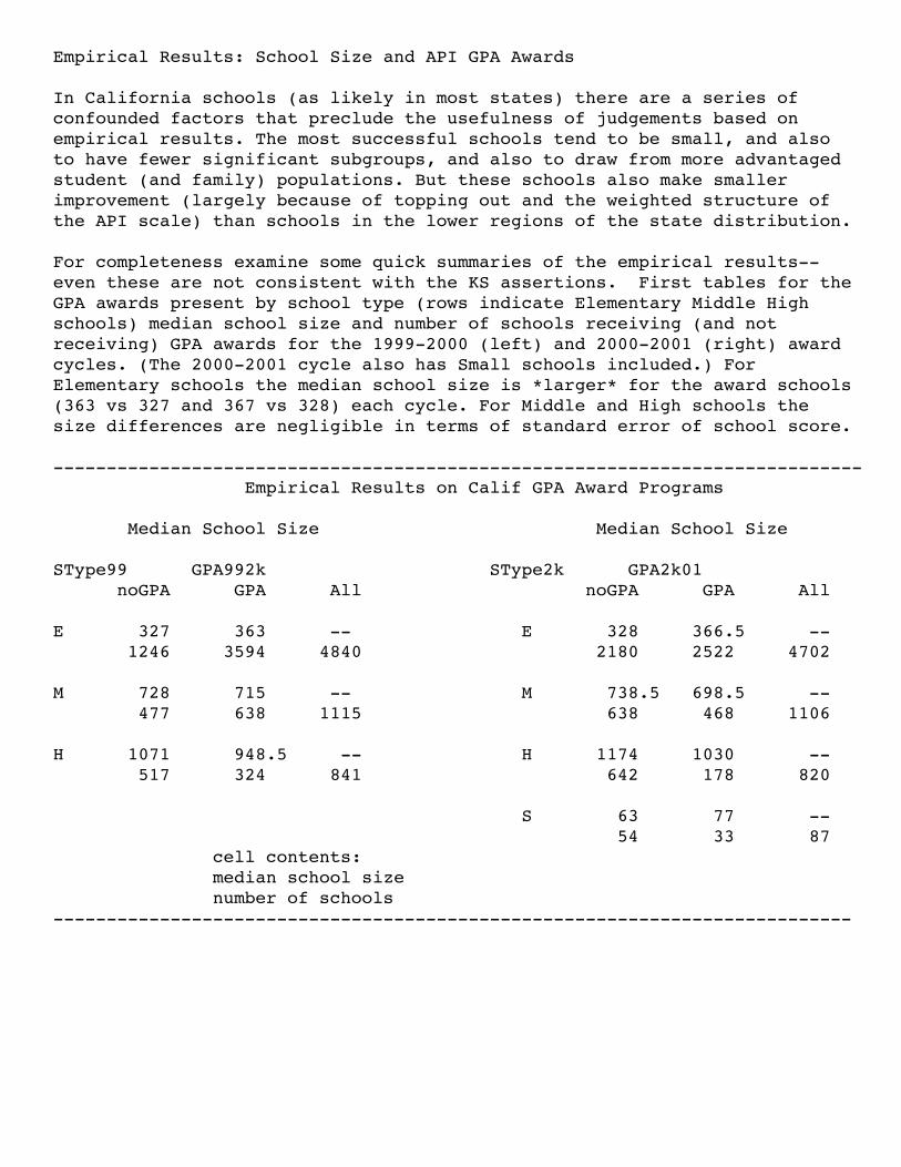
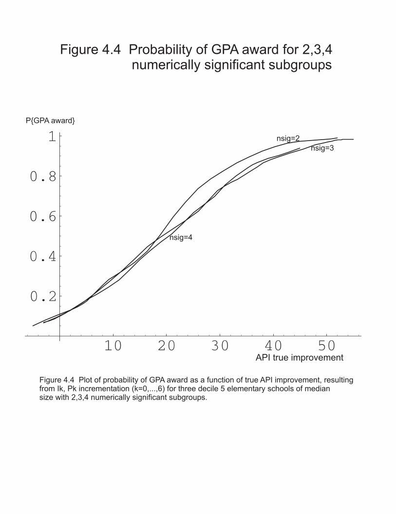
Figure 1.1 API Standard Errors ...................................... 20Figure 1.2 API State Decile Accuracy ................................ 23Figure 1.3 API Reliability Calculations ............................. 25Figure 2.1 Plots of Standard Error API Improvement versus Improvement ....................................... 34Figure 2.2 KS-style Plots of Improvement versus number of students .............................................. 36Figure 2.3 Plots for API Improvement Grade 3, Grade 4 Data .......... 38Figure 4.1 False Positive Probabilities and Standard Error API ...... 61Figure 4.2 Probability of GPA Award for Decile 5 Elementary Schools with nsig=3 ...................................... 64Figure 4.3 School Size and AB1114 Award Eligibility ................. 66Figure 4.4 Probability of GPA Award for 2,3,4 Numerically Significant Subgroups .................................... 70
Table 1.1 Accuracy Results for Grade-level Mean n=68 ................ 12Table 1.2 API Standard Errors--1999 Data ............................ 19Table 3.1 Consecutive Improvement for Artificial Three-Year Data (n=10000), Ex. A .......................................... 46Table 3.2 Consecutive Improvement for Artificial Three-Year Data (n=10000), Ex. B .......................................... 49Table 3.2 Consecutive Improvement for Artificial Three-Year Data (n=10000), Ex. C .......................................... 52Table 4.1 Probabilities of Award Eligibility and School Size: Four Elementary School Examples ........................... 58Table 4.2. Probabilities of GPA Award Eligibility and Number of Numerically Significant Subgroups ......................... 69[most tables are unnumbered and embedded in the text]
Irrelevance of Reliability Coefficients to Accountability Systems: Statistical Disconnect in Kane-Staiger "Volatility in School Test Scores"
David Rogosa Stanford University October 2002
PREAMBLE
In "Volatility in School Test Scores: Implications for Test-Based Accountability Systems" Kane and Staiger (hereafter KS) present lengthy empirical demonstrations and methodological prescriptions on the properties of accountability systems. The mission of this refutation is to persuade past and prospective readers of KS to disregard all but the most minor of their content (e.g., KS background exposition is quite good).
The accuracy of scores and, especially, the accuracy of decisions based on those scores are critically important topics: whether scores be from medical settings such as adult blood pressure or PSA measurements, or scores from high-stakes educational settings such as individual student test scores or group (e.g. school) composite summaries. And for the educational setting, the traditional tools from educational measurement or psychometrics for assessing the quality of measurements are for the most part inadequate or inappropriate for accountability systems. Concern should be focused on whether, or better how often, uncertainty in the scores can mislead in reporting or result in incorrect decisions. Accuracy can only be judged by reference to the purposes to which the data is put. And the most common mistake is to ask too much of the data (i.e., using the data to make distinctions that far exceed the accuracy of the data, as was done in the departed Kentucky accountability system based on KIRIS). To oversimplify, a yardstick (or tape-measure) has adequate accuracy for rough-cutting lumber or perhaps hanging kitchen cabinets, but is inadequate for neurosurgery or a LASIK procedure.
KS put forth both incorrect empirical assertions about Accountability Systems and unfortunate methodological standards and procedures for analyzing the properties of accountability systems. Both must be countered. For accountability systems (at state or national level) to be implemented and perhaps survive long-term, impressive obstacles--political, educational, practical, economic--must be overcome. The work here is motivated by the feeling that it would be a shame if those hurdles were overcome and yet the effort was blown due to failures of statistical work. My main referent for accountability systems is the system based on the California Academic Performance Index (API), which is also one the main examples in KS.
The technical analysis reveals that KS rediscover reliability coefficients (often without saying so explicitly) at almost every turn. Reliability coefficients for school-level scores address questions about relative standing (among schools) and individual differences (between schools). The statistical disconnect is that KS pursue questions about relative standing
even though that's not what accountability systems do. Reliability is not precision. Consequently, KS results and presentation have little relevance or useful implications for properties of accountability systems.
Letting KS speak for themselves, here are some representative assertions about accuracy of scores and accuracy of improvement:
We estimate that the confidence interval for the average fourth- grade reading or math score in a school with sixty-eight students per grade level would extend from roughly the 25th to the 75th percentile among schools of that size. Such volatility can wreak havoc in school accountability systems. (p.236)
many test-based accountability systems are relying upon unreliable measures. Schools differ little in their rate of change in test scores .... Moreover, those differences that do exist are often nonpersistent... we estimate that more than 70 percent of the variance in changes in test scores for any given school and grade is transient. For the median-size school, roughly half of the variation between schools in gain scores (or value-added) for any given grade is also nonpersistent. (p.239)
mean gain scores or annual changes in a school’s test score are measured remarkably unreliably. More than half (58 percent) of the variance among the smallest quintile of schools in mean gain scores is due to sampling variation and other nonpersistent factors. Among schools near the median size in North Carolina, nonpersistent factors are estimated to account for 49 percent of the variance. Changes in mean test scores from one year to the next are measured even more unreliably. More than three quarters (79 percent) of the variance in the annual change in mean test scores among the smallest quintile of schools is due to one-time, nonpersistent factors. Even though the largest quintile of schools was roughly four times as large as the smallest quintile, the proportion of the variance in annual changes due to nonpersistent factors declined only slightly, from 79 percent to 73 percent. (p.252)
The most important task is to demonstrate that the KS assertions are irrelevant to properties of accountability systems. A secondary concern, stimulated by the disparity between the empirical analyses for California API data (supplanted with analytic results) and the KS North Carolina results, is whether the demonstrably irrelevant KS calculations were even done correctly.
The body of this report consists of a fairly thorough effort to discredit the empirical assertions and methodological prescriptions in KS. The four main sections of content that follow this (lengthy) Preamble are:Section 1 Accuracy Of Group Summaries Exact results are obtained for the accuracy of grade-level scores (for n=68) which are then compared with the reliability-style calculations reported in KS for North Carolina data. Also, accuracy properties of California API school-level scores are presented, and to compare with KS assertions, the reliability coefficients for these scores are calculated. KS find high volatility even when accuracy is very good, and KS find extreme absence of volatility even when accuracy is moderate to poor. Section 2 Accuracy of Improvement Precision of improvement is contrasted with KS-style reliability of improvement. Analytic and empirical examples for accuracy of improvement reinforce the basic message: reliability is not precision. Most importantly, precision, which is what matters, can be low, and reliability still be high. And vice versa. Also, school-level California API data display no relation between amount of improvement and uncertainty in the scores (Figures 2.1-2.3), refuting a key KS assertion about school size.Section 3 Persistence of Change. The KS correlation of consecutive changes--and thus the KS estimate of "proportion of variance in changes due to nonpersistent factors"--is shown to be a function of the reliability of the difference score. KS determinations of persistence of change are shown to be without value in accountability systems. Common-sense definitions of consistency of improvement and empirical demonstrations using artificial data are presented.Section 4 California Academic Performance Index Award Programs Discussion of appropriate methods for describing the properties of Award Programs (e.g., determinations of false positive and false negatives) are contrasted with the incorrect empirical assertions and methodologies in KS. Counterexamples to each of the KS "Lessons" are presented in detail. The focus is on the effect of school size, to link with the accuracy results of previous sections.
Technical Caricature
For those familiar with the content of KS, the following small example captures much of the results demonstrating why KS should be set aside. By presenting an oversimplified caricature, there's always the danger in undermining the full argument, which does extensively use California data and detailed analytic results. But this caricature may be helpful in orienting readers to the key failings in KS and may help readers more readily absorb the more complex retelling of these points in the body of this piece. And some advanced readers may find that the caricature provides a convenient early exit point.
This artificial example seeks to highlight the distinction between statements about the relative standing of schools, which is what KS is about, and useful statements about performance and improvement of schools, which is what accountability systems, such as California's, are about. Adequate accuracy in statements about performance and improvement are
critically important (see my Plan and Preview document for the API). But, and this is the giant but, KS fatally err in using statements about relative standing-- reliability coefficients in transparent or disguised forms--to pronounce scores in the accountability systems volatile or imprecise. This caricature is an attempt to acclimate the reader to the conclusion of KS irrelevance, to be demonstrated with the empirical data throughout this report.
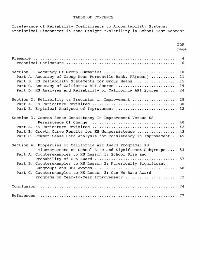
INSERT EXHIBIT 1
Column 1 of the caricature represents a single year cross-section, in which the accuracy of each school score is high, with scores around 500 and maximum error in the school scores of 2 points (60% chance of 1 point or less error). But because KS are concerned with relative standing, the KS methodology would find 1 - reliability = .5 and KS would pronounce the scores to be highly volatile. For KS 50% of score variation is due to error, and their explanatory vehicle of a confidence interval for the average school score extends from the 15th to 85th percentiles of the score distribution (probability score 497 or less, probability score 503 or more both equal .12).
Column 2 of the caricature considers year-to-year improvement. The scenario presents improvement of about 100 points, with the observed improvement pinned down reasonably accurately (probability .76 that the error in a school's observed improvement has magnitude 2 points or less). California citizens and California Department of Education would applaud a result of all schools gaining about 100 points with that observed improvement estimated with possible discrepancy of only a few points. Maybe even the LA Times would applaud. KS, however, would declare extreme volatility in the scores (85.7% of observed variance in gain due to error).
Column 3 moves on to consider KS questions of "persistence of change" over three years of observation. The scenario constructs perfectly persistent change (each school has the same true change time2 to time3 as time1 to time 2). Again the precision in estimating each school's change is good. However KS would declare over 50% of the variance in changes due to nonpersistent factors. The caricature result for KS of 4/7 of the variance in changes due to nonpersistent factors remarkably matches the KS empirical assertion "For the median-size school, roughly half of the variation between schools in gain scores (or value-added) for any given grade is also nonpersistent" (p.240).Additional asides for Column 3 results. First, notice the inconsistency in KS non-persistence. KS (column 2) would declare 85.7% of variance in time2 to time3 or time1 to time 2 is due to error, yet here in column 3 for the same data KS would declare only 57.1% of the variance in changes due to nonpersistent factors. Second, note that the reliability of time1 to time3 improvement is .4, and for this example 1 - reliability of time1 to time3 improvement (.6) is close to the KS proportion of the variance in changes due to nonpersistent factors (.571).
Collection of Schools
a. True measurements for thecollection of schools are distributedDiscrete Uniform [498, 502], i.e.,mass 1/5 at 498,..., 502. Underperfect measurement the schoolscores would have mean 500,variance 2.
b. error process obscuring the schoolscores are Discrete Uniform [-2, 2],i.e., mass 1/5 at -2, -1, 0, 1, 2. Errorvariance is 2 points.
c. The observed school scores havemagnitude around 500, and error isat most +/- 2 points. (Standard errorof the school mean is 1.41.) That mayseem a reasonably precise assessment.
d. KS would assert that 50% of theobserved variance due to error;scores would be considered"volatile".
Time 1
Exhibit 1KS Caricature
a. True improvement for each school isdrawn from Discrete Uniform [99, 101],mass 1/3 at 99, 100, 101.
b. The observed score for each schoolat time 2 is the sum of the time-1 truescore, true improvement, and a drawfrom the error process obscuring theschool scores: Discrete Uniform [-2, 2],i.e., mass 1/5 at -2, -1, 0, 1, 2.
c. The observed improvement is around100, with maximum error +/- 4 points(extremes attained with probability .04).
d. Reliability of time1-time2 differencescore is 1/7. Thus KS would assert thatover 85% of the observed variance inimprovement is due to error; improvementscores would be deemed extremely“volatile".
Time 2
a. True improvement for each school isidentical to the time1,time2 trueimprovement.
b. Observed score for each school attime 3 is the sum of the time-2 true score,true improvement, and a new draw fromthe error process obscuring the schoolscores: Discrete Uniform [-2, 2], i.e.,mass 1/5 at -2, -1, 0, 1, 2.
c. The observed time-2, time-3improvement is around 100.
d. KS compute the correlation coefficient,over schools, between time-2 minus time-1improvement and time-3 minus time-2improvement. KS assert that -2*correlationis "proportion of variance in changes dueto nonpersistent factors"
e. In this scenario true improvement foreach school is identical (perfectlypersistent) time-1 to time-2 and time-2 totime-3. KS would determine that over 50%(4/7) of the variance in changes due tononpersistent factors.
Time 3
[more technical details and discussion
in Section 2, part A]
[more technical details and discussion
in Section 3, part A]
[more technical details and
discussion in Section 1, part B]
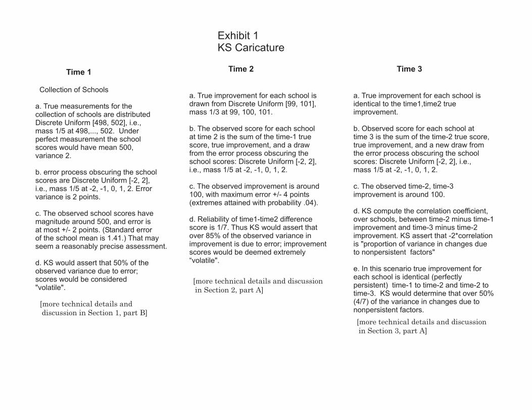
To repeat, the simple global statement is that accountability systems are not about relative standing determinations, and because KS is only about relative standing (reliability) determinations, KS is irrelevant. And irrelevance when propagated into methodology and policy is not benign; the consequence of irrelevance is serious misinformation. It would be bad enough if KS methods served to consistently understate the properties of accountability systems (i.e., large volatility everywhere), but the facts show that KS methods and results err in both directions.
As with most things in life, there's a 2x2 table that is useful. The table below "KS versus the Statistician" shows the four combinations of good/poor accuracy and high/low reliability (or equivalently low/high KS volatility). The cells in the table below indicate one example (often one of many). These examples are drawn from the content of Sections 1 and 2; similar arrays with different labels can be constructed for Sections 3 and 4 (e.g., for section 3, KS nonpersistence crossed with consistency of improvement).
KS versus the Statistician
Kane-Staiger Low Volatility High Volatility S (High Reliability) (Low Reliability)t _____________________________________________________a | t Good | High School Caricature examples;i Accuracy | API school score, or s | change in school scoret |i |c | i Poor | Fourth Grade Change in Fourtha Accuracy | API Grade APIn |
For example, consider the cell in which KS methods are far too optimistic: California API scores for fourth graders. California does not report API scores by grade level for good reasons, considering the relatively poor accuracy of these scores shown in Section 1, part C. Yet the reliability coefficient for grade 4 API is around .97 (see Section 1, part D), producing the KS determination of very low volatility, with 3% of variation in scores due to error.
SECTION 1 ACCURACY OF GROUP SUMMARIES
|------------------------------------------------------------------| | Train of Thought: Section 1 | |My attempt to avoid having the main argument washed away by the | |waves of technical detail and results is to precede each section | |with a short narrative. The setting is school scores (perhaps by | |grade level) in a single year. The main message is that KS methods| |err in both directions. As a consequence of irrelevance, KS | |methods find high volatility even when accuracy is very good, and | |KS methods find extreme absence of volatility even when accuracy | |is moderate to poor. | |Start out in part A by showing the actual statistical properties | |of a school score (taking the KS example of 68 fourth graders). | |Part B presents the KS methods for determining volatility: | |"percent of variation" due to error and a sort of a "confidence | |interval" measure. Both of these are reliability (relative | |standing) quantities, and neither is useful. The amount of | |uncertainty in grade-level scores is nowhere near what is implied | |by the KS North Carolina analyses. Column 1 of the KS Caricature | |is revisited as an example of scores with high accuracy that KS | |would term extremely volatile. Part C repeats part A in presenting| |the actual statistical (accuracy) properties for California API | |measures (school-level and a constructed grade 4 score). In Part D| |the KS methods are seen to determine that California scores have a| |stunning lack of volatility, even in the case of the grade 4 | |scores, which lack the accuracy to be usable (the reason | |California doesn't report grade level API). | |------------------------------------------------------------------|
The first topic to consider is the accuracy of a group summary for a singleschool (single grade-level or combined across grade levels) at a single year. KS use empirical information to make summary assertions (including assignations of "volatility") of the sort:
we would infer that 14 to 15 percent of the variation in fourth-grade math and reading test scores was due to sampling variation. p.241
We estimate that the confidence interval for the average fourth-grade reading or math score in a school with sixty-eight students per grade level would extend from roughly the 25th to the 75th percentile among schools of that size. p.236 Later in this section the proper interpretation and clear irrelevance of these types of statements will be explained. First, let's constructively address the question: How well do we pin down group summaries?
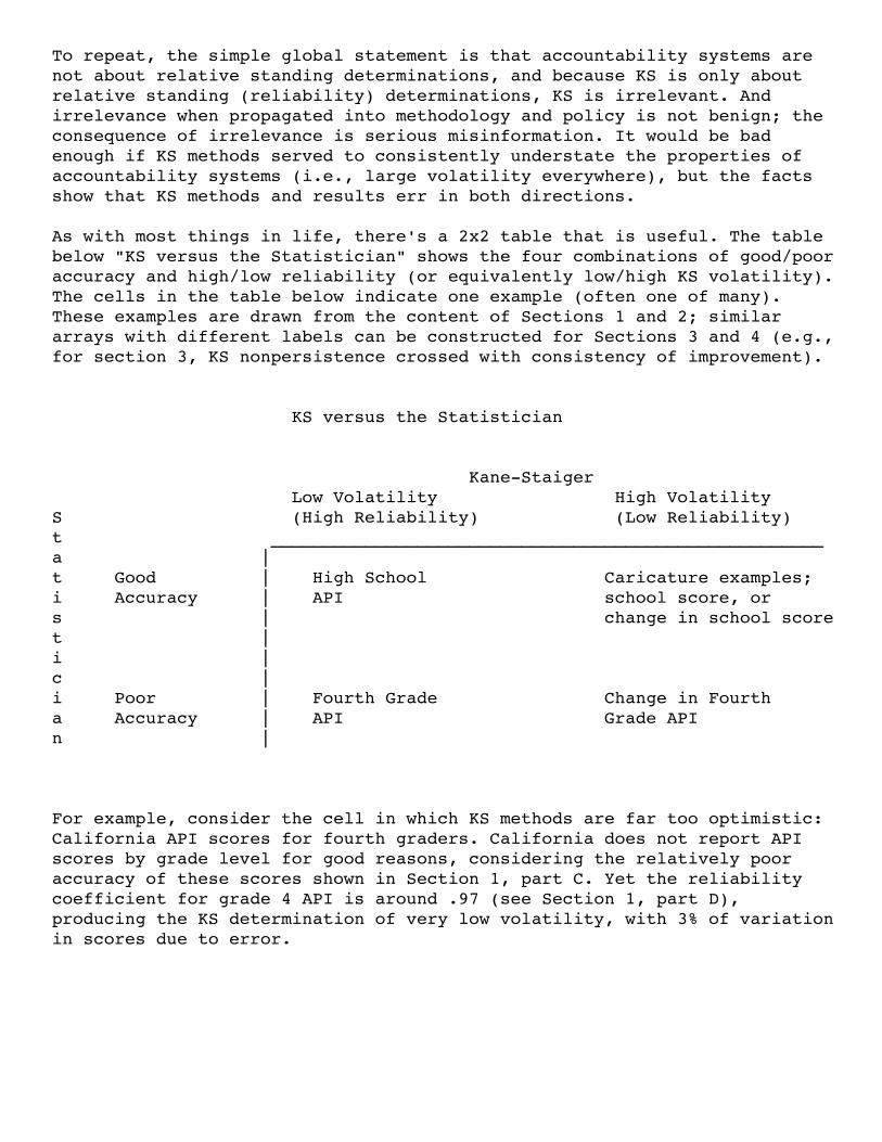
Section 1, part A. Accuracy of Group Mean Percentile Rank: PR[mean].
Statistical properties of PR[mean] are presented to illustrate useful information about the statistical properties of a group summary and to provide some sort of reality-check on the extensive KS presentation of the North Carolina data. PR[mean] is the individual percentile rank corresponding to the mean (scale) score for the group. PR[mean] is the featured type of group (school, district, state) summary measure reported to schools, districts, and the press by Harcourt Educational Measurement in California, and most test publishers also report this type of group summary. (A slight variation, the individual percentile rank corresponding to the mean normal curve equivalent score (nce) for the group, PR[mean(nce)], is equivalent to PR[mean] for the examples presented here.) A common informal explanation is "percentile rank for the average student". Attractive alternatives to PR[mean} are proportion above cut-off measures (PAC), and the California API is similar to a PAC (see Interpretive Notes API reports).
Taking the KS grade level example of n=68, Table 1.1 presents some useful examples of accuracy results. The group summary measure PR[mean] is explicitly described as: take the 68 scores on the grade 4 test (reading or math), average those scores (averaging scale scores is easiest to think in terms of) and obtain the percentile rank score in the individual norms distribution corresponding to the group mean. INSERT TABLE 1.1
Standard Error of PR[mean]The top frame of Table 1.1 presents the standard error for PR[mean], representing the statistical uncertainty in the PR[mean] score for 68 students. The 12 numerical values result from combination of two levels of test reliability, three levels of group mean, and two values of the group spread (psig). The two levels of typical full-form test reliability, reliabilities .9 and .95, show that these differences in test reliability (mainly a function of test length) have little consequence. Three different values of group mean percentile are shown (a group with relatively low mean at the 35th percentile, a group with mean at the 50th percentile, and a rather high group with mean at the 75th percentile), where the group mean percentile is most easily thought of as the value in the individual norms distribution resulting from perfect measurement on a infinitely large group (from which the n=68 are drawn). The value of psig is the ratio of the group standard deviation to the norming population standard deviation, so that psig = .9 roughly corresponds to a KS value of 81% of score variance being within-grades. For the approximately 5000 fourth-grades in California, about 30% of the score variance is between-schools, with median empirical psig value .84 (psig quartiles .76 and .91). One easy way of calibrating the true group mean and psig settings is through the resulting proportion at or above 50th percentile (PAC50): PAC50 values for Table 1 group specifications Group Mean psig = .8 psig = .9 Percentile .35 .315 .334 .5 .50 .50 .75 .800 .773
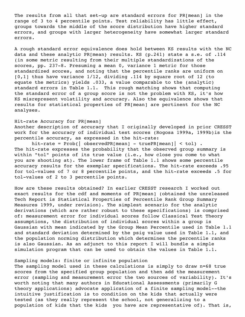
Table 1.1: Accuracy Results for Grade-level Mean n=68 Standard Error of PR[mean] for Grade-level Mean n=68
Test Reliability .90 Test Reliability .95 psig = .8 psig = .9 psig = .8 psig = .9 Group Mean Percentile .35 0.0368 0.0407 0.0363 0.0405 .5 0.0396 0.0438 0.0391 0.0435 .75 0.0316 0.0350 0.0312 0.0348 Percentile Accuracy of PR[mean] for Grade-level Mean n=68
Test Reliability .90 Test Reliability .95 psig = .9 psig = .8 tol .01 .03 .05 .08 tol .01 .03 .05 .08 Group Mean Percentile .35 0.192 0.534 0.777 0.949 0.216 0.589 0.830 0.972 .5 0.180 0.505 0.745 0.933 0.202 0.556 0.799 0.960 .75 0.222 0.598 0.838 0.974 0.248 0.658 0.888 0.988
The results from all that set-up are standard errors for PR[mean] in the range of 3 to 4 percentile points. Test reliability has little effect,groups towards the middle of the score distribution have higher standarderrors, and groups with larger heterogeneity have somewhat larger standarderrors.
A rough standard error equivalence does hold between KS results with the NC data and these analytic PR[mean} results. KS (p.241) state a s.e. of .114 (in some metric resulting from their multiple standardizations of the scores, pp. 237-8. Presuming a mean 0, variance 1 metric for those standardized scores, and noting that the percentile ranks are uniform on [0,1] thus have variance 1/12, dividing .114 by square root of 12 (to equate the metrics) yields .033, a value comparable to the (analytic) standard errors in Table 1.1. This rough matching shows that computingthe standard error of a group score is not the problem with KS, it's howKS misrepresent volatility and accuracy. Also the equivalence shows thatresults for statistical properties of PR[mean] are pertinent for the NCanalyses.
Hit-rate Accuracy for PR[mean]Another description of accuracy that I originally developed in prior CRESST work for the accuracy of individual test scores (Rogosa 1999a, 1999b)is the percentile accuracy, as expressed in the hit-rate: hit-rate = Prob{| observedPR[mean] - truePR[mean]| < tol} .The hit-rate expresses the probability that the observed group summary is within "tol" points of its true value (i.e., how close you come to what you are shooting at). The lower frame of Table 1.1 shows some percentileaccuracy results for the exemplar specifications. The hit-rate exceeds .95 for tol-values of 7 or 8 percentile points, and the hit-rate exceeds .5 for tol-values of 2 to 3 percentile points.
How are these results obtained? In earlier CRESST research I worked out exact results for the cdf and moments of PR[mean] (obtained the unreleased Tech Report is Statistical Properties of Percentile Rank Group Summary Measures 1999, under revision). The simplest scenario for the analytic derivations (which are rather robust to these specifications) is comprised of: measurement error for individual scores follow Classical Test Theory assumptions, the distribution of individual scores within a group is Gaussian with mean indicated by the Group Mean Percentile used in Table 1.1 and standard deviation determined by the psig value used in Table 1.1, and the population norming distribution which determines the percentile ranks is also Gaussian. As an adjunct to this report I will bundle a simple simulation program that can be used to obtain the values in Table 1.1.
Sampling models: finite or infinite population The sampling model used in these calculations is simply to draw n=68 true scores from the specified group population and then add the measurement error (sampling and measurement error the two sources of variability). It's worth noting that many authors in Educational Assessments (primarily G theory applications) advocate application of a finite sampling model--the intuitive justification is to condition on the kids that actually were tested (as they really represent the school, not generalizing to a population of kids that the kids you have are representative of). That is,
the argument for a finite population sampling model is that the specific students in the School or District (size N) constitute the population of interest. One example is the use of finite-sampling models in the G-component analyses of school scores conducted by the Superintendent's Select Committee (SSC) for the California Learning Assessment System data in 1994 (Cronbach et al,1994, Table 4, p.40). Additional discussion of the appropriateness of assuming a finite or infinite population sampling model can be found, with references, in Yen (1997). The relevance here is that under a finite sampling model, measurement error is the only source, and KS "volatility" would largely disappear (as sampling variance is their concern). The finite sampling argument is diminished by mobility and is more difficult to justify in year-to-year improvements. So this report, as does KS (cf KS pp.239-240), employs the infinite population results, as in these applications sampling from a large population of students does seem most appropriate.
To sum up, it is absolutely true that PR[mean] contains more statistical uncertainty than standard educational measurement techniques (Spearman-Brown etc) would imply. That's the reason I did the prior work, obtaining the standard error and other accuracy measures shown in Table 1.1 etc. The uncertainty in these scores has important policy implications. But the accuracy results demonstrate that the amount of uncertainty in the group measure is nowhere near what is implied by the KS "analysis" of the NC data. Furthermore, results in part B show good properties for this n=68 group summary measure even by the KS volatility criteria--the PR[mean] measure for n=68 has less (often far less) than ten percent of variation in scores due to "error" (sampling variation, measurement error).
Section 1, part B. KS Reliability Statements for Group Means
KS "Proportion of Variation" DeterminationsThe key, very basic, technical fact that translates KS statements intoreliability statements is boxed for easy (repeated) reference. _____________________________________________________________ | proportion of variance in group summary due to error = | | | | 1 - Reliability Coefficient(of group summary) | |____________________________________________________________|
In simplest terms a reliability coefficient is true variance divided by total variance, and as total variance is true variance plus error variance, reliability is often written as true/(true + error). In discussing some forms of the calculations, reference will be made to more formal technical versions of the basic variance decomposition, which can then be used for reliability coefficients, as in theorem 2.6.2 Lord and Novick (1968, sec 2.6, p.35, cf. p.61) or theorem 4.7 in Mood Graybill and Boes (1974, p. 159) on conditional and unconditional variances.
Turning to the KS statements for the North Carolina data, their statement for schools of average (n approximately 68) grade-level size: "14 to 15 percent of the variation in fourth-grade math and reading test scores was due to sampling variation" (p.241) is obtained from .15 = .013/.087 for reading and .14 = .013/.092 for math, where .013 is KS "estimated amount of variance due to sampling variation" and "the variance in mean reading and math scores was .087 and .092" (KS, p.241). Equivalently, KS are asserting that for average-sized fourth-grades, the reliability of the 4th grade reading score is .85 (.85 = 1 - .013/.087) and that the reliability of the 4th grade math score is .86 (.86 = 1 - .013/.092). The "percent of variation" statements throughout KS are reliability (relative standing) statements, not accuracy or precision statements.
The large point to be emphasized is that the KS analyses are reliability and relative standing statements and not relevant to Accountability Systems. Moreover, even within the KS realm of irrelevance internal consistency does not exist. On page 236, reliabilities of .86 are said to indicate "havoc wreaking volatility". Yet on p.251, in discussing Table 2, a reliability coefficient of .8 (for the smallest schools) yields the conclusion "a school’s average test performance in fourth grade can be measured reliably". The reader is spared the task of sorting out how reliability .8 yields "reliable" school scores, yet reliability .86 is "volatile" measurement by the simple guidance that both statements are best regarded as irrelevant to accountability systems.
KS "Confidence Interval" StatementsThe less obvious task is to translate the KS "confidence interval" statements into reliability statements. The KS CI statement which they employ "to gauge the importance of sampling variation" (p.241) is clearly intended for shock value, placed in their lead and then with more detail on p.241. Unless the reader proceeds carefully, the conclusion would be that a grade-level mean has a confidence interval that extends +/- 25 percentile points. However, Table 1.1 tells us that the probability is usually greater than .95 that the observed value of n=68 PR[mean] is within 8 percentile
points of its true value. The Table 1.1 results are accuracy statements about the precision of a school (grade-level) summary. On the other hand, the KS confidence interval is a reliability statement about relative standing.
To demonstrate that the KS confidence interval is just a restatement of a reliability coefficient requires a little detour. My way of calibrating reliability coefficients has been to express the reliability coefficient in terms of how many standard errors of measurements from the observed score mean to a specified observed score percentile, for a given level of reliability. The howmanysem function in Mathematica syntax howmanysem[rel_, uperc_] := Quantile[NormalDistribution[0, Sqrt[1/rel]], uperc]/Sqrt[(1 - rel)/rel]returns (for the classical test theory, Gaussian distribution setting) the number of standard errors between the mean of the observed distribution anda specified percentile (uperc) of the observed score distribution. Takingthe KS confidence interval statement, Among schools with between sixty-five and seventy-five students with valid test scores, such a confidence interval would extend from roughly the 25th to the 75th percentile. (p.241)howmanysem is set to 1.96, with a uperc of .75 implies a reliability coefficient .882. This .882 is a rather good match to the KS empirical reliability, value .86 obtained from the KS "percent of variance due to sampling variation" above. Or a reliability of .86 implies uperc .768, slightly above the 75th percentile; the exact match would be for n exactly 68 for a population of 4th grade scores that were Gaussian--given the roughness of the empirical distribution and variation in n for the NC data, this is a good match. The point here is that KS are merely presenting another reliability statement, not an accuracy statement, despite the camouflage of a confidence interval.
Furthermore, the KS confidence interval statement may not seem to be areasonable restatement of a reliability coefficient, as it is unflatteringeven for exceptionally high reliability of the group summary measure.-------------------------------------------------------------------------- reliability KS Confidence Interval 0.85 (0.224, 0.776) 0.90 (0.268, 0.732) 0.93 (0.302, 0.698) 0.95 (0.331, 0.669) 0.97 (0.367, 0.633) 0.98 (0.391, 0.609) 0.99 (0.422, 0.578)-------------------------------------------------------------------------- Volatility of PR[mean], aka Reliability Coefficient for PR[mean]. A calculation of a reliability coefficient for the PR[mean] group summary measure (which I hadn't done prior to these KS analyses) indicates that according to the KS criterion this group summary, even for n=68, would not be termed "volatile". To proceed with the calculation, KS p.420 indicate that for their North Carolina data the ratio of total variance to between-school variance is approximately 8. (This rather high value may be a result of the complex standardization of the scores pp. 237-8 or perhaps a property of the NC tests; CA 4th grades, see Part A, have a ratio closer to
3. The value for the reliability of PR[mean] is .905 for a population of n=68 schools (4th grades), with ratio of total variance to between-school variance 8 and test reliability .9. That's actually notably higher than the KS empirical estimates of approximately .86 (as no decrease in test reliability will reduce .905 below .894, even for test reliability less than .1). A less extreme value for ratio of total variance to between-school variance of 5 produces a value of .943 for rel(PR[mean]). To get down to a reliability of .86 for PR[mean] requires a value for ratio of total variance to between-school variance greater than 10. Thus for most reasonable configurations of group scores the "proportion of variation" due to error is well less than 10%.
KS Caricature, Column 1, Revisited.The artificial example in the Time 1 column of the KS Caricature in Exhibit 1 provides an even more vivid view of KS misstatements about accuracy and volatility. Start with a single year cross-section of perfectly measured school scores; "perfectly measured" says school scores with no statistical uncertainty, e.g. schools composed of an infinite number of students with student test scores obtained from very long tests. The error process obscuring the perfectly measured score is specified to be the same for each school (assumed for simplicity: think of all schools being the same finite size). The error process is Discrete Uniform [-2, 2]; that is, this error process has mass 1/5 at -2, -1, 0, 1, 2, and thus mean is 0 and error variance is 2 points.
In the KS formulation, the error variance arises from the heterogeneity of individual scores within a school--students within a school are seen as replications of the mean student (student scoring at the school mean) and all variability is seen as noise, giving rise to the standard formula for error variance of the school score: variance of student scores within a school divided by number of students (KS p.240). So the error variance of 2 points specified for a school score in the caricature could be mapped into a within-school variance of 200 points for the individual scores in a school of size 100. As KS indicate (p.239) their sampling model is student cohorts representing "a random draw from the population of students feeding a school" which is the sampling model mainly used for my results in this report. (The alternative finite sampling model described in part A, conditioning on the students that are tested, would yield far smaller standard errors for school scores.)
Thus in the caricature the standard error for a school score is 1.41,which appears small compared to the magnitude of the school score of 500.Accuracy of school score from the hit-rate criteria can be expressed as: P{observed school score is no more than 1 point different from the perfectly measured score} = .6, and P{observed school score is no more than 2 points different from the perfectly measured score} = 1.0.
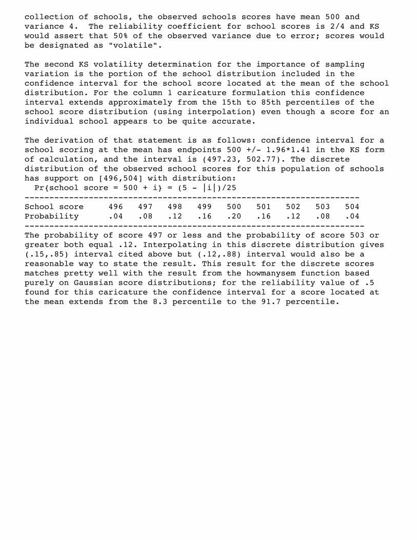
KS use different criteria than accuracy of a school score the for their assignation of volatility. Determinations of relative standing require specification of a population of schools: in column 1 caricature the distribution of true measurements for the collection of schools is Discrete Uniform [498, 502], i.e., mass 1/5 at 498,..., 502. Thus, under perfect measurement the school scores would have mean 500, variance 2. Over this
collection of schools, the observed schools scores have mean 500 and variance 4. The reliability coefficient for school scores is 2/4 and KS would assert that 50% of the observed variance due to error; scores would be designated as "volatile".
The second KS volatility determination for the importance of sampling variation is the portion of the school distribution included in the confidence interval for the school score located at the mean of the school distribution. For the column 1 caricature formulation this confidence interval extends approximately from the 15th to 85th percentiles of the school score distribution (using interpolation) even though a score for an individual school appears to be quite accurate.
The derivation of that statement is as follows: confidence interval for a school scoring at the mean has endpoints 500 +/- 1.96*1.41 in the KS form of calculation, and the interval is (497.23, 502.77). The discrete distribution of the observed school scores for this population of schools has support on [496,504] with distribution: Pr{school score = 500 + i} = (5 - |i|)/25 --------------------------------------------------------------------School score 496 497 498 499 500 501 502 503 504Probability .04 .08 .12 .16 .20 .16 .12 .08 .04---------------------------------------------------------------------The probability of score 497 or less and the probability of score 503 or greater both equal .12. Interpolating in this discrete distribution gives (.15,.85) interval cited above but (.12,.88) interval would also be a reasonable way to state the result. This result for the discrete scores matches pretty well with the result from the howmanysem function based purely on Gaussian score distributions; for the reliability value of .5 found for this caricature the confidence interval for a score located at the mean extends from the 8.3 percentile to the 91.7 percentile.
Section 1, part C. Accuracy of California API Scores
The purpose of this section is to provide a quick introduction to some statistical properties of the California API (c.f. "Plan and Preview for API Accuracy Reports"). The California API is the second main example in KS. The useful information on accuracy in this part C is then contrasted with KS analyses and results in part D. Readers not familiar with the API are directed to explanatory materials on the CDE website (www.cde.ca.gov).
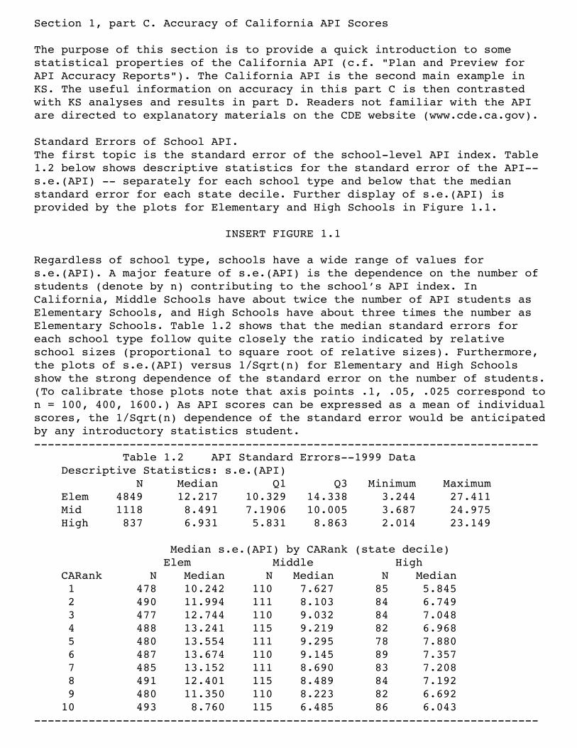
Standard Errors of School API. The first topic is the standard error of the school-level API index. Table 1.2 below shows descriptive statistics for the standard error of the API--s.e.(API) -- separately for each school type and below that the median standard error for each state decile. Further display of s.e.(API) is provided by the plots for Elementary and High Schools in Figure 1.1.
INSERT FIGURE 1.1 Regardless of school type, schools have a wide range of values for s.e.(API). A major feature of s.e.(API) is the dependence on the number of students (denote by n) contributing to the school’s API index. In California, Middle Schools have about twice the number of API students as Elementary Schools, and High Schools have about three times the number as Elementary Schools. Table 1.2 shows that the median standard errors for each school type follow quite closely the ratio indicated by relative school sizes (proportional to square root of relative sizes). Furthermore, the plots of s.e.(API) versus 1/Sqrt(n) for Elementary and High Schools show the strong dependence of the standard error on the number of students. (To calibrate those plots note that axis points .1, .05, .025 correspond to n = 100, 400, 1600.) As API scores can be expressed as a mean of individual scores, the 1/Sqrt(n) dependence of the standard error would be anticipated by any introductory statistics student.-------------------------------------------------------------------------- Table 1.2 API Standard Errors--1999 Data Descriptive Statistics: s.e.(API) N Median Q1 Q3 Minimum Maximum Elem 4849 12.217 10.329 14.338 3.244 27.411 Mid 1118 8.491 7.1906 10.005 3.687 24.975 High 837 6.931 5.831 8.863 2.014 23.149 Median s.e.(API) by CARank (state decile) Elem Middle High CARank N Median N Median N Median 1 478 10.242 110 7.627 85 5.845 2 490 11.994 111 8.103 84 6.749 3 477 12.744 110 9.032 84 7.048 4 488 13.241 115 9.219 82 6.968 5 480 13.554 111 9.295 78 7.880 6 487 13.674 110 9.145 89 7.357 7 485 13.152 111 8.690 83 7.208 8 491 12.401 115 8.489 84 7.192 9 480 11.350 110 8.223 82 6.692 10 493 8.760 115 6.485 86 6.043--------------------------------------------------------------------------
/
/
/
[ ]
[ ]
[ ]
1999 High Schools
1999 Elementary Schools
1999 Fourth Grades
Figure 1.1 API Standard Errors
Although the dependence of s.e.(API) on the number of students is strong, the plots also show some sizable differences for schools of the same size, mainly a result of the additional dependence of s.e.(API) on the school’s API score. The plots of s.e.(API) versus API show a pattern of larger s.e.(API) for API scores in the middle of the distribution, a pattern readers with an introductory statistics course will recognize as characteristic of a proportion score. (And readers of the Interpretive Notes series will recall the demonstrated correspondences between the API and proportion of students above the 50th and 25th national percentile ranks.) Similarly, in the portion of Table 1.2 displaying the median s.e.(API) by state decile, larger values of s.e.(API) are seen for schools in the middle deciles for each school type.
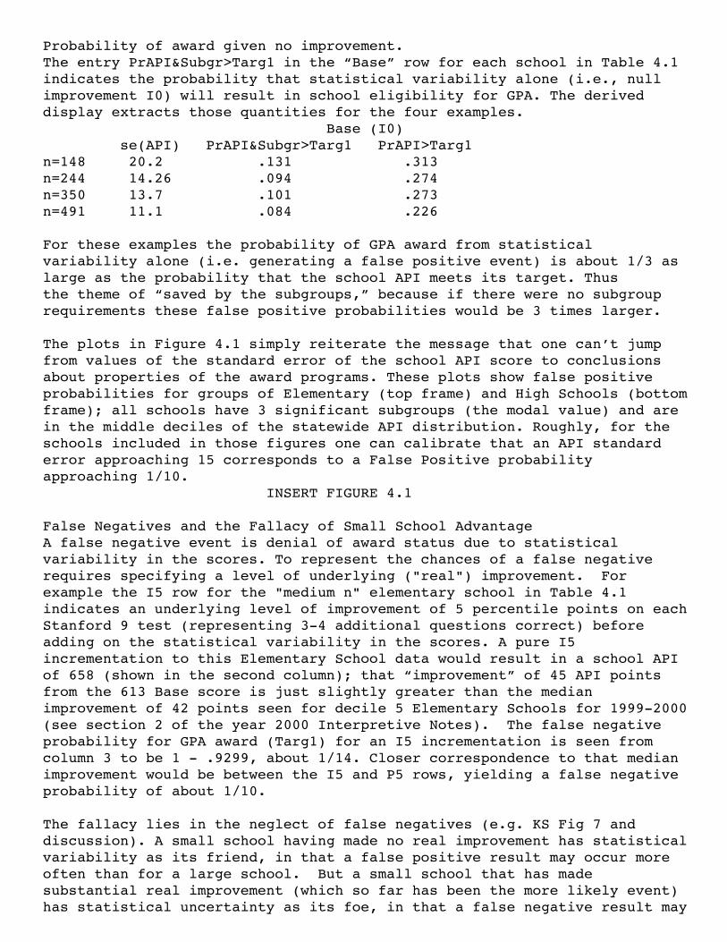
It is easy to see that school-level API scores do contain enough uncertainty that properties of award programs would be seen as unattractive if the award programs were based solely on the school API. But that's not how the California award programs are constructed (see Section 4, esp. Table 4.1, of this report and Plan and Preview document on the CDE site).
API scores for fourth graders.California does not present API scores by grade (for good reasons), but to answer the KS analyses of single grade-level data some corresponding analyses for California fourth-graders were conducted (with further use in part D). For the 1999 data, 4723 California Schools contributed more than 15 students (that threshold set to have at least a small classroom of 4th graders students in a school). Descriptive statistics for number of fourth-grade students in a school, fourth-grade API score, and standard error ofthe fourth-grade API score in those schools are:
4723 California Fourth Grades Variable Mean Median Q1 Q3 Minimum Maximum NAPI_99 83.959 79.000 58.000 103.000 16.000 379.000 CDEAPI_99 616.43 614.25 496.00 733.88 280.00 973.00 SEAPI99 26.721 25.792 21.558 30.769 5.622 70.861
The middle frames of Figure 1.1 which plot se(API) for the 4723 schools display a pattern similar to the school level scores, but with larger standard errors. The subset of 49 schools with exactly 68 fourth grade students provides some match to previous discussions of KS North Carolina results. For those schools with 68 fourth graders and having scores near the center of the score distribution, the standard error of the fourth-grade API is around 30.
Use these data to show a correspondence with Table 1.1 PR[mean} results in part A as follows. The API is on a 200-to-1000 scale, so to compare with PR[mean} on a 0-to-1 scale divide standard error of 30 by 800 to obtain .0375. This .0375 value is just slightly less than the .0391 for PR[mean] in Table 1.1 with psig = .8 (.0375 matches a school with "Mean Percentile" .5 and psig = .75). The message is that the standard errors for the various group summary indices are pretty much equivalent (simple behavior, no real surprises).
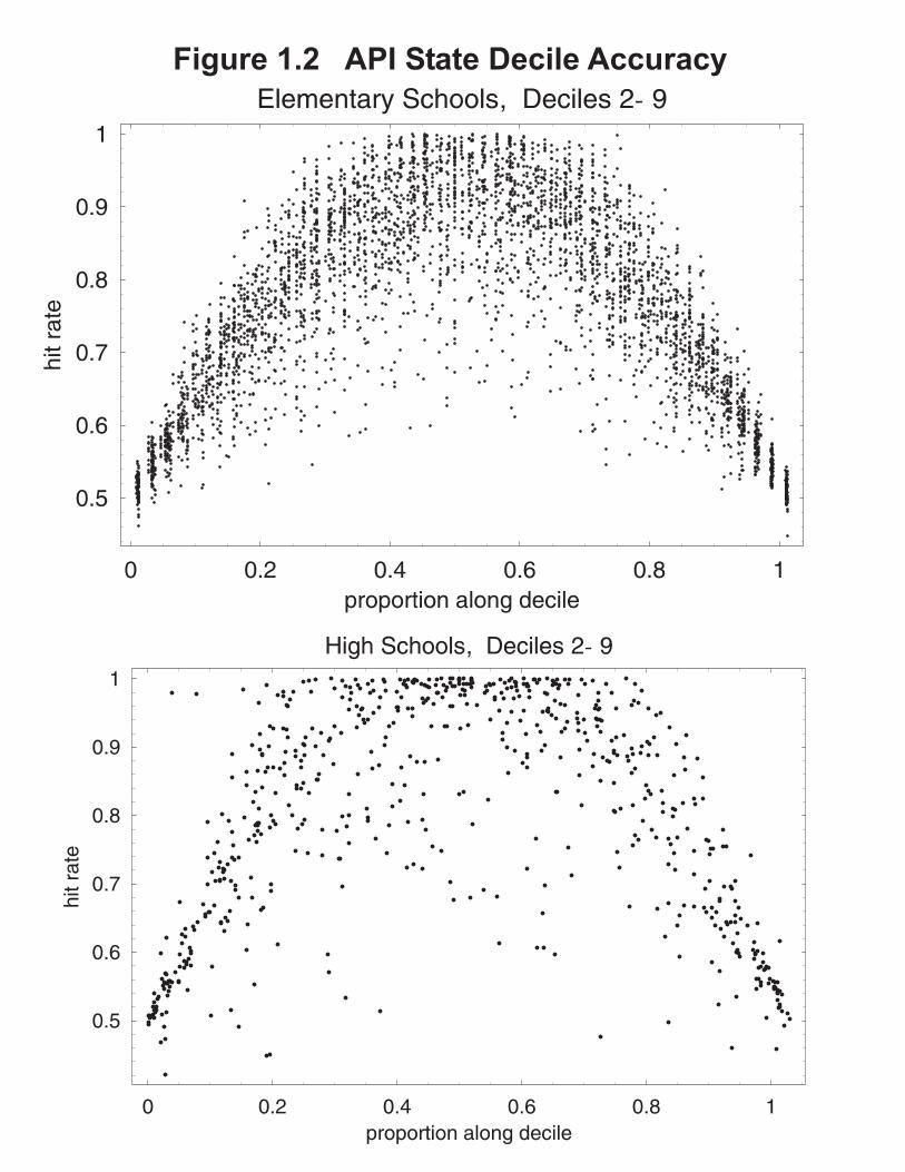
Decile Accuracy. There is one aspect in the California API reporting (but not award programs)that does have to do with relative standing of schools, the domain of KS.California reports a state decile (aka statewide rank) for the school APIscore as the obvious 1 (low) to 10 (top decile). So there is an aspect ofcomparing school scores to one another (relative standing) but the accuracyof these decile rankings is much greater than SK prose might imply.
The accuracy of the use of the school API score to determine the reported statewide rank is quantified by the hit-rate: decile accuracy hit-rate = 1 - Prob{sampling variability in API score moves the school out of its assigned decile}. The plots in Figure 1.2 show the hit rate for 1999 Elementary schools (top) and High Schools (bottom) in statewide deciles 2 through 9; the hit-rates are estimated from a bootstrap resampling. Of course, a school with an API score near a decile boundary will have a much larger probability of statistical variability moving it’s API score into a different decile; that’s what motivates plotting hit-rate versus position in the decile.
INSERT FIGURE 1.2
Schools in the middle of a decile have very high hit-rates (except for the smallest schools); almost all schools have resampling distributions contained within two adjoining deciles. The median hit-rate for Elementary schools is above .75 and for High Schools above .8. Median hit-rates broken down by state decile are given below; these numbers may calm a reader who had been spooked by the KS assertion of a confidence interval of plus or minus 25 percentile points (i.e. 5 deciles wide) for a school score in the North Carolina context.-------------------------------------------------------------------------- Median Decile Accuracy Hit Rates Elementary Schools High Schools Decile Median Hit-rate Decile Median Hit-rate 1 0.998 1 1. 2 0.787 2 0.974 3 0.786 3 0.888 4 0.762 4 0.773 5 0.751 5 0.808 6 0.725 6 0.778 7 0.777 7 0.787 8 0.798 8 0.837 9 0.888 9 0.889 10 1. 10 1.--------------------------------------------------------------------------
Figure 1.2 API State Decile Accuracy
Section 1, part D. KS Analyses and Reliability of California API Scores
It is easier to present and explain useful information on accuracy than to untangle and implement KS approaches. Notwithstanding, this part D develops the KS approach for the California API data. What we'll find is that KS indices vastly overstate the accuracy of the API scores; i.e., 'reliability is not precision' can work both ways. For median sized Elementary or High Schools less than one percent of the between school variance in API scores is attributable to error. Given those results the reader should wonder how Tom Kane can characterize the API scores in the national press as having "a lot of volatility" (LA Times Oct 16, 2001). The answer may lie in the even more flawed KS analyses taken up in Sections 2 and 3.
Calculation of API (school score) Reliability CoefficientThe s.e.(API) values for each school are the best descriptor of the accuracy of the API scores, but readers familiar with educational testing are conditioned to speak in terms of a reliability coefficient. Below is shown that even for a small elementary school (having s.e.(API) of nearly 20), the reliability of the API score exceeds .98. For readers not interested in the technical details of calculations for different sized schools, here's the simplest version. Take the set of 4849 Elementary Schools. The variance of the school API scores is 18728, and the mean of the API error variances (se(API)^2) is 169. Then a rough reliability coefficient is (18728 - 169)/18728 = .991 which translates for KS as less than one percent of variability in school API scores due to (sampling or measurement) error. (Results below confirm that .991 is a good descriptor of the reliability of the median-sized Elementary School.)
The approach to the reliability calculations is a rough educational testing analogy where n (number of students) serves the role of test length and, as in IRT situations, the error variance in the score also depends on the score level. What is shown in Figure 1.3 are fits to the plots of se(API) from Figure 1.1 using a simple quadratic for the fit of standard error on API score and a straight-line for standard error on 1/Sqrt[n]. (More sophisticated fits using smoothers won't change the gist of the results).
INSERT FIGURE 1.3 These fits then allow calculation of reliability coefficients for a population of schools of a specified size. The reliability coefficient can be expressed in a number of equivalent forms:
reliability = (observed variance - average error variance)/observed variance
The average error variance for a specified n was computed by integrating (averaging) the error variance functions displayed in Figure 1.3 over a "true score" distribution taken as Gaussian with observed score mean and variance computed as observed score variance minus overall average error variance. The observed variance is the sample variance for all included schools. (One could instead substitute the observed variance for the band of schools of similar size such as using the 552 Elementary schools of size 100 to 200 for the n=150 reliability calculation or the 692 Elementary schools of size 450 to 500 for the n=500 calculation; the largest effect on
the reliability calculations is the n=150 case where the reliability would change from .982 to .979.) A simpler approximation for the reliability of the average size school would be to substitute values for all schools into the reliability formula above--for the elementary schools (18958 -167.3)/18598 = .991 compared with .992 value for n=350 elementary schools.
The reliability coefficient for the API school score is presented for Elementary Schools, the separate Grade 4 scores, and High Schools, each for three values of school size (API n). In each case the middle row is the median size. Elementary Schools have quartiles of school size for API of 262 and 459, so the n-values of 150, 350 and 500 are roughly mid-lower quartile, median, mid-upper quartile. The High School n-values are approximately lower quartile, median, upper quartile of school size. For the Grade 4 scores the n=68 was chosen for the correspondence with the KS North Carolina discussion, and 103 is the 75th percentile of size.
-------------------------------------------------------------------------- API Reliability Coefficients
Elementary Schools Grade 4 High Schools n reliability n reliability n reliability150 0.982 68 0.965 500 0.991 350 0.992 79 0.970 1000 0.996 500 0.994 103 0.976 1500 0.997 --------------------------------------------------------------------------
Why is reliability of school scores so high (and thus KS volatility so low)? Relative standing assessments give great weight not to the accuracy of the scores, but to the ability to distinguish between low-scoring and high-scoring schools, a distinction that even rather inaccurate school scores cannot obscure.
The .965 value for grade 4 API reliability with n=68 is strikingly larger than the values of .85 obtained by KS for the North Carolina data. Furthermore, theoretical results in part B indicate reliability values around .95 for n=68 for a single test. Therefore it is rather hard to accept the KS empirical results at face value--unless the North Carolina tests have some truly strange properties, these discrepancies argue strongly that some aspect of the complex standardization described by KS produced artificially low reliability values. But such concerns are adigression from the main theme that the KS analyses aren't meaningful even if done correctly.
KS Confidence Interval. For completeness, here are some results for the KS "confidence interval" statement. The endpoints of a confidence interval for the average school score expressed as percentiles of the school score distribution. For California High schools the endpoints are the 45.7 and 54.8 (theoretical values from howmanysem in part B for reliability .996 are 45.1, 54.9). For the fourth grade scores the endpoints are the 38.9 and 62.9 (theoretical values from howmanysem in part B for reliability .965 are 35.7, 64.3). These fourth-grade results for this relative standing statement have half the interval-width claimed by KS from their NC analyses.
In sum, from these reliability results it would seem that California API scores should receive praise from KS for lack of volatility. Even in cases where the accuracy would/should be seen as relatively poor--the Grade 4 scores--KS criteria would find very good precision, as only 3 percent of between school variation is attributable to error. Whither volatility?
SECTION 2 RELIABILITY VS PRECISION IN IMPROVEMENT
|-------------------------------------------------------------------| | Train of thought: Section 2 | |Section 2 is in part a lead-in to Section 3, in which the main KS | |methodology on persistence of change is debunked. Also, Section 2 | |is somewhat of a continuation of Section 1--there's a "more of the | |same" theme in the contrasts between KS reliability determinations | |and useful measures of accuracy. But in Section 2 the score of | |interest is year-to-year improvement. Start with showing that KS | |statements about improvement are reliability statements. Next | |revisit the KS Caricature set-up to show that KS will find great | |volatility in the face of high accuracy. And then use California | |API data to compare accuracy in improvement with KS volatility | |determinations. KS methods err in both directions--high accuracy | |is volatility and lower accuracy is not. Also, KS assertions about | |statistical uncertainty in scores and amount of improvement are | |discredited in Figures 2.1-2.3. | |-------------------------------------------------------------------|
Again the basic problem with KS methodology is the focus on reliability and relative standing properties of the data--here with measures of improvement. Whether all schools improve by approximately the same amount is an interesting feature of the data to describe, but by no means does a lack of variability in improvement invalidate the accuracy of the measure of improvement. Again, the reliability coefficient for the measure of improvement does not reflect the accuracy of student or school improvement. Nor is that reliability relevant to the properties of an Accountability System based on "value-added". In KS own words, they use reliability measures:
the share of variance between schools in mean reading gain scores that is due to sampling variation is double that seen with mean reading score levels. Sampling variation makes it much harder to discern true differences in reading gain scores across schools.(p.242) by focusing on mean gains in test scores for students... many test-based accountability systems are relying upon unreliable measures. Schools differ little in their rate of change in test scores .... (p.239) mean gain scores or annual changes in a school’s test score are measured remarkably unreliably. (p.252)
Both KS methodology and empirical assertions must be discarded. This section establishes the obvious fact that KS methods for analyses of improvement are based on reliability measures, not accuracy determinations, and therefore should not be replicated by other researchers. But because KS emphatically conclude that the reliability properties of the accountability system data are not adequate, their empirical assertionsmust also be discredited.
KS are making reliability statements, in this context more directly than for single year scores in Section 1. To place the boxed statement from Section 1 in the time1, time2 improvement context:
_____________________________________________________________ | proportion of variance in improvement due to error = | | | | 1 - Reliability Coefficient of Difference Score | |____________________________________________________________|
Misunderstandings of the reliability of the difference score have a long history in Educational Measurement. The "reliability is not precision" theme in Rogosa et al (1982, pp.730-734 and Motto #6; cf Rogosa, 1995, Myth #2) tells the following story: high time1, time2 correlations between scores are taken as a prerequisite for stability, the consequence of which is diminution of individual differences in change, thus guaranteeing a small reliability coefficient for the difference score. That is, "you can't detect individual differences that don't exist." Therefore, a small reliability coefficient for the difference score does not imply lack of precision. Additional explanations of the reliability coefficient of the difference score are provided in Rogosa and Willett (1983).
Section 2, part A. KS Caricature Revisited.
Column 2 of the KS caricature displays one extreme example of reliability versus precision. Observed change with mean of 100 (values between 95 and 105) and standard error 2 points would appear to be accurately measured.P{observed change is no more than 2 points different from true change}=.76,P{observed change is no more than 3 points different from true change}=.92.However the reliability coefficient for observed change is paltry. The reliability of time1, time2 improvement is 1/7, or as KS would say, 85.7% of observed variance in gain is due to error (sampling variation).
Technical Details. The reliability value of 1/7 arises from the specification in the caricature that variance of true improvement (DiscreteUniform [99, 101]) is 2/3 and variance of observed improvement is 14/3 (see distribution below). The error in improvement is the difference between two independent discrete Uniform [-2, 2], each having mass 1/5 at -2, -1, 0, 1, 2. The probability distribution of the difference between the errors has support on [-4,4] with distribution Pr{error2 - error1 = i} = (5 - |i|)/25. Thus error2 - error1 has mean 0, variance 4. For observed change, the distribution, symmetric about 100, has the form:--------------------------------------------------------------------------- P{observed improvement = i}Observed 95 96 97 98 99 100Improvement 105 104 103 102 101
Probability .013 .04 .08 .12 .16 .173---------------------------------------------------------------------------From this discrete distribution the mean 0, variance 14/3 values used abovecan be confirmed.
Sampling Models: Matched, Unmatched, Partially matchedThis is a large topic which will be taken up more fully in a separate report. The example in the caricature pertains, for example, to year-to-year change for consecutive fourth-grades. That is, the calculation for variance of year-to-year change in school scores in the caricature assumes no overlap in the students in a school in year1 and year2. A completely matched sample would have, for example, all the students that are third-graders in a school in year1 become fourth-graders in that school in year2. A completely matched sample is obtained by KS through deleting about one-third of the NC student data (KS p.237). In most realistic settings, the partially matched samples case pertains. Mobility would indicate that not all third graders in year1 also constitute the fourth- graders for year2 in a school, and for school-wide scores, such as the California API, additional effects are that students in the top grade in year 1 are in a different school in year 2 and students in the lowest grade in year 2 were not present in year 1.
These different situations have consequence for the error variance for asingle school and for the reliability coefficient for the collection ofschools. Standard introductory statistics texts give the variance of time1,time2 change for the unmatched and completely matched cases. A simplederivation obtains the general case where "Povr" indicates the proportionof overlap--the ratio number of students present in the school both yearsto the number of students in year1 (assuming the same size both years).
For school scores indicated by Mean1 and Mean2 for years 1 and 2,within school variances indicated by Var1 and Var2, and the year1, year2and score correlation (for the population of students present both years)Corr12, and number of students in a year given by n, the variability of the year1 year 2 change (i.e. error variance for change) is given by
This formula reduces to the textbook results for Povr = 0 (unmatched) and Povr = 1 (completely matched). For the partially matched case it may be useful to think of Corr12*Povr as the "effective time1, time2 correlation".For the caricature formulation (in which Var1/n = Var2/n = 2), consider the following three cases.
Povr = 0. This unmatched case has been treated above with results: error variance for year1, year2 change for a school 4, resulting in reliability coefficient for year1, year2 change of 1/7 [2/3/(4 + 2/3)]. To obtain thevariance of 4, substitute into the formula above: Povr=0, and Var1/n = Var2/n = 2.
Povr = 1. This equally unrealistic case of perfectly matched year1, year2 student samples would produce a smaller value for error variance for year1, year2 change for a school. Using a Corr12 value of .75 the formula yieldsa variance of 1, and thus the standard error for a school's improvement is reduced from 2 points to 1 point. The reliability coefficient for change is 2/5 (up from the 1/7 in the unmatched case). But even in this limiting case KS would still determine 60% of variance in change due to error, even though the standard error of a school's observed change is only 1 point.(Note: the KS use of the formula with Povr=1 is seen in the arithmeticon p.242.)
Povr = 2/3. This value for partially matched year1, year2 scores is the same as KS in NC. The "effective correlation" is 1/2 and the formula yieldsa variance of 2. Thus the standard error for a school's improvement is 1.41 points. The reliability coefficient for change is 1/4 , and thus KS would determine 75% of variance in change due to error, even though the standard error of a school's observed change is only 1.41 points.
One small aside on KS misinformation. In their section "Schoolwide Scores, Overlapping Cohorts, and the Illusion of Stability" KS assert: considerable overlap exists in the sample of students in a school over a three-year period. Failing to take account of such overlap can create the illusion that school improvements are more stable than they are. (pp249-250)No! treating overlapping samples as if they were independent will inflate standard errors and diminish the apparent precision of change (and as seen above even diminish the associated reliability coefficient for improvement). The fable of the "stellar group of fourth graders" (p.250) notwithstanding.
In sum, careful consideration of these different sampling situations is important, but the basic point of the KS caricature pertains no matter whatthe configuration: in the face of very accurate determinations of time1, time2 improvement KS methodology would declare great volatility.
Section 2, part B Empirical Analyses of Improvement
KS NC Data Analysis
The KS empirical findings for North Carolina fourth-grade data stated by KS as "share of variance between schools in mean reading gain scores that is due to sampling variation is double that seen with mean reading score levels" implies the following arithmetic: proportion of variance in reading gain scores due to error is 2*.15 (where .15 was the proportion of variance in grade 4 reading scores due to error according to KS in Section 1). This is equivalent to a reliability coefficient for the difference score of around .70 (1 - 2*.15). That .7 reliability for a gain score is considerably higher than many in education are conditioned to seeing, and it's hard to understand how that result supports the incessant KS claim of debilitating volatility. [note: Here's my best attempt to reconstruct KS arithmetic: variance in within school gains (.343 in reading) divided by n=68 provides error variance .005 for gains. This also approximately matches .4*.013 obtained from substitution into the equation for Variance(Mean2 - Mean1) with Povr = 1 and Corr12 = .8. But the observed variance in reading gain is cited as .015, and the ratio .005/.015 = .333 implies a reliability for gain .67. Taking the verbal statement that "the between-school variance in mean student gains among schools of roughly the average size is only one-fifth as large as the between-school variance in mean fourth-grade scores" literally implies a value .087/5 = .0174 and .005/.0174 = .287 implying reliability for gain .713.]
California School-level API Scores
The California data can be used to rebut the various KS claims and also toprovide some useful information. The first data sets are API scores for 813 High Schools and 4737 Elementary Schools in 1999 and 2000. First off, estimated reliability coefficients for improvement in API are .863 for HighSchools and .804 for Elementary Schools. So much for the repeated KS claims"mean gain scores or annual changes in a school’s test score are measured remarkably unreliably. (p.252)" Wrong again. It's useful to deny KS anycredibility on empirical claims, but it's more important not to lose sightthat reliability coefficients aren't relevant for judging the properties of accountability systems.Calculation Details. The error variance for each school is computed fromthe Variance(Mean2 - Mean1) formula using the bootstrap standard errorsfor school scores as Sqrt[Var1/n] and Sqrt[Var2/n], Povr = 2/3, andCorr12 = .75. If instead, the unrealistic assumption of completely unmatched (no students present both years) the reliability values woulddiminish to .73 and .61. Reliabilities could be computed for different school sizes as was done in Section 1, part D; these reliability values apply to the median size school.
Turning to describing the improvement and accuracy in improvement, the table below gives percentiles for the collection of schools on the following quantities: observed improvement, standard error of improvement, and the coefficient of variation (CV) which is the ratio of the standard error to observed improvement. The standard errors of improvement are about the same magnitude as seen for the single year scores (see sec. 1, part C).
(Because of the induced complete matching in the KS NC subsample, standard errors of improvement were less than half as large as for the single year score.)--------------------------------------------------------------------- Improvement in API Scores High SchoolsPercentile Improvement Standard Error CV (se/imp)10 -12.125 4.97 0.16 20 -2.125 5.52 0.22 30 3.25 5.97 0.28 40 8.625 6.37 0.34 50 13.25 6.78 0.42 60 18.25 7.3 0.56 70 24.75 7.96 0.73 80 33.375 9.13 1.14 90 44.875 11.65 2.37
Elementary SchoolsPercentile Improvement Standard Error CV (se/imp) 10 4.562 8.67 0.16 20 15. 9.81 0.2 30 22.625 10.67 0.24 40 29.375 11.4 0.28 50 36. 12.13 0.33 60 42.75 12.83 0.39 70 51.188 13.68 0.5 80 61.25 14.76 0.71 90 75. 16.52 1.28 ---------------------------------------------------------------------The plots in Figure 2.1 show standard error of improvement vs improvement.Both this table and the Figure 2.1 indicate perhaps adequate, but far from outstanding accuracy in pinning down improvement.
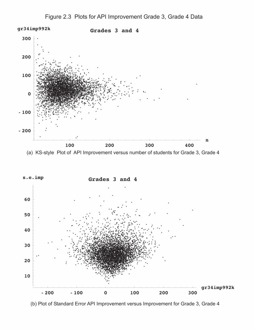
INSERT FIGURE 2.1
The plots in Figure 2.1 also debunk another main precept in KS, the KS attribution of statistical variation to explain a presumed relation between school size and of amount improvement. The KS reasoning seems to be that small schools will show more statistical variability (larger standard errors), so the biggest gainers and biggest losers both are likely to be small schools (as an artifact of statistical variability). For example, the section "Sampling Variation in Small and Large Schools" (p.242), KS Figure 3 and statements like "Test scores also fluctuate much more from year to year among small schools than among large schools."(p.245). This leads to their recommendation for accountability systems that as a consequence of the relation between statistical variability and amount of change (through the proxy of school size) different growth targets or different reward structures were needed for different size schools (KS Fig. 7, Lesson 1 in "Implications for the Design of Incentive Systems")
Fig 2.1 displays no discernable relation between amount of improvement and statistical uncertainty in improvement. Some non-gainers have big standard errors, some have small standard errors. Some large gainers have large standard errors, some have medium to small standard errors. Correlations
- 50 0 50 100 150 APIimp992k
5
10
15
20
25
s.e.imp Elementary Schools
- 50 - 25 0 25 50 75APIimp992k
5
10
15
20
s.e.imp High Schools
Figure 2.1 Plots of Standard Error API Improvement versus Improvement
between magnitude of change (absolute value) and standard error are .18 for High Schools and .19 for Elementary Schools. (Following the KS precept, the plots in Figure 2.1 would have something like a U shape, with large magnitude gains linked with large standard errors.)
As an adjunct, Figure 2.2 plots amount of improvement versus school size which does show the kind of funnel shape that KS emphasized in previous work (Kane and Staiger, “Improving School Accountability Measures,” esp their Figure 1 change in score vs school size for 5th gr math and reading). Note, for amusement, that the largest Elementary School in Figure 2.2 shows one of the largest gains (nearly 100 points) as a counterexample to the KS assertion "large schools have little chance of ever achieving the extremes" (p.256). Whatever relation might be discerned between amount of change and school size is due to factors (perhaps real school organizational effects) other than statistical variability. The larger message, which appears throughout Section 4, is that statistical properties of scores can't be inferred indirectly from observed patterns of school scores (here by KS plot gain vs n) which depend on a variety of confounded factors and real educational effects. Instead, statistical properties need to directly investigated, as in actual computations of standard errors, or in Section 4 probabilities of false diagnosis.
INSERT FIGURE 2.2 California Grade-level API Scores
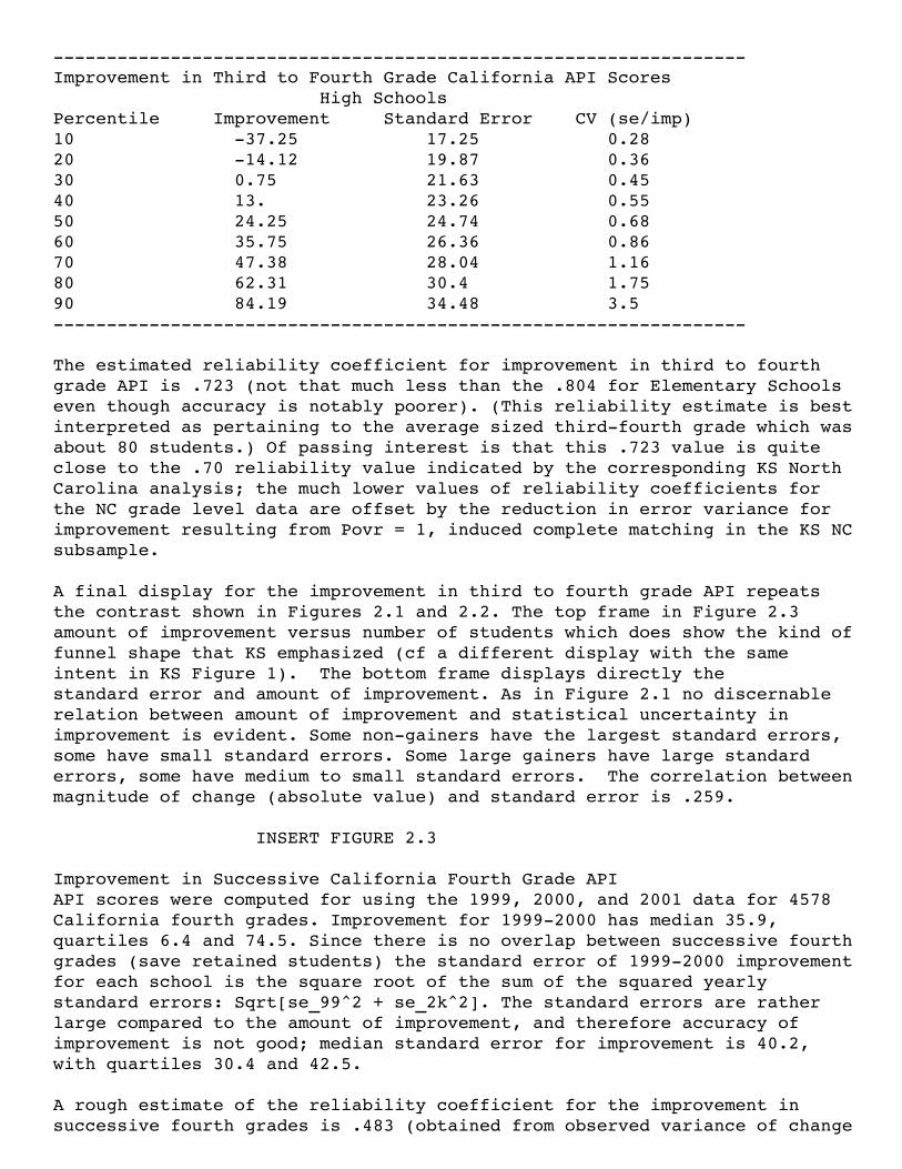
The following provides another good illustration of why California does not report grade-by-grade API scores. The first example, to mirror the KS presentation pp.242-244 for North Carolina data, is improvement in California API scores for third graders in the first year and corresponding fourth graders the second year. This is a partial overlap case where not all third graders in year 1 are fourth graders in the same school in year 2 (cohort partially replicated). The second example is successive fourth grade scores (with no overlap of students).
Improvement in Third to Fourth Grade California APIFor each of 4502 California schools an API score was computed for third graders in 1999 and fourth graders in 2000. The improvement measure for each school is then the year 2000 Grade 4 API minus the year 1999 Grade 3 API. Standard errors for each of those yearly scores were obtained from bootstrap resampling. Standard error for improvement was calculated fromthe Variance(Mean2 - Mean1) formula using the bootstrap standard errorsfor school scores as Sqrt[Var1/n] and Sqrt[Var2/n], Povr = 2/3, andCorr12 = .75. (The induced complete matching in the KS NC subsample makestheir Povr = 1.)
The table below gives some accuracy information, percentiles for the collection of schools on the following quantities: observed improvement, standard error of improvement, and the coefficient of variation (CV, the ratio of the standard error to observed improvement). Accuracy is not nearly as good as year-to-year improvement for Elementary Schools (for which accuracy was not great).
500 1000 1500 2000 2500 3000n
- 50
- 25
25
50
75
APIimp992k High Schools
200 400 600 800 1000 1200 1400 1600n
- 50
50
100
150
APIimp992k Elementary Schools
Figure 2.2 KS-style Plots of Improvement versus number of students
-----------------------------------------------------------------Improvement in Third to Fourth Grade California API Scores High SchoolsPercentile Improvement Standard Error CV (se/imp)10 -37.25 17.25 0.28 20 -14.12 19.87 0.36 30 0.75 21.63 0.45 40 13. 23.26 0.55 50 24.25 24.74 0.68 60 35.75 26.36 0.86 70 47.38 28.04 1.16 80 62.31 30.4 1.75 90 84.19 34.48 3.5 -----------------------------------------------------------------
The estimated reliability coefficient for improvement in third to fourth grade API is .723 (not that much less than the .804 for Elementary Schools even though accuracy is notably poorer). (This reliability estimate is best interpreted as pertaining to the average sized third-fourth grade which was about 80 students.) Of passing interest is that this .723 value is quite close to the .70 reliability value indicated by the corresponding KS North Carolina analysis; the much lower values of reliability coefficients for the NC grade level data are offset by the reduction in error variance for improvement resulting from Povr = 1, induced complete matching in the KS NC subsample.
A final display for the improvement in third to fourth grade API repeats the contrast shown in Figures 2.1 and 2.2. The top frame in Figure 2.3 amount of improvement versus number of students which does show the kind of funnel shape that KS emphasized (cf a different display with the same intent in KS Figure 1). The bottom frame displays directly the standard error and amount of improvement. As in Figure 2.1 no discernable relation between amount of improvement and statistical uncertainty in improvement is evident. Some non-gainers have the largest standard errors, some have small standard errors. Some large gainers have large standard errors, some have medium to small standard errors. The correlation between magnitude of change (absolute value) and standard error is .259.
INSERT FIGURE 2.3 Improvement in Successive California Fourth Grade APIAPI scores were computed for using the 1999, 2000, and 2001 data for 4578 California fourth grades. Improvement for 1999-2000 has median 35.9, quartiles 6.4 and 74.5. Since there is no overlap between successive fourth grades (save retained students) the standard error of 1999-2000 improvement for each school is the square root of the sum of the squared yearly standard errors: Sqrt[se_99^2 + se_2k^2]. The standard errors are rather large compared to the amount of improvement, and therefore accuracy of improvement is not good; median standard error for improvement is 40.2, with quartiles 30.4 and 42.5.
A rough estimate of the reliability coefficient for the improvement in successive fourth grades is .483 (obtained from observed variance of change
- 200 - 100 0 100 200 300gr34imp992k
10
20
30
40
50
60
s.e.imp Grades 3 and 4
Figure 2.3 Plots for API Improvement Grade 3, Grade 4 Data
(b) Plot of Standard Error API Improvement versus Improvement for Grade 3, Grade 4
(a) KS-style Plot of API Improvement versus number of students for Grade 3, Grade 4
100 200 300 400n
- 200
- 100
0
100
200
300
gr34imp992k Grades 3 and 4
minus average error variance of change all divided by observed variance of change). This reliability estimate is best interpreted as pertaining to the average sized fourth grade which was about 80 students (see Part 1C). (Theanalyses of Part 1D, e.g. Fig 1.3, providing reliability estimates fordifferent school sizes could be replicated here.)
SECTION 3 COMMON SENSE CONSISTENCY IN IMPROVEMENT VERSUS KS PERSISTENCE OF CHANGE ______________________________________________________________________ | Train of thought: Section 3 | |The main KS methodological tool is their estimate of "proportion | |of variance in changes due to nonpersistent factors". Show that the | |KS estimate turns out to be the (irrelevant) reliability of the | |difference score. Strong consistency in improvement will be labeled | |as "nonpersistent" or "transient" by KS. And vice versa. Finish up | |by showing some useful data analysis for consistency in improvement.| |____________________________________________________________________|
In their section "A Measure of the Persistence of Change in School Test Scores" (starting p.245) develop statistical procedures to estimate "the proportion of the change in test scores that is attributable to nonpersistent factors." (p.247) An example of the results produced by this method are the assertions (p.239)
Schools differ little in their rate of change in test scores ... Moreover, those differences that do exist are often nonpersistent— either because of sampling variation or other causes. For instance, we estimate that more than 70 percent of the variance in changes in test scores for any given school and grade is transient. For the median-size school, roughly half of the variation between schools in gain scores (or value-added) for any given grade is also nonpersistent.
This section demonstrates that the KS statistical procedures for determinations of "transient" (or the apparent synonym "nonpersistent") change are without value, and that the conclusions based on their procedure can be wildly misleading. In addition, the constructive content in this section explains and illustrates common-sense data analysis approaches to consistency of improvement.
KS procedure for "Persistence of Change"The KS procedure uses three successive years of data from non-overlapping samples--e.g. fourth grade scores for three years. A correlation coefficient between two difference scores, year2 minus year1 and year3 minus year2, is computed. Multiply that correlation by -2 to obtain "the proportion of the change in test scores that is attributable to nonpersistent factors."(p.247). In their own words "given an estimate of the correlation in changes in test scores in two consecutive years, we can estimate the proportion of the variance in changes that is due to nonpersistent factors by multiplying that correlation by –2." With "beautiful weather" and "barking dogs" as their technical guideposts KS explain: "If the correlation were zero, we would infer that the changes that occur are persistent. If the correlation were close to –.5, we would infer that nearly 100 percent of the changes that occur are purely transitory, such as sampling variation or a dog barking in the parking lot on the day of the test or inclement weather."(p.247).
KS present empirical results for this procedure in their Figure 4 ,"Correlation in the Change in Scores in Consecutive Years by Size of School in North Carolina and California". A separate correlation is computed for each quintile of school size (i.e. smallest fifth of schools to largest fifth). KS assert:
In North Carolina, the correlations ranged between –.25 and –.4. Using the reasoning above, this would imply that between 50 and 80 percent of the variance in the change in mean fourth-grade scores is nonpersistent. If one were to look for signs of improvement by closely tracking changes in mean scores from one year to the next, 50 to 80 percent of what one observed would be temporary—either due to sampling variation or some other nonpersistent cause. (p.248)
KS are saying rather clearly that they can determine that the school improvement that is observed is not real--i.e. due to error. Gains seen one year will disappear the next because the gains are transient. These KS determinations would be very important, and very discouraging, for educational assessment and educational policy if the KS procedures were plausible and the results credible. The purpose of this section is shout: Not so!
California, according to KS, is even worse. Almost all improvement isfound to be transient or "fleeting":
For the smallest fifth of schools, the correlation in the change in adjacent years was –.43, implying that 86 percent of the variance in the changes between any two years is fleeting. For the largest fifth of schools, the correlation was –.36, implying that 72 percent of the variance in the change was nonpersistent. p.249
The main technical result of this section, discussed in part B and Exhibit 2, is that under perfect consistency of true improvement:
_____________________________________________________________ | KS proportion of the change in test scores that is | | attributable to nonpersistent factors = | | | | 1 - 3*Reliability Coefficient of Difference Score | |____________________________________________________________|
Yes, the reliability coefficient for the difference score is once again, unbeknownst to KS, front-and-center in KS analyses. (Details and derivation are in part B and Exhibit 2; the simplest formulation in the box has the reliability of difference score the same from time1 to time2 as for time2 to time3).
Not expectedly, the demonstrations of this section are that KS find persistence when there is little consistency and volatility in the presence of great consistency. KS methods do not provide useful information, and that's a conclusion that does persist over time and over topics.
Section 3, part A. KS Caricature Revisited.
The KS Caricature (see Exhibit 1) result that 4/7 (57%) of change is attributable to nonpersistent factors closely matches the KS empirical conclusion for a median-size North Carolina fourth grade. The caricature is set up to have maximal persistence of change in that each unit (school) has a true change (99, 100, or 101 points) that is identical time1 to time2 and time2 to time3. And in the caricature formulation change is measured accurately. The caricature serves as one counterexample to the KS procedure; even with perfect consistency in true improvement and accuratemeasurement of improvement, KS determines 57% of change transient. Go figure.
The caricature points up an interesting inconsistency in KS non-persistence. In Section 2 setting KS would use the time1-time2 reliability coefficient for the difference score to declare 85.7% of variance in time1 to time 2 improvement due to error (same for time2 to time3). Yet for the same structure KS would declare only 57.1% of the variance in changes due to nonpersistent factors. (i.e. one would expect that persistence of change is a tougher criteria than just change, not the reverse). Actually, when there is consistency in improvement, this KS inconsistency between the nonpersistence measure and proportion variance due to error will be large.
As noted in the discussion of the caricature in the Introduction, the reliability coefficient for time1 to time3 improvement is .4, and 1 -.4 = .6 would serve in terms of KS Section 2 discussion to be the proportion of variance in change due to error. In this particular caricature formulation, this .6 value is quite close to the KS nonpersistence value .571, as will be the case when the reliability coefficient for time1, time2 change is very small (<.2). Yet another reliability coefficient interpretation for the KS analysis.
One interesting variation on the caricature formulation is to allow for deceleration. For example, for each unit true improvement from time2 to time3 is a proportion h (h<1) of the true improvement time1 to time2. The caricature has h=1. For example, h=.5 would have true improvement around 50 points for time2 to time3. The table below shows that h=.5 would increase the reported proportion nonpersistent by KS from .57 to .76.--------------------------------------------------------------------------- h .1 .2 .3 .4 .5 .6 .7 .8 .9 1.KSprop 0.89 0.86 0.83 0.79 0.76 0.72 0.68 0.65 0.61 0.57---------------------------------------------------------------------------
Technical note, overlap.The concern about overlap of students contributing to school scores in both time1 and time2 in Section 2, which translates into correlated errors over time for scores in the caricature, is not present in the persistence of change setting because KS develop this procedure for successive cohorts. Therefore the technical details of computing variances and covariances discussed in Section 2 are not needed here. In their own words, KS explain: "We can estimate the amount of variation due to sampling variation by assuming that the succession of cohorts within a particular grade is analogous to a random sampling process." (p.246)
Section 3, part B. Growth Curve Results for KS Nonpersistence
The main content is contained in Exhibit 2. The purpose is to understand the properties of the KS proposed statistic: -2*KSrho in the notation of Exhibit 2. The setting in Exhibit 2 specifies consistency in true improvement which is obscured by error of measurement (for the school setting this error of measurement is a surrogate for the statistical variability in the school score, single or multiple grades). Do the conclusions indicated by the KS statistic reflect the structure of the data?
The constant rate of change model in item 1 is a special case of the proportional deceleration in item 2 with h=1. Other models, such as proportional or exponential growth, could be used for these same purposes.
INSERT EXHIBIT 2 The primary message of Exhibit 2 is that the KS statistic for persistence of change represents another use by KS of the gain score reliability coefficient (the topic of Section 2). These results make it all too easy to create examples with any properties desired: combine good or poor accuracy with consistency of improvement to produce KS conclusions of either strong persistence of change or no persistence of change. It can go either way.
For example, Exhibit 2 shows how to obtain perfect KS persistence of change (i.e., 0% transient) with reliability of the time1, time2 difference score of 1/3 and h=1 or reliability of the time1, time2 difference score of 2/5 and h = 3/4 or reliability of the time1, time2 difference score of 1/2 and h = 1/2. Low values of the reliability of the time1,time2 difference score can be constructed either with very accurate measurement and little individual differences in change or with poor measurement (low accuracy) and large individual differences in change. On the other hand, very good accuracy for estimating change and perfect consistency of true change can lead to a KS determination that a large proportion of change is transient. The caricature provides one example; additional examples are left as an exercise for the reader. So it seems little can be learned, but much misinformation generated, from computing the KS statistic.
Furthermore, the KS persistence statistic has a counter-intuitive relation to other KS volatility measures, and the statistic reacts strongly to small changes in the reliability of time1, time2 gain. As is shown in Exhibit B for h=1, a .3 value for the reliability of time1,time2 gain produces a result worth celebrating--only 10% of change transient. Yet KS would also assert 70% of variation in time1, time2 scores due to error and proclaim disastrous volatility. If instead the reliability of time1,time2 gain were reduced from .3 to .2 then 40% of change is termed transient (yet 80% of time1,time2 variation due to error).
Exhibit 2 Mathematical Results for Persistence of Change
1. Constant Rate of Change
2. Proportional Deceleration in Change
Data on 3 observations, times 1,2,3, observed score on unit at time Xts
KS correlation KSrho = Corr[X2s_
X1s, X3s_
X2s ]
s t
Each unit s has true change and the constant rate of change model is
where the perfectly measured score for unit s at time t is (0) + t and the error of measurement
has measurement error variance
�
� � �
� �
s
s s
X (t) = (0) + t +s s s ts� � �
�
Brute force substitution (using errors independent because no overlap among successive years)
produces the result KSrho = [Var( ) _ Var( )] [Var( ) + 2Var( )] and the reliability of the difference
score Dt = Xt+1_ Xt is (D ) =
�
� � � �
�
/
t Var( )/[Var( ) + 2Var( )]. Then the relation is KSrho = [3 (D) 1]/2
and for the proportion nonpersistent measure: 2*KSrho = 1_
3 (D) .
� � � �
� �
-
A modified constant rate of change model, which may better reflect empirical experience in state
assessments, has school scores increasing smaller amounts in successive time periods. That is,
X (t+1) X (t) = ht-1 + ( ) for 0 < h < 1 (e.g., h=.5), which simply says that the true
improvement between times 1 and 2 is and between times 2 and 3 is h . Then for the
which can be put fully in terms of the time1-time2
reliability of the difference score by substituting
(D ) = h (D ) [1 (D )(1 h )] . The
plot at the right shows values for 2*KSrho.
2 1
1
1 1
2 2
2 2
2 2
2
/
/
½
0.3 0.4 0.5 0.6 0.7 0.8 0.9 1
-0.75
-0.5
-0.25
0
0.25
0.5
0.75
1
Plot of KS proportion nonpersistent as afunction of h for values of (D )� 1
(D ) values� 1
.1
.2
.3
.4
.5
.6
h
�2*KSrho
Section 3, part C. Common Sense Data Analysis for Consistency in Improvement
In California, one aspect of the ongoing debate on accountability systems was the contention, put forth by the California Teachers Association and others, that year-to-year improvement in API scores was well-described by a "see-saw" metaphor in that schools with scores that showed strong gains (and achieved awards) in one two-year cycle reversed those gains in the succeeding two-year cycle. This represents an empirical conjecture about consistency in improvement. For California data analysis addressing those concerns refer to reports on the API Research page: "Year 2001 Growth Update: Interpretive Notes for the Academic Performance Index" and "Analyses of AB1114 Schools". Those data analysis strategies (e.g., displays of the form of Tables 3.1 and 3.2) are used here to further illustrate the deficiencies of the KS statistic for persistence of change.
In the context of the stock market, the requisite wisdom is provided by Art Cashin, from UBS Paine Webber and ubiquitous on CNBC etc, who states the criterion for the credibility of a (short-term) stock market rally as: "Don't give up your gains." That motto seems also to be prescriptive for investigation of consistency of improvement in school accountability indices.
Example A: Large KS NonpersistenceThe first example for describing consistency in improvement (Example A) is composed of observations on 10000 units (e.g., schools) on three consecutive time points, e.g., year1, year2, year3. Descriptive statistics for the repeated cross-sections show steady aggregate improvement: ------------------------------------------------------- Artificial Data Example A year1 year2 year3 10th percentile 473.275 533.157 585.306 25th percentile 532.966 587.501 638.637 50th percentile 599.498 648.504 700.728 75th percentile 664.561 710.489 760.369 90th percentile 723.822 766.322 813.378 -------------------------------------------------------
A data display for consistency of improvement for individual units is shown in Table 3.1. Select units (schools) which exceed a stated improvement level (ImpLevel) in the year1,year2 interval. Then investigate the subsequent improvement in year2,year3 for those units. I.e. for those units improving at least ImpLevel points in years 1 to 2, what does their improvement in years 2 to 3 look like? The table first shows the proportion of those schools also making positive improvement in year2,year3. Second is a list of summary statistics for the year2,year3 improvement: lowest decile (10% of the included schools improve less than the lowest decile), lower quartile (75% of the included schools improve more than this lower quartile), median improvement, and upper quartile of improvement.
INSERT TABLE 3.1
The display in Table 3.1 shows reasonable consistency in improvement, as schools that improve year1,year2 also tend to improve year2,year3. Almost half the schools (4976 out of 1000) improve at least 50 points year1 to
Table 3.1 Consecutive Improvement for Artificial Three-Year Data (n=10000), Ex. A ImpLevel Number Proportion of Improvement y2-y3 for y1-y2 exceeding those improving {lowest decile ImpLevel in y2-y3 lower quartile median upper quartile}
year2. Of those 4976 improving schools nearly 3/4 (.723) also improve (but maybe not as much) year2 to year3. The median year2,year3 improvement for these 4976 schools is 33.8 (indicating some deceleration, but not general decline, for these schools). One-fourth of these 4976 schools improve more than 71 points year2,year3. Moving down Table 3.1 to ImpLevel 100 points, 2054 units improve at least 100 points year1,year2, and nearly 2/3 (.635) of these also improve year2,year3. The median year2,year3 improvement for these 2054 schools is 20 points, and one-quarter of these schools improve at least 60 points year2,year3.
What would KS determine for these artificial data? The nonpersistence statistic -2*Corr(year3 - year2, year2 - year1) has the value (for this sample of size 10000) -2*(-.343) = .686. That is, 69% of change would be deemed "transient" by KS. Does that finding appear consistent with the display in Table 3.1?
The parameterization that produced these data is of the form in Exhibit 2 with h=1. The population value of the KS statistic is 2/3, and the reliability coefficient for the year1, year2 gain is 1/9 (i.e., KS would also determine 89% of variation in improvement due to error). Reliability coefficients for the yearly scores are between .8 and .9. Accuracy for estimating the improvement of an individual unit (school) is not good; typical value of year to year improvement is around 50 and standard error of improvement is 56.6.
Example B: Zero KS Nonpersistence
A second artificial data example (Example B) again has descriptive statistics for the repeated cross-sections showing steady aggregate improvement. ------------------------------------------------------- Artificial Data Example B year1 year2 year3 10th percentile 445.677 525.208 584.965 25th percentile 518.162 582.974 638.301 50th percentile 600.924 647.761 698.978 75th percentile 680.409 714.505 761.718 90th percentile 755.165 776.332 814.269 -------------------------------------------------------
The display in Table 3.2 shows stronger consistency in improvement. Table 3.2 shows that of the 4958 (out of 10000) units improving at least 50 points year1 to year2 over 3/4 (.764) also improve and the median year2,year3 improvement for these 4976 schools is 51.5 points. One-fourth of these 4976 schools improve more than 99 points year2,year3. Moving down Table 3.2 to ImpLevel 100 points, of the 2318 units improving at least 100 points year1,year2, 3/4 (.752) of these also improve year2,year3. The median year2,year3 improvement for 2318 schools is 48 points, and one-quarter of these schools improve at least 97 points year2,year3.
INSERT TABLE 3.2
What would KS determine for this second artificial data example? The nonpersistence statistic -2*Corr(year3 - year2, year2 - year1) has the value (for this sample of size 10000) -2*(-.00286) = .0057. In contrast to Example A, for Example B less than 1% of change would be deemed "transient" by KS. Yet the contrast between this 0% nonpersistent and the 68% nonpersistent examples is at most the difference between 3/4 of improvers continuing to improve (Example B) compared to 2/3 to 1/2 of improvers continuing to improve (Example A) (e.g the difference for ImpLevel 50 is .76 vs .72). The bigger distinctions between the examples are seen at the extremes (the small percent of very large improvers).
The parameterization that produced these data is of the form in Exhibit 2 with h=1. The population value of the KS statistic is 0.0, and the reliability coefficient for the year1, year2 gain is 1/3. That produces a further KS conundrum of how 0% of variation in change is nonpersistent (Section 3) but 67% of variation in change is due to error (Section 2). Reliability coefficients for the yearly scores are between .8 and .9. As in Example A accuracy for estimating the improvement of an individual unit (school) is not good; typical value of year to year improvement is around 50 and standard error of improvement is 56.6 (same as in Example A).
Table 3.2 Consecutive Improvement for Artificial Three-Year Data (n=10000), Ex.B ImpLevel Number Proportion of Improvement y2-y3 for y1-y2 exceeding those improving {lowest decile ImpLevel in y2-y3 lower quartile median upper quartile} -39.6782 2.92 51.176 25 6346 0.764 99.004 -38.2056 2.92 51.49 50 4958 0.764 99.333 -39.6958 2.965 50.723 75 3592 0.764 98.507 -42.1664 0.458 48.374 100 2318 0.752 97.505 -43.0872 -3.37875 46.419 125 1369 0.736 95.4797 -44.9904 -3.725 44.696 150 754 0.737 94.293
Example C: See-saw with Mirrors
A substantive question raised at the beginning of part C concerned a possible see-saw pattern for school scores over multiple years. With the see-saw, schools showing strong improvement for year1, year2 give back those gains by showing declines of similar magnitude for year2, year3. Example C provides one representation of a see-saw pattern, with the "mirror" aspect being that the schools having largest true improvement year1, year2 have the smallest true decline year2, year3. Thus over the collection of schools, the average improvement year1, year2 is reversed by declines year2, year3. But "stronger" schools will improve more year1, year2 than they will decline year2, year3. Also "weaker" schools will decline more year2, year3 than they improved year1, year2.
Adapting the Example B data to the see-saw with mirrors pattern produces the descriptive statistics for the repeated cross-sections shown below. Most prominent is the up-and-down pattern indicated by the see-saw metaphor, seen for the median of each cross-section. Because these data have, as is seen with most educational data, a negative correlation between change and initial status (here for true and observed) larger improvers are more likely the lower scoring schools. Thus the negative correlation between change and initial status teamed with the see-saw with mirrors results in the 10th percentile of scores moving up more year1, year2 than declining year2, year3. And the same effects result in the 90th percentile declining a greater amount year2, year3 than the improvement year1, year2. ------------------------------------------------------- Artificial Data Example C year1 year2 year3 10th percentile 445.21 525.19 482.875 25th percentile 518.2 585.11 538.396 50th percentile 598.06 649.97 598.538 75th percentile 680.51 714.62 658.105 90th percentile 751.86 773.84 713.276 ----------------------------------------------------------
The data display for consistency of improvement for individual units is shown in Table 3.3. Table 3.3 shows very weak consistency of improvement. Of the 5042 (out of 10000) units improving at least 50 points year1 to year2 less than 1/4 (.234) also improve, and the median year2,year3 improvement for these 5042 schools is -51.6 points. Moving down Table 3.3 to ImpLevel 100 points, of the 2381 units improving at least 100 points year1,year2, again less than 1/4 (.229) of these units also improve year2, year3.
INSERT TABLE 3.3
What would KS determine for this third artificial data example? For this sample of size 10000 the nonpersistence statistic-2*Corr(year3 - year2, year2 - year1) has the value -2*(-.000121) = .000242. That is, according to KS, two one-hundredths of one percent of change is nonpersistent. This KS determination of zero nonpersistence is the same as for the data in Example B, even though Examples B and C are stunningly different in terms of any common-sense formulation of
consistency of improvement.
The parameterization that produced these data is similar to Example B. As in Example B, reliability coefficients for the year1, year2 gain and for year2, year3 gain are both equal to 1/3. Again, we have the conundrum of how 0% of variation in change is nonpersistent (Section 3), but 67% of variation in change is due to error (Section 2). Moreover, the correlation matrix for the time1, time2, time3 scores is the same for examples B and C even though the patterns of improvement are so different. The contrast of Examples B and C provides yet another opportunity for the important global message that correlations over occasions of measurement are very poor summaries of longitudinal data.---------------------------------Observed Score Correlation Matrix time1 time 2time2 0.82 time3 0.59 0.72 ---------------------------------As in Examples A and B, accuracy for estimating the improvement of an individual unit (school) is not good; typical value of year to year improvement is around 50 and standard error of improvement is 56.6 (same as in Example A).
Table 3.3 Consecutive Improvement for Artificial Three-Year Data (n=10000), Ex.C ImpLevel Number Proportion of Improvement y2-y3 for y1-y2 exceeding those improving {lowest decile ImpLevel in y2-y3 lower quartile median upper quartile} -140.648 -98.651 -51.707 25 6427 0.233 -3.91475 -138.964 -98.253 -51.6025 50 5042 0.234 -3.62 -138.335 -97.622 -52.212 75 3594 0.226 -5.06 -136.053 -97.562 -53.71 100 2381 0.229 -4.5595 -139.068 -95.8165 -53.8755 125 1416 0.219 -7.074 -143.939 -102.281 -55.8735 150 742 0.217 -6.874
SECTION 4 PROPERTIES OF CALIFORNIA API AWARD PROGRAMS: KS Misstatements on School Size and Significant Subgroups
|-----------------------------------------------------------------| | Train of Thought, Section 4 | |Section 4 takes up the KS criticisms (i.e., assault) on the | |California API and related award programs. KS offer a series of | |"Lessons" which are examined in turn (school size in Part A, | |subgroups in part B, use of year1, year2 data in Part C) and then| |refuted using counterexamples. KS err badly in not understanding| |how to represent the properties of an award program (false | |positives, false negatives) and in attempting to reason in terms | |of "equality of results" (empirical outcomes from complex | |confounded factors) instead of "equality of opportunity" (direct | |calculation for probability of award for structured comparisons).| |-----------------------------------------------------------------|
This section is a bit off-topic because the concerns are not exactly on the reliability vs precision theme of the previous three sections. The purpose of this section is to counter some of the technical approaches and policy conclusions asserted by KS. The vehicle for doing so is the illustration of some sound procedures for understanding the statistical properties of the California accountability system. One main topic is the effect of school size on the statistical properties of the California Governor's Performance Awards (GPA). This topic continues to some extent the topic of accuracy of group scores and of improvement from the previous sections. A key distinction is a form of "equality of opportunity vs equality of results." KS are wrong to look after the fact at the results of the award procedures and proclaim some unfairness or disadvantage; instead the responsible approach is to calculate probabilities of award for comparable schools.
The theme of the KS discussion (their section "Implications for the Design of Incentive Systems") seems to be that the accountability systems are soseriously flawed that substantial alterations are required (i.e. much morethan fine tuning). Systematic biases and structural weaknesses are alleged.KS raise three main issues:1. Role of school size in properties of Awards?2. Effect of Subgroups on properties of Awards?3. Are 2-years of school data (year-to-year improvement) sufficient to make awards?Even though these questions are reasonable, the analyses KS conduct on these issues are not sound and should not be copied by others. These and other important topics in the properties of the California award programs are discussed in existing and forthcoming reports in the CDE site (API Research Page located at http://www.cde.ca.gov/psaa/apiresearch.htm--see esp Plan and Preview document and Orange County Register commentaries). In their own words, here are the statements of the KS Lessons (Lesson 4 omitted): Lesson 1. Incentives targeted at schools with test scores at either extreme— rewards for those with very high scores or sanctions for those with very low scores—primarily affect small
schools and imply weak incentives for large schools. (p.253) Lesson 2. Incentive systems establishing separate thresholds for each racial or ethnic subgroup present a disadvantage to racially integrated schools. They can generate perverse incentives for districts to segregate their students.(p.258) Lesson 3. As a tool for identifying best practice or fastest improvement, annual test scores are generally unreliable. (p.260)
California Award ProgramsThere are two numbers of primary interest for school-wide scores.1. API growth target, GPA awards. for most schools the API target is a rounded version of API + (40 - API/20), Targ1.2. Doubled growth target AB1114 Awards eligibility. A rounded version of API + 2*(40 - API/20)), Targ2.For both Award Programs the respective growth targets for numerically significant subgroups must also be met, .8 times the school-wide improvement.For a bit of background, the following text is taken from CDE "Explanatory Notes for the 2000 Academic Performance Index" available from cde.ca.gov website. The enabling legislation is the Public Schools Accountability Act (PSAA) of 1999. "A school's growth target is calculated by taking five percent of the distance between a school's 2000 API Base and the interim statewide performance target of 800. The PSAA defines a "numerically significant ethnic or socioeconomically disadvantaged subgroup" as a subgroup "that constitutes at least 15 percent of a school's total pupil population and consists of at least 30 pupils." Also, in light of the sizeable enrollments at many California schools, Senate Bill 1552 (Chapter 695 of the Statutes of 2000) has enacted an additional criterion. If a subgroup defined by ethnicity or socioeconomic disadvantage constitutes at least 100 pupils, i.e., at least 100 pupils with valid STAR scores, that subgroup is "numerically significant" and required to demonstrate comparable improvement, even if it does not constitute 15 percent of the school population. The school is responsible for demonstrating comparable improvement only for those subgroups that are numerically significant. "Comparable improvement" requires that each numerically significant subgroup must meet or exceed 80 percent of the 2000-2001 schoolwide growth target. The 2000-2001 subgroup target was calculated by first multiplying the schoolwide target by .8 and then rounding the product to the nearest whole number. Minor exceptions in the above are for school and subgroup scores (or targets) at or above the 800 score threshold. For the 2000-2001 awards minimum improvement of 5 points for school and 4 points for subgroups were implemented.
The exposition follows KS in using California Elementary Schools and GPA awards for the 1999-2000 cycle as the primary source of examples. The important basic distinction is between equality of opportunity vs equality of results. The results of the award programs depend on a set of confounded deterministic and stochastic factors. The KS use of equality of results criteria to claim some large unfairness or poor statistical properties in the California award programs is simplistic and irresponsible.
Statistical Properties of Award Programs
The statistical approach to the accuracy of award programs follows standard ideas from medical diagnostic and screening tests. The accuracy of the award programs is expressed in terms of false positive and false negative events, which are depicted in the chart on the following page (adapted from the exposition on the CDC web page). Commonly accepted medical tests have less than perfect accuracy. For example, prostate cancer screening (PSA) produces considerable false positives and in tuberculosis screening, false negatives (sending an infected patient into the general population) are of considerable concern. In the context of API awards, false positives describe events where statistical variability alone (no real improvement) produces award eligibility. False negatives describe events for which award status is denied due to statistical variability in the scores, despite a (specified) level of underlying ("real") improvement. The tradeoff between false positives and false negatives is the important policy decision in the formulation of an award or sanction system. 2x2 diagnostic accuracy table (see also CDC site http://www.cdc.gov/hiv/pubs/rt/sensitivity.htm) Good Real NO Real Improvement Improvement |------------------------------------------- GPA | TRUE a FALSE b Award | POSITIVE POSITIVE | | | NO GPA | FALSE c TRUE d Award | NEGATIVE NEGATIVE
Calculating Probability of AwardCalculations on the statistical properties of the award programs (e.g., probabilities of false positives and false negatives) are not straightforward because subgroups overlap with each other (i.e., SD subgroup) and with the full school. Bootstrap calculations provide the most direct approach. The calculation starts with the actual 1999 data for the school. First increment all students scores according to the improvement protocol below; then resampling (e.g. 10000 bootstrap resamples) is used to estimate the probability of award for the specified true improvement (e.g. no improvement, "moderate" improvement, "large" improvement). These calculations are properly regarded as "equality of opportunity" probabilities, as the question addressed is: What is the probability of award if true improvement is X?
Representing School Improvement. The device used for the calculation of False Negatives is to augment the school data by forms of individual score incrementation. The two forms of incrementation used in the school examples are: Integer Incrementation (Ik). Every student increases k percentile points on each test. Partial Incrementation (Pk). This provides an intermediate improvement between the levels of the Integer incrementation. For grades 2-8: Each student increases k percentile points on Math and k-1 on the other 3 tests (Reading, Lang, Spell). For grades 9-11: Each student increases k percentile points on Math and Reading and k-1 percentile points on the other 3 tests (Lang, Science, Social Science).In Tables 4.1 and 4.2 the form of incrementation (Ik, Pk, k=0,...,6) is shown in the Incrementation column, and the school API score resulting from the incrementation is given in the API column (note: "Base" is I0). (In Section 2 of the original Interpretive Notes these forms of incrementation, and their consequences for API scores, are covered in detail, with the dual purposes of explaining the API scale and providing the groundwork for these accuracy calculations.)
Section 4, Part A Counterexamples to KS Lesson 1: School Size and Probability of GPA Award
Elementary School ExamplesTable 4.1 presents results on Probability of GPA award for four ElementarySchools. Each of these schools has a 1999 API score in state decile 5 (i.e. slightly below the median) of about 610 with the same three numerically significant subgroups: Socioeconomically Disadvantaged, Hispanic, White. The contrast in the four schools is the progression of school sizes (specifically number of students included in the schools API score). For reference the percentiles of API school size for the 4850 Elementary Schools are:
Percentiles of number of API students in Elementary Schools 5th 10th 20th 30th 40th 50th 60th 70th 80th 90th 153 193 242 282 319 354 392 434 487 577
The size labels for the four schools used are smallest n (~5th percentile n=148), small n (~20th percentile n=244), medium n (~50th percentile n=350), and large n (~80th percentile n=486). The structure of the examples is intended to display two features: the effect of the subgroup criteria on award eligibility and the effect of school size on award eligibility.
INSERT TABLE 4.1
Results on Probability of AwardFor each school Table 4.1 displays results for PrAPI&Subgr>Targ1 Probability School API and Significant Subgroups meet or exceed targets (the GPA criterion);PrAPI>Targ1 Probability School API (alone) meets or exceeds target; Contrasting those two quantities, for a specified incrementation shows thestrong effects of the subgroup criteria.
In particular, intuitions formed by examining the standard error of the API score (e.g. Section 1 of this report) are not easily transformed into conclusions about the award programs. In describing the subgroup criteria employed in the award programs the descriptive phrases that I have used in prior discussions are “saved by the subgroups” and “herding cats”. The herding cats metaphor is that it’s unlikely that a set of cats will all move in the same direction (past the growth target) by accident, but a strong enough probe (real improvement) may persuade all the cats to move in unison. The number of significant subgroups is an important factor: having many subgroups in a school tends to make false positives less likely and make false negatives more likely (the more cats, the tougher to herd them). Furthermore, statistical variability in the school and subgroup scores makes growth targets far more formidable than these might appear because of the subgroup requirements (as each of the subgroups has larger uncertainty than the school index). To have high probability that all subgroup scores will meet the criteria requires underlying improvement that far exceeds (blows through) the seemingly modest growth target.
Table 4.1 Probabilities of Award Eligibility and School Size Four Elementary School Examples. Schools All Decile 5 with 3 Numerically Significant Subgroups: Socioeconomically Disadvantaged, Hispanic, White. Four school sizes: smallest n (~5th percentile), small n (~20th percentile), medium n (~50th percentile), large n (~80th percentile) smallest n (5th percentile is n = 150)CDS 17640556010672, n=148, CA Rank = 5, Sim Rank = 3, se(API) = 20.2 Sig Subgroups: Socioeconomically Disadvantaged(69) Hispanic(33) White(106) Probabilities of Award Eligibility.Incrementation API PrAPI&Subgr>Targ1 PrAPI>Targ1 P0 601 0.0886 0.239 Base 606 0.1310 0.313 P1 606 0.1332 0.318 I1 613 0.1945 0.447 P2 620 0.2668 0.594 I2 626 0.3417 0.709 P3 627 0.3601 0.731 I3 633 0.4253 0.812 P4 635 0.4469 0.840 I4 638 0.4820 0.880 P5 641 0.5265 0.901 I5 647 0.5955 0.950 P6 651 0.6048 0.967 I6 656 0.6601 0.985 ----------------------------------------------------------------------------small n (20th percentile is n = 242) CDS 36679596037410 n= 244 , CA Rank = 5, Sim Rank = 3, se(API) = 14.26 Sig Subgroups: Socioeconomically Disadvantaged(44) Hispanic(69) White(161) Probabilities of Award Eligibility.Incrementation API PrAPI&Subgr>Targ1 PrAPI>Targ1 P0 611 0.0582 0.181 Base 616 0.0944 0.274 P1 619 0.1312 0.344 I1 627 0.2564 0.563 P2 630 0.3212 0.651 I2 636 0.4460 0.788 P3 639 0.5128 0.852 I3 644 0.6022 0.918 P4 648 0.6726 0.953 I4 654 0.7455 0.980 P5 657 0.7967 0.990 I5 663 0.8700 0.997 P6 666 0.8824 0.998 I6 675 0.9518 1.000---------------------------------------------------------------------------
Probability of award given no improvement. The entry PrAPI&Subgr>Targ1 in the “Base” row for each school in Table 4.1 indicates the probability that statistical variability alone (i.e., null improvement I0) will result in school eligibility for GPA. The deriveddisplay extracts those quantities for the four examples. Base (I0) se(API) PrAPI&Subgr>Targ1 PrAPI>Targ1n=148 20.2 .131 .313 n=244 14.26 .094 .274n=350 13.7 .101 .273n=491 11.1 .084 .226
For these examples the probability of GPA award from statistical variability alone (i.e. generating a false positive event) is about 1/3 as large as the probability that the school API meets its target. Thusthe theme of “saved by the subgroups,” because if there were no subgrouprequirements these false positive probabilities would be 3 times larger.
The plots in Figure 4.1 simply reiterate the message that one can’t jump from values of the standard error of the school API score to conclusions about properties of the award programs. These plots show false positive probabilities for groups of Elementary (top frame) and High Schools (bottom frame); all schools have 3 significant subgroups (the modal value) and are in the middle deciles of the statewide API distribution. Roughly, for the schools included in those figures one can calibrate that an API standard error approaching 15 corresponds to a False Positive probability approaching 1/10. INSERT FIGURE 4.1
False Negatives and the Fallacy of Small School AdvantageA false negative event is denial of award status due to statistical variability in the scores. To represent the chances of a false negative requires specifying a level of underlying ("real") improvement. For example the I5 row for the "medium n" elementary school in Table 4.1 indicates an underlying level of improvement of 5 percentile points on each Stanford 9 test (representing 3-4 additional questions correct) before adding on the statistical variability in the scores. A pure I5 incrementation to this Elementary School data would result in a school API of 658 (shown in the second column); that “improvement” of 45 API points from the 613 Base score is just slightly greater than the median improvement of 42 points seen for decile 5 Elementary Schools for 1999-2000 (see section 2 of the year 2000 Interpretive Notes). The false negative probability for GPA award (Targ1) for an I5 incrementation is seen from column 3 to be 1 - .9299, about 1/14. Closer correspondence to that median improvement would be between the I5 and P5 rows, yielding a false negative probability of about 1/10.
The fallacy lies in the neglect of false negatives (e.g. KS Fig 7 and discussion). A small school having made no real improvement has statistical variability as its friend, in that a false positive result may occur more often than for a large school. But a small school that has made substantial real improvement (which so far has been the more likely event) has statistical uncertainty as its foe, in that a false negative result may
Figure 4.1False Positive Probabilities (FP) and Standard Error API
occur more often than for a large school. Only looking at false positives is myopic (for example for 1999-2000 the estimate is that less than 5% of elementary schools did not make positive real improvement), and even then the false positive probabilities for the smallest schools (5th percentile) is not that much greater than that for the larger schools (80th percentile). The table below pulls out some comparisons from the results in Table 4.1. Probability of GPA award are displayed for two levels of "real improvement" set at API levels of 29 and 41 points. For true improvement 29 points, the false negative probability: P{no award|strong real improvement} is three times as large for the smallest school (.553) as for the largest school (.178). For true improvement 41 points, the false negative probability is ten times as large for the smallest school (.406) as for thelargest school (.039)! --------------------------------------------------------------------------- Small School Advantage??? Probability GPA Award: Elementary School Examples True Improvement 0 29 41 Comp1 Comp2
smallest n 0.131 0.447 0.596 0.342 0.441 (~5th percentile n=148)small n 0.094 0.620 0.797 0.445 0.563 (~20th percentile n=244) medium n 0.101 0.714 0.890 0.509 0.627 (~50th percentile n=350)large n 0.084 0.822 0.961 0.576 0.669 (~80th percentile n=491)
This table shows in the two rightmost columns displays two crude versions of a composite probability combining the false positive and false negative results (shown as Comp1 and Comp2). Take a conservative approach and specify that a school has probability one-third of no real growth and probability two-thirds of 29 points real growth. Larger growth is specified in Comp2 with probability one-third of no real growth and probability two-thirds of 41 points real growth. For either composite the smallest school has the smallest probability of award and the small through large schools are pretty close to each other. Why do KS posit it necessary to have different growth targets or different awards based on school size? "A remedy would be to establish different thresholds for different size schools, such that the marginal net payoff to improving is similar for small and large schools, or offer different payoffs to small and large schools.(p.257)"
A little more complex version of the composite probabilities above is to use the range of incrementation for Table 4.1 as the discrete (approximately rectangular) distribution of true improvement (i.e., probability 1/7 of no growth or negative growth). Then the Probability of GPA award is the average of the 14 entries, which produces a result with the same pattern as Comp1 and Comp2 and numerical values in between.
--------------------------------------------------------------------------- Probability of GPA Award Averaged over Ik, Pk Incrementationschool smallest n=148 small n=244 medium n=350 large n=486 P{award} .3755 .5244 .5523 .595 ---------------------------------------------------------------------------Again, no small school advantage nor any indication that award criteria need be adjusted for school size nor that award amounts should be dependent on school size.
To augment the examples of the four schools of different sizes, consider the set of 325 Decile 5 Elementary schools having three numerically significant subgroups. Fits to the probability of GPA award are used to describe the effect of school size. The Table below summarizes the results, with additional plots in Figure 4.2. Figure 4.2 shows (top frame) the 3D plot of P{GPA Award} as a function of n and API improvement, and (bottomframe) separate plots of P{GPA Award} as a function of API improvement for specified levels of n.
INSERT FIGURE 4.2
------------------------------------------------------------ Fit to P{GPA Award} for 325 Decile 5 Schools with nsig=3 API Improvement n 0 10 20 30 40 50 150 0.121 0.262 0.475 0.666 0.797 0.866 250 0.121 0.288 0.521 0.726 0.864 0.934 350 0.108 0.296 0.544 0.759 0.902 0.972 450 0.1 0.303 0.562 0.785 0.931 1. 550 0.102 0.314 0.579 0.806 0.955 1.-------------------------------------------------------------The analog to the "overall" result above is the average over the fitfor API improvement [0,50], presented for values of n=150, 250, 350, 500. n=150 n=250 n=350 n=500 0.538 0.585 0.608 0.635These results for the collection of schools show the same small schooldisadvantage (when false negatives are properly considered) and not thatmuch of an effect of school size (n) on P{GPA award} for the range of school size from the 5th percentile to above the 80th percentile.
AB1114 awards. KS also discuss a second California award program limited to schools scoring in the lower five deciles. Eligibility for AB1114 awards (now suspended) required school and subgroup scores meeting the doubled growth targets (Targ2). For this program KS assert an advantage to smaller schools (p.255). Repeating in summary form the displays for the GPA award probabilities:---------------------------------------------------------------------------Probability of AB1114 Award Eligibility True APIImprovement smallest n=148 small n=244 medium n=350 large n=491 0 .0707 .0379 .035 .022 41 .493 .700 .801 .895 Overall .285 .428 .445 .474---------------------------------------------------------------------------
API Improvement
API Improvement
P{GPA Award}
P{GPA Award}
n
n=150
n=250
n=550
n=450 n=350
Figure 4.2 Probability of GPA Award for Decile 5 ElementarySchools with nsig=3
(b) Fitted probability of GPA Award as a function of true improvement for various school sizes (n)
(a) 3D Plot for fitted probability of GPA Award as a function of true improvement andschool size (n)
For the zero improvement row the smallest school does have the highest probability of AB1114 award eligibility. But as the probability of substantial improvement is large for these schools (see Interpretive Notes series), results for zero improvement have minor import. The "overall" row is the average over all Ik,Pk (k=0,...,6) probabilities of AB1114 eligibility (a summary also used above for GPA) shows a "disadvantage" for the very smallest schools (because their false negative probabilities are somewhat higher). Further analyses of AB1114 award schools are found in the report "Analyses of AB1114 Schools" on the API Research page.
How can KS claim the small schools have an advantage in this program? It may be that KS fixate on the final stage of these AB1114 awards in which the eligible schools are ranked on their school-level improvement. School size has only a minor role; the differential in standard errors amongst those schools is not large (in terms of probability of award) to warp that process An analogy to the 2001 World Series may be helpful. If that series were replayed there would be a good chance of a Yankee victory--one cannot be absolutely sure that the best team was chosen but quite sure whichever team won the series that winner was one of the very best teams in baseball. Same with AB1114 awards: the prob{winners deserved it} is quite high (false positives very low), but a "do over" might produce different results (different award schools if the testing were repeated, reflecting the false negative probabilities of this award process).
In particular, KS Figure 6 (page 256) is distorted and misleading. The plot in Figure 4.3c repeats the KS Figure 6 display with the AB1114 award schools in red overlayed on top of the distribution of all decile 1-5 schools. The 219 award schools are spread out in size (median size of elementary schools is 354), and the AB1114 schools differ only slightly (negligibly from a s.e.API standpoint) from the size distribution of all Elementary schools. Note that the largest school is one of the largest gainers. The plots in Figures 4.3a and 4.3b repeat the kind of demonstration made in Figures 2.1 through 2.3 in which the KS-style plot of improvement versus n was seen to be misleading in terms of its indications about statistical variability. The set of 1423 elementary schools included in frames a and b of Figure 4.3 are those elementary schools in deciles 1 through 5 in 1999 for which improvement for school and subgroup scores met the doubled growth targets (Targ2). AB1114 awards were given to the schools in this "eligible" group making the largest gains (with the additional provision that the schools showed some improvement in STAR scores in 1998-1999 which eliminated a small set of these schools). Once again the incessant KS claim that large gains are a result of statistical variability (and therefore different rules need be applied to different size schools) is shown to have no support. Frame b of Figure 4.3 demonstrates the lack of strong relation between statistical uncertainty in improvement (standard error) and amount of improvement. The correlation between magnitude of change (absolute value) and standard error of improvement is .208.
INSERT FIGURE 4.3
200 400 600 800 1000 1200 1400 1600N_99
0
50
100
150
APIimp API Improvement versus School Size
Figure 4.3 School Size and AB1114 Award Eligibility
In California schools (as likely in most states) there are a series of confounded factors that preclude the usefulness of judgements based on empirical results. The most successful schools tend to be small, and also to have fewer significant subgroups, and also to draw from more advantaged student (and family) populations. But these schools also make smaller improvement (largely because of topping out and the weighted structure of the API scale) than schools in the lower regions of the state distribution.
For completeness examine some quick summaries of the empirical results--even these are not consistent with the KS assertions. First tables for the GPA awards present by school type (rows indicate Elementary Middle High schools) median school size and number of schools receiving (and not receiving) GPA awards for the 1999-2000 (left) and 2000-2001 (right) award cycles. (The 2000-2001 cycle also has Small schools included.) For Elementary schools the median school size is *larger* for the award schools (363 vs 327 and 367 vs 328) each cycle. For Middle and High schools the size differences are negligible in terms of standard error of school score.
---------------------------------------------------------------------------- Empirical Results on Calif GPA Award Programs Median School Size Median School Size SType99 GPA992k SType2k GPA2k01 noGPA GPA All noGPA GPA All E 327 363 -- E 328 366.5 -- 1246 3594 4840 2180 2522 4702 M 728 715 -- M 738.5 698.5 -- 477 638 1115 638 468 1106 H 1071 948.5 -- H 1174 1030 -- 517 324 841 642 178 820 S 63 77 -- 54 33 87 cell contents: median school size number of schools---------------------------------------------------------------------------
Section 4, Part B. Counterexamples to KS Lesson 2: Numerically Significant Subgroups and GPA Awards
On a slightly different topic than accuracy of scores, KS give considerable attention (most of their assertions disparaging) to the use of the numerically significant subgroups in the award programs. Shown above was the role of the subgroups in reducing false positives and in making the growth targets more formidable than the small numerical values would indicate. The herding cats metaphor is useful here in framing the question: what is the marginal effect of an additional cat or additional two cats in the herd? KS assert "great disadvantage" (p.269) to schools with more subgroups: "at any given level of overall improvement, a racially integrated school is much less likely to win an award than a racially homogeneous school." (p.258). Of course, "homogeneous" schools are a strawperson argument by KS, schools tend to have at least two numerically significant subgroups (for example at least one ethnicity group plus SD). Almost all the 14% of Elementary schools having only one numerically significant subgroup are highly successful, deciles 8-10, small schools drawing from relatively advantaged populations. This confounding will badly warp any "equality of results" analysis by KS to detect the effects of subgroup on award probabilities--equality of opportunity.
The following small comparison is constructed to provide some useful information, which of course counters the KS assertions. Take three elementary schools of median school size and Decile 5 (approximately median) performance which contrast on number of significant subgroups: two, three and four. (Note: 97% of decile 5 schools have 2, 3 or 4 subgroups, 85% of all Elementary schools have 2,3 or 4 subgroups). Table 4.2 shows the Probabilities of GPA Award Eligibility for three schools used for this example all Decile 5 and medium size (~50th percentile).
INSERT TABLE 4.2 Figure 4.4 displays a smooth curve for these probabilities plotted against real API improvement. "Great disadvantage" is awfully hard to discern, but a small effect for subgroups, as is to be expected, is present. A numerical measure is that 3 versus 4 subgroups are separated overall by probability of award differential .004, and 2 versus 4 subgroups separated overall by probability of award differential .04 for these examples that match the schools on school size and performance. (Different examples will likely show a larger effect for 3 versus 4 subgroups with two schools of the same size.)
INSERT FIGURE 4.4 The KS fallacy is using the empirical results, which are a consequence of many confounded factors (school size, advantaged demographics, even actual school functioning etc). Equality of results criteria are not a sound basis for asserting unfairness or disadvantage.
Table 4.2. Probabilities of GPA Award Eligibility and Number of Numerically Significant Subgroups Schools All Decile 5 and medium size (~50th percentile)
Figure 4.4 Plot of probability of GPA award as a function of true API improvement, resultingfrom Ik, Pk incrementation (k=0,...,6) for three decile 5 elementary schools of mediansize with 2,3,4 numerically significant subgroups.
Figure 4.4 Probability of GPA award for 2,3,4numerically significant subgroups
Combination of school size and significant subgroups
So far two relatively clean comparisons for award probability have been presented:a. different school sizes (small through large) for Elementary schoolsof similar performance and growth targets (decile 5) and same 3 numericallysignificant subgroups (Table 4.1, Figure 4.2 etc)b. number of significant subgroups (2,3,4) for Elementary schools of similar performance and growth targets (decile 5) and approximately mediansize (Table 4.2, Figure 4.4)These examples indicate that award probability increases with size and decreases with number of subgroups, both consistent with common sense reasoning (estimating the magnitude of the effects require the kind of probability calculations shown here).
An additional exemplar comparison combining the factors of size and subgroups has the common sense motivation that larger schools may/will tend to have more numerically significant subgroups (such an effect can be seen from KS Table 4). Such a comparison may be more natural than the prior comparisons: constant subgroup varying size, constant size varying subgroups. The instance of the combined comparison shown here could be seen as addressing the question: do the effects of school size and subgroups cancel out? Consider two new examples of decile 5 Elementary schools with two significant subgroups and approximately 150 students, and the already shown example of a decile 5 Elementary school with three significant subgroups and approximately 250 students.--------------------------------------------------------------------------- Decile 5 Elementary Schools
CDS 37682136038681 CDS 41689736044226 CDS 36679596037410 n=143, se(API)=19.5 n=174, se(API)=18.7 n=244, se(API)=14.3 2 Sig Subgroups: 2 Sig Subgroups: 3 Sig Subgroups: Soc Dis(80) Hispanic(66) Soc Dis(44) White(85) White(47) Hispanic(69) White(161) Probability of GPA Award Averaged over Ik, Pk Incrementation 0.513 0.484 0.524---------------------------------------------------------------------------Thus a somewhat larger school (on the border of the first and second quintiles in size by the divisions in KS Table 4) with 3 significantsubgroups has a slightly larger overall probability of GPA award than thesmaller schools with 2 significant subgroups. This example of probabilitycalculations represents a reasonable counterexample to the KS assertions,which of course are based on (highly confounded) equality of results criteria.
Section 4, Part C. Counterexamples to KS Lesson 3: Can We Base Award Programs on Year-to-Year Improvement?
In the KS Lesson 3, annual test scores are termed by KS "unreliable" (see Section 1 of this report for refutation on that issue). Furthermore, in their conclusion KS assert: "Changes in performance and mean value-added are very difficult to recognize and reward with only two years of test score data(p.268)." As a remedy KS propose elaborate "filtered estimate" procedures (p.261-264) employing data over multiple years and averaging over schools (essentially an attempt to reduce variance by inserting bias). The R^2 measures cited by KS resurrect all the misunderstandings in KS 'proportion of variance' and 'reliability is not precision' demonstrated at length in Section 1 of this report. Thus before signing on to the KS recommendations, it might be wise to understand the performance of the existing award program.
How well are we doing in California?The assessment of false positives in California GPA awards was presented in "What's the Magnitude of False Positives in GPA Award Programs?" available for the API Research page. That commentary was prepared in response to a series by the Orange County Register in August 2002, claiming false positives constituted as much as 35% of GPA awards. Kane served as a primary expert for the OCRegister.
The correct answer to What's magnitude of false positives in GPA awards? is 1.25% in 1999-2000 and closer to 3% in 2000-2001. Over the two award cycles the estimated number of false positives comprise 2% of the schools receiving GPA awards and about 1% of the funds. Calculate for each school P{true improvement <_ 0|data} for all GPA award schools. Do this (empirical Bayes) calculation separately by school type (elementary, middle, high) and by award cycle (1999-2000, 2000-2001). The aggregate results of this collection of six analyses are shown in the table below.
-------------------------------------------------------------------------- False Positive Results School type Award Elementary Middle High Cycle -------------------------------------------- | .0098 | .0199 | .0277 | 1999-2000 | | | | | 35.0 | 12.67 | 8.95 | | | | | |------------|---------------|-------------| | | | | | .0296 | .0304 | .0448 | 2000-2001 | | | | | 74.53 | 14.21 | 7.94 | --------------------------------------------Table notes: Each cell contains the average probability of no improvement for GPA award schools the expected number of schools having no real improvement and won award---------------------------------------------------------------------------
The expected number of schools in each cell above is simply the sum of the probabilities of all the schools (or the mean probability times the number of schools). The 1.25% result for 1999-2000 award cycle is obtained from (35 + 12.67 + 8.95)/4545 = 0.01246 and the 3% result for 2000-2001 is obtained from (74.53 + 14.21 + 7.94)/3167 = 0.03053. The cumulative 2% of schools is (35 + 12.67 + 8.95 + 74.53 + 14.21 + 7.94)/(4545 + 3167) = 0.01988. The total funds associated with the false positive estimates are closer to 1% of the award monies because of two factors: GPA awards in the 1999-2000 cycle were about twice as large as the awards in the 2000-2001 cycle, and because these funds are per student, the small schools which tend to have the higher false positive probabilities receive less total funds.
CONCLUSION
Other researchers should give no credibility to the KS methodology, and policy makers should give no regard to the KS findings and recommendations on accountability systems. Any policy maker applying the KS "findings" to their accountability systems is doing a disservice to their educational agencies and to America's schoolchildren.
A quick recap.Sections 1-3 demonstrate that KS (unknowingly) rediscover reliability coefficients at almost every turn. Reliability coefficients, which address questions about relative standing (among schools) and individual differences (between schools), are irrelevant to the important accuracy properties of group scores and to accountability systems such as in California. Reliability is not precision (refer back to the KS Caricature in Exhibit 1). Section 4 refutes the KS "Lessons" for Accountability Systems, using the California API program.To recap the content of this report section by section: Section 1. Single year data Section 1 starts out with a presentation of exact (analytic) results (accuracy properties of PR[mean]) for the KS n=68 fourth grade setting. Then proceed to demonstrations of the equivalence between reliability coefficients and the various KS conclusions about score properties. The KS Caricature demonstrates low reliability (KS volatility) exists even when accuracy is very good. Next accuracy properties of the California API score are displayed, along with a special example just using fourth grade data to match the KS analyses. Even though accuracy properties of the special fourth grade API score are poor, by KS measures the scores would only have 2 or 3 percent of variation due to error (e.g. sampling variation). That is, KS would term these scores highly reliable. The school level API scores typically have less than 1% of variation due to error (remarkable KS reliability), yet the accuracy properties of school level API are far from perfect. (One illustration of the internal inconsistency of KS is their bashing of the API in their final section.) So, in sum, KS methods err in both directions--KS confusion of reliability and precision causes good to be called bad, and bad to be called good. Section 2. Year-to-year improvement KS assessments of volatility shown to be reliability of difference score. KS find great volatility even when assessments of improvement are very precise. Also, school-level California API data display no relation between amount of improvement and uncertainty in the scores (Figures 2.1-2.3), refuting a key KS assertion. Section 3. Persistence of Change KS assessments of persistence of change are shown to be another form of reliability of difference score. Examples show that KS will determine changes mainly due to "nonpersistent factors" even when consistency of improvement is very high. And vice versa. Section 4. KS Lessons and California Accountability System Using the California API accountability system, counterexamples are presented for the three primary KS "Lessons": school size, subgroups, year-to-year improvement. KS failings are of two sorts: flawed statistical reasoning (false negatives also matter) and confusion
between equality of opportunity and equality of results. In Part A, the fallacy of the small school advantage is demonstrated. In part B examples using different numbers of subgroups refute KS claims. In part C, demonstrations of how well the California system is performing undermine KS attempts to leverage their purported demonstrations of volatility and weaknesses in accountability indices to motivate their proposal of "filtered estimates". One small caveat for Section 4 is to state once again that no scrutiny is given here to the North Carolina Accountability system. It may well be that the NC system has poor statistical properties, and certainly a serious statistical investigation of the NC system is required (as is the case with all accountability systems).
One statement that KS almost get right is that there is much statistical research to do in the design and reporting of these accountability systems: "To date, school accountability systems have been designed with little recognition of the statistical properties of the measures upon which they are based"(p.268, c.f, a similar statement p.253). What is wrong about the KS statement is that the statistical work needs to focus on the properties of the accountability system, not just on the underlying measures used. That's the point about not using the data beyond the limits of its accuracy, made in the introduction of this report. A defendable accountability system could be based on measures of moderate accuracy, if fine distinctions are not attempted and if any high stakes determinations properly account for the accuracy of the measures. On the other hand, accurate measures could well be employed in a badly flawed system if determinations beyond the accuracy of the data are attempted. My (strained) metaphor from the introduction is that a yardstick has adequate accuracy for rough-cutting lumber, but is inadequate for neurosurgery. The accuracy of the measurement taken in isolation is not the basis for judgments about accountability systems, it's the use of the measure that matters.
The following story serves to conclude this report by bringing it into the current timeframe. In August 2002, the Orange County Register published a week-long series of attack pieces on the California Accountability System. Thomas Kane served as one of the primary "experts" for the OCRegister. It turns out that the OCRegister claims were the result of incompetent statistical work, as was demonstrated in the Commentaries I published on the API Research Page (c.f. section 4, part C of this report).
The thread of those events that I want to pick up here is that Ed Haertel, dispensing his role as Chair of the PSAA Committee, wrote a short Letter to the Editor objecting to the statistical fallacies in the OCRegister's stories. Haertel closed that letter by stating: "To put the standard error of the API in more familiar terms, it translates into a reliability coefficient of .985 or higher.".(The reliability results Haertel cites are from in the "API Reliability Coefficients" table in Section 1, part D of this report) The Register published Haertel's letter on August 18 but also wrote a story (8/16 "State testing expert says API margin of error is insignificant") in which Kane terms Haertel's defense of the API "irrelevant". Here, Kane and I are incomplete agreement; if only Kane would evaluate his own work with the sameinsight.
Rogosa Reference Notes
A fun part of this unpleasant task of going through KS is that it leads to digging-up old work
from various sources. As it turns out, the statistical content used to show the failings of KS
draws upon three sets of my prior activities, described below in chronological order.
1. Measurement of Change. Even though accountability systems are really not measurement of
change problems, KS phrase their analyses as such. Upcoming is the twentieth anniversary of the
publication of the lead paper in this series:
A growth curve approach to the measurement of change. , 1982
The basic theme--reliability is not precision--starts two decades back with this work: e.g., Motto #6 of
"Mottos for the measurement of change" (Rogosa et al 1982): "Low reliability does not necessarily imply
lack of precision"(p.731). Additional technical content on measurement of change used to describe
properties of collections of growth curves for the reliability of change in part 2 and persistence of change
in part 3 of this report is drawn from
Understanding correlates of change by modeling individual differences in growth. Psychometrika, 1985.
Myths and methods: "Myths about longitudinal research," plus supplemental questions. The analysis
of change, L. Erlbaum, 1995.
with additional technical content and further exposition in Rogosa and Willet (1983), Rogosa (1993),
Rogosa (1994) and Rogosa and Saner (1995).
Psychological Bulletin
2. Prior CRESST activities: Statistical Research on Accuracy of Individual Standardized Test Scoresand Group Summaries. Materials available at www.cse.ucla.eduA series of CRESST reports emphasized the message that measuring something reliably is not at all the
same as measuring something accurately. For individual scores I showed that high test reliability
coefficients (which is what is put forth by test publishers) did not imply accurate measurement for
individuals. Vice versa can also be true--in the KS context we will see situations in which the accuracy may
be high but reliability is poor. One unreleased technical report contains the results used in Section 1 for
properties of group summaries (standard error of percentile rank of average student).
How Accurate are the STAR National Percentile Rank Scores for Individual Students?--An Interpretive
Guide. August 1999.
Accuracy of Individual Scores Expressed in Percentile Ranks: Classical Test Theory Calculations.
CRESST Technical Report 509, Sept., 1999.
Accuracy of Year-1, Year-2 Comparisons Using Individual Percentile Rank Scores: Classical Test Theory
Statistical Properties of Percentile Rank Group Summary Measures: Bias and Precision of PR[mean].
(draft April 2000, under revision)
3. California Academic Performance Index (API) materials available fromhttp://www.cde.ca.gov/psaa/apiresearch.htm
California Department ofEducation website:
The data analysis reports (Interpretive Notes series etc) describe improvement for the California API over
two year periods and consistency of improvement over the three years 1999-2001. The forthcoming Accuracy
Reports, previewed in the Plan and Preview note, cover the statistical properties of the scores (used in
Section 1) and the approaches to describing the properties of the Award Programs (Section 4).
Interpretive Notes for the Academic Performance Index. November, 2000.
Year 2000 Update: Interpretive Notes for the Academic Performance Index. October 2001.
Year 2001 Growth Update: Interpretive Notes for the Academic Performance Index. December 2001.
Analyses of AB1114 Schools. January 2002.
Plan and Preview for API Accuracy Reports. July 2002.
Commentaries on the Orange County Register Series, Sept. 2002
Data Analysis Reports
Accuracy Reports
REFERENCES
Cronbach, L.J., Bradburn, N.M & Horvitz, D.G. Sampling and Statistical Procedures used in the California Learning Assessment System. Report of the Superintendent's Select Committee July 1994. Sacramento, CA: California State Department of Education. Cronbach, L.J., Linn, R.L., Brennan, R.L., & Haertel, E.H. (1997). Generalizability analysis for performance assessments of student achievement or school effectiveness. Educational and Psychological Measurement, 57, 373-399.
Kane, T. J., and Staiger, D. O., “Improving School Accountability Measures,” Working Paper 8156 (Cambridge, Mass.: National Bureau of Economic Research, March 2001).
Kane, T. J., and Staiger, D. O. (2002) "Volatility in School Test Scores: Implications for Test-Based Accountability Systems." Brookings Paperson Education Policy, 2002 (Washington, DC: Brookings Institution),235-269.
Rogosa, D. R., Brandt, D., & Zimowski, M. (1982). A growth curve approachto the measurement of change. Psychological Bulletin, 92, 726-748.
Rogosa, D. R., & Willett, J. B. (1983). Demonstrating the reliability of the difference score in the measurement of change. Journal of Educational Measurement, 20, 335-343.
Rogosa, D. R., & Willett, J. B. (1985). Understanding correlates of change by modeling individual differences in growth. Psychometrika, 50, 203-228.
Rogosa, D. R. (1993). Individual unit models versus structural equations: Growth curve examples. In Statistical modeling and latent variables, K. Haagen, D. Bartholomew, and M. Diestler, Eds. Amsterdam: Elsevier North Holland, 259-281.
Rogosa, D. R. (1994). Individual trajectories as the starting point for longitudinal data analysis. Alzheimer Disease and Associated Disorders, 8, S302-S307.
Rogosa, D. R., and Saner, H. M. (1995). Longitudinal data analysis examples with random coefficient models. Journal of Educational and Behavioral Statistics, 20, 149-170.
Rogosa, D. R. (1995). Myths and methods: "Myths about longitudinal research," plus supplemental questions. In The analysis of change, J. M. Gottman, Ed. Hillsdale, New Jersey: Lawrence Erlbaum Associates, 3-65.
Rogosa, D.R. Accuracy of Individual Scores Expressed in Percentile Ranks: Classical Test Theory Calculations. CRESST Technical Report 509, September, 1999.
Rogosa, D.R. How Accurate are the STAR National Percentile Rank Scores for Individual Students?--An Interpretive Guide. CRESST, August 1999.
Rogosa, D.R. Accuracy of Year-1, Year-2 Comparisons Using IndividualPercentile Rank Scores: Classical Test Theory Calculations. CRESSTTechnical Report 510, September, 1999.
Rogosa, D. R. Statistical Properties of Percentile Rank Group Summary Measures: Bias and Precision of PR[mean]. (draft April 2000, under revision)
Rogosa, D.R. Interpretive Notes for the Academic Performance Index California Department of Education, Policy and Evaluation Division November 20, 2000. California Department of Education website: http://www.cde.ca.gov/psaa/apiresearch.htm
Rogosa, D. R. Year 2000 Update: Interpretive Notes for the Academic Performance Index. October 2001. California Department of Education website: http://www.cde.ca.gov/psaa/apiresearch.htm
Rogosa, D. R. Year 2001 Growth Update: Interpretive Notes for the Academic Performance Index. December 2001. California Department of Education website: http://www.cde.ca.gov/psaa/apiresearch.htm
Rogosa, D. R. Analyses of AB1114 Schools. January 2002. California Department of Education website: http://www.cde.ca.gov/psaa/apiresearch.htm Rogosa, D. R. Commentaries on the Orange County Register Series, Sept. 2002 California Department of Education website: http://www.cde.ca.gov/psaa/apiresearch.htm Rogosa, D. R. Plan and Preview for API Accuracy Reports. July 2002. California Department of Education website: http://www.cde.ca.gov/psaa/apiresearch.htm
Yen, W. (1997). The technical quality of performance assessments: Standard errors of percents of pupils reaching standards. Educational Measurement: Issues and Practice, 16, 5-15.