1 Is Business Cycle Asymmetry Intrinsic in Industrialized Economies? James Morley University of Sydney Sydney NSW 2006 Australia Email: [email protected]Irina B. Panovska 1 Lehigh University Bethlehem, PA 18015 USA Email: [email protected]This Draft: June 7 th 2018 Abstract We consider a model-averaged forecast-based estimate of the output gap to measure economic slack in ten industrialized economies. Our measure takes changes in the long-run growth rate into account and, by addressing model uncertainty using equal weights on different forecast- based estimates, is robust to different assumptions about the underlying structure of the economy. For all ten countries in the sample, we find that the estimated output gap has much larger negative movements during recessions than positive movements in expansions, suggesting business cycle asymmetry is an intrinsic characteristic of industrialized economies. Furthermore, the estimated output gap is always strongly negatively correlated with future output growth and unemployment and positively correlated with capacity utilization. It also implies a convex Phillips Curve in many cases. The model-averaged output gap is reliable in real time in the sense of being subject to relatively small revisions. JEL Codes: E32; E37 Keywords: output gap; model averaging; Markov switching; business cycle asymmetry; convex Phillips Curve 1 Corresponding author. An earlier version of this study that focused on Asia-Pacific economies circulated under the title of “Measuring Economic Slack: A Forecast-Based Approach with Applications to Economies in Asia and the Pacific”. We thank the associate editor and two anonymous referees for helpful comments and suggestions. We also thank Stephane Dees, Jun Il Kim, Aaron Mehrotra, Tim Robinson, James Yetman, and Alex Nikolsko-Rzhevskyy, as well as conference and seminar participants at the 2017 Symposium of the Society for Nonlinear Dynamics and Econometrics, the Bureau of Economic Analysis, Lafayette College, the University of Wisconsin Whitewater, People’s Bank of China-BIS Conference on “Globalisation and Inflation Dynamics in Asia and the Pacific”, the “Continuing Education in Macroeconometrics workshop at the University of New South Wales, the Sydney Macroeconomics Readings Group, the European Central Bank, and the University of Technology Sydney for helpful questions and comments. The usual disclaimers apply.
Transcript
1
Is Business Cycle Asymmetry Intrinsic in Industrialized Economies?
gaps obtained from other methods. Third, we consider whether the asymmetry in terms of much
larger negative movements during recessions than positive movements in expansions found for
the U.S. data is an intrinsic characteristic of business cycles for other industrialized economies.
Our model-averaged estimate of the output gap produces a consistent picture of the business
cycle across all ten industrialized economies under consideration. In particular, despite the fact
that tests for nonlinearity give mixed statistical evidence in favor of nonlinearity, there is clear
empirical support for the idea that output gaps are subject to much larger negative movements
during recessions than positive movements in expansions for all ten countries in the sample. This
is an important finding because it suggests this form of business cycle asymmetry is not just a
characteristic of the U.S. economy, but is intrinsic in industrialized economies more generally.
We perform a simulation to demonstrate that this finding of asymmetry is not driven by the fact
that we include nonlinear models in our set of models. In the case where the true data-generating
process (DGP) is linear, the estimated output gap using our approach is symmetric. Furthermore,
our estimated output gaps have strong negative forecasting relationships with future output
growth in all cases and are closely related to narrower measures of slack given by the
unemployment rate and capacity utilization. These results support the accuracy of the model-
averaged estimates in comparison with other estimates of the output gap. Results for a Phillips
curve relationship with inflation are more mixed, but there is evidence in favor of a convex
relationship for a number of economies, arguing against the imposition of a linear relationship
when estimating output gaps, such as is done by Kuttner (1994) and in many other studies.
Finally, using real-time data for the United States, we show that the model-averaged output gap
also produces reliable estimates in real time in the sense of being subject to relatively small
revisions.
The rest of this paper is organized as follows. Section 2 discusses the data, including the possible
presence of structural breaks in long-run growth for each economy. Section 3 motivates the
model-averaging approach by demonstrating the sensitivity of the estimate of the output gap to
the time series model under consideration. Section 4 presents the empirical models and methods
used in the analysis. Section 5 reports the results first for the benchmark U.S. case and then for a
group of other industrialized economies. Section 6 discusses the performance of the model
averaged output gap in real time. Section 7 concludes.
5
2. Data
We consider macroeconomic data for the United States (US) and nine other industrialized
economies: Australia (AU), Canada (CA), France (FRA), Germany (DEU), Italy (IT), Japan (JP),
Korea (KR), New Zealand (NZ), and the United Kingdom (UK). Our sample was selected with
the intention of examining a representative set of industrialized economies. In particular, we
include the large to medium-sized G7 economies, an additional medium-sized economy with
many similar characteristics to the G7 economies (i.e., Australia), a somewhat smaller economy
that also has many similar characteristics to the G7 economies (i.e., New Zealand), and an
emergent medium-sized industrialized economy that has undergone several structural changes,
but has reliable data (i.e., Korea). Data series for real GDP, the price level, the unemployment
rate, and capacity utilization were sourced from OECD databases and from relevant national data
sources. See Table A.1 in the appendix for full details.
For quarterly real GDP, we use the seasonally-adjusted series and construct quarterly growth
rates by taking first differences of 100 times the natural logs of the levels. The sample periods for
quarterly growth rates are listed in Table 1 and real GDP (100 time the natural log) for all
countries is plotted in Figure 1.
For the price level, we use the core PCE deflator for the United States, core CPI for Canada,
Germany, France, and the United Kingdom, and headline CPI for the remaining economies.
These choices were determined by a general preference for core measures, but only when they
are available for a relatively long sample period in comparison to real GDP. We calculate
inflation as the year-on-year percentage change in the price level and then construct 4-quarter-
ahead changes in inflation. The relevant sample periods based on common availability of both
real GDP, price level data, the unemployment rate data, and capacity utilization are listed in
Table 3 in the next section.
In addition to sample periods for the real GDP growth rate data, Table 1 reports estimated
structural break dates for long-run growth rates—i.e., expected growth in the absence of shocks.
Perron and Wada (2009) argue that it is crucial to account for a structural break in the long-run
growth rate of US real GDP when measuring economic slack for the US economy using
unobserved components models. They impose a break date of 1973Q1 based on the notion of a
6
productivity growth slowdown at that time. Similarly, Perron and Wada (2016) show that that the
popular Hodrick-Prescott (HP) filter is sensitive to the treatment of structural breaks and to
outliers. In particular, they show that that accounting for structural breaks can lead to very
different inference about the output cycle in G7 economies. Thus, we allow for structural breaks
in long-run growth rates. The full structural break test results are presented in Table A.2 in the
appendix.
When applying Bai and Perron’s (1998, 2003) sequential testing procedure for structural breaks
in the mean growth rate of US real GDP, we do not detect any break in the early 1970s. Instead,
we find the estimated break date is 2000Q3. This break is significant at the 1% level and
corresponds to a reduction in the mean growth rate. There is only weak evidence in favor of a
second structural break in 1973Q1 (p-value is 0.13). However, following much of the literature,
including Perron and Wada (2009, 2016), and acknowledging the possibility of weak power in
finite samples, we also allow for a second structural break in 1973Q1.4 We discuss the
consequences of imposing different break dates and demonstrate that our results are robust to
using a more agnostic approach based on dynamic demeaning rather than imposing structural
breaks in the supplemental online appendix.
It also turns out also to be important to account for structural breaks in long-run growth for the
other economies as well. With the exception of Australia and New Zealand, we find structural
breaks for all other economies. The estimated break dates and the corresponding sequence of
mean growth regimes are reported in Table 1. We find evidence of one structural break for
Canada, France, Italy, Korea, and the UK and evidence in favor of two structural breaks for
4 Following much of the applied literature, we consider trimming of 15% of the sample from its end points and
between breaks for admissible break dates. But even when using 5% trimming, we find no evidence of an additional
structural break for the US in the mid-1970s at the 10% level. As discussed in more detail in the supplemental online
appendix, not allowing for a second break in 1973 leads to estimates of output slack that are very strongly at odds
with measures of slack from the previous literature and with more narrowly defined measures of slack, such as the
unemployment rate. Given the broad evidence in favor of a break in 1973 from the previous literature, we impose a
second break in 1973Q1. In general, we find that it is more problematic to underestimate than to overestimate the
number of structural breaks when calculating forecast-based output gaps. Specifically, forecast-based output gaps
can display permanent movements that proxy for large structural breaks in growth rates when these are not directly
accounted for, while accounting for smaller or possibly misspecified structural breaks tends to have little impact on
forecast-based output gaps. Furthermore, as shown in the supplemental online appendix, our results are robust when
we use a more agnostic approach where the growth rates are calculated using rolling window averages rather than
imposed break dates.
7
Germany and Japan.5 To account for structural breaks in subsequent analysis, the output growth
series are mean-adjusted based on the estimated average growth rate in each regime until there is
no remaining evidence of additional breaks.6
3. Motivation
We motivate the model-averaging approach to measuring economic slack described in the next
section by first considering forecast-based estimates of the output gap based on two commonly
used models and a very recent approach proposed by Hamilton (2018). In particular, we consider
an AR(1) model, Harvey and Jaeger’s (1993) unobserved components (UC) model that
corresponds to the commonly used Hodrick-Prescott (HP) filter with a smoothing parameter of
1,600 (denoted UC-HP hereafter), and Hamilton’s (2018) regression based filter. The AR(1)
model is estimated for quarterly real GDP growth and the output gap is estimated using the BN
decomposition for an AR(1) model. The UC-HP model is estimated for 100 times the natural
logs of quarterly real GDP and the output gap is estimated using the Kalman filter, while
Hamilton’s (2018) model is estimated using a linear regression for 100 times the natural log of
quarterly real GDP. Although it is specified in terms of log levels, the UC-HP model provides an
5 The regression model for testing structural breaks includes only a constant. The evidence for structural breaks is
generally weaker when allowing for serial correlation. In addition, the p-value for the test statistics for the second
structural break in Germany in 1991Q2 was only significant at the 0.11 level. Similarly, the test statistics for the
structural break in the UK in 1973Q1 was only significant at the 0.15 level. The OEDC series for German real GDP
is adjusted for the reunification level shift, but there is still evidence, albeit somewhat weak, in favor of a slope shift.
However, previous studies for Germany that use a different set of empirical models (see, inter alia, Klinger and
Weber, 2016, and Perron and Wada, 2016) find evidence of a break in the early 1990s following the reunification. In
addition, when using year-on-year growth rates, we find stronger evidence in favor of a structural break in the UK
and of second structural break in Germany. For the UK, when the 1973Q2 break is not taken into account, almost all
measures of slack considered here imply that the UK output gap was below trend from 1973Q1 throughout 2016Q1.
We therefore impose a structural break in the UK in 1973Q1 and a second structural break in 1991Q2 for Germany.
All other breaks reported in Table 1 were significant at the 10% level. Allowing for additional structural breaks led
to model-averaged estimates of the output gap that are very similar to those reported in the paper.
6 Of course, in this paper the timing of the structural breaks is determined ex-post. If a structural break occurred
towards the end of the sample, and one was concerned with obtaining forecasts for future values of the output gaps
estimates, a structural break at the end of the sample would make real time-forecasts imprecise and potentially
incorrect. However, this is not something that is unique to our approach. All common estimates of the output gap
would be affected by a structural break towards the end of the sample (see, for example, De Jong and Sakarya,
2016). Compared to linear models, including models where the output trend is specified as a random walk partially
mitigates this problem because the breaks in trend could be proxied as large negative shocks to the trend. Given our
key question of whether the business cycles exhibit asymmetric behavior, we believe the best approach to fully
evaluate the asymmetric behavior is based on the full information set, and therefore our benchmark specification is
one that uses the revised data with imposed breaks. However, as shown in section 6 and in the supplemental online
appendix, our estimates are robust to using a more agnostic approach that uses rolling window averages for the
average growth rates, and the model averaged output gap estimates are reliable when using real time data.
8
implicit forecast of future output growth, with the Kalman filter calculating the long-horizon
conditional forecast of future output at each point of time.
Figure 2 plots the estimated output gaps based on the AR(1), the UC-HP, and the Hamilton
models for real GDP. The top panel presents the results for US real GDP. As discussed in
Morley and Piger (2012) for US data, the AR(1) and UC-HP estimates are very different from
each other, with the output gap based on the AR(1) model being of small amplitude and positive
during NBER-dated recessions, while the output gap based on the UC-HP being of much larger
amplitude and negative during NBER-dated recessions. At first sight, it might seem obvious that
the UC-HP output gap would be preferable, especially given its more intuitive relationship with
recessions and ease of implementation. However, multiple studies (for example, Cogley and
Nason, 1995, De Jong and Sakarya, 2016, Perron and Wada, 2016, and Hamilton, 2018) find that
the Hodrick-Prescott filter can create large spurious cycles when no actual cycle is present in the
underlying data-generating process. Hamilton (2018) proposes an alternative regression-based
approach that entails a regression of the variable at date 𝑡 + ℎ (where ℎ = 8 for quarterly data)
on the four most recent values as of date 𝑡 as a robust approach to detrending that achieves the
objectives sought by the HP filter without its drawbacks. However, the AR(1) model fits the data
much better than the UC-HP and the Hamilton regression gap model by any standard metric used
for model comparison, including AIC and SIC.7, 8
7 We follow the approach in Morley and Piger (2012) to ensure the adjusted sample periods are equivalent for all
models under consideration. For the linear and nonlinear AR models discussed below, this involves backcasting
sufficient observations based on the long-run growth rate to condition on in estimation. For the UC models
discussed below, it involves placing a highly diffuse prior on the initial level of the stochastic trend and evaluating
the likelihood for the same observations as for the models of growth rates. In the case of the US when comparing the
models, for example, the AIC for the AR(1) model is -357.207 and the AIC for the UC-HP model is -599.478, where
the AIC is rescaled as in Davidson and MacKinnon (2004) such that larger values are preferred. Similarly, the HPD
log-likelihoods for the AR(1) model is -414.01, whereas the HPD log likelihood for the UC-HP model is -679.67.
8 The Hamilton model is not directly comparable to the AR(1) models as the left-hand-side variable is the level of
output rather than the growth rate. However, if the true model is an AR(1) process, 𝑦𝑡 − 𝑦𝑡−1 = 𝑐 +𝜙(𝑦𝑡−1 − 𝑦𝑡−2) + 𝜖𝑡 which implies that 𝑦𝑡 = 𝜇 + (1 + 𝜙)𝑦𝑡−1 − 𝜙𝑦𝑡−2 + 𝜖𝑡. Iterating backwards recursively for
𝑦𝑡+ℎ, we get 𝑦𝑡+ℎ = �̃� +1−𝜙ℎ
1−𝜙𝑦𝑡 − 𝜙
1−𝜙ℎ
1−𝜙𝑦𝑡−1 + 𝑐�̃� , where �̃� is a compound term for the mean. The log likelihood
for the unrestricted model is -698.749 and the (conventional) BIC is 5.389 and the AIC is 5.349. If we estimate a
restricted version of the Hamilton model where the coefficients on 𝑦𝑡 , 𝑦𝑡−1 are restricted using the estimated �̂� =0.34 for an AR(1) model for Δ𝑦𝑡 , the log likelihood is -705.76, and the (conventional unscaled) BIC and AIC are
5.378 and 5.311 respectively, indicating that the information criteria would again prefer an AR(1) model, albeit not
as strongly as in the HP filter case. Furthermore, for the unrestricted Hamilton model, we could not reject the null
that the coefficients were equal to the coefficients implied by the AR(1) model (p-value 0.493).
9
Furthermore, as pointed out by Nelson (2008), the notion of an output gap as a measure
economic slack directly implies that it should have a negative forecasting relationship with future
output growth. Specifically, when the economy is above trend and the output gap is positive,
future growth should be below average as the economy returns to trend and vice versa.
Motivated by the analysis in Nelson (2008), we calculate the correlation between a given
estimate of the output gap and the subsequent 4-quarter output growth.9 Table 2 reports these
correlations and, consistent with the findings in Nelson (2008), the correlation for the US output
gap based on the AR(1) model is negative, while the correlation for the UC-HP model is
positive. This result directly suggests that the output gap based on the AR(1) model provides a
more accurate measure of economic slack than a UC-HP model, even if its relationship with
recessions seems counterintuitive.
The remaining panels of Figure 2 plot the estimated output gaps based on the AR(1), UC-HP,
and Hamilton gaps for real GDP data for the other nine industrialized economies in our sample.
The estimates make it clear that the very different implications of the different models for the
estimated output gap are not just a quirk of the US data. As in the US case, the output gap based
on the AR(1) model is always smaller in amplitude than the output gap based on the UC-HP and
Hamilton models and often of the opposite sign. The correlation results for these other
economies in Table 2 are a bit more mixed, but the correlation with future output growth is still
negative for more of the AR(1) and Hamilton model output gaps than for the UC-HP model
output gaps. While the correlation of the Hamilton gap with future output growth is also
negative, formal model comparisons, including comparisons based on AIC or SIC, still favor the
AR(1) model.
9 Nelson (2008) considers regressions that capture the correlation between a given estimate of the output gap and 1-
quarter-ahead US output growth. Our results for the US data are qualitatively similar to his even though we consider
4-quarter-ahead output growth, which arguably provides a better sense of forecasting ability at a policy-relevant
horizon. Also, Nelson (2008) conducts a pseudo out-of-sample forecasting analysis by estimating models and output
gaps using data only up to when the forecast is made (it is a pseudo out-of-sample forecast because the data are
revised, although Orphanides and van Norden (2002) find that using revised or real-time data matters much less than
incorporating future data in estimation of the output gap at any point in time). However, even though we use the
whole sample to estimate models, we are implicitly using data only up to when the forecast is made to estimate
output gaps. This is straightforward for the Harvey and Jaeger (1993) UC-HP model, which directly allows for
filtered inferences, as opposed to the traditional HP filter, which is a two-sided filter, explaining why Nelson (2008)
considers the out-of-sample forecasting analysis when evaluating the forecasting properties of the output gap based
on the traditional HP filter.
10
More favorable to the UC-HP model is the forecasting relationship between the competing
model-based output gaps and future inflation. Table 3 reports correlations between output gap
estimates and other macroeconomic variables, including the subsequent 4-quarter changes in
inflation. Consistent with most conceptions of the Phillips curve, the correlation is always
positive for the UC-HP model output gap, larger than the correlation for the Hamilton gap for 6
out of the 10 economies, and very close in magnitude to the correlations of the Hamilton gap for
the remaining 4 cases. By contrast, it is negative for 8 out of 10 economies when considering the
AR (1) model output gap.
Taken together, these results in Tables 2 and 3 suggest that the empirical evidence that a single
forecast-based or regression-based estimate of the output gap provides a particularly accurate
measure of economic slack is mixed at best. Put another way, even if we restrict ourselves only
to three widely-used linear models, there is considerable uncertainty about the appropriate
measure of economic slack. The AR(1) model fits the data better and its corresponding output
gaps generally provides better forecasts of future real GDP growth. But the UC-HP model and
the Hamilton output gaps are more consistent with widely-held beliefs about the relationship
between economic slack and recessions and generally provide a better forecast of future changes
in inflation.
Given the fact that the AR(1), the UC-HP model, and the Hamilton gap model are linear, a
natural question that arises is whether accounting for any potential nonlinearities would provide
a better measure of the business cycle and economic slack. While nonlinear models are more
highly parametrized, there is some evidence that nonlinear models fit US output growth better
than the corresponding linear AR(p) models (see, for example, Hamilton, 1989, or Kim, Morley,
and Piger, 2005). Table A.3 in the appendix presents the results of the Carrasco, Hu, and
Ploberger (2014) test for a test for Hamilton (1989) and bounceback Markov-switching models
with normal and t-distributed errors versus a linear AR(2) model and a Monte-Carlo based
likelihood ratio (LR) test for a depth-based bounceback model versus an AR(2) model (these
models are discussed in more detail in the next section). Again, the results are inconclusive in
many cases, with the test statistics being right around the threshold critical values in many cases
and the results being sensitive to the assumptions about the distribution of the disturbances.
11
These mixed results for different models motivate the methods outlined in the next section. In
particular, drawing from an insight going back at least to Bates and Granger (1969) that
combined forecasts can outperform even the best individual forecast, we follow and simplify the
approach in Morley and Piger (2012) by constructing a model-averaged estimate of the output
gap with equal weights over a range of linear and nonlinear forecasting models.
4. Methods
Our methods build on the approach to estimating a model-averaged output gap (MAOG)
developed in Morley and Piger (2012) for US real GDP. Relative to the earlier study, we
consider a few important modifications that make the approach easier to consider for data for
other economies, and that, in some cases as discussed below, lead to improved estimates of the
output gap when it comes to coherence with other measures of economic slack.
As background for our approach, we define the output gap, 𝑐𝑡 , as the deviation of log real GDP,
, from its stochastic trend, , as implied by the following trend/cycle process:
𝑦𝑡 = 𝜏𝑡 + 𝑐𝑡, (1)
𝜏𝑡 = 𝜏𝑡−1 + 𝜂𝑡∗, (2)
𝑐𝑡 = ∑ 𝜓𝑗ωt−j∗∞
𝑗=0 , (3)
where 𝜓0 = 1, 𝜂𝑡∗ = 𝜇 + 𝜂𝑡 and 𝜔𝑡
∗ = �̅� + 𝜔𝑡, with 𝜂𝑡 and 𝜔𝑡 following martingale difference
sequences. The trend, 𝜏𝑡, is the permanent component of 𝑦𝑡 in the sense that the effects of the
realized trend innovations, 𝜂𝑡∗, on the level of the time series are not expected to be reversed. By
contrast, the cycle, 𝑐𝑡 , which captures the output gap, is the transitory component of 𝑦𝑡 in the
sense that the Wold coefficients, 𝜓𝑗, are assumed to be absolutely summable such that the
realized cycle innovations, 𝜔𝑡∗ , have finite memory. The parameter 𝜇 allows for non-zero drift
in the trend, while the parameter �̅� allows for a non-zero mean in the cycle, although the mean
of the cycle is not identified from the behaviour of the time series alone, as different values
for �̅� all imply the same reduced-form dynamics for Δ𝑦𝑡, with the standard identification
assumption being that �̅� = 0.
yt t
12
The optimal estimate (in a minimum mean-squared-error sense) of trend for a range of
trend/cycle processes as in (1)-(3), including those with regime-switching parameters, can be
calculated using the regime-dependent steady-state (RDSS) approach developed in Morley and
Piger (2008). The RDSS approach involves constructing long-horizon forecasts using a given
time series model to capture the dynamics of the process. Importantly, the long-horizon forecasts
are conditional on sequences of regimes and then marginalized over the distribution of the
unknown regimes. Specifically, the RDSS measure of trend is
�̂�𝑡𝑅𝐷𝑆𝑆 ≡ ∑{�̂�𝑡
𝑅𝐷𝑆𝑆(�̃�𝑡) ∗ 𝑝𝑀(�̃�𝑡|Ω𝑡)}
�̃�𝑡
(4)
�̂�𝑡𝑅𝐷𝑆𝑆( 𝑆�̃�) = lim{𝐸𝑀[𝑦𝑡+𝑗|{𝑆𝑡+𝑘 = 𝑖∗}𝑘=1
𝑗, 𝑆�̃�, Ω𝑡] − 𝑗 ∗ 𝐸𝑀[Δ𝑦𝑡|{𝑆𝑡 = 𝑖∗}−∞
∞ )}𝑗→∞
(5)
where 𝑆�̃� = {𝑆𝑡, … , 𝑆𝑡−𝑚}′ is a vector of relevant current and past regimes for forecasting a time
series, 𝑝𝑀(∗) is the probability distribution with respect to the forecasting model, 𝑆𝑡 is an
unobserved state variable that takes on N discrete values according to a fixed transition matrix,
and 𝑖∗ is the “normal” regime in which the mean of the transitory component is assumed to be
zero. The choice of “normal” regime 𝑖∗ is necessary for identification. Meanwhile, for a given
forecasting model with Markov-switching parameters, the probability weights in (4), 𝑝𝑀(𝑆�̃�|Ω𝑡),
can be obtained from the filter given in Hamilton (1989). Note that the RDSS trend simplifies to
the BN trend in the absence of regime switching.
In practice, the correct model for the dynamics of the time series process is unknown. Thus, we
consider a range of models. Like Morley and Piger (2012), we focus on univariate models of real
GDP, which in our case include the AR(1), UC-HP, and Hamilton (2018) models discussed in
the previous section. As is evident from Figure 2, these univariate models capture a range of
possibilities about the nature of the output gap. Also, univariate analysis allows us to test
multivariate relationships rather than assume the answer a priori. The benefits of this approach
for the relationship with inflation in particular will become evident when the results are
presented below.
All of the models we consider allow for a stochastic trend in real GDP, which is motivated by
standard unit root and stationarity tests, even when allowing for structural breaks in long-run
13
growth. The results for all of the countries for pre-tests that entail standard unit root tests
(Augmented Dickey-Fuller and Elliott-Rothenberg-Stock point-optimal Dickey Fuller), the
standard stationarity tests (Leybourne and McCabe, 1992, and the KPSS test proposed by
Kwiatkowski et al., 1992), and the unobserved-components based stationarity test from Morley,
Panovska, and Sinclair (2017) are presented in Table A.4 in the appendix.10 This is important
because many off-the-shelf methods such as linear detrending, traditional HP filtering, and
Bandpass filtering produce large spurious cycles when applied to time series with stochastic
trends (see Nelson and Kang, 1981, Cogley and Nason, 1995, Murray, 2003, and Hamilton,
2018). By contrast, as long as the models under consideration avoid overfitting the data, the
forecast-based approach will not produce large spurious cycles.
We consider linear AR(p) models of orders p = 1, 2, 4, 8, and 12, the linear UC-HP model due to
Harvey and Jaeger (1993), the Hamilton (2018) model, linear UC0 and UCUR models with
AR(2) cycles from Morley, Nelson, and Zivot (2003), the nonlinear bounceback (BB) models
from Kim, Morley, and Piger (2005) with BBU, BBV, and BBD specifications and AR(0) or
AR(2) dynamics, the nonlinear UC0-FP model with an AR(2) cycle from Kim and Nelson
(1999), and the nonlinear UCUR-FP model with an AR(2) cycle from Sinclair (2010).11
The linear and nonlinear AR(p) models are specified as follows:
𝜙(𝐿)(Δ𝑦𝑡 − 𝜇𝑡) = 𝑒𝑡 (6)
10 Based on the Monte Carlo analysis in Morley, Panovska, and Sinclair (2017), we consider the bootstrapped p-
values for all stationarity tests to correct for potential size distortions in finite samples.
11 As a minor modification from Morley and Piger (2012), we drop the linear AR(0) models and nonlinear Markov-
switching model from Hamilton (1989) with AR(0) and AR(2) dynamics. In the former case, the output gap is
always zero by construction, so its inclusion merely serves to shrink the model-averaged output gaps towards zero.
In the latter case, the output gap is linear by construction, so its inclusion as a nonlinear model puts additional prior
weight on a linear output gap. As demonstrated below, dropping these models has very little practical impact on the
model-averaged estimate of the output gap for US real GDP. If the Hamilton (1989) model is included in the set of
models, the correlation between the MAOG computed using equal weights that includes the Hamilton Model and the
MAOG that does not include the Hamilton (1989) model is 0.99. Furthermore, as shown in Table A.4, the Carrasco
et al. (2014) bootstrap test for Markov-Switching parameters cannot reject the null of no switching for all economies
except New Zealand, Italy, and Australia, with p-values higher than 10% in all cases except for Italy. However, the
null of linearity can be strongly rejected in favor of the BBD model for those three economies. The null of linearity
can also be rejected in favor of the BBU model for Germany, Japan, Korea, New Zealand, and the UK, and in favor
of the BBD model for all economies except Italy and New Zealand. Therefore, our set of models does not lose
empirical relevance by excluding the Hamilton (1989) model.
14
𝜇𝑡 = 𝜇(𝑆𝑡, … , 𝑆𝑡−𝑚), (7)
where 𝜙(𝐿) is pth order. We consider versions of the AR(p) models with Gaussian errors (i.e.,
𝑒𝑡~𝑁(0, 𝜎𝑒2) or Student t errors (i.e., 𝑒𝑡~𝑡(𝜈, 0, 𝜎𝑒
2). For the nonlinear AR(p) models, 𝑆𝑡 = {0,1}
is a Markov state variable with fixed continuation probabilities Pr[𝑆𝑡 = 0|𝑆𝑡−1 = 0] = 𝑝00 and
Pr[𝑆𝑡 = 1|𝑆𝑡−1 = 1] = 𝑝11. In the linear case, 𝜇𝑡 = 𝜇, while there are three different
specifications of 𝜇𝑡 in the nonlinear case that correspond to the BB models developed by Kim,
Morley, and Piger (2005):
1. “U”-Shaped Recessions (BBU)
𝜇𝑡 = 𝛾0 + 𝛾1𝑆𝑡 + 𝜆 ∑ 𝛾1𝑆𝑡−𝑗𝑚𝑗=1 , (8)
2. “V”-Shaped Recessions (BBV)
𝜇𝑡 = 𝛾0 + 𝛾1𝑆𝑡 + (1 − 𝑆𝑡)𝜆 ∑ 𝛾1𝑆𝑡−𝑗𝑚𝑗=1 , (9)
3. Recovery based on “Depth” (BBD)
𝜇𝑡 = 𝛾0 + 𝛾1𝑆𝑡 + 𝜆 ∑ (𝛾1 + Δ𝑦𝑡−𝑗)𝑆𝑡−𝑗𝑚𝑗=1 , (10)
where the state 𝑆𝑡 = 1 is labeled as the low-growth regime by assuming 𝛾1 < 0. Following Kim,
Morley, and Piger (2005), we assume 𝑚 = 6. See the original study for the full motivation of
these specifications.
The linear and nonlinear UC models are based on (1)-(3), with the following parametric
specification of the transitory component in (3):
𝜙(𝐿)𝑐𝑡 = 𝜔𝑡∗, (11)
where �̅� = 0 for the linear UC0 and UCUR models and �̅� = 𝜏𝑆𝑡 for the nonlinear UC0-FP
and UCUR-FP models, with the state 𝑆𝑡 = 1 labelled by assuming 𝜏 < 0 . The shocks to the
trend and cycle are Gaussian (i.e., 𝜂𝑡~𝑁(0, 𝜎𝜂2), 𝜔𝑡~𝑁(0, 𝜎𝜔
2 ) ), for the UC0 and UC0-FP
models and (𝜂𝑡, 𝜔𝑡)′~𝑁(0, Σ𝜂𝜔), for the UCUR and UCUR-FP models). Given an AR(2) cycle,
the covariance for the UCUR and UCUR-FP models is identified (see Morley, Nelson, and
Zivot, 2003).
15
Bayesian estimates for these models are based on the posterior mode. Importantly, the prior for
bounceback coefficient has zero mean, implying a prior mean of zero for the output gap. The
prior for the mean of the transitory shock for the UC-FP models has a negative mean, but this has
very little impact on the prior mean of the model-averaged output gap given the small weight on
any given model. The prior on the AR coefficients keeps them in the stationary region. Finally,
the prior for the continuation probabilities is centered at 0.95 for the expansion regime and 0.75
for the other regime. This is calibrated based on the results for US data in Morley and Piger
(2012). The details of the priors for the various model parameters are set out in Table A.5 in the
appendix.
In practice, given parameter estimates, we use the BN decomposition or, in the case of the UC
models, the Kalman filter to estimate the output gap for the linear models. We use a linear
regression for the Hamilton (2018) model. Note that the filtered inferences from the Kalman
filter are equivalent to the BN decomposition using the corresponding reduced-form of the UC
model, while the BN decomposition is equivalent to the RDSS approach in (4)-(5) in the absence
of regime-switching parameters. To estimate the output gap for the nonlinear forecasting models,
we use the RDSS approach or, in the case of the nonlinear UC models, the Kim (1994) filter,
which combines the Kalman filter with Hamilton’s (1989) filter for Markov-switching models.
For the nonlinear models, we follow Kim and Nelson (1999) and Sinclair (2010) by assuming the
“normal” regime 𝑖∗ = 0, which corresponds to an assumption that the cycle is mean zero in
expansions.
Finally, the MAOG is calculated as follows:
𝑐𝑡 = ∑ 𝑐𝑖,𝑡 ∗ Pr (𝑀𝑖)𝑁𝑖=1 , (12)
where i indexes the N models under consideration, 𝑐𝑖,𝑡 is the estimated output gap for model i,
𝑀𝑖 is an indicator for model i, and Pr (𝑀𝑖) denotes the weight placed on model i. In contrast to
Morley and Piger (2012), who consider weights based on SIC to approximate Bayesian model
averaging (BMA), we place equal weight on all models with 𝑐𝑖𝑡 =1
𝑁, where 𝑁 is the total
number of models under consideration. Given 14 linear models (five linear AR models with two
types of errors, three linear UC models, and Hamilton’s regression model) and 14 nonlinear
16
models (two nonlinear AR models with three BB specifications and two types of errors and two
nonlinear UC models), the weight on each model is 3.57%.
Although a number of models receive nontrivial weight based on the SIC approximation of BMA
when considering the US data in Morley and Piger (2012), this is not always the case for other
economies. For example, a simple AR(0) (i.e., random walk model for levels) model would
receive all weight for Australian real GDP both based on SIC and on log scores if it were
included in the model set. However, such a model implies the output gap is always exactly zero
by construction (not just zero on average), which clearly runs contrary to widely and strongly
held beliefs. In the case of Japan, an AR(1) model would receive all weight for Japanese real
GDP based on SIC and on log scores weights, and it also received all the weight at all points in
time when we considered a more general specification where the weights were selected
optimally using the SIC approximation and allowed to vary over time. As shown in Figure 2, this
would imply that the largest deviation of Japanese output from its long-run trend over the last 60
years was about 0.02 percentage points, and that output in Japan was increasing during the Asian
financial crisis. Similarly, BMA places all of the weight on an AR(1) model for Italy, which
would imply that the Italian economy was substantially above potential during the Global
Financial Crisis. As shown in detail in Tables 2 and 3, the simple model with fixed equal weights
performs well for all economies, and in many cases we found it outperformed models with
statistically optimal weights both when it came to matching more narrow measures of slack, and
much more importantly, when it came to the link with future output growth.
The problem of BMA putting too much weight (from a forecasting perspective) on one model
has been highlighted by Geweke and Amisano (2011). They find that linear pooling of models
produces better density forecasts than BMA and discuss the calculation of optimal weights for
linear pooling of models. However, as long as the model set is relatively diverse, applying equal
weights to models works almost as well as optimal weights and is much easier to implement in
practice. Thus, we take this simple approach of using equal weights for the reasonably diverse
set of linear and nonlinear models discussed above.12 In general, even though in this study we
12 To be specific, we place equal weights on all models used here. Because the nonlinear models nest linear
dynamics in their parameter space, there is still more implicit prior weight on linear than nonlinear dynamics,
although this is addressed somewhat by the somewhat informative priors for parameters in the nonlinear models.
17
focus on industrialized economies, being aware of potential problems when BMA puts too much
weight on one model and leads to counterintuitive estimates could be particularly important in
cases when researchers are estimating output gaps for countries where the previous literature is
relatively scarce and the researchers do not have additional information about the shape of the
business cycle or do not have additional data or only have limited data about unemployment
rates or other measures of economic activity.
The other major modification from Morley and Piger (2012) mentioned above is that models are
estimated using Bayesian methods instead of maximum likelihood estimation (MLE). This
allows incorporation of informative priors in the estimation. The priors we used here are not
particularly strong, with estimates based on the posterior mode virtually identical to MLE for
many of the models.13 However, for economies with relatively short samples for real GDP or
other quirks in the data such as large outliers, there appears to be some tendency for MLE of the
UC models and the nonlinear models to overfit the data. By incorporating more informative
priors about the persistence of the autoregressive dynamics or the persistence of Markov-
switching regimes based on US estimates from Morley and Piger (2012), we are able to avoid
problems associated with shorter samples and outliers, while obviating the need to undertake a
long, protracted search for the best model specifications for each economy.14
5. Results
We first consider the United States as a benchmark case in order to provide perspective on the
impact of the modifications to Morley and Piger (2012) described in the previous section, as well
as providing context for the results for other countries.
13 The AR(1) and UC-HP models discussed in previous section were estimated using the posterior mode. But the
estimated output gaps for these models are indistinguishable from those based on MLE. For example, for the US
data, the correlation between the Bayesian and MLE output gaps is >0.999999.
14 In principle, this setup would also make it possible to apply the approach outlined in this paper even given severe
data limitations or a desire to impose tighter priors based on strongly held beliefs. For example, in an earlier version
of this study, Morley (2014) estimated the output gap for a set of 13 economies in the Asia and Pacific, many with
very short sample periods and extreme outliers. In terms of imposing tighter priors on characteristics such as the
smoothness of trend, see the approaches outlined in Harvey, Trimbur, and van Dijk (2007) for UC models and
Kamber, Morley, and Wong (2018) for AR models. However, given the strong evidence for a volatile stochastic
trend in Morley, Panovska, and Sinclair (2017) and in Table A.4 in the appendix, we avoid imposing smoothness
priors as it could potentially lead to spurious cycles.
18
To begin, we compare the updated MAOG based on the US real GDP data described in Section
2, equal weights, and Bayesian estimation to the original MAOG reported in Morley and Piger
(2012) based on a shorter sample period, a different vintage of data, BMA weights, and MLE.
We also consider an updated MAOG based on BMA weights and MLE for the full sample.
Figure 3 plots these three MAOGs together. The most noticeable thing is their similarity, with
the major finding in Morley and Piger (2012) of a highly asymmetric shape holding for the
updated MAOGs. The correlation between the updated MAOG based on BMA weights and MLE
and the updated MAOG based on equal weights and Bayesian estimation is 0.95.
The impact of incorporating prior information about parameters may be obscured in Figure 3
given that the priors were calibrated in part based on previous estimates for US data. However, it
is important to emphasize that the asymmetric shape of the output gap is in no way driven by the
priors on the nonlinear models. As already discussed, because the nonlinear models nest linear
dynamics in their parameter space, there is still more implicit prior weight on linear than
nonlinear dynamics. Furthermore, the priors for the Markov-switching parameters favor regime
shifts in the mean growth rate corresponding to business cycle phases, along the lines of
Hamilton (1989), but there is no prior that shocks have more temporary effects in recessions than
in expansions. However, to further illustrate that our estimation approach does not lead to
spurious findings of nonlinearity, we perform a simulation experiment where we use a linear
data-generating process calibrated to US data, and we apply our approach to estimating the
output gap as deviations from the long-run trend. Figure 4 makes this clear by applying the
modified approach to data simulated from a simple random walk with drift.15 For this data, the
true output gap is always zero. The estimated average MAOG is not always zero, but, unlike
what would be the case for the HP filter given a random walk, the spurious cycle is quite small in
magnitude relative to the US MAOG, and it is smaller on average than the Hamilton regression-
based cycle. The main thing to note, however, is that the fluctuations are symmetric around zero.
Thus, any finding of asymmetry for the MAOGs reflects the data, not the incorporation of prior
information in estimating model parameters.16
15 The drift and standard deviation of shocks are both set to 1, which is a surprisingly reasonable calibration for 100
times the natural logs of quarterly US real GDP.
16 In the simulation, when we use BMA weights, almost all of the weight is correctly assigned on the AR(1) model
with very small amplitude and persistence (consistent with the true DGP that has no cycle). However, the average
19
As displayed in Figure 3, our results indicate that there is little remaining economic slack for the
US economy at the end of the sample. This result is consistent with the Federal Reserve’s views
(see, for example, Yellen, 2015). These results, however, turn out to be sensitive to allowing for
a structural break in long-run growth in 2000Q3. As discussed in detail and illustrated in Figure
A.S.1 in the supplemental online appendix, assuming no change in the long-run growth, the US
economy appears to still be below trend at the end of the sample. Given uncertainty about the
structural break, it could make sense to average across these two scenarios, which would still
imply the economy remains slightly below trend at the end of the sample, although not by as
much as in the no break case. If we assume that the US economy was at trend at the end of the
sample, this would clearly imply that recessions can permanently shift the trend path of output
downwards, which is the implication of many forecasting models for US real GDP, including
low-order AR(p) models, Hamilton’s (1989) Markov-switching model, and, to some extent, the
bounceback models of Kim, Morley, and Piger (2005). In a recent paper, Huang, Luo, and Startz
(2016) find that recessions prior to 1984 can be described as U-shaped, but recessions after 1984
can be better described using Hamilton’s (1989) L-shaped model, where recessions are driven by
permanent negative shocks. Figure 5 plots the estimated trend in US real GDP based on the
model-averaged output gap. A permanent negative effect of the Great Recession of the trend path
is quite evident for this estimate of trend and is much larger than for previous recessions.17
One way to judge the plausibility of the US economy being at trend at the end of the sample is to
compare the US MAOG to other narrower measures of slack. Figure 6 plots the US MAOG
against the US unemployment rate and US capacity utilization. Similar to the findings in Morley
and Piger (2012), there is a clear relationship between the MAOG and these variables. More
supportive of relatively little remaining slack at the end of the sample is the simple fact that the
MAOG in the no break case would imply relatively fast growth and downward pressure on
MAOG cycle has a small amplitude and persistence and it does not create a spurious cycle with a large amplitude or
spurious evidence of nonlinearity.
17 Allowing for one structural break in 1973Q1 leads to similar results. Similarly, allowing for a structural break in
2000Q3 but not in 1973Q1 leads to an estimated MAOG that is large and negative during the 1990-1991 recession
and very deep during 2001 recession, which is at odds with previous estimates of output slack, and with more
narrow measures of slack, such as unemployment and capacity utilization, where both the 1990 and 2001 recession
were relatively shallow. This further motivates our inclusion of a structural break in 1973Q1. We discuss these
results in detail in the supplemental online appendix.
20
inflation in the period immediately after the Great Recession. In particular, returning to Tables 2
and 3, the US MAOG has a negative correlation of -0.33 with future output growth and positive
correlation of 0.49 with future changes in inflation. These results are much stronger than those
for the output gaps based on the AR(1) and UC-HP models and stronger than those for the
Hamilton gap and support the MAOG as a highly relevant measure of economic slack. But,
given lacklustre growth and stable inflation after the Great Recession, these results also support
the MAOG allowing for a structural break and the idea that the US economy is actually close to
trend at the end of the sample, noting that the trend path is lower than before the recession, as
suggested in Figure 5.
In principle, additional information from capacity utilization, the unemployment rate, or inflation
could be used in the construction of output gaps. However, the estimates of the output gap
obtained from multivariate models depend crucially on the assumptions about the relationship
between the output gap and, for example, the labor market cycle, and on the assumptions about
the stability of these relationships over time. For example, Basistha and Nelson (2007) and
Gonzalez-Astudillo and Roberts (2018) estimate models where the unemployment cycle directly
depends on the output cycle (and on inflation in Basistha and Nelson’s model). In both cases the
estimated output cycles that have large amplitude and large persistence. On the other hand,
Sinclair (2009) estimates a bivariate UC model for output and unemployment where the shocks
to the trend and the cycle for output and the unemployment rate are allowed to be correlated, but
does not impose other links, and finds that most of the movements in output are driven by shocks
to the permanent component.
There is also substantial evidence in favour of time-variability in the link between the narrower
measures of slack and the output cycle. Panovska (2017) finds strong evidence that link between
the output cycle and the labor market cycle changed abruptly in the mid 1980s. Similarly,
Berger, Everaet and Vierke (2016) find very substantial time variation in the link between the
unemployment cycle and the output cycle when using an unobserved components model.
Similarly, the literature about whether one should impose a restriction that positive shocks to the
output trend (productivity shocks) affect labor markets positively or negatively is also very large
(see, for example, Barnichon, 2010).
21
Given the fact that we report the correlations with the more narrow measures of slack to simply
assess whether the measure of slack is reasonable and the fact that the empirical evidence on the
stability in the links between the output gaps and other variables is quite conflicting, using a
wide set of univariate models is a more agnostic approach than using a multivariate model that
directly imposes a strong link between output and another variable, especially because our
sample includes countries with various degrees of labor market rigidities, approaches to
monetary policy conduct, and industrial compositions.
Having demonstrated how the modified approach works in the benchmark US case, at least when
allowing for structural breaks in long-run growth, we now calculate MAOGs for the remaining
G7 economies, Australia, New Zealand, and Korea.
Figure 7 plots the estimated output gaps for the nine other economies. For all cases considered,
the output gaps are highly asymmetric, similar to the US results. Specifically, they take on much
larger negative values than positive ones. The only possible exception is Italy, where the output
fluctuations are relatively more symmetric, but there is still strong evidence that the contractions
in 1969 and 2008-2009 caused highly asymmetric movements. The ubiquity of this form of
business cycle asymmetry across the ten economies under consideration strongly suggests that it
is an intrinsic characteristic in industrialized economies, not just a feature of the US economy in
particular. This is a potentially important result for theory-based modelling of the business cycle,
which tends to focus on linear dynamics for convenience, although there are many exceptions.18
How plausible are the MAOGs as measures of economic slack? As with the US benchmark, we
compare the MAOGs to other narrower measures of slack. The middle panel of Table 3 reports
the correlation of each MAOG with the corresponding unemployment rate. For comparison, we
also report correlations for output gaps based on AR(1), UC-HP, and the Hamilton model.
Corresponding to an Okun’s Law relationship, the MAOG has the most negative correlation with
18 For example, Diebold, Schorfheide, and Shin (2017) find that incorporating nonlinearities in the exogenous
driving processes and allowing for stochastic volatility in a DSGE model markedly improves the density forecast
performance of the model. Auroba, Bocola, and Schorfheide (2013) highlight the fact that asymmetric wage and
price adjustments lead to inherent nonlinearity in DSGE models, and argue in favor of using a nonlinear time-series
model to evaluate the performance and predictive ability of DSGE models. Guerrieri and Iacoviello (2016) find that
collateral constraints in a DSGE model lead to macroeconomic asymmetries—in particular, when constraints are
slack, expanding wealth makes small contribution to consumption growth, but tightened constraints can sharply
exacerbate recessions.
22
the unemployment rate in all 10 cases (including the US benchmark), with many of the
correlations being quite large in magnitude. Meanwhile, the bottom panel of Table 3 reports the
corresponding correlations with capacity utilization. The MAOG has the most positive
correlation with capacity utilization in 6 out of 10 cases and has positive correlations in all of the
other cases.
Overall, the strong coherence with other measures of slack lends credence to the MAOGs. The
coherence is particularly notable given that the MAOGs are estimated using only univariate
models of real GDP. At the same time, the MAOGs provide a broad and useful measure of slack,
even when unemployment rate or capacity utilization data are distorted as pure measures of slack
by long-run structural factors.
Much more importantly, revisiting Table 2, the MAOGs provide a stronger signal about future
economic growth than the three other output gap estimates for all of the countries in our sample.
This result provides the most direct support of the MAOGs as measures of economic slack based
on the definition considered in this paper. It also confirms the possibility that output growth can
be somewhat predictable even when standard model comparison metrics would select a random
walk model, as the SIC would in the case of Australia.
Looking back at Table 3, the results for the MAOGs in terms of correlation with future changes
in inflation are more mixed. The MAOGs provide a stronger signal than the UC-HP or Hamilton
model output gap in only 4 of the 10 cases (including the US benchmark) and the Hamilton gap
provides stronger signal than the other models for France and the United Kingdom. However, a
correlation coefficient may be too simplistic as a measure of the relationship between the output
gap and inflation. Figure 8 displays a scatterplot of the MAOG (x-axis) against the subsequent 4-
quarter change in inflation (y-axis). For many of the countries there is a clear nonlinear, convex
Phillips Curve relationship between the output gap and future changes in inflation that would
only be partially captured by a correlation coefficient. The same convex relationship as for the
US data is evident for Australia, France, Japan, and Korea. For some of the other cases, such as
Canada and New Zealand, the Phillips Curve relationships look more linear. However, a clear
implication of Figure 8 is that it is important not to impose a linear (or any other) specification
for the Phillips Curve relationship a priori, as is done in some other approaches to estimating
output gaps (e.g., Kuttner, 1994). In particular, if the imposed relationship were incorrectly
23
specified, then the resulting output gap estimate would necessarily be distorted and could not be
used to determine a better specification of a Phillips Curve relationship. The convexity of the
Phillips Curve in some cases argues against imposing a linear specification. Also, there is some
evidence that the relationship between the output gap and inflation has evolved over time, with
many of the observations of stable inflation following large negative output gaps corresponding
to the recent Global Financial Crisis. Consistent with Lucas’s (1976) famous critique that
reduced-form Phillips Curve relationships should change with policy regimes, this apparent
breakdown in the previous pattern near the end of the sample could be due to an anchoring of
inflation expectations (see IMF, 2013) and argues strongly against imposing a fixed relationship
with inflation when estimating the output gap.
6. Robustness: Revision Properties and Comparison with Other Output Gaps
6.1 Revision Properties
Given our key question of whether business cycles exhibit asymmetric behaviour, we believe the
best approach to evaluation is based on the full information set. Therefore, our benchmark
analysis made use of the longest available samples with revised data. However, output gaps are
very frequently used for policy analysis and it is important to evaluate the performance of
estimates in real time. This is particularly important in light of the studies by Orphanides and van
Norden (2002) and Nikolsko-Rzhevskyy (2011), which show that popular methods of estimating
the output gap are unreliable in real time both for the US and for other economies, respectively.
To evaluate the real-time performance of the MAOG, we compare it to the three other
benchmark models considered in the previous subsections. In particular, we compare estimates
obtained using real time data for the US case, for which real-time series are readily available. We
use the real-time dataset from the Federal Reserve Bank of Philadelphia, and extract real GDP
from the Core Variables/ Quarterly Observations/ Quarterly Vintages subset.
We note that it would be difficult to detect structural breaks in real time and allowing for breaks
as done in our benchmark example was only feasible from an ex-post basis. To address this, we
use dynamic demeaning as in Kamber, Morley, and Wong (2018). In particular, we demean the
24
data using a backward-looking rolling 40-quarter average growth rate. The deviations from the
mean were constructed as follows:
Δ 𝑦�̃� = Δ𝑦𝑡 −1
40∑ Δ𝑦𝑡−𝑖.
39
𝑖=0
(13)
We use 40 quarters to smooth over the effects of business cycle fluctuations on average growth.
As shown in the supplemental online appendix in Figure A.S.2, the MAOG estimates from the
model with imposed breaks and from the model with dynamic demeaning have virtually identical
patterns, extremely similar magnitude, and are very highly correlated, with the correlation
coefficient being 0.997.
Figure 9 plots the real-time and the revised estimate of the AR(1) output gap, the UC-HP output
gap, the Hamilton gap, and the MAOG. Table 4 reports the correlation between the revised and
real-time estimate for each of the four benchmark gaps, the standard deviation of the revision,
and the standard deviation of the revision scaled by the standard deviation of the output gap
estimate. In short, the MAOG performs quite well in real time. The MAOG calculated using real
time data is highly correlated with the MAOG calculated using revised data (correlation 0.97).
This correlation is much higher than the correlation between the HP gap calculated using real
time data and revised data (0.61) and slightly higher than the correlation between the real time
and the revised version of the Hamilton gap (0.94). Likewise, as also shown in Table 4, the
standard deviation of the revisions is smaller for the MAOG than for the other output gap
estimates. Notably, the MAOG captures the NBER recessions and turning points remarkably
well both when using revised data and when using real time data.
6.2 Comparison with Official Output Gap Estimates
Given the wide use of non-statistical estimates of the output gap, such as, for example, the
production-function-based CBO and OECD output gaps, it is of interest to examine how the
MAOG behaves in comparison with these estimates.
Different official production-function-based estimates (for example, the CBO vs. the OECD
estimates) of the output gap can display very different patterns both it terms of amplitude and
persistence of the output gap and when it comes to exhibiting asymmetry, and the patterns
25
depend on the assumptions used to specify the production function. Figure 10 plots the OECD
estimate for the US output gap, the CBO estimate for the output gap, and the MAOG. As shown
in the figure, the CBO estimate has much larger amplitude than the other two gaps and does not
exhibit any significant degree of asymmetry, with the correlation between the CBO gap and our
MAOG estimate being 0.6. By contrast, the OECD estimate, which is also estimated using a
production function approach, has a smaller amplitude and exhibits asymmetry that is similar to
the asymmetric pattern in the MAOG (the correlation between the OECD gap and the MAOG is
0.8).19
It is important to note too that both the CBO and the OECD gaps are subject to very heavy
revisions. For example, Astudillo-Gonzalez (2017) points out that the CBO estimate of the
output gap during the Great Recession got revised by as much as 2 percentage points. Of course,
the CBO is only allowed to make projections under current law, with the projections usually
using constant trend growth rates. A recent study by Coibion, Gorodnichenko, and Ulate (2017)
also highlights that official cyclical estimates of output gaps are very sensitive to assumptions
about changes in the trend growth and the nature of permanent shocks.
7. Conclusions
There is more uncertainty about the degree of economic slack than is commonly acknowledged
in academic and policy discussions, which often treat the output gap as if were directly observed.
Canova (1998) argues that this uncertainty has huge implications in terms of “stylized facts”
about the business cycle used to motivate theoretical analysis.
In light of this uncertainty about the degree of economic slack, we propose a model-averaged
forecast-based estimate of the output gap. For all of the industrialized economies considered in
our analysis, the model-averaged estimate is closely related to narrower measures of slack and,
19 Similarly, the OECD estimates of the output gap for the other G7 economies, for which data is readily available at
quarterly frequency, tend to exhibit quite a bit of asymmetry, with negative movements being larger in magnitude
but less persistent than positive movements. Our MAOG estimates also appear to match the turning points in the
OECD estimates quite well. The correlations of these estimates with our MAOG estimates range from 0.6 for Italy
to 0.8 for the US, with the UK being the only outlier with the correlation of only 0.4. The full set of results is
available from the authors upon request.
26
consistent with the notion of an output gap as a measure economic slack, has a strong negative
forecasting relationship with future output growth. Most importantly, the model-averaged output
gap estimates are all highly asymmetric. A simulation experiment where we estimate output gaps
for linear models confirms that our findings of nonlinearity are not spurious or driven by the fact
that we include nonlinear models in our set of models. In simulations where the true DGP is
symmetric, our estimates are symmetric. This directly suggests that this particular form of
business cycle asymmetry observed in the data is intrinsic in industrialized economies and
should be addressed in theoretical models of the economy.20
Evidence for a Phillips Curve relationship between the model-averaged output gap and inflation
is more mixed. But the overall results strongly argue against imposing a linear relationship in
estimating output gaps. As an example of why imposing a fixed relationship is so problematic,
consider Stock and Watson (2009, 2010). Their analysis suggests that inflation is difficult to
forecast using standard measures of economic slack, except when the estimated output gap (or
unemployment gap) is large in magnitude. This directly suggests possible mismeasurement due
to imposition of symmetry and/or a nonlinear Phillips Curve relationship (see Dupasquier and
Ricketts, 1998, and Meier, 2010). Our measure of economic slack allows for a full investigation
of the nature of the relationship between the output gap and inflation, including the possibility of
nonlinearity.
20 As emphasized in Kiley (2013) and noted by many others, theory-oriented DSGE models imply reduced-form
VAR, VECM, or VARMA models. Thus, forecast-based output gap estimates provide robust measures of economic
slack across a wide range of different economic assumptions used to identify a structural model, at least as long as
the reduced-form model or models used to calculate the optimal forecast capture the dynamics in the data (this point
relates back to Sims, 1980—also see Fernandez-Villaverde et al., 2007).
27
References
Auroba, S. Boragan, Luigi Bocola, and Frank Schorfheide, 2013, “Assessing DSGE Model
Nonlinearities,” Federal Reserve Bank of Philadelphia Working Paper No. 13-47.
Bai, Jushan, and Pierre Perron, 1998, “Estimating and Testing Linear Models with Multiple Structural
Changes,” Econometrica 66, 47-78.
Bai, Jushan, and Pierre Perron, 2003, “Computation and Analysis of Multiple Structural Change Models,”
Journal of Applied Econometrics 18, 1-22.
Barnichnon, Regis, 2010, “Productivity and Unemployment over the Business Cycle,” Journal of
Monetary Economics 57, 1013-1025.
Basistha, Arabinda and Charles R. Nelson, 2007, “New Measure of the Output Gap Based on the
Forward-Looking New Keynesian Phillips Curve.” Journal of Monetary Economics, 54, 498-511.
Bates, John M., and Clive W.J. Granger, 1969, “The Combination of Forecasts,” Operations Research
Quarterly 20, 451-468.
Berger, Tino, Gerdie Everaet, and Hauke Vierke, 2016, “Testing For Time Variation in an
Unobserved Components Model for the US Economy.” Journal of Economic Dynamics and
Control 69, 179-208.
Beveridge, Stephen, and Charles R. Nelson, 1981, “A New Approach to Decomposition of Economic
Time Series into Permanent and Transitory Components with Particular Attention to Measurement of
the Business Cycle,” Journal of Monetary Economics 7, 151-174.
Canova, Fabio, 1998, “Detrending and Business Cycle Facts,” Journal of Monetary Economics 41, 475-
512.
Carrasco, Marine, Liang Hu, and Werner Ploberger, 2014, “Optimal Test for Markov Switching
Parameters,” Econometrica 82, 765-784.
Clark, Peter K, 1987, “The Cycle Component of the U.S. Economic Activity,” Quarterly Journal of
Economics 102,797-814.
Cogley, Timothy, and James M. Nason, 1995, “Effects of the Hodrick-Prescott Filter on Trend and
Difference Stationary Time Series: Implications for Business Cycle Research,” Journal of Economic
Dynamics and Control 19, 253-278.
Coibion, Olivier, Yuriy Gorodnichenko, and Mauricio Ulate (2017): “The Cyclical Sensitivity in
Estimates of Potential Output.” NBER Working Paper 23580.
Davidson, Russell, and James G. MacKinnon, 2004, Econometric Theory and Methods (New York:
Oxford University Press).
De Jong, Robert M. and Neslihan Sakarya, 2016, “The Econometrics of the Hodrick-Prescott Filter”.
Review of Economics and Statistics 98, 310-317.
Dickey, David. A. and Wayne A. Fuller,1979, “Distribution of the estimators for autoregressive time
series with a unit root,” Journal of the American Statistical Association 74, 427-431.
Diebold, Francis X., Frank Schorfheide, and Minchul Shin, 2017, “Real-Time Forecast Evaluation of
DSGE Models with Stochastic Volatility,” Journal of Econometrics , 201, 322-332.
Dupasquier, Chantel, and Nicholas Ricketts, 1998, “Non-Linearities in the Output-Inflation Relationship:
Some Empirical Results for Canada,” Bank of Canada Working Paper 98-14.
28
Elliott, Graham, Thomas. J. Rothenberg, and James H. Stock, 1996. “Efficient tests for an autoregressive
unit root,” Econometrica 64,813-836.
Fernandez-Villaverde, Jesus, Juan F. Rubio-Ramirez, Thomas J. Sargent and Mark W. Watson, 2007,
“ABCs (and Ds) of Understanding VARs,” American Economic Review 97(3), 1021-1026.
Garratt, Anthony, James Mitchell, and Shaun P. Vahey, 2014, “Measuring Output Gap Nowcast
Uncertainty,” International Journal of Forecasting 30, 268-279.
Gonzalez-Astudillo, Manuel (2017): “GDP Trend-cycle Decompositions Using state-level Data” Federal
Reserve Board Working Paper.
Gonzalez-Astudillo, M. and J. Roberts (2018) “When Can Trend Cycle Decompositions Be Trusted?”
Federal Reserve Board Working Paper 20016-099.
Geweke, John, and Gianni Amisano, 2011, “Optimal Prediction Pools,” Journal of Econometrics 164,
130–141.
Guerrieri, Luca, and Matteo Iacoviello, 2016, “Collateral Constraints and Macroeconomic Asymmetries,”
Federal Reserve Board Working Paper.
Hamilton, James D., 1989, “A New Approach to the Economic Analysis of Nonstationary Time Series
and the Business Cycle,” Econometrica 57, 357-384.
Hamilton, James D. , 2018, “Why You Should Never Use the Hodrick-Prescott Filter” (forthcoming)
Review of Economics and Statistics.
Harvey, Andrew C. and Albert Jaeger, 1993, “Detrending, Stylized Facts and the Business Cycle,”
Journal of Applied Econometrics 8, 231-247.
Harvey, Andrew C., Thomas M. Trimbur, and Herman K. Van Dijk, 2007, “Trends and Cycles in
Economic Time Series: A Bayesian Approach,” Journal of Econometrics 140, 618-649.
Hodrick, Robert J. and Edward C. Prescott, 1997, “Postwar US Business Cycles: An Empirical
Investigation,” Journal of Money, Credit, and Banking 29,1-16.
Huang, Yu-Fan, Sui Luo and Richard Startz, 2016, “Are Recoveries All the Same: GDP and TFP?”
University of California Santa Barbara Working Paper.
IMF, 2013, World Economic Outlook “Hopes, Realities, Risks” Chapter 3, International Monetary Fund.
Kamber, Gunes, James Morley, and Benjamin Wong, 2018, “Intuitive and Reliable Estimates of the
Output Gap from a Beveridge-Nelson Filter.” (forthcoming) Review of Economics and Statstics.
Kiley, Michael T., 2013, “Output Gaps,” Journal of Macroeconomics, 37, 1-18.
Kim, Chang-Jin, 1994, “Dynamic Linear Models with Markov Switching,” Journal of Econometrics 60,
1-22.
Kim, Chang-Jin, James Morley, and Jeremy Piger, 2005, “Nonlinearity and the Permanent Effects of
Recessions,” Journal of Applied Econometrics 20, 291-309.
Kim, Chang-Jin, and Charles R. Nelson, 1999, “Friedman’s Plucking Model of Business Fluctuations:
Tests and Estimates of Permanent and Transitory Components,” Journal of Money, Credit and
Banking 31, 317-334.
Klinger, Sabine and Enzo Weber, 2016, “Detecting Unemployment Hysteresis: A Simultaneous
Unobserved Components Model with Markov Switching,” Economics Letters 114(c), 115-118.
29
Kuttner, Kenneth N, 1994, “Estimating Potential Output as a Latent Variable,” Journal of Business &
Economic Statistics 12, 361-68.
Kwiatkowski, Denis, Peter C. B. Phillips, Peter Schmidt and Yoncheol Shin, 1992, “Testing the Null
Hypothesis of Stationarity Against the Alternative of a Unit Root,” Journal of Econometrics 54, 159-
178.
Levin, Andrew, T. and Jeremy M. Piger, 2006, “Is Inflation Persistence Intrinsic in Industrial
Economies?” University of Oregon Working Paper.
Leybourne, Stephen, J. and Brendan P. M. McCabe, 1992, “Testing the Null Hypothesis of Stationarity
Against the Alternative of a Unit Root,” Journal of Econometrics 64, 159-178.
Lucas, Robert E., 1976, “Economic Policy Evaluation: A Critique,” Carnegie-Rochester Conference
Series on Public Policy 1, 19-46.
Meier, André, 2010, “Still Minding the Gap - Inflation Dynamics during Episodes of Persistent Large
Output Gaps,” IMF Working Papers 10/189, International Monetary Fund.
Morley, James, 2014, “Measuring Economic Slack: A Forecast-Based Approach with Applications to
Economies in Asia and the Pacific.” BIS Working Paper, No. 451.
Morley, James, Charles R. Nelson, and Eric Zivot, 2003, “Why Are the Beveridge-Nelson and
Unobserved-Components Decompositions of GDP So Different?” Review of Economics and Statistics
85, 235-243.
Morley, James, Irina B. Panovska, and Tara M. Sinclair (2017), “Testing Stationarity with Unobserved
Structural Breaks in Long-Run Growth Rates of Real GDP
Sample Period Break Dates Sequence of
Growth Regimes
United States 1947Q2-2016Q1 1973Q1, 2000Q3 H, M, L
Australia 1959Q4-2015Q4 - -
Canada 1960Q2-2015Q4 1974Q2 H, L
France 1949Q2-2016Q1 1974Q2 H, L
Germany 1960Q2-2016Q1 1973Q1, 1991Q2 H, M, L
Italy 1960Q2-2016Q1 1974Q1 H, L
Japan 1955Q2-2016Q1 1973Q1, 1991Q3 H, M, L
Korea 1970Q2-2016Q1 1997Q3 H, L
New Zealand 1977Q2-2016Q1 - -
United Kingdom 1955Q2-2016Q1 1973Q2 H, L Notes: Estimated break dates are based on Bai and Perron’s (1998, 2003) sequential procedure. Breaks are significant at least at 10% level. “H”,
“M”, “L” denote high, medium, and low mean growth regimes, respectively.
32
Table 2
Correlation with Subsequent 4-Quarter Output Growth
Sample Period AR(1) Model
Output Gap
UC-HP Model
Output Gap
Hamilton
Filter
Model-Avg.
Output Gap
United States 1947Q2-2015Q1 -0.15 0.08 -0.26 -0.33
Australia 1959Q1-2014Q4 -0.04 -0.01 -0.03 -0.27
Canada 1960Q1-2014Q4 -0.16 -0.18 -0.18 -0.27
Germany 1960Q1-2015Q1 -0.07 -0.001 -0.17 -0.22
France 1949Q1-2015Q1 -0.11 0.13 0.01 -0.16
Italy 1960Q1-2015Q1 -0.18 0.03 -0.15 -0.34
Japan 1955Q2-2015Q1 0.02 0.05 -0.02 -0.11
Korea 1970Q2-2015Q1 -0.04 -0.03 -0.15 -0.20
New Zealand 1977Q3-2015Q1 0.03 0.04 0.12 -0.21
United Kingdom 1955Q2-2015Q1 0.21 -0.22 -0.26 -0.35 Note: Bold denotes the most negative correlation for each economy.
33
Table 3 Correlation with Other Macroeconomic Variables
Correlation with Subsequent 4-Quarter Change in Inflation Sample Period AR(1) Model
Output Gap
UC-HP Model
Output Gap
Hamilton Filter Model-Avg.
Output Gap
United States 1960Q1-2015Q1 -0.11 0.32 0.44 0.49
Australia 1959Q4-2014Q4 0.20 0.35 0.30 0.38
Canada 1960Q1-2014Q4 -0.25 0.44 0.41 0.35
Germany 1963Q1-2015Q1 -0.21 0.49 0.09 0.12
France 1971Q1-2015Q1 -0.17 0.11 0.20 -0.08
Italy 1961Q1-2015Q1 -0.26 0.19 0.08 -0.29
Japan 1961Q2-2015Q1 0.22 0.29 0.32 0.37
Korea 1970Q2-2015Q1 -0.12 0.31 0.27 0.40
New Zealand 1977Q3-2015Q1 -0.32 0.39 0.02 0.25
United Kingdom 1957Q4-2015Q1 -0.14 0.22 0.26 0.17 Note: Bold denotes the most positive correlation for each economy.
Correlation with the Unemployment Rate Sample Period AR(1) Model
Output Gap
UC-HP Model
Output Gap
Hamilton Filter Model-Avg.
Output Gap
United States 1948Q1-2016Q1 0.05 -0.14 -0.57 -0.68
Australia 1978Q1-2015Q4 0.06 -0.01 -0.36 -0.43
Canada 1960Q1-2015Q4 -0.01 -0.02 -0.19 -0.34
Germany 1991Q1-2016Q1 -0.03 -0.11 -0.27 -0.33
France 1978Q1-2016Q1 -0.01 0.05 -0.14 -0.36
Italy 1983Q1-2016Q1 -0.07 0.27 -0.11 -0.22
Japan 1955Q3-2016Q1 0.02 -0.05 -0.11 -0.22
Korea 1990Q1-2016Q1 -0.21 0.08 -0.69 -0.72
New Zealand 1977Q3-2016Q1 0.00 0.19 0.40 -0.47
United Kingdom 1983Q1-2016Q1 -0.16 0.20 -0.13 -0.42 Note: Bold denotes the most negative correlation for each economy.
Correlation with Capacity Utilization Sample Period AR(1) Model
Output Gap
UC-HP Model
Output Gap
Hamilton Filter Model-Avg.
Output Gap
United States 1967Q1-2016Q1 -0.08 0.27 0.62 0.52
Australia 1989Q3-2016Q4 0.14 0.39 0.61 0.65
Canada 1987Q1-2015Q4 -0.47 0.54 0.74 0.76
Germany 1960Q1-2016Q1 -0.19 0.64 0.82 0.37
France 1976Q1-2016Q1 -0.20 0.33 0.71 0.75
Italy 1968Q4-2016Q1 -0.21 0.47 0.79 0.16
Japan 1978Q1-2016Q1 0.17 0.39 0.65 0.58
Korea 1980Q1-2016Q1 -0.26 0.37 0.57 0.74
New Zealand 1977Q3-2016Q1 -0.25 0.28 -0.09 0.57
United Kingdom 1985Q1-2015Q1 -0.26 0.56 0.60 0.66 Note: Bold denotes the most positive correlation for each economy.
34
Table 4
Summary Statistics: Gaps Estimated Using Real Time Data
AR(1) Model
Output Gap
UC-HP
Model
Output Gap
Hamilton
Filter
Model-Avg.
Output Gap
Correlation
with Revised
Gap
0.85 0.61 0.94 0.97
SD Revision 0.34 1.31 1.02 0.43
SD Scaled
Revision
0.63 1.02 0.49 0.42
Note: Bold denotes the most positive correlation between the revised and the real-time estimate for each output gap, and the smallest value when
comparing the standard deviations of the revisions. The scaled standard deviations were obtained by dividing by the standard deviation of the
corresponding output gap. The sample period for calculation of revision statistics is 1970Q1-2016Q1.
35
Fig. 1 – Log real GDP
Notes: From the top left and by row, the economies are US, Australia, Canada, Germany, France, Italy, Japan,
Korea, New Zealand, and the United Kingdom. See Table 1 for details of the sample period for each economy.
36
Fig. 2 – Output gaps based on competing models of real GDP
Note: The output gap for an AR(1) model is in blue (left axis), the output gap for a UC-HP model is in red (right
axis), and the output gap obtained using Hamilton’s regression approach is in green (right axis). Top row is the US
(NBER recessions shaded) and then from second row left, the plots are for Australia, Canada, Germany, France,
Italy, Japan, Korea, New Zealand, and the UK, respectively. The horizontal axis runs from 1947Q2-2016Q1. See
Table 1 for details of the available sample period for each economy.
37
Fig. 3 – Model-averaged output gap for US real GDP for different weighting schemes, estimation
methods, and sample periods (NBER recessions shaded)
Note: The model-averaged output gap for the 1947Q2-2016Q1 sample based on equal weights and Bayesian
estimation is in blue, the model-averaged output gap for the 1947-2016Q1 sample based on BMA weights and MLE
is red, and the model-averaged output gap for the vintage 1947Q2-2006Q4 sample from Morley and Piger (2012)
based on BMA weights and MLE is in green.
38
Fig. 4 – Model-averaged output gaps for a simulated random walk
Note: The model-averaged output gap for a simulated random walk of a sample length corresponding to the length
of the observed sample for U.S. GDP is in black. The output gap for a UC-HP model for the same simulated
random walk is in red, the output gap obtained using Hamilton’s regression based approach is in green, and the
output gap obtained using an AR(1) model is in blue (right axis).
39
Fig. 5 – Estimated trend in US real GDP based on model-averaged output gap adjusted for
breaks in mean (NBER recessions shaded)
Note: The trend estimate is calculated as the difference between 100 times log US real GDP and the US model-
averaged output gap for 1947Q2-2016Q1.
40
Fig. 6 – Model-averaged output gap for US real GDP and other measures of economic slack
(NBER recessions shaded)
Notes: In the top panel, the model-averaged output gap for US real GDP for 1948Q1-2016Q1 is in blue and the
unemployment rate for the corresponding sample period is in red. The model averaged gap is on the right axis, the
unemployment rate is on the left axis. In the bottom panel, the model-averaged output gap for US real GDP for
1967Q1-2016Q1 is in blue and capacity utilization for the corresponding sample period is in red. The model
averaged gap is on the right axis, the capacity utilization rate is on the left axis.
41
Fig. 7 – Model-averaged output gaps for real GDP from selected industrialized economies
Notes: From the top left and by row, the economies are Australia, Canada, Germany, France, Italy, Japan, Korea,
New Zealand, and the United Kingdom. The horizontal axis runs from 1947Q2-2016Q1. See Table 1 for details of
the available sample period for each economy.
42
Fig. 8 – Phillips curves based on model-averaged output gaps
Note: Notes: From the top left and by row, the economies are US, Australia, Canada, Germany, France, Italy, Japan,
Korea, New Zealand, and the United Kingdom. See Table 1 for details of the sample period for each economy.
43
Fig. 9 – Model-averaged output gap for US real GDP with dynamic demeaning (NBER
recessions shaded). Top left: Model Averaged Output Gap. Top Right: AR(1). Bottom left HP
filter. Bottom right: Hamilton Gap.
44
Fig. 10 – OECD estimate of the US output gap (Blue), CBO estimate of the output gap (Red),
and model-averaged output gap for US real GDP with dynamic demeaning (Green). NBER
recessions shaded.
45
Appendix
Table A.1
Summary of Data and Data Sources
Economy Gross Domestic Product
Inflation Unemployment Capacity
United States Quarterly, real,
SAGDPC1 FRED
Quarterly, SA
JCXFE FRED
Monthly, SA
UNRATE FRED
Monthly, SA
TCU FRED
AU Quarterly, real, SA OECD LNBRQSA
(ABS)
Quarterly, SA OECD
Monthly, SA GLFSURSA, ABS
Monthly, SA National bank survey
NAB Data
CA Quarterly, real SA OECD VOBARSA
CPI, CPI Core Monthly (SA, NSA)
StatCan
Monthly, SA OECD MEI
Quarterly, SA StatCan (NAICS)
Series Code 029-002
DEU Quarterly, Real, SA
OECD LBRQRSA
CPI, CPI Core
Monthly (SA, NSA) OECD MEI
Monthly, SA
OECD MEI
Quarterly, SA
OECD MEI
FRA Quarterly, real, SA
OECD LBRQRSA
CPI, CPI Core
Monthly (SA, NSA) OECD MEI
Monthly, SA
OECD MEI
Quarterly, SA
OECD MEI
IT Quarterly, real, SA
OECD VOBARSA
CPI, CPI Core
Monthly (SA, NSA)
OECD MEI
Monthly, SA
OECD MEI
Quarterly, SA
OECD MEI
JP Quarterly, Real,
NSA
Cabinet Office
CPI, CPI Core
Monthly, NSA
OECD MEI
Monthly, SA
Cabinet Office
Quarterly, SA
Japan Ministry of
Economy
KR Quarterly, Real, SA
OECD VOBARSA
CPI, CPI Core (NSA, SA)
OECD MEI
Monthly, SA
OECD MEI
Quarterly, SA
KOSTAT
NZ Quarterly, Real, SA
OECD VOBARSA
CPI, CPI core
NSA, SA
Monthly, SA
OECD MEI
Quarterly, SA
OECD MEI
UK Quarterly, Real, SA
OECD VOBARSA
CPI, CPI Core, SA
OECD MEI
Monthly, SA
OECD MEI
Quarterly, SA
Office of National
Statistics (Business Tendency Survey)
Notes: All monthly series were converted to quarterly frequency using arithmetic averages. The series that were not seasonally adjusted by the
source were seasonally adjusted using the X12 filter. To facilitate comparison with previous studies, we had a preference for OECD VOBARSA GDP series, except when an alternative measure was available for a much longer sample. In all cases when we used a series other than the
VOBARSA measure, the correlation with the VOBARSA measure for the overlapping sample periods was above 0.97. Similarly, we had a
preference for the OECD Main Economic Indicator (MEI) harmonized unemployment rate, except when an alternative measure was available for a much longer sample. In the case of the US, the FRED series match the preferred OECD measures.
46
Table A.2
Structural Break Tests
Economy Number of
breaks
Break Dates
(Test Statistics and significance
level)
US 1 (2) 2000Q3
(19.10***)
1973Q1
(6.88)
p-value =0.13
Australia 0 -
Canada 1 1974Q2
(20.278***)
France 1 1974Q2
(65.82***)
Germany 1 (2) 1973Q2
(15.871***)
1991Q2
(4.95)
p-value=0.11
Italy 1 1974Q1
(48.127***)
Japan 2 1973Q2
(131.695***)
1991Q3
(19.87***)
Korea 1 1997Q3
(26.07***)
New
Zealand
0 -
UK 0 (1) 1973Q1
(6.07)
p-value=0.15 Notes: The table reports the results of the Bai-Perron (1998, 2003) sequential test. We consider trimming of 15% of the sample from its end points and between breaks for admissible break dates. The table reports the number of breaks, the estimated break date, and the
test statistic with the significance level (three stars corresponds to significance at the 1% level, two stars corresponds to significance at
the 5% level, and one star corresponds to significance at the 10% level). In the cases when the Bai-Perron test selected a smaller number of breaks than the number of breaks commonly imposed in the literature, we list the maximum number of breaks we considered in parentheses and the p-value for the additional break date below the test statistic.
47
Table A.3
Tests for Markov Switching Alternatives
Null L-shaped U-shaped Depth
United States AR(2) 0.151
(0.409)
1.213
2.516
(0.166)
4.272
8.401
(0.055)
9.243
AR(2)-t 0.307
(0.164)
0.721
1.373
(0.161)
2.797
9.554
(0.035)
9.022
Australia AR(2) 0.880
(0.116)
1.833
0.197
(0.688)
3.270
14.826
(0.005)
9.218
AR(2)-t 0.637
(0.070)
0.904
0.020
0.999
2.814
10.686
(0.045)
9.195
Canada AR(2) 0.003
(0.989)
0.932
1.914
0.221
3.516
24.122
(0.000)
9.224
AR(2)-t 0.003
(0.689)
0.932
1.914
(0.221)
3.516
17.825
(0.000)
9.575
Germany AR(2) 0.974
(0.210)
1.109
3.688
(0.030)
3.376
59.000
(0.000)
8.846
AR(2)-t 0.030
(0.437)
0.885
6.250
(0.000)
2.2886
108.344
(0.000)
10.756
France AR(2) 0.001
(1.000)
1.223
1.220
(0.432)
3.915
2.803
(0.825)
27.829
AR(2)-t 0.000
(1.000)
1.507
0.673
(0.236)
2.458
50.794
(0.000)
9.826
Italy AR(2) 1.962
(0.035)
1.736
1.065
(0.452)
4.641
1.827
(0.800)
10.903
AR(2)-t 0.057
(0.462)
1.356
1.171
(0.201)
2.255
0.473
(0.960)
10.732
Japan AR(2) 0.492
(0.146)
1.353
2.752
(0.121)
4.177
36.310
(0.081)
54.323
AR(2)-t 3.774
0.000
1.315
2.527
(0.040)
2.397
15.378
(0.011)
10.137
Korea AR(2) 0.027
(0.389)
1.172
0.369
(0.382)
2.251
17.964
(0.290)
27.062
AR(2)-t 0.026
(0.527)
1.449
0.0940
(0.537)
3.896
2.079
(0.825)
11.332
New Zealand AR(2) 1.231
(0.085)
1.458
0.138
(0.758)
4.036
6.198
(0.265)
11.115
AR(2)-t 1.235
(0.030)
0.917
0.206
(0.462)
2.157
2.974
(0.570)
10.055
United Kingdom AR(2) 0.001
(1.000)
1.158
2.969
(0.075)
3.399
16.000
(0.002)
9.914
AR(2)-t 0.001
(1.000)
0.993
0.065
(0.708)
2.440
6.592
(0.260)
11.464
Notes: The test statistics for the L-shaped and U-shaped Recessions are based on Carrasco et al. (2014). The test statistics for the
depth-based recovery alternatives are based on estimation using a grid for the continuous probabilities. All p-values (reported in
parentheses) and 5% critical values (reported below p-values) are based on parametric bootstrap experiments with 499 simulations. All tests accounted for structural breaks in the long-run growth rate.
48
Table A.4
Unit Root and Stationarity Tests
Test
Adjustment for structural breaks
ADF (asymptotic p-
value)
DF ERS*
LMC (bootstrapped p-
value)
KPSS (bootstrapped p-
value)
MPS (bootstrapped p-
value)
US 1973Q1, 2000Q3 -3.201
(0.085)
8.903 0.085
(0.362)
0.163
(0.182)
1.634
(0.065)
AU None
-1.834
(0.363)
3.209 2.088
(0.330)
0.211
(0545)
10.876
(0.015)
CA 1974Q2
-2.289
(0.438)
2.404 3.411
(0.010)
0.378
(0.116)
3.698
(0.201)
FRA 1974Q2
-1.585
(0.796)
2.575 1.897
(0.377)
0.186
(0.683)
7.835
(0.000)
DEU 1973Q1, 1991Q2
-2.696
(0.239)
2.889 2.564
(0.025)
0.274
(0.055)
12.440
(0.000)
IT 1974Q1
0.525
(0.993)
2.686 1.502
(0.151)
0.318
(0.729)
3.080
(0.101)
JP 1973Q1, 1991Q3
-3.147
(0.098)
2.461 0.063
(0.603)
0.152
(0.357)
0.030
(0.537)
KR 1997Q3
-3.055
(0.120)
3.078 0.071
(0.839)
0.574
(0.386)
0.430
(0.307)
NZ None
-2.618 (0.273)
4.072 1.573 (0.261)
0.182 (0.407)
6.432 (0.100)
UK 1973Q2 -2.448
(0.353)
2.981 1.225
(0.256)
0.139
(0.708)
12.294
(0.005)
Notes: The 5% asymptotic critical value for the DF-ERS unit root tests is -1.941. We also performed unit root and stationarity tests that allowed for structural breaks in the variance and unit root tests that did not allow for structural breaks in the long-term drift. The results for the different
specifications that allow for breaks in the variance and specifications that do not allow for structural breaks in means are available upon request.
Allowing for structural breaks in the variance did not alter the p-values of any of the tests substantially.


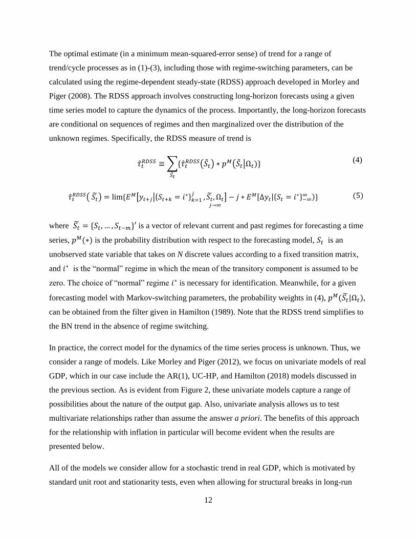

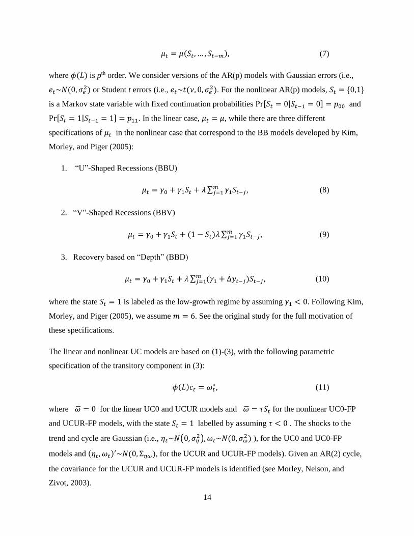
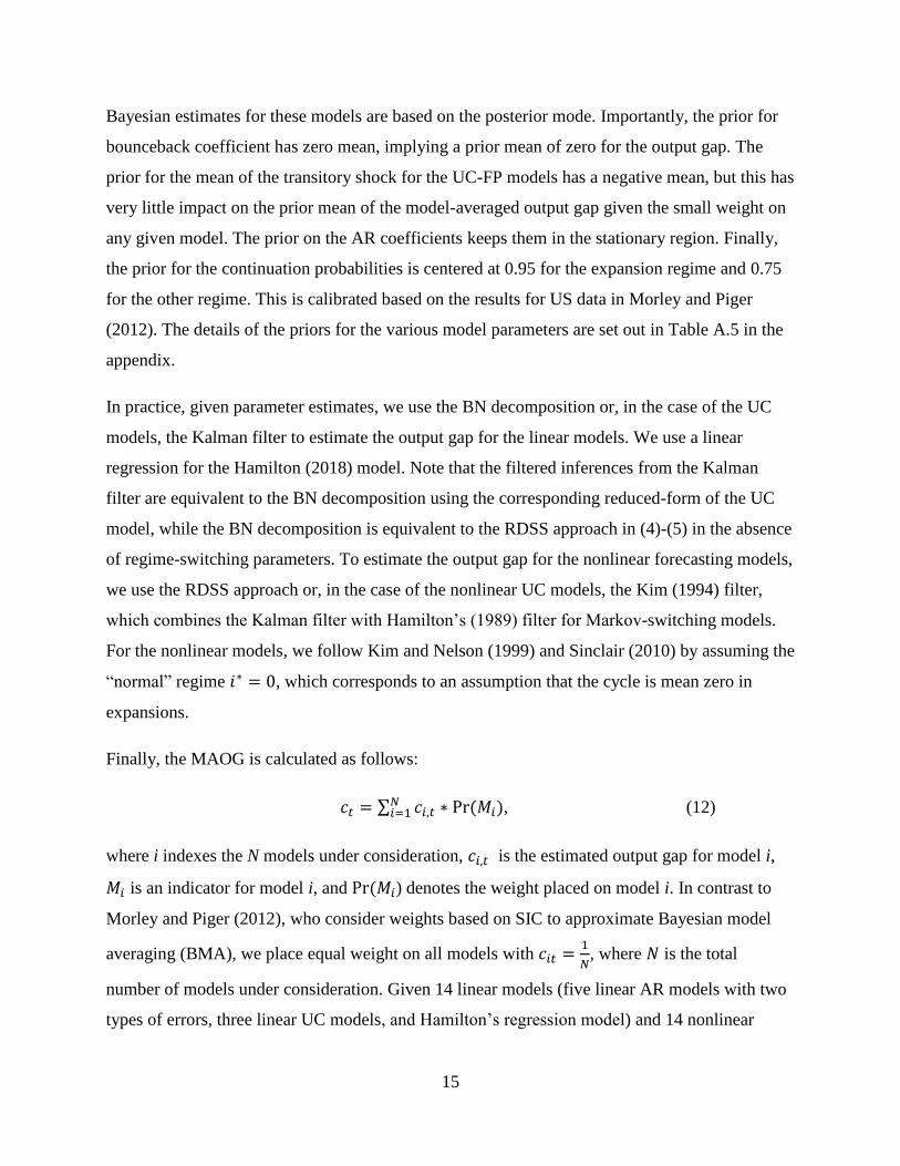


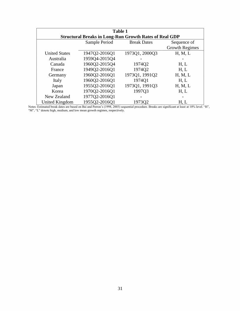
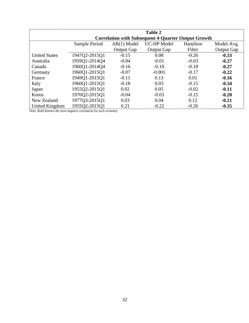


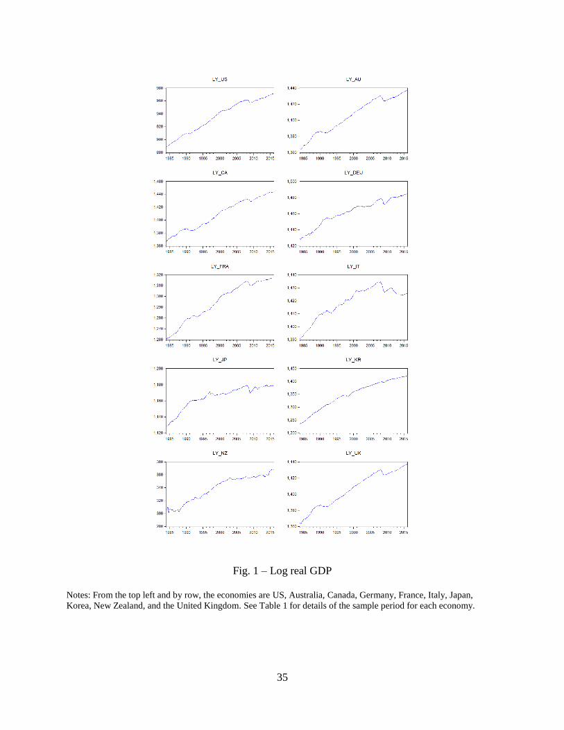
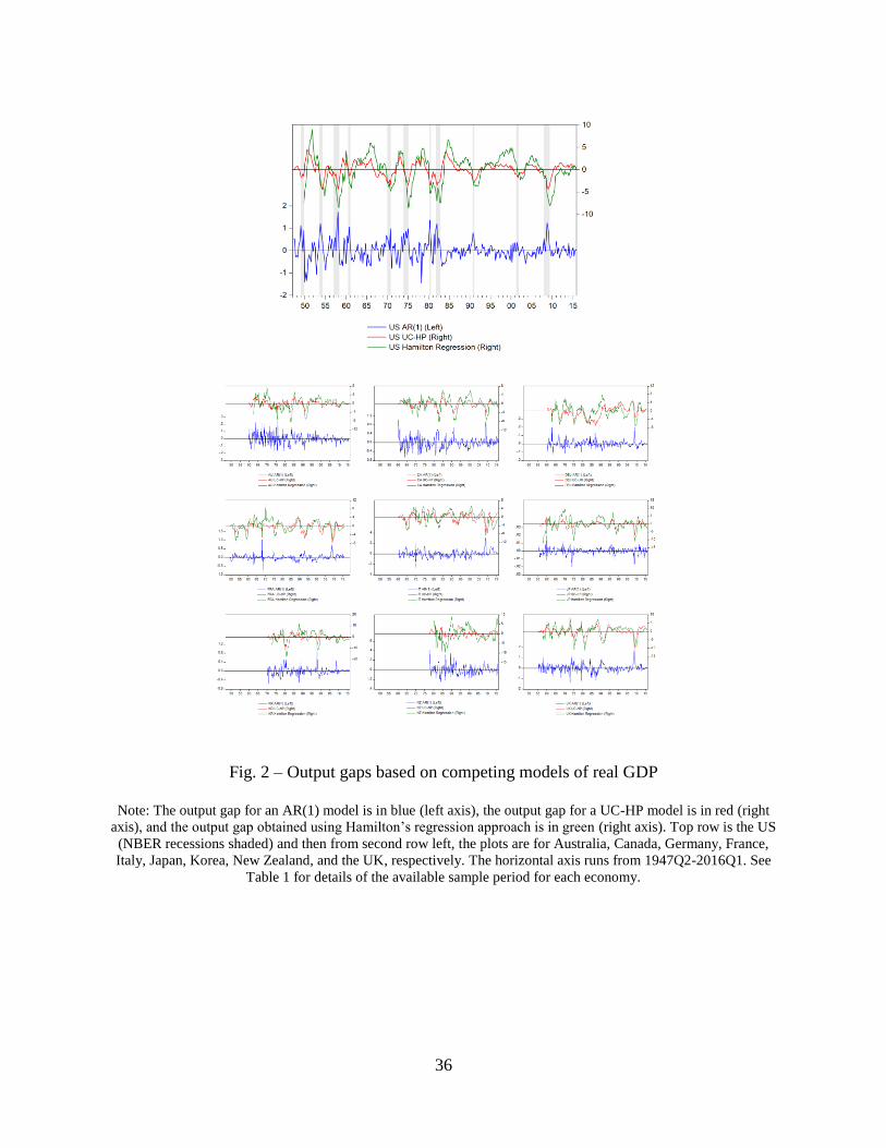
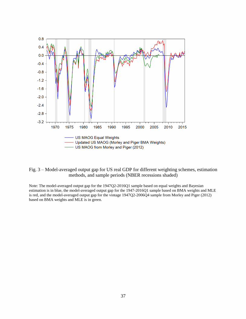

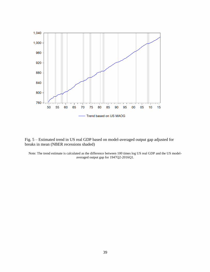
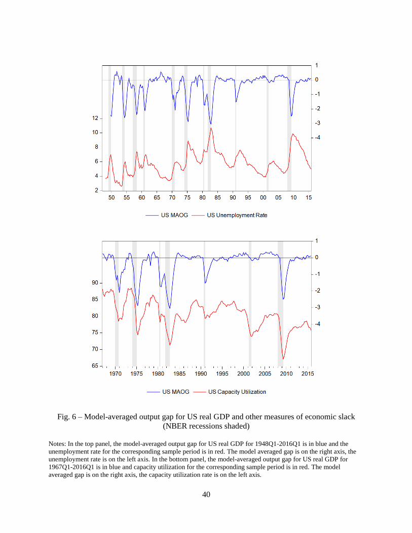

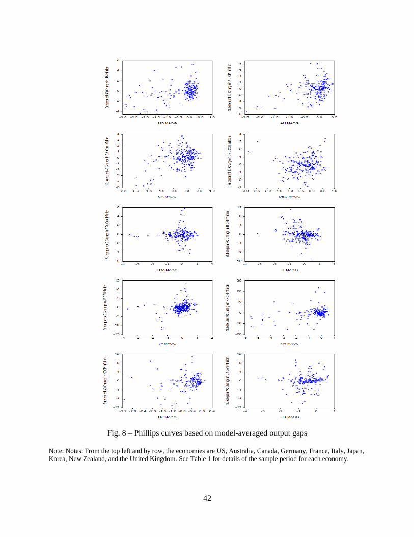
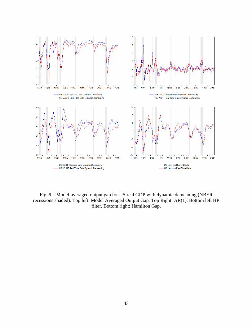


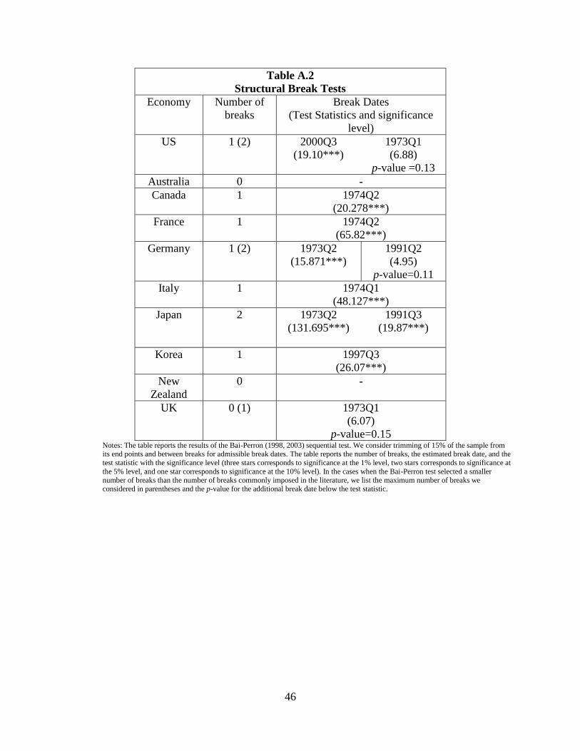

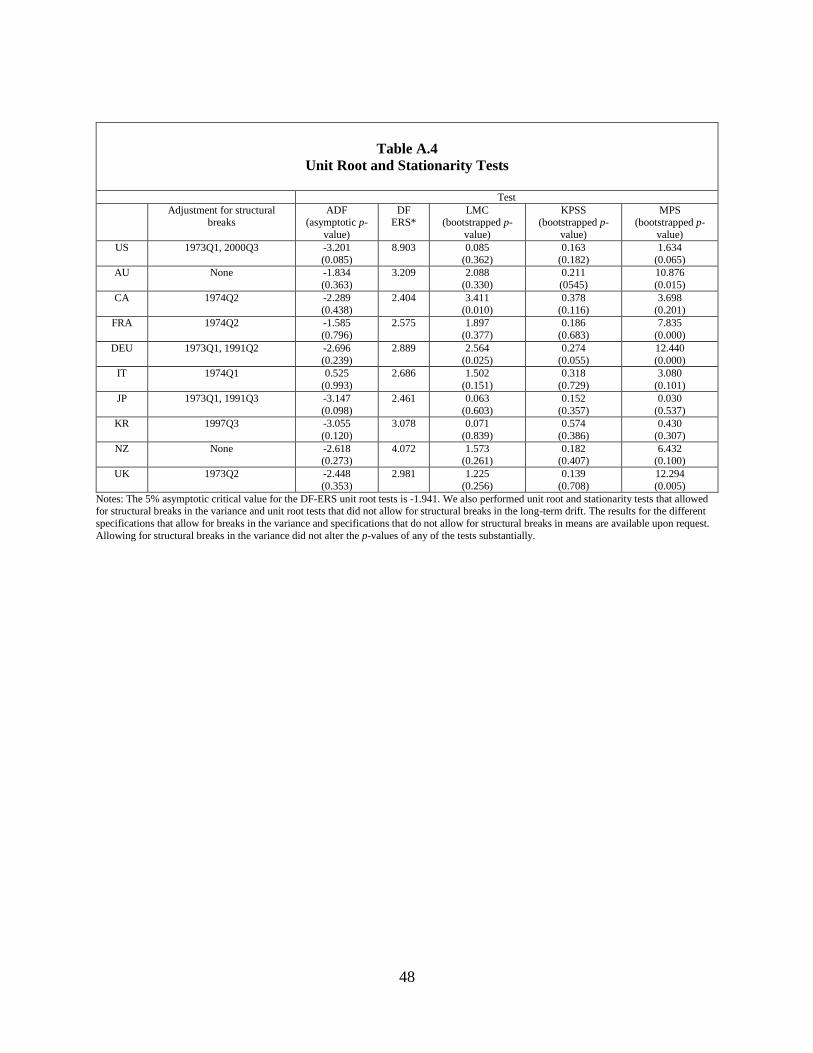


![Information Bottleneck Learning Using Privileged ... · testing, without considering the intrinsic asymmetry of the LUPIframework,aspointedoutin[42]. Theretheypropose two principles](https://static.documents.pub/doc/80x56/5fd49cc1680d7007c50d2599/information-bottleneck-learning-using-privileged-testing-without-considering.jpg)


