Is Inequality Harmful for Innovation

and Growth? Price versus Market Size

Effects

Reto Foellmi, University of St. Gallen and CEPR∗

Josef Zweimüller, University of Zurich and CEPR†

January 26, 2016

Abstract

We introduce non-homothetic preferences into an R&D based growth

model to study how demand forces hape the impact of inequality on

innovation and growth. Inequality affects the incentive to innovate via

a price effect and a market size effect. When innovators have a large

productivity advantage over traditional producers a higher extent of

inequality tends to increase innovators’prices and mark-ups. When

this productivity gap is small, however, a redistribution from the rich

to the poor increases market sizes and speeds up growth.

JEL classification: O15, O31, D30, D40, L16

Keywords: inequality, growth, demand composition, price distortion.

∗University of St. Gallen, Department of Economics - SIAW, Bodanstrasse 8, CH-9000

St.Gallen, Tel: +41 71 224 22 69, Fax: +41 71 224 22 98, email: reto.foellmi@unisg.ch†University of Zurich, Department of Economics, Schoenberggasse 1, CH-8001 Zürich,

Tel: +41-44-634-3724, Fax: +41-44-634-4907, e-mail: josef.zweimueller@econ.uzh.ch.

Josef Zweimüller is also associated with CESifo and IZA.

1

1 Introduction

The distribution of income and wealth across households may affect incen-

tives to undertake R&D investments through price- and market-size effects.

On the one hand, innovations are fostered if there are rich consumers willing

to pay high prices for new products. On the other hand, profitable innova-

tions require suffi ciently large markets, which may be lacking when income

are concentrated among a small number of rich households. Several previous

writers have mentioned the importance of price and market size effects for

innovation and growth. A prominent advocate for the importance of price

effects is von Hayek (1953) who argues that progressive taxation would be

detrimental for innovation incentives by reducing rich consumers’willingness

to pay for new goods. In contrast, Schmookler (1966) provides a forceful

statement emphasizing the relevance of market size effect in fostering R&D

investments.

To study these competing forces of income inequality, we introduce non-

homothetic preferences into a standard R&D based growth model. House-

holds either consume one unit of a particular product or do not consume

it. The assumption of such binary consumption implies that consumer get

quickly satiated within a product line. (By assumption, consuming more

than one unit of a product does not generate utility.) In such a framework,

demand can only keep pace with income growth when new products are

invented or when there are other (non-innovative) sectors that can absorb

the residual demand. We assume that goods are produced by monopolis-

tic firms who, after having made an innovation, have a monopoly on their

product. We also assume that there is a non-innovative sector (which could,

alternatively, be leisure or home production) that captures the residual de-

mand of rich consumers. Within this framework, we can characterize the

relative importance of price and market size effects which affect innovation

incentives in opposite directions. Higher inequality increases the demand

2

for non-innovative goods, because some rich consumers are already satiated

with innovative products, redistributing income towards them diverts de-

mand from the innovative to the non-innovative sector. This “market size”

effect reduces the incentive to innovate. However, higher inequality may also

raise the willingness to pay for innovative products for those beneficiaries are

not yet satiated with innovative products. The higher willingnesses to pay

allow innovators to increase the mark-ups. These “price” effects increase

the incentive to innovate.

Our paper builds upon mainstream endogenous growth literature. On

the consumption side, we assume that consumers are rational, forward look-

ing and have time-invariant preferences. They have the same preferences

which are unrelated to the economic role of the individuals. (This is differ-

ent from e.g. the Post-Keynesian literature where propensities to save and

consume differ by economic classes.) However, our approach differs from

standard models because we assume that preferences are non-homothetic.

This assumption implies that the distribution of income and wealth affects

the demand for innovative products. On the production side, we follow the

mainstream literature. Producers have fixed set-up costs and operate in an

environment of monopolistic competition. Restricting ourselves to a par-

simonious set of assumptions, we end up with a tractable framework that

has interesting implications for the relationship between inequality, innova-

tion and growth. In line with a large part of the mainstream literature our

analysis focuses on balanced growth paths. The advantage of this approach

is that the economic impact of changing an exogenous policy parameter can

be understood well by comparative statics. Clearly, the drawback is that

balanced growth analysis does not allow for feedback loops which are an

important feature of the evolutionary literature. We come back to this issue

in the discussion section.

A few previous papers have studied the role of income distribution on

3

incentives to innovate via price- and/or market-size effects. In Murphy et

al. (1989) a more egalitarian distribution increases the expenditure share for

innovative goods and reduces the share of traditional products thus foster-

ing industrialization. Their model emphasizes the market size effect, while

potential effects on prices are ruled out by the assumption of constant prices

and mark-ups. Moreover, their model is static and does not study the im-

pact of inequality on growth. Falkinger (1994) studies a model of growth

along a hierarchy of wants. He shows that the inequality growth relation

depends on the nature of the technical progress but his model does not con-

sider price effects. The present paper differs from our own previous work

because of its emphasis on the relative importance of price and market size

effects for the inequality-growth relationship. The analysis in Foellmi and

Zweimüller (2006) does not allow for market-size effects. In that framework

monopolistic producers do not face any restrictions in their pricing behavior

because of the absence of a sector absorbing the residual demand of satiated

rich consumers. This implies very high willingnesses to pay for new prod-

ucts and hence stronger innovation incentives when inequality increases. In

Foellmi, Wuergler and Zweimüller (2014) we elaborate the potential impact

of inequality on the introduction of high-quality luxury products versus low-

quality mass products. In that framework, the inequality growth relation-

ship depends on the nature of technical progress, i.e. whether new product

innovations or the introduction of mass production technologies drive tech-

nical progress. This is quite different from the present model where price

and market-size effects arise in a more parsimonious framework of horizontal

innovations (and without any quality differentiation).1

1Non-homothetic preferences have turned out important to explain the structural

changes in employment and output in long-run growth, see Matsuyama (1992, 2008),

Buera and Kaboski (2006), Foellmi and Zweimüller (2008), and Boppart (2014). Other

papers have studied how inequality affects growth via non-homotheticities have also em-

phasized market size effects. In Matsuyama (2002) technical progress is driven by learning

4

There is an established heterodox literature that studies the interrela-

tionship between consumption/savings, inequality and growth. We come

back to seminal contribution of Kaldor (1966) in the discussion section. For

recent contributions in the Post-Keynesian tradition, see Salvadori (2006),

Kurz and Salvadori (2010), and Araujo (2013). An important issue in the

evolutionary literature is the question how consumer wants emerge and gen-

erate suffi cient demand in an environment of growing incomes (Witt, 2001).

The problem of demand growth is crucial in our framework, where con-

sumers are quickly satiated with existing products and demand can only

keep pace with growing incomes when new goods are introduced.2 Several

recent studies explore agent-based frameworks to understand the relation

(and feedback loops) of growth, inequality and consumption patterns. Cia-

rli et al. (2010) study an agent-based framework where technological changes

lead to changes in the income distribution that feed back to consumption

patterns. Bernardino and Araujo (2013) explore the importance of inequal-

ity when technical progress is driven by the demand for positional goods.

Lorentz et al. (2015) study how the micro-dynamics of consumption behav-

ior are related to inequality and they show that increased heterogeneity in

consumer’s reaction to income changes affect firm selection and the dynamics

by doing and an intermediate degree of inequality is required to realize the full learning

potential. Falkinger (1994) studies the impact on inequality on market sizes under the

assumption of exogenously given profit-margins. In Chou and Talmain (1996) consumers

have non-homothetic preferences over a homogenous consumption good and a (CES) bun-

dle of differentiated goods which affects the market size (but not the mark-up) of in-

novators. Zweimüller (2000) provides a dynamic version of Murphy et al. (1989). In

Galor and Moav (2004) non-homotheticities affect growth via savings rates that differ by

income. A very different strand of the literature studies the interrelationship between

consumption/savings, inequality and growth in the Post-Keynesian tradition. For recent

contributions, see Salvadori (2006) and Kurz and Salvadori (2010).2Empirical evidence suggests that the diversity of consumption is closely linked to

household income, see e.g. Jackson (1984), Falkinger and Zweimüller (1996), Chai and

Rohde (2012).

5

of market structure.

Our analysis provides a theoretical framework for a better understand-

ing of the role of demand forces in the inequality growth relationship. The

initial empirical literature provided support for the idea that inequality is

harmful for growth (Alesina and Rodrik, 1994, Persson and Tabellini 1994,

Deininger and Squire 1996), while more recent studies do not support such

a clear-cut relationship. Barro (2000, 2008) shows that there is a positive

relationship for rich countries but a negative one for poor countries. Forbes

(2000), using panel data, finds a positive relationship. The more recent lit-

erature uses new and better data and also tries to overcome methodological

shortcomings of previous studies. However, the new studies were not able to

come up with clear-cut results. Banerjee and Duflo (2003) find nonlinear re-

lationships between inequality and growth, while Voitchovsky (2005) shows

that inequality at the top is positively and inequality at the bottom is neg-

atively related to subsequent growth. More recent work by Berg and Ostry

(2011) find that more equal counties have significantly longer growth spells.

Halter et al. (2014) argue that inequality may affect growth negatively in

the short run, but positively in the long run. Ostry et al. (2015) point to the

important distinction of the effects on growth of pre-tax inequality and of

redistribution through the tax transfer-system. However, the new empirical

studies were not able to come up with clear-cut results (see Voitchovsky 2009

and Boushey and Price 2014 for recent surveys). It is therefore important

to understand the mechanisms through which ambiguities may arise.

In Section 2 we present the main assumptions of the model. Section 3

discusses price determination and market sizes and their implications for

the incentives to undertake R&D investments. In Section 4 we look at the

balanced growth path. Section 5 studies the impact of inequality on long-

run growth and Section 6 provides a discussion of important assumptions

and how they affect the inequality-growth relationship.

6

2 The model

Endowments and distribution. Consider an economy with a unit mea-

sure of households whose aggregate supply of labor is L, constant over time.

Households get income from wages and profits. At date t there are N(t)

monopolistic firms generating positive profits. There is a nondegenerate dis-

tribution of income reflecting both skill differences and differences in capital

ownership. A household is endowed with θ units of labor and θN(t) shares

of profitable firms, where θ is distributed across households with the cdf

G(θ) with support[θ, θ]. A household with endowment θ earns labor in-

come θw(t)L and capital income θr(t)V (t) where w(t) is the wage rate per

unit of effective labor, r(t) is the interest rate, and V (t) is the aggregate

value of assets (i.e. the capitalized value of all existing firms). The resulting

distribution is shown in the Lorenz curve of Figure 1 below.3

Figure 1

Preferences and consumption choices. All households have the same

preferences. There is an infinitely large number of potentially producible

goods, j ∈ [0,∞). All goods are equally valued by the household. Goods

are consumed in discrete amounts and the household is saturated after con-

suming one unit. We denote by x(j, t) the indicator function such that

x(j, t) = 1 if good j is consumed at date t, and x(j, t) = 0 if not.

Households have an infinite horizon. A household with endowment θ

chooses {x(θ, j, t)}j=∞,t=∞j=0,t=τ to maximize∫ ∞τ

log

[∫ ∞0

x(θ, j, t)dj

]e−ρ(t−τ)dt

3The assumption that labor and capital endowments are perfectly correlated and iden-

tically distributed is made for analytical convenience. Below we assume additive and loga-

rithmic intertemporal preferences generating equal optimal savings rates for all households.

This assumption (and the absence of income shocks) ensures that the initial distribution

of θ persists over time. Hence time indices for θ are omitted.

7

subject to∫ ∞τ

[∫ ∞0

p(j, t)x(θ, j, t)dj

]e−R(t,τ)dt ≤ θ

[∫ ∞τ

w(t)Le−R(t,τ)dt+ V (τ)

]where p(j, t) is the price of good j at date t, and R(t, τ) =

∫ tτ r(s)ds is

the cumulative interest factor.4 The optimal solution to this intertemporal

choice problem satisfies the first-order condition

x(θ, j, t) =

1, p(j, t) ≤ z(θ, t)

0, p(j, t) > z(θ, t)

where z(θ, t) ≡ eR(τ ,t)−ρ(t−τ)

µ(θ)N(θ, t), (1)

where z(θ, t) is the household’s willingness to pay. Here z(θ, t) is inversely

related to µ(θ), the household’s time-0 marginal value of wealth (the La-

grangian multiplier), and to N(θ, t) ≡[∫∞

0 x(θ, j, t)dj], the optimal quantity

consumed at date t. Equation (1) represents a simple consumption rule: A

household with endowment θ purchases good j at date t if the price of this

good, p(j, t), does not exceed the consumer’s willingness to pay at that date.

Consequently, individual demand is a simple step function, see Figure 2.

Figure 2

Production and technical progress. The supply side of the model is

very simple. All goods are produced with identical technologies and labor

is the only production factor. Each good can be produced in two different

ways, with a traditional and innovative technology. The traditional backstop

technology has productivity β(t) and operates under constant returns to

scale. and the innovative technology has productivity α(t) with β(t) < α(t).

Unlike the traditional technology (that produces under constant returns to

scale), the innovative technology requires an initial (one-time) set-up effort

equal to Φ(t) units of labor. A firm that incurs this set-up cost makes an

4The log intertemporal utility is used for ease of exposition. The same results would

hold true (in particular the invariance of distribution) if the utility would be CRRA in

the consumption aggregator∫∞0x(θ, j, t)dj.

8

“innovation”. Think of an innovation as a completely new good that crowds

out traditional products or, alternatively, as an improved way to produce an

already existing good.5 (Both interpretations are valid as both existing and

new goods enter the utility function symmetrically). In line with endogenous

growth theories, we assume that the knowledge stock of this economy equals

the number of innovations that have taken place up to date t, denoted by

N(t). It is assumed that Φ(t) = F/N(t), α(t) = aN(t) and β(t) = bN(t)

where F > 0 and a > b > 0 are exogenous parameters. We normalize labor

costs in the traditional sector to unity w(t)/β(t) = 1. Under our assumption

on the knowledge stock, this implies that the growth rate of wages equals

the rate of innovation, w(t) = bN(t). This implies that production costs in

the innovative sector are w(t)/α(t) = b/a < 1, and the innovation cost are

w(t)Φ(t) = bF , constant over time.

3 Prices, market sizes, and innovation incentives

Price setting of monopolistic firms. There is a measure of N(t) mo-

nopolistic firms, equal to the number of innovations, on the market. By

symmetry, all firms face the same cost- and demand-curves. The represen-

tative firm faces a trade-off between setting a high price and selling to a

small group of consumers (and vice versa). The traditional technology is

freely accessible, hence the innovative firm has to choose a price lower than

(or equal to) unity to prevent the competitive fringe from entering the mar-

ket. Consumers purchase the goods with the lowest prices until they exhaust

their budget.

The equilibrium outcome is most easy to grasp when there are only two

groups, rich and poor. The representative firm faces the choice between

5An isomorphic case would the situation where innovative firms produce a better prod-

uct, yielding higher utility, with the same production technology as traditional firms (or

some combination of productivity/quality gain).

9

selling only to the rich at a high price; or selling to all households at a

price low price. For obvious reasons, a situation where all firms sell to all

consumers or where all firms sell only to the rich can not be an equilibrium.

In the former case, both groups would have identical expenditures and in the

latter case, the poor would have no expenditures implying that one of the

two groups does not exhaust its budget. As left-over budgets are associated

with very high willingnesses to pay for the marginal good, firms have an

incentive to deviate in both cases. In equilibrium, an (endogenous) fraction

of firms sells exclusively to the rich and the remaining fraction of firms sells

to all households. The former set a price that equals the willingness to pay

of the rich and the latter set a price that equals the willingness to pay of

the poor. In equilibrium, both types of firms make the same profit and

both types of households exhaust their budget. Obviously, these arguments

generalize to K > 2 discrete groups.6

A continuous distribution G(θ) generates a continuous distribution of

prices and firm sizes. We label of a firm as type θ when it sells to all

households with endowment θ or richer (and has market size [1 − G(θ)]L).

A firm of type θ charges a price p(θ) = z(θ), the willingness to pay of

household θ.7 Notice that p(θ) is increasing in θ, reflecting the basic trade-

off that firms face: either they sell at low prices and high quantity (the

market size [1 − G(θ)]L is decreasing in θ) or they set higher prices but

have a smaller market size. Due to the competitive fringe, modern firms are

6With K groups of consumers, there are K firm types such that type 1 sells to the

richest group (and charges their willingness to pay), the second type sells to the richest

and second richest (and charges the willingness to pay of the second richtest group), ....,

and the Kth type sells to all households (charging the willingness to pay of the poorest

group). In equilibrium the distribution of firms across types is endogenous and satisfies

conditions (i) and (ii) mentioned in text.7 Instead of writing consumption expenditures of a household with endowment θ as∫ N(θ)

0p(j)dj we can write

∫ θθp(θ)dN(θ) + p(θ)N(θ) where N(θ) and p(θ) are the menu

and the price of the goods that the poorest household can afford.

10

limited to types θ ∈ [θ, θ] where firm θ charges a price p(θ) = 1 and has

profits [1−G(θ)]L[1− b/a] = π.

The equilibrium firm size distribution is given as follows: A measure

n(θ) of monopolistic firms sells to all consumers and produces L units. The

firm size distribution is continuous and determined by the endowment dis-

tribution G(θ) (see Lemma 1 below). Each firm makes the same profit

π = [1−G(θ)]L [p(θ)− b/a] for all θ ∈ [θ, θ]. Consumers with θ < θ con-

sume only a subset of innovative goods and consumers with θ > θ consume

all innovative goods and some traditional products supplied by the compet-

itive fringe. Our analysis below treats θ as the crucial endogenous variable

(in addition to the endogenously determined growth rate).

Zero profit condition. The costs of an innovation are bF , constant over

time (see above). The value of an innovation equals the profit flow associated

with a monopoly position. We assume an innovator gets a patent that lasts

forever. The profit flow is equal to π = [1 − G(θ)]L[1 − b/a], independent

of t as long as θ is time-invariant which is the case along a balanced growth

path. Along this path the interest rate is constant, r(t) = r, and the value

of the innovation is given by∫∞t π exp(−r (s− t))dt = π/r. In equilibrium,

the value of an innovation may not exceed innovation costs, π/r ≤ bF. This

condition holds with equality when innovation takes place. The zero-profit

condition can then be written as

rbF = [1−G(θ)]L[1− b/a]. (2)

4 The balanced growth path

Along the balanced growth path, the economy’s resources are fully uti-

lized. Labor demand in research is N(t)Φ(t). Using Φ(t) = F/N(t) and

the definition g ≡ N(t)/N(t) we get N(t)Φ(t) = gF . Labor demand in

production comes either from innovative monopolistic producers or from

11

traditional competitive producers. A consumer with endowment θ ≤ θ

purchases N(θ, t) goods supplied by innovative producers which requires

N(θ, t)/α(t) = [N(θ, t)/N(t)] /a units of labor. A consumer with endow-

ment θ > θ purchases all N(t) goods by innovative producers and N(θ, t)−

N(t) goods by traditional producers which requires [N(θ, t)−N(t)] /β(t) +

N(t)/α(t) = 1/a + [N(θ, t)/N(t)− 1] /b units of labor. In a steady state,

where the distribution of income and wealth is stationary, consumption

N(θ, t) grows at the same constant rate g for all consumers. Defining

n(θ) ≡ N(θ, t)/N(t), we see that n(θ)/a units of labor are needed to pro-

duce the goods consumed by household θ ≤ θ; and 1/a + (n(θ) − 1)/b for

household θ > θ. Summing up labor demands and setting them equal to

aggregate labor supply yields the full employment condition

L = gF +L

a

(∫ θ

θn(θ)dG(θ) + 1−G(θ)

)+L

b

∫ θ

θ(n(θ)− 1) dG(θ).

Lemma 1 Along the balanced growth path a) the stationary distribution

of endowments G(θ) is associated with stationary prices p(θ); consumption

expenditures equal to N(t)θb [1 + ρF/L] and consumption growth g = r− ρ;

b) the optimal consumption levels are:

n(θ) =

aθ L+ρF

(g+ρ)aF+L θ = θ

a∫ θ

0(L+ρF )(1−G(ξ))

(g+ρ)aF+L(1−G(ξ))dξ θ < θ < θ

1 + (L+ ρF ) (θ − θ)b/L θ ≥ θ

(3)

Proof. See Appendix.

In steady state, consumers with relative wealth θ consume all innovative

goods, hence n(θ) = 1 or

1 = a

∫ θ

0

(L+ ρF ) (1−G(θ))

(g + ρ)aF + L (1−G(θ))dθ. (4)

12

The resulting consumption structure of innovative goods is depicted in Fig-

ure 3. The poorest consumers buy only a fraction n(θ) of the innovative

products, while households with wealth θ > θ buy all innovative products.

Figure 3

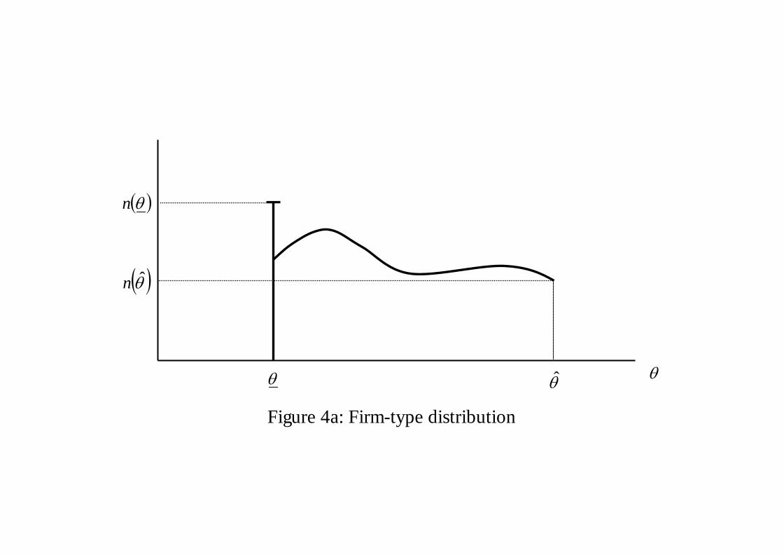
This gives rise to a firm type and size distribution (Figure 4). Denote the

poorest consumer served by a distinct firm as critical consumer. There is a

continuum of firm where the critical consumers have wealth θ > θ, instead a

positive mass firms sell to all consumers. Correspondingly, there is a positive

mass of firms with size L (Figure 4b.).

Figure 4a. and b.

The general equilibrium of the model is characterized by the two equa-

tions (2) and (4) in the two unknowns g and θ. Note that resource constraint

holds when both (2) and (4) simultaneously are satisfied. We analyze the

equilibrium graphically (Figure 3).

Figure 5

The zero profit condition is a decreasing curve in the (g, θ)-space. If θ

increases, market size is smaller (recall that p(θ) = 1 which is constant),

hence the real interest rate r = ρ+g must be smaller such as to guarantee a

zero profit equilibrium. The consumption equation (4) is an increasing curve

in the (g, θ)-space. In general equilibrium, higher growth rates must go hand

in hand with larger prices and therefore lower expenditures. Therefore, the

relative wealth θ must be larger such that n(θ) = 1 holds.

13

5 The impact of inequality on growth

We concentrate on the relevant case where only suffi ciently rich consumers

are able to purchase all modern products. Such an equilibrium emerges

when θ (1 + ρF/L) < 1/b. To see this, notice that an equilibrium with θ > θ

(such that some households cannot afford to buy all goods) requires that,

at θ = θ, the value of g that satisfies the zero profit constraint (2) has to

exceed the value of g in the consumption equation (4). If this condition is

violated even the poorest consumer buys all innovative products. In such

an equilibrium, the prices of all innovative goods are unity (all monopolistic

firms have to charge a price that deters entry from competitive producers)

and market size is at its highest possible level. In such an equilibrium,

changes in inequality do not have an impact on growth.

Assuming θ (1 + ρF/L) < 1/b, we are now ready to analyze the effect of

more inequality.

Proposition 1 a. A regressive transfer among consumers with θ < θ

increases the growth rate. b. A regressive transfer from a consumer with

θ < θ to a consumer with θ > θ reduces the growth rate. c. A regressive

transfer among consumers with θ > θ leaves the growth rate unaffected.

Proof See Appendix.

The reason behind part a. of the above proposition is the dominance

of the price effect. A regressive transfer among consumers with θ < θ is

a transfer from consumers who pay a lower average mark-up to consumers

who pay on average a higher mark-up. Therefore a regressive transfer among

consumers with θ < θ increases average prices and mark-ups. In the new

equilibrium the profit flow π of innovative producers is larger which increases

the incentive for further innovation. Figure 6a. characterizes part a. of the

proposition graphically.

14

Part b. of the proposition reflects the dominance of the market size

effect. A regressive transfer from a consumer with θ0 < θ to a consumer

with θ1 > θ implies an decrease in demand for monopolistic producers and

an increase in demand for traditional producers. In particular, household

θ0 has a lower willingness to pay and hence firm θ0 experiences a fall in its

price. In equilibrium all firms earn the same profit. Hence the reduction

in the price for one firm must decrease the prices for other firms. The

result is a reduced incentive to innovate. Figure 6b. shows the change in

the equilibrium curves for a regressive transfer from the consumer of the

“middle class”with θ0 < θ to a rich consumer with θ1 > θ.

Finally, part c. of the proposition results from the fact that a redistribu-

tion among households with θ > θ does not affect the demand for innovative

products at all and leave prices and market size of innovative firms unaf-

fected.

Figure 6a. and b.

How do our results relate to existing demand explanations of the relation-

ship between inequality and growth? It is crucial for the inequality-growth

relationship to which innovative firms are constrained in their price setting

behavior. In the polar case where no competitive fringe exists (as in Foellmi

and Zweimüller, 2006), only price effects are at work and inequality is ben-

eficial for growth. In the presence of a competitive fringe, it is the cost

advantage of innovators that determines the scope for price setting. If the

technology gap is small, price effects are weak and market size effects domi-

nate implying that inequality is harmful for growth. Our model encompasses

both mechanisms. When the productivity gap between the innovative sector

and the traditional sector a/b > 1 is very high, θ approaches θ. In that case,

only the very rich can afford all innovative products, all households (except

the richest) consume only a subset of innovative goods, and the competi-

15

tive fringe has only a tiny market share. Consequently, regressive transfers

increase growth.

Foellmi, Wuergler, and Zweimüller (2014) allow for quality differentia-

tion to generate market size effects. Innovators supply high-quality products

to the rich and mass products to the poor. In a highly unequal economy,

most firms supply only high-quality to serve rich consumers while in an egal-

itarian society, mass production is more prevalent. The extent of inequality

determines the relative attractiveness of introducing new products versus

implementing mass production of existing products. Whether inequality

is beneficial or harmful for growth depends on the nature of technology:

When the introduction of mass production technology is the driver of tech-

nical progress, high inequality decreases growth. The opposite is true when

the product innovations (i.e. the invention of high-quality goods for the

rich) are the engine of growth. In contrast to Wuergler et al. (2014), the

present paper generates price- and market size effects even in the absence

of quality differentiation.

Our model also encompasses the situation studied in Murphy et al.

(1989). Similar to their model, a regressive transfer from households who

cannot purchase all innovative goods to consumers who can afford all these

goods, decreases innovators’market size and depresses growth. However, in

Murphy et al. (1989) only the market size effect is at work and price effects

are ruled out by assumption. Hence a redistribution among consumers θ < θ

(all of whom cannot purchase the entire menu of innovative goods) leaves

the the number of industrializing sectors unaffected in their model as the

market size effect is at work only. In contrast, in our analysis such a redistri-

bution generates price effects that lead to a positive impact of inequality on

growth. In sum, our model predicts that redistributions towards consumers

just below θ, both from below and from above, increases in growth.

As changes in inequality affect the growth rate, it is interesting to ask

16

whether growth-increasing redistributions can lead to Pareto-improving out-

comes. Interestingly, the answer is a qualified yes for both types of redistri-

butions. The group of donating households loses on impact but gains from

a steeper consumption path in the long run. Pareto-improvements may oc-

cur if the rate of time preference is very low, so that the donators values

dynamic gains more strongly than static losses. Pareto-improvements are

also more likely the higher the standard of living of the donators. In that

case, static losses are smaller (due to lower marginal utilities).

6 Discussion

The above relationship between inequality and growth has focused on a bal-

anced growth path derived under simplifying (and restrictive) assumptions

on the distribution of wages and profits. The purpose of this section is

to discuss the robustness of our results and their relations to the related

evolutionary and Post-Keynesian literature. In particular, we discuss what

happens when we allow for (i) asymmetric distributions of labor earnings and

capital incomes and (ii) non-stationarities and feedback effects from growth

to inequality. The main message is that adding realism to our distributional

assumptions makes the model much more complex but does not change the

results qualitatively. Moreover our model is also a useful starting point for

more general non-stationary environments. In this sense, the assumptions

are made for simplicity, but carry over to more general situations.

Endogeneity of the income distribution. The first point we want to

emphasize is that the stationarity of the income distribution is not an as-

sumption about exogenous parameters, but an endogenous outcome of the

model. A household has labor endowment θL(t)L and wealth endowment

θΠ(t)V (t) and the particular assumption we made to solve the model was

that θL(t)L(t) = θL and θΠ(τ)V (τ) = θV (τ) where τ is the initial period

17

when the economy starts. Only the distribution of labor endowments is

truly exogenous (and time-invariant) implying that households’ labor in-

comes w(t)θL grow pari passu with the competitive wage w(t) and its dis-

tribution stays constant by assumption. However, the assumption on the

wealth distribution refers only to initial wealth endowments (i.e. the dis-

tribution of V (t) at the initial date τ). To keep the analysis simple, we

assumed that the initial wealth endowment distribution coincides with the

labor endowment distribution, so that θΠ(τ) = θL(τ) = θ. Notice also that

θΠ(t) = θ in later periods t > τ is an endogenous outcome, resulting from

optimal savings choices. The stationarity result θΠ(t) = θ hinges on the

assumption of intertemporal CRRA preferences. This assumption implies

that, in steady-state, all households save at the same rate from capital in-

come, implying that individual wealth levels of rich and poor consumers

grow pari passu (see Bertola et al. 2006). We discuss below that deviating

from CRRA generates non-stationarities and feedback effects from growth

to inequality.

Asymmetric labor- and wealth-endowment distributions. The as-

sumption that labor earnings and wealth are symmetrically distributed is

clearly very stylized and not realistic from an empirical point of view. In

empirical data there is no perfect correlation between labor earnings and

capital incomes in a cross section of households (although the correlation is

positive: high-wage households tend to also have higher wealth than low-

wage households). More importantly, wealth and capital incomes are much

more unequally distributed than labor incomes. It is therefore important to

ask: Does the result of Proposition 1 hinge upon symmetry of the earnings

and wealth distributions?

It turns out that the answer is “no”. The symmetry assumption is a sim-

plifying assumption and deviating from this assumption does not generate

18

substantive new insights. An increase in income inequality (from whatever

source) will affect (i) the distribution of households’willingness to pay for

innovative products and (ii) the composition of demand for innovative ver-

sus backstop products. Asymmetric income sources complicate the analysis

since (i) we need to specify how a change in inequality of a particular income

source translates into a more unequal distribution of income before we can

discuss (ii) the impact on growth. In the symmetric case, step (i) is trivial

and allows us to move to step (ii) immediately; in the asymmetric case step

(i) is more complicated to solve —although is can be done and we briefly

sketch here how this changes proposition 1.

With symmetry, step (i) is trivial because there is one critical relative

endowment, θ, leading to the critical willingness to pay, z, at which the

household purchases all innovative products but no backstop goods. With

asymmetric labor and wealth distributions, z depends on the mix of (θL, θΠ)

and there are, in general, many different combinations of (θL, θΠ) that lead

to the same z. However, once we have determined z, the impact on inequality

on growth along the lines of proposition 1: When a change in the distribution

of income source j = (L, V (τ)) translates into an regressive income transfer

among consumers with z(θL, θH) < z innovation and growth increases. A

change in the distribution of incomes source j that translates into a regressive

transfer from a consumer with z(θL, θH) < z to a consumer with z(θL, θH) >

z decreases growth. Finally, when the change in the distribution is associated

with a regressive transfer among consumers with z(θL, θH) > z innovative

activity and growth are unaffected.

Nonstationarities, feedback effects and relation to the heterodox

literature. Both the evolutionary and Post-Keynesian literature have em-

phasized that scale economies and increasing returns are central to under-

stand economic growth. This argument, dating back at least to Young

19

(1928), or even to Adam Smith’s pin factory, has been taken up by the

mainstream endogenous growth literature as well. In the Post-Keynesian

tradition, Kaldor (1966, 1981) developed the principle of cumulative cau-

sation, again building on earlier contributions by Veblen and Myrdal (see

Berger and Elsner, 2007). Kaldor argues that the structure of demand is

affected by the distribution of income and wealth across households and the

social structure. An expansion of demand sets a process of productivity

gains in motion: A larger market size allows for learning-by-doing and man-

ufacturers can increase vertical specialization. The implied reduction in the

cost of production implies a reduction in prices. This lets the product market

expand further, generating a virtuous cycle. This argument is central for the

structuralist school as well. Cumulative causation is important also in our

setting, albeit in a reduced form. The wealth distribution affects aggregate

demand which in turn determines innovation activities and productivity in-

creases through spillover effects. Because of symmetry, however, our model

is silent about different markets and the productivity-growth potential of

e.g. manufacturing versus services. In our extension discussed above, the

functional distribution between labor incomes and profits affect outcomes,

but through a different mechanism than put forward by the Post-Keynesian

literature.

The evolutionary literature addresses similar topics, in particular the

importance of demand growth and market scope for innovative products, as

well as the importance of scale economies through cumulative causation, see

e.g. Argyrous (1996). By assuming non-homothetic preferences and market

power, our analysis allows for structural change as well (e.g. Saviotti, 2001).

This is a further element that our analysis shares with the evolutionary liter-

ature. In our approach, structural change is captured in a simple way as all

adjustment occurs in the intensive margin. 8 The most important difference

8 In a model with representative agents, we analysed the extensive margin to study

20

from the evolutionary economics is that our analysis focuses on the balanced

growth path. Evolutionary economics understands growth essentially as a

disequilibrium process where Darwinian selection, e.g. on a firm level, plays

an important role with an emphasis of out-of-equilibrium dynamics due to

feedback loops.

Our analysis focuses on the balanced growth path. As mentioned in the

introduction, this allows for comparative static analysis that is relatively

easy to perform and understand. Clearly<, reality is far from such a “golden

age”, and feedback effects from growth to inequality are potentially very

important. In fact, an important literature started by Kuznets (1955) argues

that income inequality increases at low levels of development (in a transition

process from the traditional to the modern sector) and then decreases again

at later stages of development (when the economy is increasingly dominated

by the modern sector). This lead to the famous “Kuznets-curve”, a hump-

shaped feedback relation from growth to inequality. Notice however, that

empirical evidence does not support Kuznets’predictions. While inequality

has been decreasing during most of the 20th century —consistent with the

Kuznets hypothesis — it has been on the rise in many countries since the

late 1970s and a large literature discusses causes and possible cures (for

influential recent contributions see Piketty 2014 and Atkinson 2015).

It is therefore suggestive to ask how accounting for feedback effects from

growth to inequality qualifies the predictions of our analysis. It turns out

that feedback effects can be captured within our theoretical framework. The

important assumption generating a balanced growth path is the assumption

of intertemporal CRRA preferences. As mentioned above, this assump-

tion generates a situation where all labor incomes are consumed and where

there is a constant (time-invariant) optimal savings rate from capital in-

come. However, if preferences are not CRRA, this does not longer hold and

demand-driven structural change (Foellmi and Zweimueller, 2008).

21

there feedback effects from growth to inequality through systematic changes

in individual savings rates. As shown in Bertola et al. (2006), chap. 3,

preferences that feature decreasing relative risk aversion generate the em-

pirically relevant situation where the savings rate increases with income.

This implies that inequality increases with economic growth.9 What are the

consequences of such feedback effects for the inequality-growth relationship

studied here? Our model still provides predictions how inequality affects

growth even in such a non-stationary environment. In contrast to growth

along a balanced growth path, the above feedback effects imply that the

distribution of households’willingnesses to pay is become more unequal as

overall inequality increases. Increases in inequality among households who

cannot afford all innovative products will generate price effects, i.e. rising

mark-ups in the innovative sector increasing the incentive to innovate. On

the other hand, increases in inequality will also divert demand from the

innovative to the backstop sector (or, more generally, to sectors that do

not contribute to technical progress) and this market-size effect reduces the

impact of inequality on growth. Whether growth increases or decreases de-

pends on the relative importance of these price- and market size effects and

the relative important of these effects may vary over time.

Feedback effects from growth to inequality may not only occur through

savings. It may also be that, as the economy develops, poorer individuals

get better access to economic resources, they may become able to invest

(more) in human capital, get better access to capital markets and invest-

ment opportunities etc. These mechanisms generate feedback effects that

can reduce rather than increase inequality, generating less dispersed willing-

9The reference to “risk”is misleading here since risk and uncertainty do not play a role

in our analysis. CRRA features a constant elasticity of marginal utility with respect to

the level of consumption. In the present context, decreasing relative risk aversion (DRRA)

means that the elasticity of marginal utility is increasing with consumption, implying that

rich households save a larger fraction of their income that the poor.

22

nesses to pay and lower relative demand for the backstop sectors. Again,

such feedback mechanisms may generate non-stationarities and lead to con-

tinuous changes in willingnesses to pay and demand compositions over time.

However, innovation incentives will then be driven by the evolution of the

willingness to pay and market sizes. We conclude that the above analysis,

despite its focus on a balanced growth path, provides a useful framework also

for non-stationary environments. Price and market size effects affect inno-

vation and growth in qualitatively similar ways when the economy operates

off the balanced growth path.

Our analysis has focused on a closed economy. An important direction

for future research is to bring the international perspective into the picture.

Technological changes and globalization lead to increased inequalities within

countries but it also allowed low-income countries to grow, leading to a more

even distribution of incomes across countries. As markets become increas-

ingly global, the role of these inequality changes will generate important

price and market size effects on innovations on world markets.

23

Appendix

Proof of Lemma 1

Proof. a. Differentiating z(θ, t) with respect to t, using N(θ, t)/N(θ, t) = g,

yields z(θ, t)/z(θ, t) = r − ρ − g. Guess that g = r − ρ, so z(θ) is station-

ary. In that case household θ purchases all goods with prices lower than or

equal p(θ) at all times and pays average price p(θ), constant over time, and

has expenditures p(θ)N(θ, t). Notice further that wages evolve according to

w(t) = bN(τ)e−(r−g)(t−τ) and that V (τ) = bFN(τ) (since the value of each

firm is π/r = bF ). This allows us to rewrite the household’s lifetime budget

constraint as p(θ)N(θ, t) = N(t)θb(1 + ρF/L), confirming our guess that

N(θ, t) and N(t) grow pari passu.

b. The budget constraint of the poorest consumer is p(θ)N(θ, t) = N(t)θb(1+

ρF/L). We calculate p(θ) using p(θ) − b/a = [1 − G(θ)][1 − b/a] (all firms

make the same profit), equation (2) and r = g + ρ. This yields p(θ) =

(g + ρ)bF/L + b/a. Substituting into the budget constraint and solving for

N(θ, t) yields the first claim of part b). The budget constraint of household

θ ∈ (θ, θ) is p(θ)N(θ, t) +∫ θθ p(ξ)dN(ξ, t) = N(t)θb(1 + ρF/L). Differentiat-

ing with respect to θ yields p(θ) [dN(θ, t)/dθ] = N(t)b(1+ρF/L). Solving for

dN(θ, t)/dθ and integrating yields N(t)b(1 + ρF/L)∫ θθ (1/p(ξ))dξ +N(θ, t).

Calculating p(ξ) = b [(g + ρ)aF + (1−G(ξ))L] / [a(1−G(ξ))L] from equa-

tion (2) and substituting into the previous equation yields the second claim

of part b). By definition, household θ purchases all goods produced by

monopolistic firms but no goods produced by the competitive fringe. A

household θ > θ spends N(t)θb(1 + ρF/L) for the N(t) monopolistic goods

and N(t)(θ− θ)b(1+ρF/L) for the remaining N(θ, t)−N(t) goods produced

by the competitive fringe. This yields the third claim of part b).

24

Proof of Proposition 1

Proof. a. The integrand in (4) is a concave function of G(•). If G(•)

undergoes a second order stochastically dominated transfer, where∫ θ

0 G(θ)dθ

remains unchanged, the value of the integral in (4) must increase due to

Jensen’s inequality. Hence, the consumption curve (4) shifts up at θ = θ.

Further, with G(θ) unchanged, the zero profit constraint does not change at

θ = θ, therefore the equilibrium growth rate rises.

b. The integrand in (4) takes lower values at the values of θ involved in the

transfer. Hence the value of the integral in (4) decreases meaning that less

purchasing power is left in the hands of households with θ < θ. Around

θ = θ, the consumption curve shifts down and the zero profit constraint

remains unaffected, the growth rate decreases.

c. Neither (2) nor (4) are affected for θ ≤ θ.

25

References

[1] Alesina, Alberto and Dani Rodrik (1994). “Distributive Politics and

Economic Growth,”Quarterly Journal of Economics 109, 465-490.

[2] Araujo, Ricardo A. (2013). “Cumulative causation in a structural eco-

nomic dynamic approach to economic growth and uneven develop-

ment,”Structural Change and Economic Dynamics 24, 130-140.

[3] Argyrous, Georgy (1996). “Cumulative Causation and Industrial Evo-

lution: Kaldor’s Four Stages of Industrialization as an Evolutionary

Model,”Journal of Economic Issues 30, 97-119.

[4] Atkinson, Anthony B. (2015), Inequality, What Can Be Done, Harvard

University Press.

[5] Banerjee, Abhijit V., and Esther Duflo. (2003). “Inequality and Growth:

What Can the Data Say?”Journal of Economic Growth 8, 267-299.

[6] Barro, Robert J. (2000). ”Inequality and Growth in a Panel of Coun-

tries,”Journal of Economic Growth 5, 5-32.

[7] Barro, Robert J. (2008). ”Inequality and Growth Revisited,”Working

Papers on Regional Economic Integration 11, Asian Development Bank.

[8] Berg, Andrew and Jonathan Ostry (2011). “Inequality and Unsustain-

able Growth,”International Monetary Fund, Washington D.C.

[9] Berger, Sebastian, and Wolfram Elsner (2007). “European Contribu-

tions to Evolutionary Institutional Economics: The Cases of ’Cumula-

tive Circular Causation’(CCC) and ’Open Systems Approach’(OSA).

Some Methodological and Policy Implications, Journal of Economic Is-

sues 41, 529-537.

26

[10] Bernardino, João and Tanya Araujo (2013). “On Positional Consump-

tion and Technological Innovation: An Agent-Based Model,” Journal

of Evolutionary Economics 23, 1047-1071.

[11] Boppart, Timo (2014). ”Structural Change and the Kaldor Facts in

a Growth Model with Relative Price Effects and Non-Gorman Prefer-

ences,”Econometrica 82, 2167-2196.

[12] Boushey, Heather and Carter C. Price (2014). “How Are Economic

Inequality and Growth Connected? A Review of Recent Research”

Washington Center for Equitable Growth, Washington D.C.

[13] Bertola, Giuseppe, Reto Foellmi and Josef Zweimüller (2006), Income

Distribution in Macroeconomic Models, Princeton University Press,

Princeton, Oxford.

[14] Buera, Francisco J. and Joseph P. Kaboski (2006). ”The Rise of the

Service Economy,”Working Paper, Northwestern and Ohio State Uni-

versities.

[15] Chai, Andreas and Nicholas Rohde (2012), “Addendum to Engel’s Law:

the dispersion of household spending and the influence of relative in-

come,”mimeo, Griffi th University.

[16] Chou Chien-fu, and Gabriel Talmain (1996). ”Redistribution and

Growth: Pareto Improvements,”Journal of Economic Growth 1, 505-

523.

[17] Ciarli, Tommaso, Lorentz, André, Savona, Maria, and Marco Valente

(2010). “The effect of consumption and production structure on growth

and distribution. A micro to macro model,”Metroeconomica 61, 180-

218.

27

[18] Deininger, K., and L. Squire. (1996). “A New Data Set Measuring In-

come Inequality,”World Bank Economic Review 10, 565—591.

[19] Dosi, Giovanni, Fagiolo, Giorgio, Napoletano, Mauro, and Andrea

Roventini (2013). “Income distribution, credit and fiscal policies in an

agent-based Keynesian model,” Journal of Economic Dynamics and

Control 37: 1598-1625.

[20] Falkinger, Josef (1994). ”An Engelian Model of Growth and Innovation

with Hierarchic Demand and Unequal Incomes,”Ricerche Economiche

48, 123-139.

[21] Falkinger, Josef, and Josef Zweimüller (1996). “The cross-country En-

gel curve for product diversification,”Structural Change and Economic

Dynamics 7: 79-97.

[22] Foellmi, Reto, and Josef Zweimüller (2006). ”Income Distribution and

Demand-Induced Innovations,”Review of Economic Studies 73, 941-

960.

[23] Foellmi, Reto, and Josef Zweimüller (2008). ”Structural Change, En-

gel’s Consumption Cycles, and Kaldor’s Facts of Economic Growth,”

Journal of Monetary Economics 55, 1317-1328.

[24] Foellmi, Reto, Tobias Wuergler, and Josef Zweimüller (2014). ”The

Macroeconomics of Model T,”Journal of Economic Theory 153, 617-

647.

[25] Forbes, Kristin J. (2000). “A Reassessment of the Relationship Between

Inequality and Growth,”American Economic Review 90, 869—887.

[26] Galor, Oded and Omer Moav (2004). “From Physical to Human Capital

Accumulation: Inequality and the Process of Development,”Review of

Economic Studies 71, 1001-1026.

28

[27] Halter, Daniel, Manuel Oechslin, and Josef Zweimüller (2014). “In-

equality and Growth: The Neglected Time Dimension,” Journal of

Economic Growth 19, 81—104.

[28] Hayek, Friedrich A. (1953). “The Case Against Progressive Income

Taxes,”The Freeman, 229-232.

[29] Jackson, Laurence F. (1984). “Hierarchic Demand and The Engel Curve

for Variety,”Review of Economics and Statistics 66, 8-15.

[30] Kaldor, Nicholas (1966). Causes of the Slow Rate of Economic Growth

of the United Kingdom. Cambridge: Cambridge University Press.

[31] Kaldor, Nicholas (1972). “The Irrelevance of Equilibrium Economics,”

The Economic Journal 82, 1237-1252.

[32] Kaldor, Nicholas (1981). “The Role of Increasing Returns, Technical

Progress and Cumulative Causation in the Theory of International

Trade”, Economie Appliquée 34, 593-617.

[33] Kurz, Heinz D., and Neri Salvadori (2010). The post-Keynesian theories

of growth and distribution: a survey. Handbook of Alternative Theories

of Economic Growth, 95.

[34] Lorentz, André, Ciarli, Tommaso, Savona, Maria and Valente, Marco,

(2015). The Effect of Demand-Driven Structural Transformations on

Growth and Technological Change, Journal of Evolutionary Economics,

forthcoming.

[35] Matsuyama, Kiminori (1992). ”Agricultural Productivity, Comparative

Advantage, and Economic Growth,” Journal of Economic Theory 58,

317-334.

[36] Matsuyama, Kiminori (2002). ”The Rise of Mass Consumption Soci-

eties,”Journal of Political Economy 110, 1035-1070.

29

[37] Matsuyama, Kiminori (2008). ”Structural Change in an Interdepen-

dent World: A Global View of Manufacturing Decline,”Journal of the

European Economic Assocation 7, 478-486.

[38] Murphy, Kevin M., Andrei Shleifer, and Robert W. Vishny (1989).

”Income Distribution, Market Size, and Industrialization,”Quarterly

Journal of Economics 104, 537-564.

[39] Ostry Jonathan D., Andrew Berg, and Charalambos G. Tsangarides

(2014). “Redistribution, Inequality, and Growth,” Discussion Note,

IMF Staff Discussion Paper.

[40] Persson, Torsten, and Guido Tabellini. (1994). “Is Inequality Harmful

for Growth?”American Economic Review 84, 600-621.

[41] Piketty, Thomas (2014). Capital in the 21st Century, Cambrige MA:

Harvard University Press.

[42] Salvadori, Neri (Ed.). (2006). Economic growth and distribution: on the

nature and causes of the wealth of nations. Edward Elgar Publishing.

[43] Saviotti, Pier Paolo (2001). “Variety, growth and demand,”Journal of

Evolutionary Economics 11, 119-142.

[44] Schmookler, Jacob (1966). Inventions and Economic Growth, Cambrige

MA: Harvard University Press.

[45] Voitchovsky, Sarah (2005). “Does the Profile of Income Inequality Mat-

ter for Economic Growth?”, Journal of Economic Growth 10, 273-296.

[46] Voitchovsky, Sarah (2009). “Inequality, Growth and Sectoral Change,”

in Oxford Handbook of Economic Inequality, Wiemer Salverda, Brian

Nolan, and Timothy M. Smeeding (Eds.), Oxford Handbooks in Eco-

nomics.

30

[47] Young, Allyn A. (1928). “Increasing Returns and Economic Progress,”

The Economic Journal 38, 527-542.

[48] Witt, Ulrich (2001). “Learning to Consume - A Theory of Wants and

the Growth of Demand,”Journal of Evolutionary Economics 11: 23-36.

[49] Zweimüller, Josef (2000). ”Schumpeterian Entrepreneurs Meet Engel’s

Law: The Impact of Inequality on Innovation-Driven Growth,”Journal

of Economic Growth 5, 185-206.

31

Figure 1: Lorenz Curve

Figure 2: Individual Demand

Figure 3: Share of innovative products consumed

( )θn

θθ θθ

( )θn

1

Figure 4a: Firm-type distribution

( )θn

θθ θ

( )θn

Figure 4b: Firm-size distribution

( )θn

sizeL( )( )θ1 GL −

( )θn

Figure 5: General equilibrium

g

θeqθθ θ

R

ZP

eqg

0

Figure 6a: Regressive redistribution among the middle class

g

θθ θ

R

ZP

0

Figure 6b: Redistribution from the middle class to the rich

g

θθ θ

R

ZP

0