Isogeometric Analysis of the Navier–Stokes equations

with Taylor–Hood B-spline elements

Babak S. Hosseinia,∗, Matthias Mollerb, Stefan Tureka

aTU Dortmund, Institute of Applied Mathematics (LS III), Vogelpothsweg 87, 44227 Dortmund, GermanybDelft University of Technology, Delft Institute of Applied Mathematics, Mekelweg 4, 2628 CD Delft, The

Netherlands

Abstract

This paper presents our numerical results of the application of Isogeometric Analysis (IGA)to the velocity–pressure formulation of the steady state as well as to the unsteady incom-pressible Navier–Stokes equations. For the approximation of the velocity and pressure fields,LBB compatible B-spline spaces are used which can be regarded as smooth generalizationsof Taylor–Hood pairs of finite element spaces. The single-step θ-scheme is used for the dis-cretization in time. The lid-driven cavity flow, in addition to its regularized version and flowaround cylinder, are considered in two dimensions as model problems in order to investigatethe numerical properties of the scheme.

Keywords: Isogeometric Analysis, Isogeometric finite elements, B-splines, NURBS, Fluidmechanics, Navier–Stokes equations, Lid-driven cavity flow, Flow around cylinder.

1. Introduction

The Isogeometric Analysis technique, developed by Hughes et al. [7], is a powerful numer-ical technique aiming to bridge the gap between the worlds of computer-aided engineering(CAE) and computer-aided design (CAD). It combines the benefits of Finite Element Analy-sis (FEA) with the ability of an exact representation of complex computational domains viaan elegant mathematical description in the form of uni-, bi- or trivariate non-uniform ratio-nal B-splines. Non-Uniform Rational B-splines (NURBS) are the de facto industry standardwhen it comes to modeling complex geometries, while FEA is a numerical approximationtechnique that is widely used in computational mechanics.

NURBS and FEA utilize basis functions for the representation of geometry and approxi-mation of field variables, respectively. In order to close the gap between the two technologies,Isogeometric Analysis adopts the B-spline, NURBS or T-spline (see [7]) geometry as thecomputational domain and utilizes its basis functions to construct both trial and test spacesin the discrete variational formulation of differential problems. The usage of these functionsallows the construction of approximation spaces exhibiting higher regularity (C≥0) which – de-pending on the problem to be solved – may be beneficial compared to standard finite element

∗Corresponding authorEmail addresses: babak.hosseini@math.tu-dortmund.de (Babak S. Hosseini), m.moller@tudelft.nl

(Matthias Moller), stefan.turek@math.tu-dortmund.de (Stefan Turek)

Preprint submitted to Journal of Applied Mathematics and Computation October 6, 2014

spaces. For instance, Cottrell, Hughes and Reali showed in their study of refinement and con-tinuity in isogeometric structural analysis [8] that increased smoothness leads to a significantincrease in accuracy for the problems of structural vibrations over the classical C0 continuousp-method of FEA. Isogeometric Analysis has been successfully applied to high order partialdifferential equations (PDEs) from a wide range of fields of computational mechanics. Infact, primal variational formulations of high order PDEs such as Navier–Stokes–Korteweg(3rd order spatial derivatives) or Cahn–Hilliard (4th order spatial derivatives) require piece-wise smooth and globally C1 continuous basis functions. Note that the number of finiteelements possessing C1 continuity and being applicable to complex geometries is already verylimited in two dimensions [13, 14]. The Isogeometric Analysis technology features a uniquecombination of attributes, namely, superior accuracy on degree of freedom basis, robustness,two- and three-dimensional geometric flexibility, compact support, and the possibility for C≥0

continuity [7].This article is all about the application and assessment of the Isogeometric Analysis

approach to fluid flows with respect to well known benchmark problems. We present ournumerical results for the lid-driven cavity flow problem (including its regularized version)using different B-spline approximation spaces, and compare them to reference results fromliterature. Moreover, in addition to comparisons with classical references, we will wheneverfeasible take into consideration the results of two recently published articles [9, 21] on theapplication of Galerkin-based IGA to the cavity flow problem. The analysis presented in [21]is based on a scalar stream function formulation of the Navier–Stokes equations, while [9]uses divergence-conforming B-splines which may be interpreted as smooth generalizations ofRaviart–Thomas elements. We extend this Galerkin IGA-based row of results for cavity flowwith data obtained from the application of smooth generalizations of Taylor–Hood elements.Despite the fact that investigations of lid-driven cavity type model problems do not necessarilyreflect the current spirit of time, they are nonetheless a natural first choice in computationalfluid dynamics when it comes to assessing the properties of a novel numerical technique.

Subsequent to lid-driven cavity, we eventually proceed to present and assess approximatedphysical quantities such as the drag and lift coefficients obtained for the flow around cylin-der benchmark, whereby a multi-patch discretization approach is adopted. For the scenariosaddressed, Isogeometric Analysis is applied to the steady-state as well as to the transient in-compressible Navier–Stokes equations. For the equations under consideration are of nonlinearnature, we decided to provide a rather detailed insight concerning their treatment. The effi-cient solution of the discretized system of equations using iterative solution techniques suchas, for instance, multigrid is not addressed in this paper. Preliminary research results areunderway and will be presented in a forthcoming publication. In this numerical study, allsystems of equations have been solved with a direct solver.

The outline of this paper is as follows: Section 2 is devoted to the introduction of theunivariate and the multivariate (tensor product) B-spline and NURBS (non-uniform rationalB-spline) basis functions, their related spaces, and the NURBS geometrical map F. This pre-sentation is quite brief and notationally oriented. A more complete introduction to NURBSand Isogeometric Analysis can be found in [3, 7, 18]. Section 3 formalizes Taylor–Hood likediscrete approximation spaces being used in different peculiarities throughout this article.Section 4 is dedicated to the presentation of the governing equations and their variationalforms. The numerical results are showcased in Section 5. In particular, in Sections 5.2 and

2

5.4, numerical results of Isogeometric Analysis of lid-driven cavity flow and flow around cylin-der are presented and compared with reference results from literature. Section 6 is dedicatedto a short summary in addition to drawn conclusions.

2. Preliminaries

In order to fix the notation and for the sake of completeness, this section presents abrief overview of B-spline/NURBS basis functions and their corresponding spaces utilized inIsogeometric Analysis.

Galerkin-based Isogeometric Analysis adopts spline (B-spline/NURBS, etc.) basis func-tions for analysis as well as for the description of the geometry (computational domain). Justlike in FEA, a discrete approximation space – based on the span of the basis functions incharge – is constructed and eventually used in the framework of a Galerkin procedure for thenumerical approximation of the solution of partial differential equations. 1

Recalling reference (Ω) and physical domains (Ω) in FEA, using B-splines/NURBS, oneadditional domain – the parametric spline domain (Ω) – needs to be considered as well (seeFig. 1). We follow this requirement and present an insight in the traits of spline-baseddiscrete approximation spaces in the sequel.

1

0.5

1, 1, 1

0, 0, 0 0.5

Ω (Knot domain)Ω (Reference domain)

−1

e0

e2

1

e1

e3

−1

Ω (Physical domain)

NURBS control point

F

1, 1, 1

Figure 1: Domains involved in Isogeometric Analysis. Left: Reference domain used to evaluate integrals;Center: Exemplary parametric spline domain with knot vectors Ξu = Ξv := 0, 0, 0, 0.5, 1, 1, 1 defining fourelements (e0, . . . , e3), two in each parametric direction. Right: Image of the knot space coordinates underthe parameterization F.

Given two positive integers p and n, we introduce the ordered knot vector

Ξ := 0 = ξ1, ξ2, . . . , ξm = 1, (1)

whereby repetitions of the m = n+ p+ 1 knots ξi are allowed: ξ1 ≤ ξ2 ≤ · · · ≤ ξm. Note thatin (1) the values of Ξ are normalized to the range [0, 1] merely for the sake of clarity and notrestricted in range otherwise. Besides, we assume that Ξ is an open knot vector, that is, thefirst and last knots have multiplicity p+ 1:

Ξ = 0, . . . , 0︸ ︷︷ ︸p+1

, ξp+2, . . . , ξm−p−1, 1, . . . , 1︸ ︷︷ ︸p+1

.

1 We point out on a side note that IGA is not restricted to the Galerkin framework and has as a matterof fact been successfully used with Collocation techniques as well, see for instance [2, 20].

3

Let the (univariate) B-spline basis functions of degree p (order p+1) be denoted by Bi,p(ξ),for i = 1, . . . , n. Then, the ith B-spline basis function is a piecewise polynomial function andit is recursively defined by the Cox-de Boor recursion formula:

Bi,0(ξ) =

1, if ξi ≤ ξ < ξi+1

0, otherwise

Bi,p(ξ) =ξ − ξiξi+p − ξi

Bi,p−1(ξ) +ξi+p+1 − ξξi+p+1 − ξi+1

Bi+1,p−1(ξ), p > 0.

(2)

At knot ξi the basis functions have α := p − ri continuous derivatives, where ri denotes themultiplicity of knot ξi. The quantity α is bounded from below and above by −1 ≤ α ≤ p−1.Thus, the maximum multiplicity allowed is ri = p + 1, rendering the basis functions at ξidiscontinuous as it is the case at the boundaries of the interval.

Each basis function Bi,p is non-negative over its support (ξi, ξi+p+1). The interval (ξi, ξi+1)is referred to as a knot span or element in IGA speak. Moreover, the B-spline basis functionsare linearly independent and constitute a partition of unity, that is,

∑ni=1Bi,p(ξ) = 1 for all

ξ ∈ [0, 1]. Figure 2 illustrates the basis functions of degree 2 of an exemplary knot vectorexhibiting different levels of continuity. Due to the recursive definition (2), the derivative of

0

0.2

0.4

0.6

0.8

1

0 0.2 0.4 0.6 0.8 1

B(ξ

)

ξ

B-spline basis functions

B1,2

B2,2 B3,2

B4,2

B5,2B6,2 B7,2

B8,2

Figure 2: Plot of B-spline basis functions of degree 2 corresponding to the open knot vector Ξ :=0, 0, 0, 0.2, 0.4, 0.4, 0.6, 0.8, 1, 1, 1. Due to the open knot vector trait, the first and last basis functionsare interpolatory, that is, they take the value 1 at the first and last knot. At an interior knot ξi the continuityis Cp−ri with ri denoting the multiplicity of knot ξi. Due to the multiplicity r5 = 2 of knot ξ5 = 0.4, thecontinuity of the basis functions across this parametric point is Cp−2 = C0, while at the other interior knotsthe continuity is Cp−1 = C1.

the ith B-spline basis function is given by

B′i,p(ξ) =p

ξi+p − ξiBi,p−1(ξ)− p

ξi+p+1 − ξi+1

Bi+1,p−1(ξ) (3)

which is a combination of lower order B-spline functions. The generalization to higher deriva-tives is straightforward by simply differentiating each side of the above relation.

Univariate rational B-spline basis functions are obtained by augmenting the set of B-splinebasis functions with weights wi and defining:

Ri,p(ξ) =Bi,p(ξ)wiW (ξ)

, W (ξ) =n∑j=1

Bj,p(ξ)wj. (4)

4

Its derivative is obtained by simply applying the quotient rule. By setting all weightingcoefficients equal to one it follows that B-splines are just a special case of NURBS.

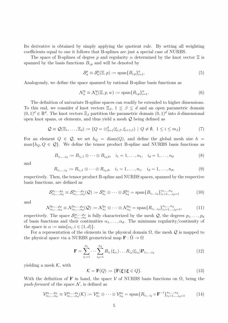
The space of B-splines of degree p and regularity α determined by the knot vector Ξ isspanned by the basis functions Bi,p and will be denoted by

Spα ≡ Spα(Ξ, p) := spanBi,pni=1. (5)

Analogously, we define the space spanned by rational B-spline basis functions as

N pα ≡ N p

α(Ξ, p, w) := spanRi,pni=1. (6)

The definition of univariate B-spline spaces can readily be extended to higher dimensions.To this end, we consider d knot vectors Ξβ, 1 ≤ β ≤ d and an open parametric domain(0, 1)d ∈ Rd. The knot vectors Ξβ partition the parametric domain (0, 1)d into d-dimensionalopen knot spans, or elements, and thus yield a mesh Q being defined as

Q ≡ Q(Ξ1, . . . ,Ξd) := Q = ⊗dβ=1(ξi,β, ξi+1,β) | Q 6= ∅, 1 ≤ i ≤ mβ (7)

For an element Q ∈ Q, we set hQ = diam(Q), and define the global mesh size h =maxhQ, Q ∈ Q. We define the tensor product B-spline and NURBS basis functions as

Bi1,...,id := Bi1,1 ⊗ · · · ⊗Bid,d, i1 = 1, . . . , n1, id = 1, . . . , nd (8)

andRi1,...,id := Ri1,1 ⊗ · · · ⊗Rid,d, i1 = 1, . . . , n1, id = 1, . . . , nd, (9)

respectively. Then, the tensor product B-spline and NURBS spaces, spanned by the respectivebasis functions, are defined as

Sp1,...,pdα1,...,αd

≡ Sp1,...,pdα1,...,αd

(Q) := Sp1α1⊗ · · · ⊗ Spdαd

= spanBi1...idn1,...,ndi1=1,...,id=1 (10)

andN p1,...,pdα1,...,αd

≡ N p1,...,pdα1,...,αd

(Q) := N p1α1⊗ · · · ⊗ N pd

αd= spanRi1...idn1,...,nd

i1=1,...,id=1, (11)

respectively. The space Sp1,...,pdα1,...,αd

is fully characterized by the mesh Q, the degrees p1, . . . , pdof basis functions and their continuities α1, . . . , αd. The minimum regularity/continuity ofthe space is α := minαi, i ∈ (1, d).

For a representation of the elements in the physical domain Ω, the mesh Q is mapped tothe physical space via a NURBS geometrical map F : Ω→ Ω

F =

n1∑i1=1

· · ·nd∑id=1

Ri1(ξi1) . . . Rid(ξid)Pi1,...,id (12)

yielding a mesh K, withK = F(Q) := F(ξ)|ξ ∈ Q. (13)

With the definition of F in hand, the space V of NURBS basis functions on Ω, being thepush-forward of the space N , is defined as

Vp1,...,pdα1,...,αd

≡ Vp1,...,pdα1,...,αd

(K) := Vp1α1⊗ · · · ⊗ Vpdαd

= spanRi1...id F−1n1,...,ndi1=1,...,id=1 (14)

5

In equation (12), P, denotes a homogeneous NURBS control point uniquely addressed in theNURBS tensor product mesh by its indices.

We assume that the parameterization F is invertible, with smooth inverse, on each elementQ ∈ Q. A mesh stack Qhh≤h0 , with affiliated spaces, can be constructed via knot insertionas described, e.g., in [7] from an initial coarse mesh Q0, with the global mesh size h pointingto a refinement level index.

3. Discrete approximation spaces

For an Isogeometric Analysis-based approximation of the unknowns of the PDEs consid-ered in this article (see Section 4), suitable B-spline or NURBS spaces, as defined in Section2, need to be specified. For the approximation of the velocity and pressure functions, weuse LBB-stable Taylor–Hood-like B-spline space pairs VTH

h /QTHh [6], being defined in the

parametric domain Ω as

VTHh ≡ VTH

h (p,α) = Sp1+1,p2+1α1,α2

= Sp1+1,p2+1α1,α2

× Sp1+1,p2+1α1,α2

,

QTHh ≡ QTH

h (p,α) = Sp1,p2α1,α2

.(15)

With the definition of finite dimensional spaces VTHh and QTH

h in hand, we proceed to con-struct the corresponding spaces VTH

h and QTHh in the physical domain Ω. Taylor–Hood spaces

VTHh /QTH

h can be mapped to the physical domain via a component-wise mapping [6] usingthe parameterization F : Ω→ Ω, i.e.

VTHh = v : v F ∈ VTH

h , QTHh = q : q F ∈ QTH

h . (16)

Note that these spaces may be alternatively set up to use NURBS instead of B-spline basisfunctions.Throughout this article, whenever a specific discrete B-spline or NURBS approximation spaceis addressed, we introduce – for the sake of brevity – the convention to refer to its presentationw.r.t. the parametric domain Ω, as shown in (15).

4. Governing equations

For stationary flow scenarios considered in this article, the governing equations to besolved are the steady-state incompressible Navier–Stokes equations represented in strongform as

−ν∇2v + (v · ∇)v +∇p = b in Ω, (17a)

∇ · v = 0 in Ω, (17b)

v = vD on ΓD, (17c)

−pn+ ν(n · ∇)v = t on ΓN , (17d)

where Ω ⊂ R2 is a bounded domain, ρ is the density, µ represents the dynamic viscosity,ν = µ/ρ is the kinematic viscosity, p = P/ρ denotes the normalized pressure, b is the bodyforce term, vD is the value of the velocity Dirichlet boundary conditions on the Dirichletboundary ΓD, t is the prescribed traction force on the Neumann boundary ΓN , and n is the

6

outward unit normal vector on the boundary. The kinematic viscosity and the density of thefluid are assumed to be constant. The first and second equations in (17) are the momentumand continuity equations, respectively.

Their continuous mixed variational formulation reads: Find v ∈ H1ΓD

(Ω) and p ∈L2(Ω)/R such that for all (w, q) ∈H1

0(Ω)× L2(Ω)/R it holdsa(w,v) + c(v;w,v) + b(w, p) = (w, b) + (w, t)ΓN

b(v, q) = 0,(18)

where L2 and H1 are Sobolev spaces as defined in [1].Replacement of the linear-, bilinear- and trilinear forms with their respective definitions

and application of integration by parts to (18) yields

ν

∫Ω

∇w : ∇v dΩ︸ ︷︷ ︸a(w,v)

+

∫Ω

w · v · ∇v dΩ︸ ︷︷ ︸c(v;w,v)

−∫

Ω

∇ ·wp dΩ︸ ︷︷ ︸b(w,p)

−∫

Ω

q∇ · v dΩ︸ ︷︷ ︸b(v,q)

=

∫Ω

w · b dΩ︸ ︷︷ ︸(w,b)

+

∫ΓN

νw · (∇v · n) dΓN −∫

ΓN

pw · n dΓN︸ ︷︷ ︸(w,t)ΓN

(19)

A downcast of the variational formulation (18) to the discrete level gives rise to the problemstatement

Find vh ∈H1ΓD

(Ω) ∩VTHh and ph ∈ L2(Ω)/R ∩QTH

h , such that

∀(wh, qh) ∈H10(Ω) ∩VTH

h × L2(Ω)/R ∩QTHh

a(wh,vh) + c(vh;wh,vh) + b(wh, ph) = (wh, bh) + (wh, th)ΓN

b(vh, qh) = 0,

(20)

with superscript h dubbing the mesh family index.In addition to the stationary flow around a circular obstacle model problem, we also

consider its unsteady counterpart (see Section 5.4). In the latter case, the unsteady incom-pressible Navier–Stokes equations, defined as

∂v

∂t− ν∇2v + (v · ∇)v +∇p = b in Ω×]0, T [, (21a)

∇ · v = 0 in Ω×]0, T [, (21b)

v = vD on ΓD×]0, T [, (21c)

−pn+ ν(n · ∇)v = t on ΓN×]0, T [, (21d)

v(x, 0) = v0(x) in Ω, (21e)

are solved in time, whereby the initial condition is required to satisfy ∇ · v0 = 0. The corre-sponding variational problem reads: Find v(x, t) ∈H1

ΓD(Ω)×]0, T [ and p(x, t) ∈ L2(Ω)×]0, T [,

such that for all (w, q) ∈H1Γ0

(Ω)× L2(Ω)/R it holds(w,vt) + a(w,v) + c(v;w,v) + b(w, p) = (w, b) + (w, t)ΓN

b(v, q) = 0(22)

7

Analogously, the semi-discretized counterpart of the variational formulation (22) reads:Find vh ∈H1

ΓD(Ω) ∩VTH

h ×]0, T [ and ph ∈ L2(Ω)/R ∩QTHh ×]0, T [, such that

∀(wh, qh) ∈H10(Ω) ∩VTH

h × L2(Ω)/R ∩QTHh

(wh,vht ) + a(wh,vh) + c(vh;wh,vh) + b(wh, ph) = (wh, bh) + (wh, th)ΓN

b(vh, qh) = 0

(23)

Since the nonlinear nature of the Navier–Stokes equations involves a great deal of complexity,we deliver in Section 4.1 an insight into the handling of the nonlinearity aspect.

4.1. Treatment of nonlinearity

The treatment of nonlinearity is showcased for the steady Navier–Stokes system as pre-sented in equation (17). This choice is motivated by the desire to keep this section as briefas possible. Note that the same principles for the treatment of nonlinearity apply to theunsteady Navier–Stokes system as well.

Let the nonlinear system (17) be presented in operator form as

L(u) = b with u = (v, p), (24)

and let it be disassembled as L = LA ⊕ LV ⊕ LG ⊕ LD, with operators LA = v · ∇v,LV = −ν∇2v, LG = ∇p and LD = ∇ · v.

In order to solve equation (24), an iterative procedure is required which, starting from aninitial guess for the unknowns, linearizes in every relaxation step the nonlinear system basedon the current solution un, and eventually solves the resulting system of linear equations.The iteration is advanced until a stopping criteria such as convergence is achieved.

Since the only nonlinear term in equation (24) is given by the advection operator LA, welinearize the latter via a generalized Taylor expansion of LA about the current iterate of thevelocity function vn and ignore higher order terms O(|δv|2). A Newton linearization of LAis derived as:

LA(v) = LA(vn) +dLA(vn + εδv)

dε

∣∣∣∣ε=0

+O(|δv|2)

≈ vn · ∇vn +d[(vn + εδv) · ∇(vn + εδv)]

dε

∣∣∣∣ε=0

= vn · ∇vn +d[vn · ∇(vn + εδv) + εδv · ∇(vn + εδv)]

dε

∣∣∣∣ε=0

= vn · ∇vn +d[vn · ∇vn + vn · ∇εδv + εδv · ∇vn + ε2δv · ∇δv]

dε

∣∣∣∣ε=0

= vn · ∇vn + vn · ∇δv + δv · ∇vn = vn · ∇vn + vn · ∇(v − vn) + (v − vn) · ∇vn= vn · ∇vn + vn · ∇v − vn · ∇vn + v · ∇vn − vn · ∇vn= vn · ∇v + v · ∇vn − vn · ∇vn

(25)Note that alternative linearizations are considered in different Picard iteration variants whereLA is taken either as LA ≈ vn · ∇v, LA ≈ v · ∇vn or LA ≈ vn · ∇vn.

8

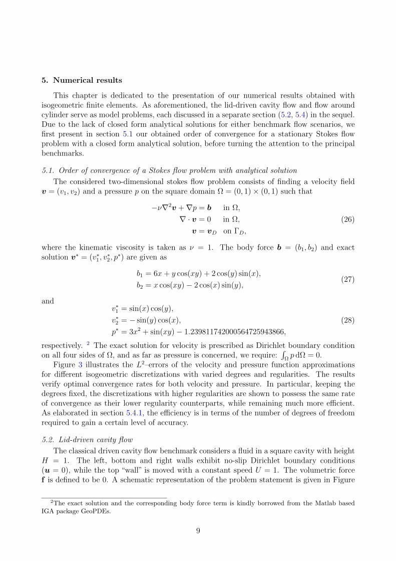
5. Numerical results

This chapter is dedicated to the presentation of our numerical results obtained withisogeometric finite elements. As aforementioned, the lid-driven cavity flow and flow aroundcylinder serve as model problems, each discussed in a separate section (5.2, 5.4) in the sequel.Due to the lack of closed form analytical solutions for either benchmark flow scenarios, wefirst present in section 5.1 our obtained order of convergence for a stationary Stokes flowproblem with a closed form analytical solution, before turning the attention to the principalbenchmarks.

5.1. Order of convergence of a Stokes flow problem with analytical solution

The considered two-dimensional stokes flow problem consists of finding a velocity fieldv = (v1, v2) and a pressure p on the square domain Ω = (0, 1)× (0, 1) such that

−ν∇2v +∇p = b in Ω,

∇ · v = 0 in Ω,

v = vD on ΓD,

(26)

where the kinematic viscosity is taken as ν = 1. The body force b = (b1, b2) and exactsolution v∗ = (v∗1, v

∗2, p∗) are given as

b1 = 6x+ y cos(xy) + 2 cos(y) sin(x),

b2 = x cos(xy)− 2 cos(x) sin(y),(27)

andv∗1 = sin(x) cos(y),

v∗2 = − sin(y) cos(x),

p∗ = 3x2 + sin(xy)− 1.239811742000564725943866,

(28)

respectively. 2 The exact solution for velocity is prescribed as Dirichlet boundary conditionon all four sides of Ω, and as far as pressure is concerned, we require:

∫Ωp dΩ = 0.

Figure 3 illustrates the L2–errors of the velocity and pressure function approximationsfor different isogeometric discretizations with varied degrees and regularities. The resultsverify optimal convergence rates for both velocity and pressure. In particular, keeping thedegrees fixed, the discretizations with higher regularities are shown to possess the same rateof convergence as their lower regularity counterparts, while remaining much more efficient.As elaborated in section 5.4.1, the efficiency is in terms of the number of degrees of freedomrequired to gain a certain level of accuracy.

5.2. Lid-driven cavity flow

The classical driven cavity flow benchmark considers a fluid in a square cavity with heightH = 1. The left, bottom and right walls exhibit no-slip Dirichlet boundary conditions(u = 0), while the top “wall” is moved with a constant speed U = 1. The volumetric forcef is defined to be 0. A schematic representation of the problem statement is given in Figure

2The exact solution and the corresponding body force term is kindly borrowed from the Matlab basedIGA package GeoPDEs.

9

1e-014

1e-012

1e-010

1e-008

1e-006

0.0001

0.01 0.1

∥ ∥ v−vh∥ ∥ L2

h

Ch3

Ch4

Ch5

S2,20,0

S3,30,0

S3,31,1

S4,40,0

S4,41,1

S4,42,2

1e-014

1e-012

1e-010

1e-008

1e-006

0.0001

0.01

0.01 0.1

∥ ∥ p−ph∥ ∥ L2

h

Ch2

Ch3

Ch4

S1,10,0

S2,20,0

S2,21,1

S3,30,0

S3,31,1

S3,32,2

Figure 3: Stokes flow: L2−errors of the velocity and pressure approximations obtained with isogeometricdiscretizations of various degrees and regularities.

Figure 4: Sketch of lid-driven cavity model.

4. At the upper left and right corners, there is a discontinuity in the velocity boundaryconditions producing a singularity in the pressure field at those corners. They can either beconsidered as part of the upper boundary or as part of the vertical walls. The former caseis referred to as the “leaky” cavity rendering the latter “non-leaky”. As Dirichlet boundaryconditions are imposed everywhere on the boundary (ΓN = ∅), pressure is in equation (17)only present by its gradient, and thus it is only determined up to an arbitrary constant. Fora unique definition of the discrete pressure field, it is usual to either impose its average (e.g.∫

Ωp dΩ = 0) or fix its value at one point. We follow the latter approach and fix the value of

the discrete pressure field with the value 0 at the lower left corner of the cavity.Our results, obtained with various B-spline space-based discretizations for three consec-

utive mesh refinement levels h ∈ [1/32, 1/64, 1/128] of unstretched meshes, are comparedto classical reference results from the literature such as those of Ghia [12] using a second-order upwind finite difference method on a stretched mesh with 1922 grid points. Moreover,additional comparisons are done with highly accurate, spectral method-based (ChebyshevCollocation) solutions of Botella [4] that show convergence up to seven digits. Furthermore,whenever comparable data is provided, results of two recently published articles [9, 21], bothapplying IGA to the cavity flow problem, are addressed. All our computations for cavity floware performed without taking any stabilization measures for the advection term. As for theNewton iteration, the stopping criterion is considered fulfilled when the euclidean norm of

10

the residual of equation (17) drops below the bound 10−10.Using the B-spline space pair S2,2

0,0×S1,10,0 for the approximation of the velocity and pressure

functions, we present in Figure 5 stream function (ψ) and vorticity (ω) profiles computed forReynolds (Re) numbers 100, 400 and 1000. Given the circumstance that profiles for ψ and ω

Figure 5: Stream function (top) and vorticity (bottom) profiles for Reynolds 100, 400 and 1000 from left toright. Respective contour ranges for stream function and vorticity: ψiso ∈ [−10−10, 3× 10−3], ωiso ∈ [−5, 3].Discretization: S2,2

0,0 × S1,10,0 . h = 1/64 (Refinement level: 6). Number of degrees of freedom: 37507.

are provided by all mentioned references in graphical form only, we conclude the discussionon stream function and vorticity profiles with the note that visually both profiles match thecorresponding profiles in the literature very well.

Remark 1. The approach we follow for the computation of the stream function in 2D, isbased on solving a Poisson equation for ψ with the scalar 2D vorticity function on the righthand side:

−∇2ψ = ω

ω = ∇× v =∂v

∂x− ∂u

∂y

(29)

Equation (29) is easily solvable via FEM/IGA when formulated as a unique boundary valueproblem in the domain Ω enclosed by the boundary Γ. We set Dirichlet boundary conditionsof 0 on the entire boundary when solving for ψ.

11

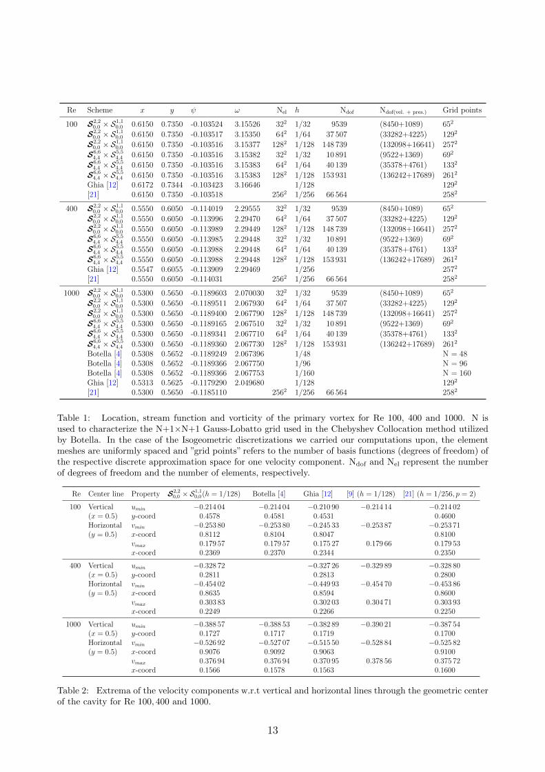
In Table 1, stream function and vorticity values at the center of the main vortex arepresented for Reynolds numbers 100, 400, and 1000 and compared to the reference values ofGhia, Botella, and the stream function-based Galerkin IGA scheme of [21]. For each Reynoldsnumber we present values for two different Isogeometric discretizations (S2,2

0,0×S1,10,0 and S6,6

4,4×S5,5

4,4 ), and additionally vary for the latter the mesh refinement among three consecutive stages.Note that in Botella’s case the flow is reversed, that is, the velocity at the upper boundary isu = (−1, 0). However, the flow attributes obtained are mirror-symmetric and comparable tothose of older references, such as Ghia’s. Botella’s results, based on a Chebyshev Collocationmethod with polynomial degrees as high as 160, are considered highly accurate and motivatedthe usage of a high degree B-splines space pair such as S6,6

4,4 × S5,54,4 . On a general note, for

all Reynolds numbers under consideration, our results are considered converged and in goodagreement with the references. Without any exception, both Isogeometric discretizationsyield values for the position of the main vortex itself, and stream function and vorticity at themain vortex which are closer to Botella’s than Ghia’s results. A comparison with the streamfunction formulation based IGA results of [21] reveals matching positions of the main vortexup to four decimal digits for all Reynolds numbers, discretizations, and mesh refinementlevels. Our stream function values match [21] very well, but are shown for Re 1000 to beminimally closer to Botella’s results for both discretizations and all mesh refinement levels.Coming up next, we depict our approximations of the u- and v-velocity components alongvertical and horizontal lines through the geometric center of the cavity, respectively. Thecorresponding profiles obtained with a S2,2

0,0 × S1,10,0 discretization for h ∈ [1/32, 1/64, 1/128]

are presented graphically alongside those of Ghia in Figure 6. Except for one irregularitywith respect to the v-velocity component (see Fig. 6) computations in the Re 400 case, theconverged profiles follow the reference data of Ghia and reflect the profiles presented in theisogeometric references [9, 21].

The extrema of the velocity components along horizontal and vertical lines through thegeometric center of the cavity are listed in Table 2 and compared to both isogeometric and theclassical references. As can be seen from the tabulated data, the results of the isogeometricTaylor–Hood discretization are closest to those of Botella obtained with a spectral method.

In addition to the presented results regarding the S2,20,0 × S1,1

0,0 discretization, we deliver

additional ones associated to both an approximation space pair with higher regularity S6,64,4 ×

S5,54,4 (C4) and a reversed flow direction (u = (−1, 0)), such as the setup used by Botella. A

graphical representation of converged velocity component and vorticity data approximatedin the above described C4 space pair, exhibiting excellent agreement with the ones stemmingfrom Botella’s spectral method, is illustrated in Figure 7.

5.3. Regularized driven cavity flowIn the regularized lid-driven cavity flow scenario as described in [5], the flow domain

is a unit square exhibiting no-slip Dirichlet boundary conditions at the vertical and lowerhorizontal boundaries. In order to avoid the pressure singularities in the upper left andright domain corners involved with the regular lid-driven cavity flow scenario, the regularizedlid-driven cavity flow problem defines the following velocity profile on the top boundary

ulid = [−16x2(1− x)2, 0]. (30)

In addition to the study of local quantities, it is reasonable to extend the analysis to globalquantities. Towards this end, we fix the value of the discrete pressure field at the lower

12

Re Scheme x y ψ ω Nel h Ndof Ndof(vel. + pres.) Grid points

100 S2,20,0 × S1,1

0,0 0.6150 0.7350 -0.103524 3.15526 322 1/32 9539 (8450+1089) 652

S2,20,0 × S1,1

0,0 0.6150 0.7350 -0.103517 3.15350 642 1/64 37 507 (33282+4225) 1292

S2,20,0 × S1,1

0,0 0.6150 0.7350 -0.103516 3.15377 1282 1/128 148 739 (132098+16641) 2572

S6,64,4 × S5,5

4,4 0.6150 0.7350 -0.103516 3.15382 322 1/32 10 891 (9522+1369) 692

S6,64,4 × S5,5

4,4 0.6150 0.7350 -0.103516 3.15383 642 1/64 40 139 (35378+4761) 1332

S6,64,4 × S5,5

4,4 0.6150 0.7350 -0.103516 3.15383 1282 1/128 153 931 (136242+17689) 2612

Ghia [12] 0.6172 0.7344 -0.103423 3.16646 1/128 1292

[21] 0.6150 0.7350 -0.103518 2562 1/256 66 564 2582

400 S2,20,0 × S1,1

0,0 0.5550 0.6050 -0.114019 2.29555 322 1/32 9539 (8450+1089) 652

S2,20,0 × S1,1

0,0 0.5550 0.6050 -0.113996 2.29470 642 1/64 37 507 (33282+4225) 1292

S2,20,0 × S1,1

0,0 0.5550 0.6050 -0.113989 2.29449 1282 1/128 148 739 (132098+16641) 2572

S6,64,4 × S5,5

4,4 0.5550 0.6050 -0.113985 2.29448 322 1/32 10 891 (9522+1369) 692

S6,64,4 × S5,5

4,4 0.5550 0.6050 -0.113988 2.29448 642 1/64 40 139 (35378+4761) 1332

S6,64,4 × S5,5

4,4 0.5550 0.6050 -0.113988 2.29448 1282 1/128 153 931 (136242+17689) 2612

Ghia [12] 0.5547 0.6055 -0.113909 2.29469 1/256 2572

[21] 0.5550 0.6050 -0.114031 2562 1/256 66 564 2582

1000 S2,20,0 × S1,1

0,0 0.5300 0.5650 -0.1189603 2.070030 322 1/32 9539 (8450+1089) 652

S2,20,0 × S1,1

0,0 0.5300 0.5650 -0.1189511 2.067930 642 1/64 37 507 (33282+4225) 1292

S2,20,0 × S1,1

0,0 0.5300 0.5650 -0.1189400 2.067790 1282 1/128 148 739 (132098+16641) 2572

S6,64,4 × S5,5

4,4 0.5300 0.5650 -0.1189165 2.067510 322 1/32 10 891 (9522+1369) 692

S6,64,4 × S5,5

4,4 0.5300 0.5650 -0.1189341 2.067710 642 1/64 40 139 (35378+4761) 1332

S6,64,4 × S5,5

4,4 0.5300 0.5650 -0.1189360 2.067730 1282 1/128 153 931 (136242+17689) 2612

Botella [4] 0.5308 0.5652 -0.1189249 2.067396 1/48 N = 48Botella [4] 0.5308 0.5652 -0.1189366 2.067750 1/96 N = 96Botella [4] 0.5308 0.5652 -0.1189366 2.067753 1/160 N = 160Ghia [12] 0.5313 0.5625 -0.1179290 2.049680 1/128 1292

[21] 0.5300 0.5650 -0.1185110 2562 1/256 66 564 2582

Table 1: Location, stream function and vorticity of the primary vortex for Re 100, 400 and 1000. N isused to characterize the N+1×N+1 Gauss-Lobatto grid used in the Chebyshev Collocation method utilizedby Botella. In the case of the Isogeometric discretizations we carried our computations upon, the elementmeshes are uniformly spaced and ”grid points” refers to the number of basis functions (degrees of freedom) ofthe respective discrete approximation space for one velocity component. Ndof and Nel represent the numberof degrees of freedom and the number of elements, respectively.

Re Center line Property S2,20,0 × S1,1

0,0 (h = 1/128) Botella [4] Ghia [12] [9] (h = 1/128) [21] (h = 1/256, p = 2)

100 Vertical umin −0.214 04 −0.214 04 −0.210 90 −0.214 14 −0.214 02(x = 0.5) y-coord 0.4578 0.4581 0.4531 0.4600Horizontal vmin −0.253 80 −0.253 80 −0.245 33 −0.253 87 −0.253 71(y = 0.5) x-coord 0.8112 0.8104 0.8047 0.8100

vmax 0.179 57 0.179 57 0.175 27 0.179 66 0.179 53x-coord 0.2369 0.2370 0.2344 0.2350

400 Vertical umin −0.328 72 −0.327 26 −0.329 89 −0.328 80(x = 0.5) y-coord 0.2811 0.2813 0.2800Horizontal vmin −0.454 02 −0.449 93 −0.454 70 −0.453 86(y = 0.5) x-coord 0.8635 0.8594 0.8600

vmax 0.303 83 0.302 03 0.304 71 0.303 93x-coord 0.2249 0.2266 0.2250

1000 Vertical umin −0.388 57 −0.388 53 −0.382 89 −0.390 21 −0.387 54(x = 0.5) y-coord 0.1727 0.1717 0.1719 0.1700Horizontal vmin −0.526 92 −0.527 07 −0.515 50 −0.528 84 −0.525 82(y = 0.5) x-coord 0.9076 0.9092 0.9063 0.9100

vmax 0.376 94 0.376 94 0.370 95 0.378 56 0.375 72x-coord 0.1566 0.1578 0.1563 0.1600

Table 2: Extrema of the velocity components w.r.t vertical and horizontal lines through the geometric centerof the cavity for Re 100, 400 and 1000.

13

0.0 0.2 0.4 0.6 0.8 1.0x

−0.3

−0.2

−0.1

0.0

0.1

0.2

v

v-velocity over x (Re 100)ghiah = 1/32

h = 1/64

h = 1/128

0.83668 0.83672 0.83676

−0.24812

−0.24808

−0.24804

−0.4 −0.2 0.0 0.2 0.4 0.6 0.8 1.0 1.2u

0.0

0.2

0.4

0.6

0.8

1.0

y

u-velocity over y (Re 100)

ghiah = 1/32

h = 1/64

h = 1/128

−0.192970 −0.192955

0.35976

0.35978

0.0 0.2 0.4 0.6 0.8 1.0x

−0.5

−0.4

−0.3

−0.2

−0.1

0.0

0.1

0.2

0.3

0.4

v

v-velocity over x (Re 400)ghiah = 1/32

h = 1/64

h = 1/128

0.403980 0.403985

0.17222

0.17224

0.17226

−0.4 −0.2 0.0 0.2 0.4 0.6 0.8 1.0 1.2u

0.0

0.2

0.4

0.6

0.8

1.0y

u-velocity over y (Re 400)

ghiah = 1/32

h = 1/64

h = 1/128

0.21428 0.21430

0.77810

0.77815

0.0 0.2 0.4 0.6 0.8 1.0x

−0.6

−0.4

−0.2

0.0

0.2

0.4

v

v-velocity over x (Re 1000)ghiah = 1/32

h = 1/64

h = 1/128

0.39028 0.39032

0.14365

0.14380

0.14395

−0.4 −0.2 0.0 0.2 0.4 0.6 0.8 1.0 1.2u

0.0

0.2

0.4

0.6

0.8

1.0

y

u-velocity over y (Re 1000)

ghiah = 1/32

h = 1/64

h = 1/128

0.2296720.229678

0.767200

0.767225

Figure 6: Profiles of v- and u-velocity components over horizontal and vertical lines through geometric centerof the cavity for Re 100, 400 and 1000. Discretization: S2,2

0,0 × S1,10,0 ; See Table 1 for the number of degrees offreedom.

left domain node with p = 0, and compute the global quantities kinetic energy (E) andenstrophy (Z)

E =1

2

∫Ω

‖u‖2 dx, Z =1

2

∫Ω

ω2 dx, (31)

14

0.0 0.2 0.4 0.6 0.8 1.0x

−0.6

−0.4

−0.2

0.0

0.2

0.4

v

v-velocity over x (Re 1000)Botella N = 160

h = 1/32

h = 1/64

h = 1/128

0.499996 0.500000

0.025798

0.025804

0.025810

−1.0 −0.8 −0.6 −0.4 −0.2 0.0 0.2 0.4u

0.0

0.2

0.4

0.6

0.8

1.0

y

u-velocity over y (Re 1000)

Botella N = 160

h = 1/32

h = 1/64

h = 1/128

−0.188677 −0.188674

0.73440

0.73442

0.0 0.2 0.4 0.6 0.8 1.0ω

−10

−8

−6

−4

−2

0

2

4

x

Vorticity over x (Re 1000)

Botella N = 160

h = 1/32

h = 1/64

h = 1/1280.4999990 0.5000005 0.5000020

2.0670

2.0671

2.0672

−5 0 5 10 15 20y

0.0

0.2

0.4

0.6

0.8

1.0ω

Vorticity over y (Re 1000)

Botella N = 160

h = 1/32

h = 1/64

h = 1/128

2.09095 2.09110 2.09125

0.73440

0.73441

Figure 7: Profiles of v- and u-velocity components and vorticity over horizontal and vertical lines throughgeometric center of the cavity for Re 1000. Discretization: S6,6

4,4 ×S5,54,4 ; See Table 1 for the number of degreesof freedom.

where ω = ∂v∂x− ∂u

∂ydenotes the scalar vorticity in 2D. In Table 3 we compare our results

for Reynolds number 1000, computed on unstretched meshes, to the results of Bruneau [5]using finite differences and a 3Q2P1 finite element discretization, published in [17]. All threeisogeometric finite element pairs in charge produce very satisfying results for kinetic energyand enstrophy obviously well integrating with references. Selecting the isogeometric finiteelement pair with the lowest degree S2,2

0,0 × S1,10,0 , we compare in Table 4 the approximated

kinetic energy for three mesh refinement levels with data [17] obtained from three differentfinite element discretizations, namely4, Q1Q0, Q2P1, and5 W-LSFE Q2, all available in theFeatFlow6 package. As can be deduced from the tabulated data, our results are charac-terized by both a high accuracy and a satisfactory convergence for all considered Reynoldsnumbers.

3Velocity: Biquadratic, continuous; Pressure: Linear (value and two partial derivatives), discontinuous4Velocity: Bilinear, rotated; Pressure: Constant.5Biquadratic Least-Square finite elements.6www.featflow.de.

15

Scheme Kinetic Energy Enstrophy Nel h Ndof Ndof(vel. + pres.) Grid points

S2,20,0 × S1,1

0,0 0.022909 4.80747 322 1/32 9539 (8450+1089) 652

0.022778 4.82950 642 1/64 37507 (33282+4225) 1292

0.022767 4.83041 1282 1/128 148739 (132098+16641) 2572

0.022767 4.83043 2562 1/256 592387 (526338+66049) 5132

S3,30,0 × S2,2

0,0 0.022905 4.81717 162 1/16 5891 (4802+1089) 492

0.022773 4.83079 322 1/32 23043 (18818+4225) 972

0.022767 4.83047 642 1/64 91139 (74498+16641) 1932

0.022767 4.83042 1282 1/128 362499 (296450+66049) 3852

S3,31,1 × S2,2

1,1 0.022777 4.82954 322 1/32 9868 (8712+1156) 662

0.022767 4.83048 642 1/64 38156 (33800+4356) 1302

0.022767 4.83046 1282 1/128 150028 (133128+16900) 2582

Ref. [5] (Bruneau) 0.021564 4.6458 642

0.022315 4.7711 1282

0.022542 4.8123 2562

0.022607 4.8243 5122

Ref. [17] (Q2P1 FE) 0.022778 4.82954 642 1/640.022768 4.83040 1282 1/1280.022766 4.83050 2562 1/256

Table 3: Kinetic energy and enstrophy of the regularized cavity flow for Reynolds 1000. In the case ofIsogeometric discretizations, ”grid points” refers to the number of basis functions (degrees of freedom) of therespective discrete approximation space for one velocity component.

Re h S2,20,0 × S1,1

0,0 Q1Q0 FE Q2P1 FE W-LSFE Q2 [17]

1 1/64 1.862439E-02 1.860621E-02 1.862439E-02 1.862353E-021/128 1.862438E-02 1.861982E-02 1.862438E-02 1.862432E-021/256 1.862438E-02 1.862324E-02 1.862438E-02 1.862438E-02

400 1/64 2.131703E-02 2.148649E-02 2.131707E-02 2.133053E-021/128 2.131547E-02 2.136484E-02 2.131547E-02 2.131581E-021/256 2.131537E-02 2.132812E-02 2.131529E-02 2.131537E-02

1000 1/64 2.277788E-02 2.409799E-02 2.277778E-02 2.552796E-021/128 2.276761E-02 2.305179E-02 2.276761E-02 2.287704E-021/256 2.276692E-02 2.282649E-02 2.276582E-02 2.277389E-02

Table 4: Convergence of approximated kinetic energy for the regularized cavity flow problem.

16

5.4. Flow around cylinder

Flow around an obstacle in a channel is a prominent benchmark model for the assessmentof flow affiliated attributes, produced by a numerical technique in charge with the analysis.Following the lines of [10, 11, 16, 19], we choose as flow scenarios a steady Re 20 and atransient Re 100 2D channel flow the details of which are presented in sections 5.4.1 and5.4.2, respectively. The underlying geometry for both cases is depicted in Figure 8 and isdefined as a pipe where a circular cylinder of radius r = 0.05 has been cut out, that is,Ω = (0, 2.2)× (0, 0.41) \Br(0.2, 0.2)7. The cylinder is centered around (x, y) = (0.2, 0.2).

2.2

0.2

0.21

0.2

Figure 8: Computational domain for flow around cylinder.

5.4.1. DFG benchmark 2D-1

In DFG benchmark 2D-1 the fluid density and kinematic viscosity are taken as ρ = 1and ν = 0.001. We require no-slip boundary conditions for the lower and upper walls Γ1 =(0, 2.2) × 0 and Γ3 = (0, 2.2) × 0.41, as well as for the boundary S = ∂Br(0.2, 0.2):u|Γ1 = u|Γ3 = u|S = 0. On the left edge Γ4 = 0 × (0, 0.41), a parabolic inflow profile is

prescribed, u(0, y) =(

4Uy(0.41−y)0.412 , 0

), with a maximum velocity U = 0.3. On the right edge

Γ2 = 2.2 × (0, 0.41), “do-nothing” boundary conditions, −pn + ν(n · ∇)v = 0, define theoutflow, with n denoting the outer normal vector. For a maximum velocity of U = 0.3,the parabolic profile results in a mean velocity U = 2

3· 0.3 = 0.2. The flow configurations

characteristic length D = 2 · 0.05 = 0.1 is the diameter of the object perpendicular to theflow direction. This particular problem configuration yields Reynolds number Re = UD

ν=

0.2·0.10.001

= 20 for which the flow is considered stationary.Following the above setup for Re = 20, we present the results of the application of

Isogeometric Analysis, with particular emphasis on the approximated drag and lift valuesrelated to the entire obstacle boundary.

With S dubbing the surface of the obstacle, nS its inward pointing unit normal vectorw.r.t. the computational domain Ω, tangent vector τ := (ny,−nx)T and uτ := u · τ , thedrag and lift forces are given by

FD =

∫S

(ρν∂uτ∂nS

ny − pnx)ds, FL = −

∫S

(ρν∂uτ∂nS

nx + pny

)ds

CD =2

ρU2DFD, CL =

2

ρU2DFL,

(32)

where CD and CL are the drag and lift coefficients, and u and p represent velocity andpressure, respectively [15, 19]. We follow, however, the alternative approach of [15, 23] and

7The presented measures for the domain definition are in meters.

17

evaluate a volume integral for the approximations of the drag and lift coefficients. Givenfilter functions

vd|S = (1, 0)T ,vd|Ω−S = 0 vl|S = (0, 1)T ,vl|Ω−S = 0, (33)

the corresponding volume integral expressions read

CD = − 2

ρU2D[(ν∇u,∇vd)− (p,∇ · vd)]

CL = − 2

ρU2D[(ν∇u,∇vl)− (p,∇ · vl)] ,

(34)

with (·, ·) denoting the L2(Ω) inner product. Note that in the discrete setting, we use therespective interpolants of the discontinuous filter functions vd and vl.

We model the computational domain as a multi-patch NURBS mesh (see Fig. 9), due tothe fact that the parametric space of a multi-variate NURBS patch exhibits a tensor productstructure, and thus is not mappable to any other topology than a cube in the respectiveN -dimensional space. However, the multi-patch setup yields a perfect mathematical repre-sentation of the circular boundary and in particular avoids its approximation with straightline segments. Note that each quarter of the “obstacle circle” can be modeled exactly witha NURBS curve of degree 2 and just 3 control points. Since the ability to exactly representconical sections is restricted to rational B-splines only, a NURBS mesh comes in handy forthe modeling of the computational domain. In order to impose the parabolic inflow condition,

Figure 9: Multi-patch NURBS mesh for flow around cylinder at refinement level 3. Each uniquely coloredinitial 1×1 element patch has been refined three times, giving rise to 8×8 elements in each patch, eventually.

we perform a finite element L2–projection∫Γ4

(f − Phf) w dΓ4 = 0, ∀w ∈ Wh (35)

of the inflow profile f on the control points associated with the left boundary (Γ4) in Fig. 9,whereby Wh denotes a suitable discrete space of weighting/test functions.

For the approximation of drag, lift, and pressure drop we use two different isogeometricdiscretizations, namely, S3,3

0,0 × S2,20,0 and S3,3

1,1 × S2,21,1 , and compare their results for different

mesh refinement levels with a reference solution computed with high order spectral methods[16]. The choice of these two isogeometric discretizations is explained by the fact that werequire the discrete pressure approximation space to have the same degrees and regularitiesas the geometry. Since modeling one quarter of the obstacle circle requires a NURBS curve of

18

at least degree 2, the degrees of the discrete pressure approximation space reflect this setting.The degrees and regularities of the discrete velocity approximation space eventually followfrom the constraints defined by Taylor–Hood elements (see e.g. [6]). In fact, given an initialdiscrete pressure space, we use k-refinement [7] followed by knot insertion to setup a desiredTaylor–Hood space of higher degree and possibly lower regularity.

We refer to table 5 for a compilation of the approximated forces for different mesh refine-ment levels. Our results exhibit high accuracy on the highest mesh refinement level (L8),since a comparison with the reference data reveals 4, 6, and 7 matching decimal digits fordrag, lift, and pressure drop, respectively. Moreover, starting with mesh refinement level 6,

Scheme CD CL ∆p Ndof Nel Level

S3,30,0 × S2,2

0,0 5.645768 0.0067650 0.11675114 8832 384 L3

S3,30,0 × S2,2

0,0 5.594618 0.0095045 0.11733243 34560 1536 L4

S3,30,0 × S2,2

0,0 5.582119 0.0104074 0.11749107 136704 6144 L5

S3,30,0 × S2,2

0,0 5.579918 0.0105860 0.11751658 543744 24576 L6

S3,30,0 × S2,2

0,0 5.579588 0.0106143 0.11751977 2168832 98304 L7

S3,30,0 × S2,2

0,0 5.579543 0.0106183 0.11752012 8663040 393216 L8

S3,31,1 × S2,2

1,1 5.647333 0.0066836 0.11633509 4212 384 L3

S3,31,1 × S2,2

1,1 5.594742 0.0095065 0.11723232 15300 1536 L4

S3,31,1 × S2,2

1,1 5.582148 0.0104082 0.11749043 58212 6144 L5

S3,31,1 × S2,2

1,1 5.579918 0.0105861 0.11751770 226980 24576 L6

S3,31,1 × S2,2

1,1 5.579588 0.0106143 0.11751993 896292 98304 L7

S3,31,1 × S2,2

1,1 5.579543 0.0106183 0.11752014 3562020 393216 L8

Ref. [11, 16] 5.57953523384 0.010618948146 0.11752016697

Table 5: Approximation results for drag, lift and pressure drop (∆p).

the approximated drag and lift coefficients of both isogeometric discretizations are, except forone irregularity, identical with respect to the displayed number of decimal digits. This resultis remarkable and advocates the usage of the discretization with higher continuity, since thenumber of degrees of freedoms it requires to reach the same accuracy on refinement level 7is approximately 42% of its C0 counterpart. The development of this “gain” is illustrated inFigure 10 for mesh refinement levels one to eight. Comparing the presented C0– and C1–based

1 2 3 4 5 6 7 8L

40

45

50

55

60

65

70

%

Figure 10: Percentage ratio (DOFs(S3,31,1 × S2,21,1 , L)/DOFs(S3,3

0,0 × S2,20,0 , L)× 100) of the number of degrees of

freedom of the C1 discretization and the C0 discretization for each mesh refinement level L of the flow aroundcylinder mesh. Table 5 lists the number of degrees of freedom for each L.

isogeometric discretizations, one observes in the former case an increased amount of degrees of

19

freedom on the same number of elements. This is due to the fact that the discretization withthe lower continuity exhibits an increased internal knot multiplicity which in turn implies alarger number of basis functions. This leads on mesh refinement levels ≥ 1 to numbers ofdegrees of freedom which are not well comparable between the two IGA-based discretizations.However, a linear interpolation of the the drag and lift percent errors, as depicted in Figure11, bears testimony to the accuracy-wise superiority of the high continuity C1 approach. The

0.0001

0.001

0.01

0.1

1

10

1000 10000 100000 1e+06 1e+07

CD

%-e

rror

Degrees of freedom

S3,30,0 × S2,2

0,0

S3,31,1 × S2,2

1,1

0.001

0.01

0.1

1

10

100

1000 10000 100000 1e+06 1e+07

CL%

-err

or

Degrees of freedom

S3,30,0 × S2,2

0,0

S3,31,1 × S2,2

1,1

Figure 11: Sectional view of drag and lift percent errors. Discretizations: S3,30,0 × S2,20,0 ; S3,3

1,1 × S2,21,1 .

semantics of superiority is in terms of gained accuracy with respect to the number of degreesof freedom invested.

Remark 2. We point out that, regardless of the regularity, the support of univariate B-splineand NURBS basis functions of degree p is always p + 1 knot spans. In 1D, the number offunctions that any given function shares support with (including itself) is 2p + 1, and themaximum bandwidth of a stiffness matrix produced with IGA in a Galerkin framework, isalways 2p+ 1 regardless of the smoothness of the basis functions (C0 or Cp−1 continuous).

Generally, it should be noted that the solutions we obtained with the C>0 approaches stillreduce to C0 at patch boundaries. There exist means to overcome this deficiency [7], none ofwhich have been considered in this study, though. Besides, for all simulations performed, weutilized standard quadrature rules (#cub.pts = p + 1), certainly not the most efficient rulesat Isogeometric Analysis’ disposal. Finally, for the nonlinear iteration the same stoppingcriterion as in the lid-driven cavity case is used, that is, it is halted as soon as the euclideannorm of the residual of equation (17) is below 10−10.

5.4.2. DFG benchmark 2D-2

In the following we turn our attention to the DFG benchmark 2D-2 [10, 19] definingan unsteady configuration for the flow around cylinder scenario on the same computationaldomain as in the DFG benchmark 2D-1 case. The setup aims to simulate the time-periodic behavior of a fluid in a 2D pipe with a circular obstacle. The attention is turned inparticular to the resulting drag, lift, and pressure drop profiles which are shown to have anoscillating and periodic structure. These profiles are analyzed with respect to their frequency,amplitude, minimum, maximum, and mean values.

20

In this benchmark, the maximum velocity of the parabolic inflow profile amounts to

U = 1.5, yielding Re = UDν

=23· 32·0.1

0.001= 100. In order to obtain a time profile for the drag, lift,

and pressure drop coefficients, we use again the NURBS mesh shown in Figure 9 and applyIsogeometric Analysis to the unsteady incompressible Navier–Stokes equations (21), usingthe Taylor–Hood B-spline spaces QTH

h = S2,20,0 and VTH

h = S3,30,0 for pressure and velocity,

respectively. Treating Eq. (21) as is, i.e. without the application of any operator splittingtechniques, corresponds to solving in a fully coupled manner since we solve for all unknownfunctions simultaneously.

For the time discretization, the single step θ-scheme with θ = 0.5 is used, leading to the2nd order accurate implicit Crank–Nicolson scheme [22]. Together with the space discretiza-tion, the following nonlinear block system has to be solved in every time step(

1∆tM + θ(D + C(vn+1)) G

GT 0

)(vn+1

pn+1

)=

(1

∆tM− (1− θ)(D + C(vn)) 0

0 0

)(vn

pn

)+ θfn+1 + (1− θ)fn.

(36)In the above system, M,D,C,G, and GT denote the mass, diffusion, advection, gradient,and divergence matrices, respectively. The body forces are discretized into f . As far as thetreatment of nonlinearity is concerned, for every time step, the nonlinear iteration is advanceduntil the nonlinear residual of equation (36) is reduced to 10−3 of its initial value.

For all mesh levels we performed an intermediate computation with a very coarse timestep (∆t = 1/10) for a total time of 35 simulation seconds. This yielded a profile which wetook as an initial solution for the final computation with a finer time step, scheduled for 30simulation seconds.

Exemplary sectional views of the approximated drag, lift and pressure drop time profilesfor three consecutive mesh refinement levels and a time step size of ∆t = 1/400 are presentedin Figure 12. Note that the depicted time interval is chosen arbitrarily after the drag and liftprofiles were considered fully developed. In addition, the curves have been shifted in time inorder to facilitate comparison.

Tables 6 and 7 supply minimum, maximum, mean, and amplitude values for the approx-imated drag and lift coefficients of different mesh refinement levels.

Level ∆t min-CD(Abs-Err,%-Err) max-CD(Abs-Err,%-Err) mean-CD(Abs-Err,%-Err) amp-CD(Abs-Err,%-Err)

L4 1/400 3.2216 (0.0573, 1.81) 3.2857 (0.0583, 1.81) 3.2536 (0.0578, 1.81) 0.0642 (0.0011, 1.62)L5 1/400 3.1755 (0.0112, 0.35) 3.2392 (0.0118, 0.37) 3.2074 (0.0116, 0.36) 0.0637 (0.0006, 0.94)L6 1/400 3.1665 (0.0022, 0.07) 3.2300 (0.0026, 0.08) 3.1983 (0.0025, 0.08) 0.0635 (0.0004, 0.58)

Ref. [10] 3.1643 3.2274 3.1958 0.0631

Table 6: min, max, mean, and amplitude of the drag coefficient values (including their absolute and percenterrors) for different mesh levels.

Our results are shown to converge to the most accurate available results of an alternativenumerical simulation [10] using Q2P1 finite elements (without stabilization) for space dis-cretization and Crank–Nicolson scheme for time discretization. Note that the absolute errorof the lift coefficient is at level L4 already one order of magnitude smaller than that of thedrag coefficient. However, the min/max values of the drag coefficient exhibit a significantlyfaster convergence than those of the lift coefficient.

21

3.16

3.18

3.2

3.22

3.24

3.26

3.28

3.5 3.55 3.6 3.65 3.7 3.75 3.8 3.85

dra

g

t(sec)

time profile of drag

L4,∆t = 1/400L5,∆t = 1/400L6,∆t = 1/400

Ref.

3.21

3.22

3.23

3.24

3.25

3.26

3.27

3.28

3.29

3.6 3.62 3.64 3.66 3.68 3.7 3.72 3.74dra

g

t(sec)

time profile of drag

L4,∆t = 1/400L5,∆t = 1/400L6,∆t = 1/400

Ref.

-1

-0.5

0

0.5

1

3.6 3.65 3.7 3.75 3.8 3.85 3.9

lift

t(sec)

time profile of lift

L4,∆t = 1/400L5,∆t = 1/400L6,∆t = 1/400

Ref.

0.96

0.965

0.97

0.975

0.98

0.985

0.99

0.995

3.735 3.74 3.745 3.75 3.755 3.76 3.765 3.77

lift

t(sec)

time profile of lift

L4,∆t = 1/400L5,∆t = 1/400L6,∆t = 1/400

Ref.

2.42

2.43

2.44

2.45

2.46

2.47

2.48

2.49

2.5

2.51

3.1 3.15 3.2 3.25 3.3 3.35 3.4

pre

ssure

dro

p

t(sec)

time profile of pressure drop

L4,∆t = 1/400L5,∆t = 1/400L6,∆t = 1/400

Ref.

2.496

2.498

2.5

2.502

2.504

2.506

2.508

2.51

3.225 3.23 3.235 3.24 3.245 3.25 3.255 3.26 3.265 3.27 3.275

pre

ssure

dro

p

t(sec)

time profile of pressure drop

L4,∆t = 1/400L5,∆t = 1/400L6,∆t = 1/400

Ref.

Figure 12: Sectional views of drag, lift, and pressure drop coefficient time profiles for Re 100 computed witha S3,3

0,0 ×S2,20,0 discretization and a time step of ∆t = 1/400. These profiles are shown to converge to Q2P1 FEbased reference [10] results. The numbers of degrees of freedom are given in Table 5.

22

Level ∆t min-CL(Abs-Err,%-Err) max-CL(Abs-Err,%-Err) mean-CL(Abs-Err,%-Err) amp-CL(Abs-Err,%-Err)

L4 1/400 -1.0302 (0.0089, 0.87) 0.9903 (0.0037, 0.38) -0.01995 (0.00259, 14.92) 2.0206 (0.0127, 0.63)L5 1/400 -1.0249 (0.0036, 0.35) 0.9890 (0.0024, 0.25) -0.01794 (0.00058, 3.34) 2.0139 (0.0060, 0.30)L6 1/400 -1.0242 (0.0029, 0.28) 0.9893 (0.0027, 0.27) -0.01747 (0.00011, 0.63) 2.0135 (0.0056, 0.28)

Ref. [10] -1.0213 0.9866 -0.01736 2.0079

Table 7: min, max, mean, and amplitude of the lift coefficient values (including their absolute and percenterrors) for different mesh levels.

In addition to min/max drag and lift coefficients, further quantities of interest are the liftprofile frequency (f) and Strouhal number (St = Df

U) which we provide values for in Table 8.

Level ∆t 1/f St

L4 1/400 0.33250 0.30075L5 1/400 0.33250 0.30075L6 1/400 0.33000 0.30303

Ref. [10] 0.33125 0.30189

Table 8: Frequency and Strouhal numbers for different mesh levels.

On a general note, different aspects of the approximated drag and lift profiles, such astheir minimum, maximum, mean, frequency, and amplitude values are demonstrated to beconverged and in good agreement with the results of a reference simulation.

6. Summary and conclusions

In this work, we have presented our numerical results of the application of Galerkin-basedIsogeometric Analysis to both the steady and the unsteady incompressible Navier–Stokesequations in velocity–pressure formulation. The velocity and pressure functions were approx-imated with LBB stable B-spline spaces which can be regarded as smooth generalizations ofTaylor–Hood pairs of finite element space.

The classical lid-driven cavity flow and flow around cylinder scenarios were considered intwo dimensions as model problems in order to investigate the numerical traits and behaviorof the isogeometric discretizations.

Starting off with the lid-driven cavity flow problem including its regularized version, wehave shown that the approximated flow attributes are very well comparable with referenceresults partially obtained with a highly accurate spectral (Chebyshev Collocation) method[4]. Moreover, we have extended our view to global quantities such as kinetic energy andenstrophy, and have provided results which are in very good agreement with reference resultsobtained with other approaches such as a Q2P1 finite element discretization [17] and a highorder finite difference scheme utilized in [5].

In addition to lid-driven cavity flow, we extended the application of Galerkin-based Isoge-ometric Analysis to the prominent flow around cylinder benchmark, as proposed in [19], andanalyzed the approximated drag and lift quantities with respect to accuracy and convergence.The usage of a C1 B-spline element pair turned out to be superior to its C0 counterpart interms of the number of degrees of freedom required to gain a certain accuracy. We eventuallyturned our attention to the unsteady Re-100 flow around cylinder case involving the transient

23

form of the Navier–Stokes equations. The governing equations were discretized in time witha second order implicit time discretization scheme and finally solved in a fully coupled mode.The time profile of the approximated drag and lift coefficients were shown to converge to theresults of a reference finite element simulation.

The efficient solution of the arising linear equation systems with iterative techniques suchas, for instance, multigrid were out of the scope of this study and will therefore be addressedin a forthcoming publication.

Isogeometric Analysis proved for us to be a robust and powerful technology showcasingunique features. For Taylor–Hood-like B-spline elements we carried our analysis upon, itturned out to be just a matter of changing settings in a configuration file to set up a desiredB-spline element of a specific degree and continuity. This is without any doubt a huge benefitwhen compared to usual finite elements where one needs to provide an implementation foreach element type. Moreover, for B-spline/NURBS geometries – already exactly representinga computational domain on the coarsest level – the process of meshing is straightforward.The mathematical definition of a B-spline/NURBS already defines a tensor product mesheligible to NURBS-based refinement techniques such as h-, p-, or k-refinement [7, 18].

However, on a final note, the true virtue of the technology in the field of computationalfluid dynamics can be better exploited in applications involving high order partial differentialequations such as, for instance, the third order Navier–Stokes–Korteweg [14], or fourth orderCahn–Hilliard equations [13] in combination with complex geometries.

References

[1] R.A. Adams and J.J.F. Fournier. Sobolev Spaces. Pure and Applied Mathematics.Elsevier Science, 2003.

[2] F. Auricchio, L. Beirao Da Veiga, T.J.R. Hughes, A. Reali, and G. Sangalli. Isogeometriccollocation methods. Mathematical Models and Methods in Applied Sciences, 20, No.11:2075–2107, 2010.

[3] Y. Bazilevs, L. Beirao Da Veiga, J.A. Cottrell, T.J.R. Hughes, and G. Sangalli. Iso-geometric Analysis: Approximation, stability and error estimates for h-refined meshes.Mathematical Models and Methods in Applied Sciences, 16(7):1031–1090, 2006.

[4] O. Botella and R. Peyret. Benchmark spectral results on the lid-driven cavity flow.Computers & Fluids, 27(4):421–433, 1998.

[5] C.-H. Bruneau and M. Saad. The 2D lid-driven cavity problem revisited. Computers &Fluids, 35(3):326–348, 2006.

[6] A. Buffa, C. De Falco, and G. Sangalli. IsoGeometric Analysis: Stable elements forthe 2D Stokes equation. International Journal for Numerical Methods in Fluids, 65(11-12):1407–1422, 2011.

[7] J.A. Cottrell, T.J.R. Hughes, and Y. Bazilevs. Isogeometric Analysis: Toward Integra-tion of CAD and FEA. 2009.

24

[8] J.A. Cottrell, T.J.R. Hughes, and A. Reali. Studies of refinement and continuity in isoge-ometric structural analysis. Computer Methods in Applied Mechanics and Engineering,196(41-44):4160–4183, 2007.

[9] J.A. Evans and T.J.R. Hughes. Isogeometric Divergence-conforming B-splines for theSteady Navier-Stokes Equations. Mathematical Models and Methods in Applied Sciences,23(8):1421–1478, 2013.

[10] http://www.featflow.de/en/benchmarks/cfdbenchmarking/flow/dfg_

benchmark2_re100.html [Online; accessed 01-Oct-2014].

[11] http://www.featflow.de/en/benchmarks/cfdbenchmarking/flow/dfg_benchmark_

re20.html [Online; accessed 01-Oct-2014].

[12] U. Ghia, K.N. Ghia, and C.T. Shin. High-Re Solutions for Incompressible Flow using theNavier-Stokes Equations and a Multigrid Method. Journal of Computational Physics,48(3):387–411, 1982.

[13] H. Gomez, V.M. Calo, Y. Bazilevs, and T.J.R. Hughes. Isogeometric Analysis of theCahn-Hilliard phase-field model. Computer Methods in Applied Mechanics and Engi-neering, 197(49-50):4333–4352, 2008.

[14] H. Gomez, T.J.R. Hughes, X. Nogueira, and V.M. Calo. Isogeometric analysis of theisothermal Navier-Stokes-Korteweg equations. Computer Methods in Applied Mechanicsand Engineering, 199(25-28):1828–1840, 2010.

[15] V. John. Higher order finite element methods and multigrid solvers in a benchmark prob-lem for the 3D Navier–Stokes equations. International Journal for Numerical Methodsin Fluids, 40(6):775–798, 2002.

[16] G. Nabh. On High Order Methods for the Stationary Incompressible Navier-Stokes Equa-tions. PhD thesis, University of Heidelberg, 1998.

[17] M. Nickaeen, A. Ouazzi, and S. Turek. Newton multigrid least-squares FEM for theV-V-P formulation of the Navier-Stokes equations. Journal of Computational Physics,256:416–427, 2014.

[18] L.A. Piegl and W. Tiller. The NURBS book. Monographs in visual communication.Springer, 1995.

[19] M. Schafer, S. Turek, F. Durst, E. Krause, and R. Rannacher. Benchmark computationsof laminar flow around a cylinder, January 1996.

[20] D. Schillinger, J.A. Evans, A. Reali, M.A. Scott, and T.J.R. Hughes. Isogeometriccollocation: Cost comparison with galerkin methods and extension to adaptive hierar-chical nurbs discretizations. Computer Methods in Applied Mechanics and Engineering,267:170–232, 2013.

25

[21] A. Tagliabue, L. Dede, and A. Quarteroni. Isogeometric Analysis and Error Estimatesfor High Order Partial Differential Equations in Fluid Dynamics. Computers & Fluids,102:277–303, 2014.

[22] S. Turek. Efficient Solvers for Incompressible Flow Problems - An Algorithmic andComputational Approach, volume 6 of Lecture Notes in Computational Science and En-gineering. Springer, 1999.

[23] S. Turek, A. Ouazzi, and J. Hron. On pressure separation algorithms (PSepA) forimproving the accuracy of incompressible flow simulations. International Journal forNumerical Methods in Fluids, 59(4):387–403, 2009.

26