IZA DP No. 48 Overtime Work and Overtime Compensation in Germany Thomas Bauer Klaus F. Zimmermann DISCUSSION PAPER SERIES Forschungsinstitut zur Zukunft der Arbeit Institute for the Study of Labor July 1999
Transcript
IZA DP No. 48
Overtime Work and Overtime Compensationin Germany
Thomas BauerKlaus F. Zimmermann
DI
SC
US
SI
ON
PA
PE
R S
ER
IE
S
Forschungsinstitutzur Zukunft der ArbeitInstitute for the Studyof Labor
This Discussion Paper is issued within the framework of IZA’s research area Mobility andFlexibility of Labor Markets. Any opinions expressed here are those of the author(s) and notthose of the institute. Research disseminated by IZA may include views on policy, but theinstitute itself takes no institutional policy positions.
The Institute for the Study of Labor (IZA) in Bonn is a local and virtual international researchcenter and a place of communication between science, politics and business. IZA is anindependent, nonprofit limited liability company (Gesellschaft mit beschränkter Haftung)supported by the Deutsche Post AG. The center is associated with the University of Bonnand offers a stimulating research environment through its research networks, researchsupport, and visitors and doctoral programs. IZA engages in (i) original and internationallycompetitive research in all fields of labor economics, (ii) development of policy concepts, and(iii) dissemination of research results and concepts to the interested public. The currentresearch program deals with (1) mobility and flexibility of labor markets, (2)internationalization of labor markets and European integration, (3) the welfare state andlabor markets, (4) labor markets in transition, (5) the future of work, and (6) general laboreconomics.
IZA Discussion Papers often represent preliminary work and are circulated to encouragediscussion. Citation of such a paper should account for its provisional character.
IZA Discussion Paper No. 48July 1999
ABSTRACT
Overtime Work and OvertimeCompensation in Germany*
Sharing the available stock of work more fairly is a popular concern in the public policydebate. One policy proposal is to reduce overtime work in order to allow the employment ofmore people. This paper suggests that such a concept faces major problems. UsingGermany as a case study, it is shown that the group of workers with the highest risks ofbecoming unemployed, namely the unskilled, also exhibit low levels of overtime work. Thosewho work overtime, namely the skilled, face excess demand on the labour market. Sinceskilled and unskilled workers are largely complements in production, a general reduction inovertime will lead to less production and hence also to a decline in the level of unskilledemployment. The paper provides empirical support for this line of argument. It is also shownthat paid overtime work has lost relative importance over time.
JEL Classification: J22, J23, J33
Keywords: Hours of work; overtime working; overtime compensation
Klaus F. ZimmermannIZAP.O. Box 7240D-53072 BonnGermanyTel.: +49 228 38 94 200Fax: +49 229 30 94 210e-mail: [email protected]
* We are grateful to Rob Euwals, Bob Hart and Melanie Ward for their helpful comments.
1
1. Introduction
An ongoing debate concerning the solution to the European unemployment problem is concerned
with the redistribution of work through a general reduction of the working week, through work-
sharing and the reduction of overtime work. It is argued that such a redistribution would lead to
more jobs. One important policy proposal within this debate is to reduce overtime work either by
increasing the overtime premium or by reducing the maximum amount of overtime hours
allowed. The basis of the argument behind this proposal has been the observation that the total
amount of overtime has not diminished even though unemployment remains persistently high.
Among other reasons, the appearance of overtime work has been theoretically traced back to
quasi-fixed costs of employment, i.e. hiring and training costs and employee benefits which are
related to employment but not to working hours. An increase in the marginal costs of an
additional worker relative to the marginal costs of working hours would induce firms to
substitute working hours for employment. Following this argument, an increase in the price of
overtime relative to the quasi-fixed costs associated with hiring additional workers would induce
employers to reduce overtime hours and increase employment. Due to various reasons
economists, however, have always been suspicious about whether such a policy could be
successful.
First, an increase in the overtime premium or a legislative reduction in the maximum
overtime hours raises the average cost of labour, since firms have to bear the quasi-fixed costs of
employment when they increase the number of their workers. This increase in costs may induce
firms to switch to more-capital-intensive production and therefore may have overall negative
effects on employment. Second, if the substitutability of the unemployed and those who work
overtime is low, an increase in the price of overtime or a reduction in overtime hours might also
have negative employment effects. Unemployment in Europe, for example, is mainly a problem
of low qualified workers. If overtime is mainly worked by skilled labour it is difficult to convert
overtime into new jobs for these unemployed unskilled workers. If there is, in addition, an excess
2
demand for skilled labour and if skilled and unskilled workers are complements in production, a
reduction in overtime reduces the effective amount of skilled labour and reduces the demand for
unskilled labour.1
Finally, in the policy debate of reducing overtime to increase employment one has to take
into account the different possibilities of compensating workers for their overtime work.
Following Gerlach and Hübler (1987) and Kohler and Spitznagel (1996) one has to differentiate
between two types of overtime: (i) transitory overtime hours which are compensated with free
time, and (ii) definite overtime hours which are not compensated with free time. Definite
overtime hours could be either paid or unpaid. The public debate as well as most of the existing
theoretical and empirical literature has focused mainly on paid definite overtime hours. The
literature on unpaid definite overtime and transitory overtime is scarce2. For policy evaluation
this differentiation is important. Since transitory overtime involves only a temporary
redistribution of working hours one cannot expect that a limitation of transitory overtime hours
will create additional permanent employment. However, a prohibition of definite overtime,
without regulations on transitory overtime, might be a valuable policy option to create additional
employment. It is therefore of particular importance to analyse the determinants of the different
types of overtime compensation.
There exist several empirical studies on the substitution between working hours and
employment.3 Most of these studies conclude that higher overtime premiums and lower standard
weekly hours will increase the ratio of employment to hours per worker (Ehrenberg and
Schumann, 1982). However, since a higher overtime premium raises labour costs and therefore
has negative effects on the demand for both workers and hours, this result does not necessarily
1 See, for example, Calmfors and Hoel (1988) for a theoretical analysis of these issues.2 See Bell and Hart (1998b) for a theoretical analysis of unpaid overtime and an empirical investigation for
the UK. Gerlach and Hübler (1987) analyse the effects of quasi-fixed costs on the different kinds ofovertime using a cross-section of the GSOEP for 1984.
3 See Ehrenberg (1971), Hamermesh (1993), and Hart (1988) for an overview.
3
imply an overall positive effect on employment. Empirical evidence for Germany indicates that
neither the reduction of standard working hours nor the reduction in overtime work by increasing
the overtime premium seem to be an appropriate policy measure to reduce unemployment. König
and Pohlmeier (1988) and Hart and Kawasaki (1988) actually find that an increase in overtime
costs reduces total employment. However, Houseman (1988) concludes in an empirical study of
the German steel industry that the reduction of working time during the restructuring of the
industry helped to preserve jobs which would have otherwise been lost.
This paper will study the determinants and the compensation of overtime work in
Germany. Three broad questions are of central importance. First, what are the determinants of
working overtime? In particular, we focus on skill differences in overtime hours in order to
address concerns that a reduction in overtime hours might not be feasible to reduce
unemployment in Germany due to low substitutability of those working overtime and those
unemployed. Second, is overtime work in Germany mainly a reaction to transitory demand
shocks? If this is the case, a reduction of overtime work will reduce the possibility for firms to
react to short-term demand fluctuations and therefore might have negative employment effects.
Third, how do firms compensate for overtime work and what are the determinants of different
types of overtime compensation? An answer to these questions would help to evaluate the
question of whether a substitution of definite overtime hours for transitory overtime hours could
be a valuable policy option.
The paper proceeds as follows. The next section provides some stylised facts on overtime
and reviews existing empirical studies for Germany. Section 3 describes our data set and the
econometric framework. The estimation results are presented in Section 4. Section 5 concludes.
2. Overtime in Germany: Some Stylised Facts
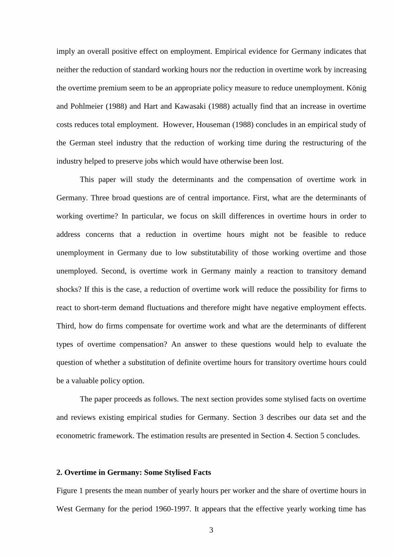
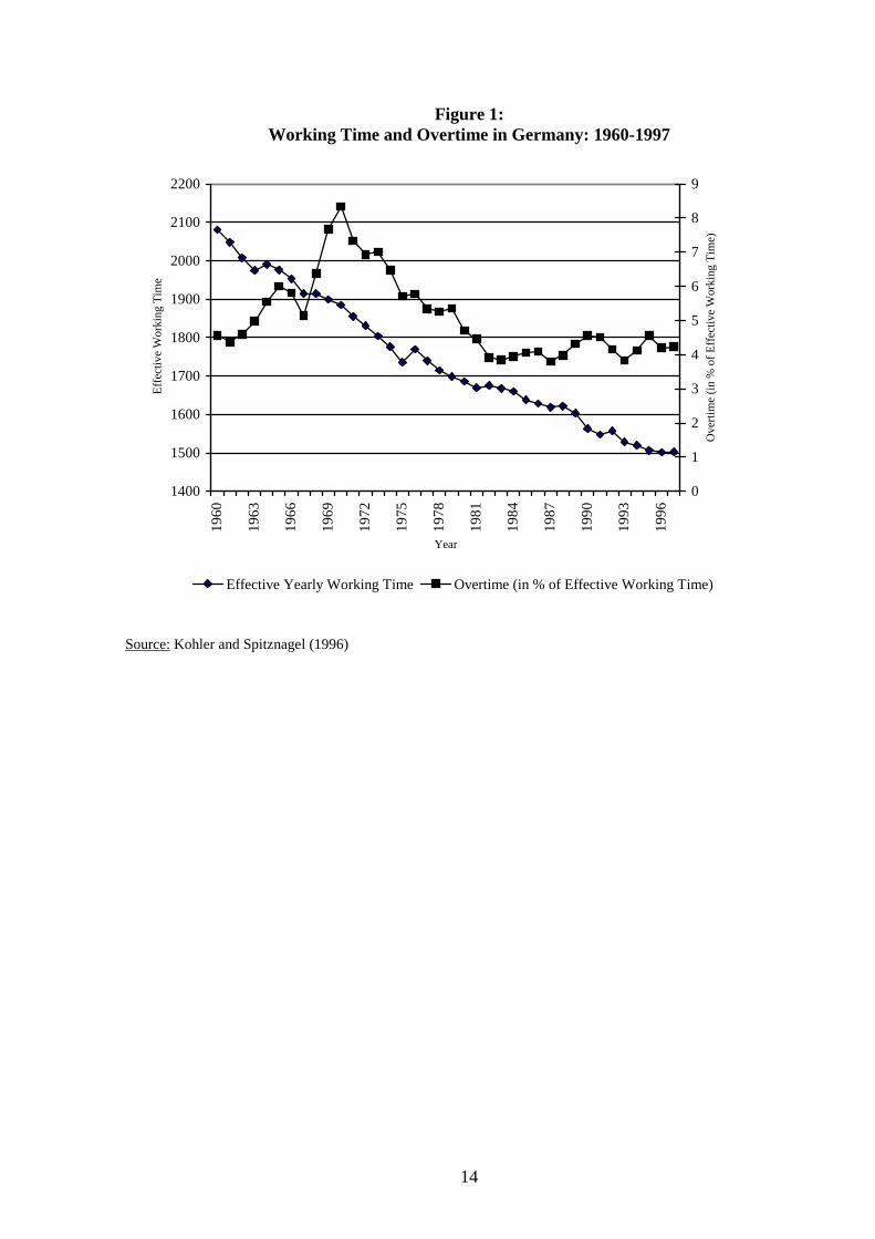
Figure 1 presents the mean number of yearly hours per worker and the share of overtime hours in
West Germany for the period 1960-1997. It appears that the effective yearly working time has
4
followed a strong downward trend from 2,081 yearly working hours in 1960 to 1,503 hours in
1997. This decline was shortly interrupted during the boom years of 1964, 1976 and 1992.
Compared to the effective working time, overtime work in Germany has followed a somewhat
different pattern. During the 1960's overtime hours increased in total as well as relative to
effective working time. It reached a peak in 1970 with 157 yearly hours of overtime per worker
(8.3% of the effective working time). Following the oil-crisis in the early 70's overtime work in
Germany decreased sharply to about 66 yearly overtime hours (4% of the effective working
time) in 1982. The share of overtime hours to total working time has remained relatively stable
around 4% since 1982. Among other reasons, the decline of overtime hours in Germany can be
explained by the rising importance of female and part-time workers, who traditionally work less
overtime, and an increased flexibility of working time schedules, which allow for intertemporal
substitution (Kohler and Spitznagel, 1996).
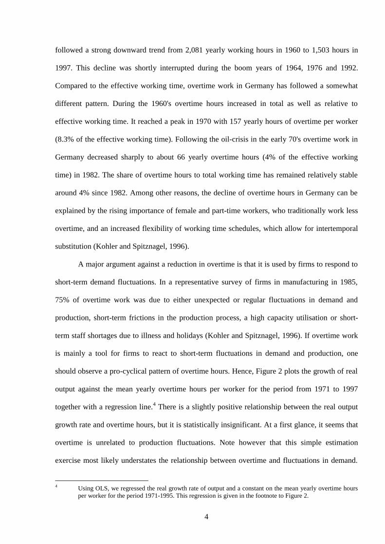
A major argument against a reduction in overtime is that it is used by firms to respond to
short-term demand fluctuations. In a representative survey of firms in manufacturing in 1985,
75% of overtime work was due to either unexpected or regular fluctuations in demand and
production, short-term frictions in the production process, a high capacity utilisation or short-
term staff shortages due to illness and holidays (Kohler and Spitznagel, 1996). If overtime work
is mainly a tool for firms to react to short-term fluctuations in demand and production, one
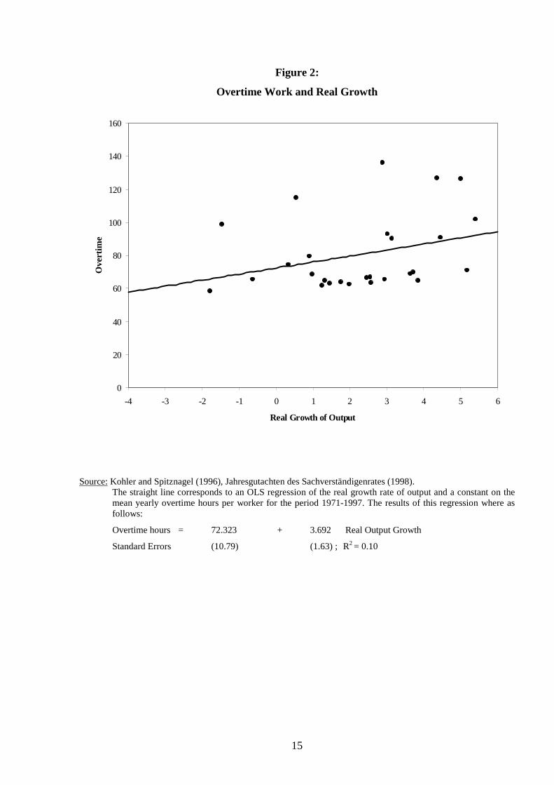
should observe a pro-cyclical pattern of overtime hours. Hence, Figure 2 plots the growth of real
output against the mean yearly overtime hours per worker for the period from 1971 to 1997
together with a regression line.4 There is a slightly positive relationship between the real output
growth rate and overtime hours, but it is statistically insignificant. At a first glance, it seems that
overtime is unrelated to production fluctuations. Note however that this simple estimation
exercise most likely understates the relationship between overtime and fluctuations in demand.
4 Using OLS, we regressed the real growth rate of output and a constant on the mean yearly overtime hours
per worker for the period 1971-1995. This regression is given in the footnote to Figure 2.
5
Among other reasons, overtime work due to seasonal fluctuations can not be captured by this
regression since it is based on yearly data and not separated according to industries. Furthermore,
there exists a bulk of empirical evidence (at least for the U.S.) that the demand for hours adjusts
much faster to demand shocks than the demand for employment (Hamermesh, 1993).
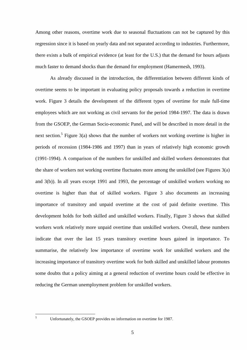
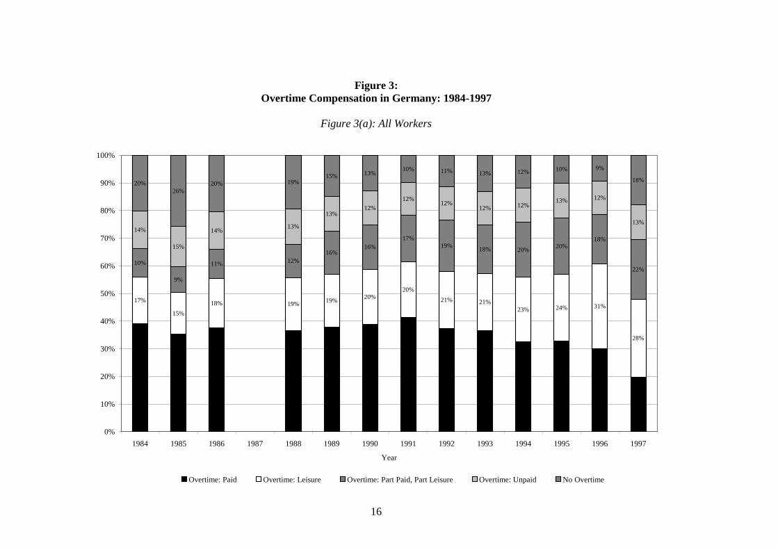
As already discussed in the introduction, the differentiation between different kinds of
overtime seems to be important in evaluating policy proposals towards a reduction in overtime
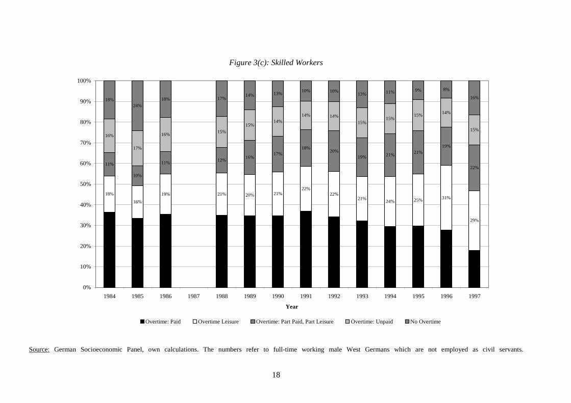
work. Figure 3 details the development of the different types of overtime for male full-time
employees which are not working as civil servants for the period 1984-1997. The data is drawn
from the GSOEP, the German Socio-economic Panel, and will be described in more detail in the
next section.5 Figure 3(a) shows that the number of workers not working overtime is higher in
periods of recession (1984-1986 and 1997) than in years of relatively high economic growth
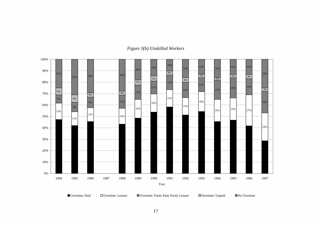
(1991-1994). A comparison of the numbers for unskilled and skilled workers demonstrates that
the share of workers not working overtime fluctuates more among the unskilled (see Figures 3(a)
and 3(b)). In all years except 1991 and 1993, the percentage of unskilled workers working no
overtime is higher than that of skilled workers. Figure 3 also documents an increasing
importance of transitory and unpaid overtime at the cost of paid definite overtime. This
development holds for both skilled and unskilled workers. Finally, Figure 3 shows that skilled
workers work relatively more unpaid overtime than unskilled workers. Overall, these numbers
indicate that over the last 15 years transitory overtime hours gained in importance. To
summarise, the relatively low importance of overtime work for unskilled workers and the
increasing importance of transitory overtime work for both skilled and unskilled labour promotes
some doubts that a policy aiming at a general reduction of overtime hours could be effective in
reducing the German unemployment problem for unskilled workers.
5 Unfortunately, the GSOEP provides no information on overtime for 1987.
6
3. Data and Econometric Methodology
For the empirical analysis of this paper we employ the German Socio-economic Panel (GSOEP),
a comprehensive panel of household and individual data for the period 1984-1997. Among other
socioeconomic characteristics, this data set provides rich information on issues such as wages,
education levels, occupational status, and employment history. For all years but 1987 the
GSOEP also includes detailed information on the working time of an individual, including the
contractual working time, overtime hours and the compensation of overtime hours. In our
empirical analysis we concentrate on full-time male West Germans who are not employed as
civil servants. After pooling all waves of the GSOEP and eliminating all observations with
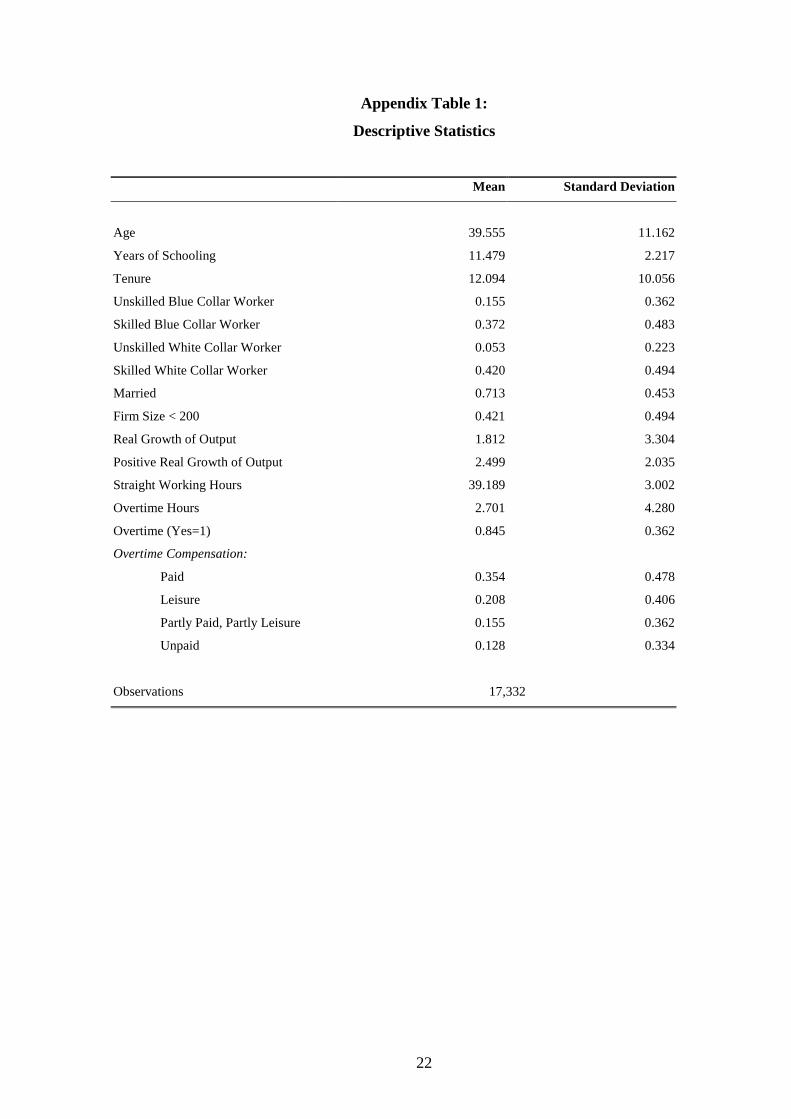
missing values we are left with a final sample of 17,332 individual observations.
Our empirical analysis consists of two steps. In the first step we examine the determinants
of actual overtime hours worked using a Tobit model which takes the form:
≤+>++
=0 ' if 0
0 ' if '
ii
iiiii X
XXY
εβεβεβ
(1)
where the dependent variable iY refers to the weekly overtime hours with respect to individual i,
iX is a vector of explanatory variables, β is a vector of coefficients, and iε is a normal
distributed error term with mean 0 and variance 2εσ .
In the second step we analyse the determinants of overtime compensation using a
multinomial logit model of the following form:
4, ..., 0,for )( Prob4
0
'
'
===∑
=
je
ejY
k
X
X
iik
ij
β
β
(2)
where 0=j if the individual had not worked overtime, 1=j if the individual had worked paid
definite overtime hours, 2=j if the individual had worked transitory overtime hours, 3=j if
the individual had been working partly paid overtime and partly transitory overtime, and 4=j if
the individual had worked unpaid overtime. iX refers to a vector of explanatory variables, jβ is
7
a vector of coefficients. In order to identify the parameters of the model, we impose the
normalisation 00 =β .
For the estimation exercise, we pooled single cross-sections of data for the period 1984-
1977 excluding 1987. In the pooled sample it is possible that the repeated observations of the
same individual are not independent of each other. To account for this problem we report robust
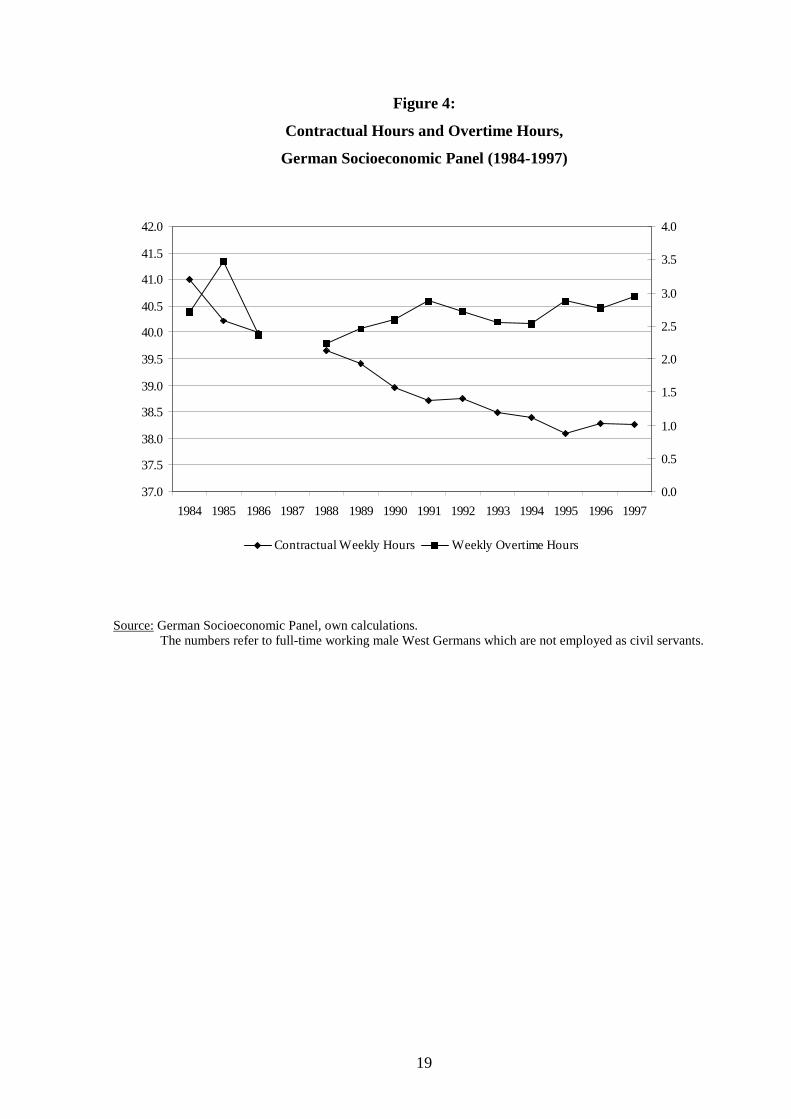
standard errors.6 Figure 4 exhibits the development of contractual weekly working hours and
overtime hours as they appear in our sample. Note that Figure 4 is very similar to the
development of working time based on aggregate data (see Figure 1). The mean contractual
weekly working time decreases from 41 hours in 1984 to 38 hours in 1997. Since 1987 weekly
overtime hours stay relatively stable around 2.5 hours. The development of overtime
compensation as it appears in our sample has already been discussed in the last section (see
Figure 3).
All our estimation equations include as explanatory variables the age and age squared of
the individual, his years of schooling and years of schooling squared, his tenure with the current
firm and tenure squared, contractual weekly hours, a time trend, a dummy variable which takes
the value of 1 if the individual is married and 0 otherwise, and a dummy variable which takes the
value of 1 if the individual is working in a firm with less than 200 employees and 0 otherwise.
To control for any business cycle effects of overtime we matched the data set on a yearly basis
with the real output growth rate for the industry a person is working in.7
To allow for asymmetries in the effect of the business cycle on overtime we further
include an interaction term between the real output growth rate and a dummy variable which
takes the value 1 if the real output growth rate is positive and 0 otherwise. Finally, we consider
6 The estimated variance is VMMV ˆ)]1/([ˆ * −= , where V̂ is the Huber-White sandwich estimator of the
variance and M the number of individuals in the pooled sample.7 In total we used data for 8 industries, including agriculture, mining, manufacturing, construction, trade,
services, the public sector and private households. The data for the real growth rate have been drawn fromSachverständigenrat (1998).
8
several dummy variables describing the occupational status of an individual, i.e. whether an
individual is employed as skilled blue collar worker, unskilled white collar worker, or skilled
white collar worker. Unskilled blue collar workers represent the reference group. Unskilled
workers are defined as employees who either need no, or only a short-term instruction, to
perform their job. Descriptive statistics for the variables used in the analysis are reported in
Table 1 of the Appendix.
4. Estimation Results
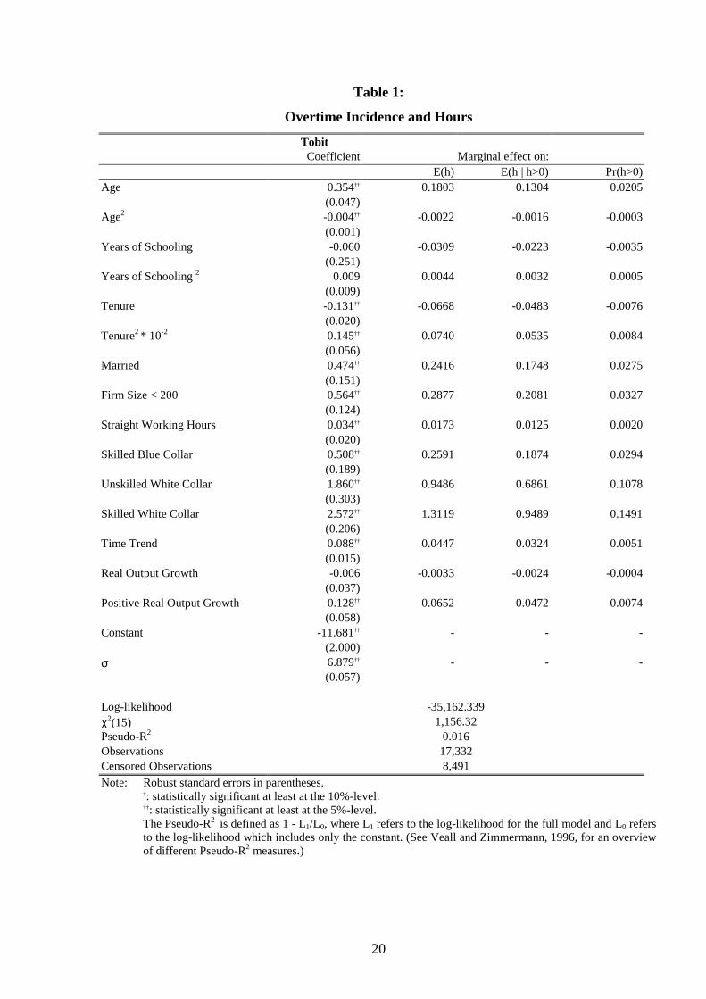
We first study the determinants of overtime incidence and hours, and then investigate the
different types of overtime compensation. The estimation results from the Tobit model are
contained in Table 1. The first column reports the estimated coefficients of the model, the second
column the estimated unconditional marginal effects on hours, the third column the estimated
marginal effects on hours conditional on the individual working overtime, and the last column
measures the marginal effect of each explanatory variable on the probability of overtime
incidence. All marginal effects are evaluated at the mean of the exogenous variables. For dummy
variables “marginal” also means a change in prediction caused by the discrete change of an
exogenous variable from 0 to 1.
The estimated coefficients for age exhibit an inverted U-shaped pattern, while the
parameters for years of schooling and firm tenure have a U-shaped structure. The effects of years
of schooling are statistically insignificant, however; individuals older than 44 work a diminishing
number of overtime hours; and tenure has a declining after 45 years. Married individuals and
individuals working in small firms have a higher probability of working overtime (2.8
percentage points for marriage and 3.3 percentage points for small firms), and they work a larger
numbers of hours. Marriage entails an overall increase of 8.9% in overtime hours, and a 5.4%
increase for those who already worked overtime. (Increases here and in the sequel are calculated
with reference to the sample mean level values.) Working for a small firm is associated with an
9
overall increase of 10.7% in overtime hours, and a 6.5% increase for those who already worked
overtime. These numbers indicate that a large part of the higher overtime hours in small firms is
due to a higher overtime incidence. The results are consistent with the existing evidence on
overtime incidence in the UK and the US.8
However, in contrast to evidence from the UK and the US, the number of contractual
weekly hours have a positive effect on the probability of overtime work and on overtime hours.
Since straight-time working hours have declined significantly over time in Germany, this implies
that overtime hours have also fallen through this interaction. The estimated coefficient suggests
that a decrease of one hour in normal working time per week causes a decline in the
unconditional overtime of about one minute. This is an important finding for policy: Firms have
not acted against the general working time reduction through an increase in overtime hours.
However, this effectively negative relationship works against the general time trend of increasing
overtime hours, as estimated by our model. The probability of working overtime, which is
slightly increasing over time, indicates an increased quasi-fixed costs of labour over the last 15
years.
It is clear that working overtime rises strictly with a worker’s level of qualification. White
collar workers have a higher probability of working overtime than blue collar workers, and
skilled workers have a higher probability of working overtime than unskilled workers. To be
more precise, in comparison with the reference group of unskilled blue collar workers, the
probability increases of working overtime are 2.9% (skilled blue), 10.8% (unskilled white) and
14.9% (skilled white). Skilled blue collar workers work 9.6% more overtime hours than the
unskilled workers from the same group. In comparison to the reference group, unskilled white
collar workers work 35% more overtime hours, and skilled white collar workers as many as 49%
more overtime hours.
8 See Bell and Hart (1998b, 1999) for the UK and Trejo (1991, 1993) for the US.
10
A common argument is that overtime work is used by firms as an instrument to react to
business cycle fluctuations. To examine this hypothesis we include real output growth rates at
the industry levels and allow for asymmetric reactions. We find a significant effect only for
periods of positive output growth. An increase of the output growth of 1 percentage point in a
boom period leads to an overall increase of overtime hours of 2.4% which could be separated
into an increase in the probability to work overtime of 0.7% and an increase of overtime hours
conditional on working overtime of 1.7%. Hence, in boom periods firms mainly change the
amount of overtime hours to meet demand fluctuations.
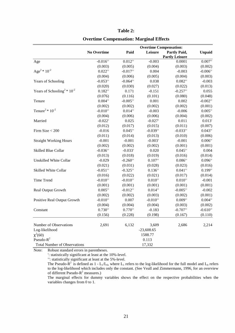
More light can be shed on the motives behind overtime working by a joint investigation
of the alternatives “no overtime”, and the different forms of overtime compensation, namely
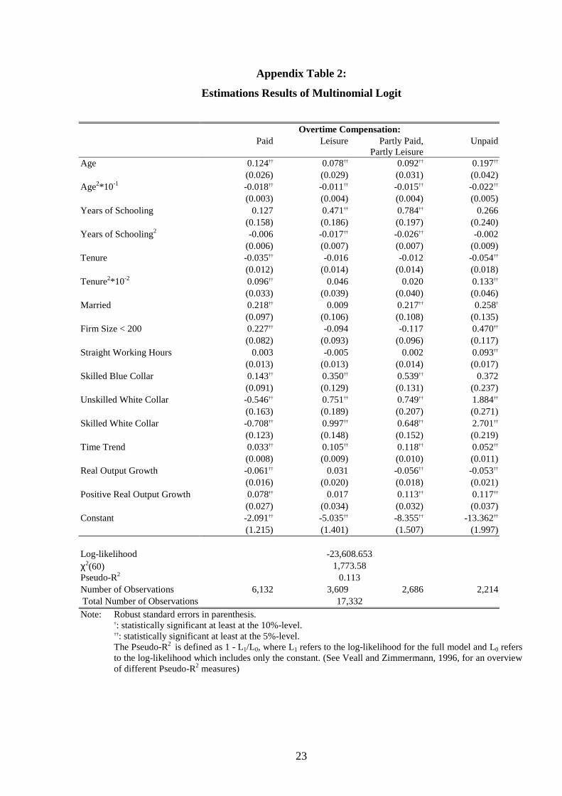
“paid”, “leisure”, “partly paid, partly leisure”, and “unpaid”. The estimated coefficients of the
employed multinomial logit model are reported in Appendix Table 2. These parameter estimates
are again used to calculate marginal effects for the probabilities, and these are provided in Table
2. As before, “marginal” in case of a dummy variable means that the value changes from 0 to 1.
Note that a series of Hausman tests suggest that none of the 5 alternatives are irrelevant.
As we had seen before, the likelihood of working overtime is rising with age according to
an inverted U-shaped pattern. Table 2 now shows that this rise is in paid and unpaid overtime.
Schooling has again an inverted U-shaped effect on working overtime, but this works basically
against paid work. Tenure has statistically significant U-shaped structures for the incidence of
overtime work as well as for paid and unpaid overtime work. In general, married people work
more overtime, but are less likely be compensated by leisure. Small firms require more paid and
unpaid overtime work, but compensate less with leisure. This result suggests that small firms
rely relatively more on definite overtime instead of using transitory overtime indicating that
small firms may face higher problems in introducing flexible working time schedules. Straight
working hours increase the likelihood of unpaid overtime work significantly and has a
marginally significant negative effect on the probability to be compensated with leisure.
11
Skill levels play an important role. According to the multinomial logit model in Table 2,
skilled blue collar workers have a 3.6% higher probability to work overtime than unskilled blue
collar workers; this is largely the result of more work compensated by either payments or leisure.
However, skilled blue collar workers have a lower probability to work solely paid overtime
hours than unskilled blue collar workers. This qualitative pattern is very consistent for higher
skill levels, namely for unskilled and skilled white collar workers. Marginal effects are larger in
absolute terms, the higher the skill level is. In comparison to an unskilled blue collar worker, a
skilled white collar worker has a 5.1% larger probability of working overtime: This separates
into a 33% reduction in paid overtime work, and an increase of 13.6% in leisure, a 19.9%
increase in unpaid work and a 4.1% increase in the category “partly paid, partly leisure”. Hence,
overtime work matters for the high-skilled; but they work largely unpaid or transitory overtime.
Finally, as Table 2 shows us, there is an increase in overtime work measured by the time
trend coefficient. This result is explained by an increase in the categories “leisure” and “partly
paid, partly leisure”, while the likelihood of paid overtime work is declining over time. This
result suggests a rising importance of working time accounts. The overall role of real output
growth is asymmetric: the incidence of overtime work reacts counter-cyclical in periods of
negative growth and pro-cyclical in periods of positive growth. Paid overtime work reacts
counter-cyclical and is symmetric. Transitory overtime reacts pro-cyclical to economic growth
with a lower effect in periods of positive output growth. Finally, real output growth has
significant positive effects on unpaid overtime and the category “partly paid, partly leisure” in
periods of positive output growth. These results indicate that firms react to demand fluctuations
mainly by redistributing working time instead of increasing definite overtime. This also implies
that if output growth is positive in the long-run, there is a persistent decline in paid overtime in
favour of transitory overtime or unpaid overtime.
12
5. Conclusions
Reducing overtime work has been largely advocated as an effective instrument to fight
unemployment. On the basis of the findings of this study, we argue that such a strategy may have
some problems. Unemployment is largely a problem of the unskilled. However, low-skilled
people work less overtime. To be more concrete, one of our estimates demonstrates that in
comparison to unskilled blue collar workers, skilled white collar workers have as many as 49%
more overtime hours, holding all other measured factors constant. A skilled white collar worker
faces a 5.1% larger probability of working overtime, but this made up of a 33% reduction in paid
work, a 13.6% increase in leisure, a 19.9% increase in unpaid work and a 4.1% increase in the
category “partly paid, partly leisure”.
Hence, overtime work is largely a matter for the high-skilled; but they work largely
unpaid overtime or are compensated by leisure. Reducing overtime work across all groups would
cause a labour shortage among the skilled workers. If skilled and unskilled workers are
complements in production, this would also cause a decline in the demand for the unskilled, and
hence further problems in this market segment. Overtime work for unskilled blue collar workers
is largely paid work. It would make more sense to establish a condition of not financially
compensating overtime work for unskilled workers.
Paid overtime work is in decline anyway. There is some indication that overtime work is
used to adjust to boom phases of the economy. But it is also clear that positive growth rates of
sectoral output induce a decline in paid overtime in favour of leisure compensation. Hence, a
strategy of reducing paid overtime becomes less and less relevant anyway.
13
References
Bell, D. N. F., and R. A. Hart (1998a): "Working Time in Great Britain, 1975-1994: Evidencefrom the New Earnings Panel Data," Journal of the Royal Statistical Society (Series A),161, 327-348.
Bell, D. N. F., and R. A. Hart (1998b): "Unpaid Work," forthcoming in Economica.Bell, D. N. F., and R. A. Hart (1999): "Overtime Working in an Unregulated Labour Market,"
IZA Discussion Paper No. 44 , Bonn.Calmfors, L. and M. Hoel (1988): "Work Sharing and Overtime," Scandinavian Journal of
Economics, 90(1), 45-52.Ehrenberg, R. G. (1971): Fringe Benefits and Overtime Behavior. Lexington, Mass.: D.C. Heath.Ehrenberg, R. G. and P. Schumann (1982): Longer Hours or More Jobs? Ithaca, NY: Cornell
University Press.Gerlach, K., and O. Hübler (1987): "Personalnebenkosten, Beschäftigung und Arbeitsstunden
aus neoklassischer und institutioneller Sicht," in: F. Buttler, K. Gerlach, and R. Scheide(eds.): Arbeitsmarkt und Beschäftigung. Frankfurt: Campus, 291-331.
Hamermesh, D. C. (1993): Labor Demand. Princeton, NJ: Princeton University Press.Hart, R. A. (ed.) (1988): Employment, Unemployment and Labor Utilization. Boston, Mass.:
Unwin Hyman.Hart, R. A. and S. Kawasaki (1988): "Payroll Taxes and Factor Demand," Research in Labor
Economics, 9, 257-285.Hart, R. A. and R. J. Ruffell (1993): "The Cost of Overtime Working in British Production
Industries," Economica, 60, 183-201.Houseman, S. N. (1988): "Shorter Working Time and Job Security: Labor Adjustment in the
Steel Industry," in R. A. Hart (ed.): Employment, Unemployment and Labor Utilization.Boston, Mass.: Unwin Hyman, 64-85.
Kohler, H. and E. Spitznagel: "Überstunden in Deutschland: Eine empirische Analyse," IABWerkstattbericht, No. 4.
König. H. and W. Pohlmeier (1988): "Employment, Labour Utilization and Procyclical LabourDemand," Kyklos, 41, 551-572.
Sachverständigenrat zur Begutachtung der gesamtwirtschaftlichen Entwicklung (1998): Vorweitreichenden Entscheidungen. Jahresgutachten 1998/99. Stuttgart: Metzler-Poeschel.
Trejo, S. J. (1991): "Compensating Differentials and Overtime Pay Regulations," AmericanEconomic Review, 81, 719-770.
Trejo, S. J. (1993) "Overtime Pay, Overtime Hours, and Labour Unions," Journal of LaborEconomics, 11, 253-278.
Veall, M. R. and K. F. Zimmermann (1996): “Pseudo-R2 Measures for Some Limited DependentVariable Models,” Journal of Economic Surveys, 10, 241-259.
14
Figure 1:Working Time and Overtime in Germany: 1960-1997
Source: Kohler and Spitznagel (1996)
1400
1500
1600
1700
1800
1900
2000
2100
2200
19
60
19
63
19
66
19
69
19
72
19
75
19
78
19
81
19
84
19
87
19
90
19
93
19
96
Year
Effe
ctiv
e W
orki
ng T
ime
0
1
2
3
4
5
6
7
8
9
Ove
rtim
e (in
% o
f Effe
ctiv
e W
orki
ng T
ime)
Effective Yearly Working Time Overtime (in % of Effective Working Time)
15
Figure 2:
Overtime Work and Real Growth
Source: Kohler and Spitznagel (1996), Jahresgutachten des Sachverständigenrates (1998).The straight line corresponds to an OLS regression of the real growth rate of output and a constant on themean yearly overtime hours per worker for the period 1971-1997. The results of this regression where asfollows:
Overtime hours = 72.323 + 3.692 Real Output Growth
Standard Errors (10.79) (1.63) ; R2 = 0.10
0
20
40
60
80
100
120
140
160
-4 -3 -2 -1 0 1 2 3 4 5 6
Real Growth of Output
Ove
rtim
e
16
Figure 3:Overtime Compensation in Germany: 1984-1997
Source: German Socioeconomic Panel, own calculations. The numbers refer to full-time working male West Germans which are not employed as civil servants.
Overtime: Paid Overtime Leisure Overtime: Part Paid, Part Leisure Overtime: Unpaid No Overtime
19
Figure 4:
Contractual Hours and Overtime Hours,
German Socioeconomic Panel (1984-1997)
Source: German Socioeconomic Panel, own calculations.The numbers refer to full-time working male West Germans which are not employed as civil servants.
Note: Robust standard errors in parentheses.†: statistically significant at least at the 10%-level.††: statistically significant at least at the 5%-level.The Pseudo-R2 is defined as 1 - L1/L0, where L1 refers to the log-likelihood for the full model and L0 refersto the log-likelihood which includes only the constant. (See Veall and Zimmermann, 1996, for an overviewof different Pseudo-R2 measures.)
Number of Observations 2,691 6,132 3,609 2,686 2,214Log-likelihood -23,608.65χ2(60) 1588.77Pseudo-R2 0.113Total Number of Observations 17,332
Note: Robust standard errors in parentheses.†: statistically significant at least at the 10%-level.††: statistically significant at least at the 5%-level.The Pseudo-R2 is defined as 1 - L1/L0, where L1 refers to the log-likelihood for the full model and L0 refersto the log-likelihood which includes only the constant. (See Veall and Zimmermann, 1996, for an overviewof different Pseudo-R2 measures.)The marginal effects for dummy variables shows the effect on the respective probabilities when thevariables changes from 0 to 1.
Log-likelihood -23,608.653χ2(60) 1,773.58Pseudo-R2 0.113Number of Observations 6,132 3,609 2,686 2,214Total Number of Observations 17,332
Note: Robust standard errors in parenthesis.†: statistically significant at least at the 10%-level.††: statistically significant at least at the 5%-level.The Pseudo-R2 is defined as 1 - L1/L0, where L1 refers to the log-likelihood for the full model and L0 refersto the log-likelihood which includes only the constant. (See Veall and Zimmermann, 1996, for an overviewof different Pseudo-R2 measures)