J. Fluid Mech. (2015), vol. 779, pp. 371–389. c Cambridge University Press 2015 doi:10.1017/jfm.2015.273 371 Turbulent boundary layer statistics at very high Reynolds number M. Vallikivi 1 , M. Hultmark 1, † and A. J. Smits 1, 2 1 Department of Mechanical and Aerospace Engineering, Princeton University, Princeton, NJ 08544, USA 2 Department of Mechanical and Aerospace Engineering, Monash University, Melbourne, VIC 3800, Australia (Received 10 June 2014; revised 14 January 2015; accepted 7 May 2015; first published online 17 August 2015) Measurements are presented in zero-pressure-gradient, flat-plate, turbulent boundary layers for Reynolds numbers ranging from Re τ = 2600 to Re τ = 72 500 (Re θ = 8400–235 000). The wind tunnel facility uses pressurized air as the working fluid, and in combination with MEMS-based sensors to resolve the small scales of motion allows for a unique investigation of boundary layer flow at very high Reynolds numbers. The data include mean velocities, streamwise turbulence variances, and moments up to 10th order. The results are compared to previously reported high Reynolds number pipe flow data. For Re τ > 20 000, both flows display a logarithmic region in the profiles of the mean velocity and all even moments, suggesting the emergence of a universal behaviour in the statistics at these high Reynolds numbers. Key words: turbulent boundary layers, turbulent flows 1. Introduction The scaling of turbulent wall-bounded flows with Reynolds number has been the subject of much recent interest and debate (Marusic et al. 2010; Smits, McKeon & Marusic 2011a; Smits & Marusic 2013), and new experiments have expanded considerably the range of Reynolds numbers available for study. For example, examinations of pipe flow have reported mean flow data at values of Re τ as high as 530 000 (Zagarola & Smits 1998; McKeon et al. 2004), where Re τ is the friction Reynolds number, with turbulence data at values up to 98000 (Hultmark et al. 2012, 2013; Rosenberg et al. 2013). For boundary layer flows under laboratory conditions, the corresponding values are 70 000 (Winter & Gaudet 1973) and 19 000 (Mathis, Hutchins & Marusic 2009), although some limited but valuable turbulence data were acquired at 69 000 in the LCC facility by Winkel et al. (2012), and at 650 000 in the neutral atmospheric boundary layer by Hutchins et al. (2012). The available laboratory data are limited in Reynolds number primarily because of experimental difficulties. Conducting high Reynolds number experiments usually requires large and often expensive facilities, and for scaling studies the flows need to be of high quality and employ high-resolution instrumentation. Here, we use a pressurized facility, the Princeton High Reynolds Number Test Facility (HRTF), to † Email address for correspondence: [email protected]
Turbulent boundary layer statistics at very highReynolds number
M. Vallikivi1, M. Hultmark1,† and A. J. Smits1,2
1Department of Mechanical and Aerospace Engineering, Princeton University, Princeton, NJ 08544, USA2Department of Mechanical and Aerospace Engineering, Monash University, Melbourne,
VIC 3800, Australia
(Received 10 June 2014; revised 14 January 2015; accepted 7 May 2015;first published online 17 August 2015)
Measurements are presented in zero-pressure-gradient, flat-plate, turbulent boundarylayers for Reynolds numbers ranging from Reτ = 2600 to Reτ = 72 500 (Reθ =8400–235 000). The wind tunnel facility uses pressurized air as the working fluid,and in combination with MEMS-based sensors to resolve the small scales of motionallows for a unique investigation of boundary layer flow at very high Reynoldsnumbers. The data include mean velocities, streamwise turbulence variances, andmoments up to 10th order. The results are compared to previously reported highReynolds number pipe flow data. For Reτ > 20 000, both flows display a logarithmicregion in the profiles of the mean velocity and all even moments, suggesting theemergence of a universal behaviour in the statistics at these high Reynolds numbers.
1. IntroductionThe scaling of turbulent wall-bounded flows with Reynolds number has been the
subject of much recent interest and debate (Marusic et al. 2010; Smits, McKeon& Marusic 2011a; Smits & Marusic 2013), and new experiments have expandedconsiderably the range of Reynolds numbers available for study. For example,examinations of pipe flow have reported mean flow data at values of Reτ as highas 530 000 (Zagarola & Smits 1998; McKeon et al. 2004), where Reτ is the frictionReynolds number, with turbulence data at values up to 98 000 (Hultmark et al. 2012,2013; Rosenberg et al. 2013). For boundary layer flows under laboratory conditions,the corresponding values are 70 000 (Winter & Gaudet 1973) and 19 000 (Mathis,Hutchins & Marusic 2009), although some limited but valuable turbulence data wereacquired at 69 000 in the LCC facility by Winkel et al. (2012), and at 650 000 in theneutral atmospheric boundary layer by Hutchins et al. (2012).
The available laboratory data are limited in Reynolds number primarily becauseof experimental difficulties. Conducting high Reynolds number experiments usuallyrequires large and often expensive facilities, and for scaling studies the flows needto be of high quality and employ high-resolution instrumentation. Here, we use apressurized facility, the Princeton High Reynolds Number Test Facility (HRTF), to
generate very high Reynolds number flat-plate boundary layers. We report resultsobtained at a maximum Reynolds number based on the momentum thickness of235 000, which is believed to be higher than that investigated in any previouslaboratory study featuring well-controlled initial and boundary conditions. The HRTFis the counterpart to the Princeton Superpipe facility, which has been extensively usedto examine very high Reynolds number pipe flows. Here, we present the first datafrom this unique boundary layer wind tunnel, which, together with novel nanoscaleflow sensors, will enable us to investigate canonical flat-plate boundary layers overan unprecedented range of Reynolds numbers.
The friction Reynolds number, Reτ = uτδ/ν, provides a common standard forcomparisons among wall-bounded flows. Here, uτ =√τw/ρ is the friction velocity, τw
is the wall shear stress, ρ and ν are fluid density and kinematic viscosity, respectively,and δ is the boundary layer thickness δ99, or the pipe radius R, or the half-heightof the channel h. This Reynolds number, also known as the von Kármán number,characterizes the range of scales present in the flow, and avoids the use of morespecific velocity and length scales such as the free-stream velocity U∞, the bulkvelocity 〈U〉, the momentum thickness θ , or the displacement thickness δ∗.
For turbulent wall-bounded flows at sufficiently large Reynolds numbers, we expectthat for y+ = yuτ/ν � 1 and y/δ � 1, the mean velocity U behaves logarithmicallyaccording to
U+ = 1κ
ln y+ + B (1.1)
(Millikan 1938), where U+=U/uτ , y is the wall-normal distance, κ is the von Kármánconstant, and B is the additive constant for the mean velocity. The values of κ reportedin the past have varied over a considerable range, with values as low as 0.38 in aboundary layer (Österlund et al. 2000) and as high as 0.42 in a pipe (McKeon et al.2004). A recent study by Bailey et al. (2014) showed that for pipe flow κ = 0.40±0.02, where the uncertainty estimate reflects the many sources of error that make itdifficult to find κ more precisely even when the friction velocity is well known. Forboundary layers one would expect an even larger variation due to the difficulty inestimating uτ .
The pipe flow measurements by Zagarola & Smits (1998) and McKeon et al. (2004)revealed that the start of the log-law region in the mean flow, commonly assumed tobe located at y+ = 30–50, was actually located much further from the wall at y+ =600, or even y+= 1000. In boundary layers, George & Castillo (1997) argued that theinner limit was located at y+≈ 300, whereas Wei et al. (2005) suggested a Reynolds-number-dependent lower limit and Nagib, Chauhan & Monkewitz (2007) reported avalue of y+= 200. As to the outer limit, values in the literature range from y/δ= 0.08to 0.3, with Marusic et al. (2013) suggesting a value of 0.15. With an inner limit ofy+ = 300, and an outer limit of y/δ = 0.15, a decade of logarithmic variation in themean velocity of a boundary layer is not expected to occur until Reτ = 20 000, whichis the upper limit of the detailed data sets that have so far been available for boundarylayers.
As to the behaviour of the turbulence, Townsend (1976) and Perry, Henbest &Chong (1986) suggested that a logarithmic behaviour in streamwise and wall-parallelfluctuations should also occur in the region where (1.1) holds, if the Reynolds numberis large enough. That is, for the streamwise velocity fluctuations u, we would expect
u2+ = B1 − A1 lnyδ, (1.2)
Turbulent boundary layer statistics at very high Reynolds number 373
where u2+= u2/u2τ , A1 is the Townsend–Perry constant, and B1 is the additive constant
for the variance. This logarithmic behaviour was first observed experimentally in pipeflow over a significant wall-normal extent by Hultmark et al. (2012), where it onlybecame evident for y/R< 0.12 once Reτ > 20 000, with a spatial extent that increasedwith Reynolds number. Marusic et al. (2013) suggested that this scaling also appliesin boundary layers, and proposed a universal value of A1 = 1.26.
In deriving (1.2), Townsend appealed to his attached eddy hypothesis, where theturbulent eddy length scales are assumed to be proportional to y with a populationdensity proportional to y−1. Meneveau & Marusic (2013) used this hypothesis to showthat if the summands are assumed to be statistically independent (as in the case ofnon-interacting eddies), the pth root of moments of velocity fluctuations is expectedto behave according to
〈(u+)2p〉1/p = Bp − Ap lnyδ, (1.3)
where Ap and Bp are constants, at least at fixed Reynolds number. They examined thevalidity of this generalized logarithmic law in boundary layers with Reτ up to 19 000,and found that the behaviour of high-order moments was sub-Gaussian, and that theremay be a universal value of Ap.
It is evident from this previous work that high Reynolds number data revealintriguing trends in the scaling of the mean flow and the turbulence. At the sametime it is clear that for boundary layers high-quality turbulence data over anyextensive range of Reynolds numbers is limited to values of Reτ < 20 000, andit appears that this might be the lower limit of what is possibly the start of anasymptotic behaviour (Smits & Marusic 2013). In order to extend the boundarylayer observations beyond this value, we now describe a new experimental study thatexamines turbulent boundary layer behaviour for 26006Reτ 6 72 500. Here, we focuson the behaviour of the mean flow, the variance, and the higher-order moments ofthe streamwise velocity fluctuations. The spectral behaviour is reported separately byVallikivi, Ganapathisubramani & Smits (2015). We will, wherever possible, comparethe boundary layer data with the results of pipe flow at similar Reynolds numbers.
2. Experimental methodsThe measurements were conducted in the HRTF at the Princeton University Gas
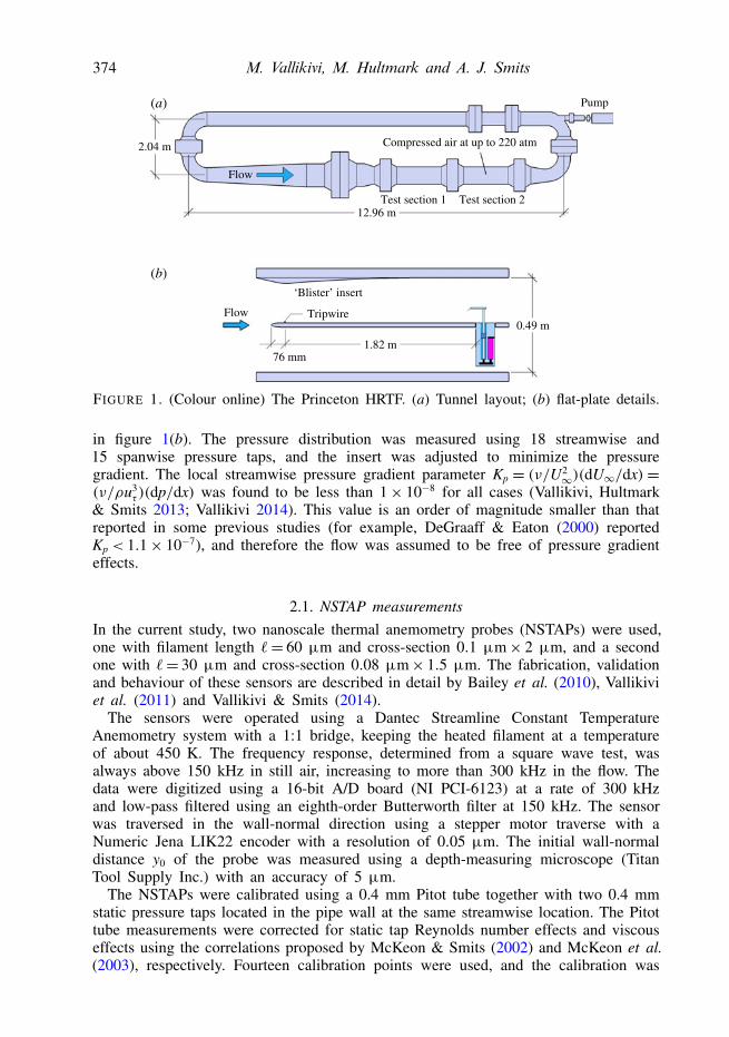
Dynamics Laboratory. The HRTF is a closed-loop wind tunnel that uses air atpressures up to 220 atm as the working fluid. The tunnel has a maximum speed of12 m s−1 and free-stream turbulence intensity levels between 0.3 and 0.6 %. It hastwo working sections, each 2.44 m long with a 0.49 m inner diameter, as shown infigure 1(a). The facility is described in further detail by Jiménez, Hultmark & Smits(2010).
A 2.06 m flat-plate model with an elliptic leading edge was mounted in thedownstream test section of the wind tunnel. A 1 mm square tripwire, located 76 mmfrom the leading edge, was used to trip the boundary layer. A single measurementstation was used, located 1.82 m downstream of the tripwire (figure 1b). Thealuminum surface of the plate was polished to a mirror finish. The surface roughnesswas estimated using an optical microscope and comparator plates and found to be lessthan 0.15 µm, corresponding to k+rms < 0.4 at the highest Reynolds number studied,so that for all conditions the plate was assumed to be hydraulically smooth.
The pressure distribution in the circular test section was adjusted using a ‘blister’insert attached to the tunnel wall on the opposite side of the plate, as shown
in figure 1(b). The pressure distribution was measured using 18 streamwise and15 spanwise pressure taps, and the insert was adjusted to minimize the pressuregradient. The local streamwise pressure gradient parameter Kp = (ν/U2
∞)(dU∞/dx)=(ν/ρu3
τ )(dp/dx) was found to be less than 1× 10⁻⁸ for all cases (Vallikivi, Hultmark& Smits 2013; Vallikivi 2014). This value is an order of magnitude smaller than thatreported in some previous studies (for example, DeGraaff & Eaton (2000) reportedKp < 1.1× 10⁻⁷), and therefore the flow was assumed to be free of pressure gradienteffects.
2.1. NSTAP measurementsIn the current study, two nanoscale thermal anemometry probes (NSTAPs) were used,one with filament length `= 60 µm and cross-section 0.1 µm× 2 µm, and a secondone with `= 30 µm and cross-section 0.08 µm× 1.5 µm. The fabrication, validationand behaviour of these sensors are described in detail by Bailey et al. (2010), Vallikiviet al. (2011) and Vallikivi & Smits (2014).
The sensors were operated using a Dantec Streamline Constant TemperatureAnemometry system with a 1:1 bridge, keeping the heated filament at a temperatureof about 450 K. The frequency response, determined from a square wave test, wasalways above 150 kHz in still air, increasing to more than 300 kHz in the flow. Thedata were digitized using a 16-bit A/D board (NI PCI-6123) at a rate of 300 kHzand low-pass filtered using an eighth-order Butterworth filter at 150 kHz. The sensorwas traversed in the wall-normal direction using a stepper motor traverse with aNumeric Jena LIK22 encoder with a resolution of 0.05 µm. The initial wall-normaldistance y0 of the probe was measured using a depth-measuring microscope (TitanTool Supply Inc.) with an accuracy of 5 µm.
The NSTAPs were calibrated using a 0.4 mm Pitot tube together with two 0.4 mmstatic pressure taps located in the pipe wall at the same streamwise location. The Pitottube measurements were corrected for static tap Reynolds number effects and viscouseffects using the correlations proposed by McKeon & Smits (2002) and McKeon et al.(2003), respectively. Fourteen calibration points were used, and the calibration was
Turbulent boundary layer statistics at very high Reynolds number 375
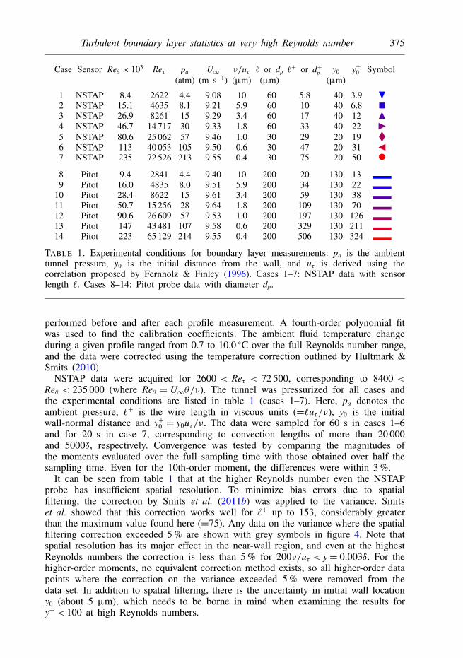
TABLE 1. Experimental conditions for boundary layer measurements: pa is the ambienttunnel pressure, y0 is the initial distance from the wall, and uτ is derived using thecorrelation proposed by Fernholz & Finley (1996). Cases 1–7: NSTAP data with sensorlength `. Cases 8–14: Pitot probe data with diameter dp.
performed before and after each profile measurement. A fourth-order polynomial fitwas used to find the calibration coefficients. The ambient fluid temperature changeduring a given profile ranged from 0.7 to 10.0 ◦C over the full Reynolds number range,and the data were corrected using the temperature correction outlined by Hultmark &Smits (2010).
NSTAP data were acquired for 2600 < Reτ < 72 500, corresponding to 8400 <Reθ < 235 000 (where Reθ = U∞θ/ν). The tunnel was pressurized for all cases andthe experimental conditions are listed in table 1 (cases 1–7). Here, pa denotes theambient pressure, `+ is the wire length in viscous units (=`uτ/ν), y0 is the initialwall-normal distance and y+0 = y0uτ/ν. The data were sampled for 60 s in cases 1–6and for 20 s in case 7, corresponding to convection lengths of more than 20 000and 5000δ, respectively. Convergence was tested by comparing the magnitudes ofthe moments evaluated over the full sampling time with those obtained over half thesampling time. Even for the 10th-order moment, the differences were within 3 %.
It can be seen from table 1 that at the higher Reynolds number even the NSTAPprobe has insufficient spatial resolution. To minimize bias errors due to spatialfiltering, the correction by Smits et al. (2011b) was applied to the variance. Smitset al. showed that this correction works well for `+ up to 153, considerably greaterthan the maximum value found here (=75). Any data on the variance where the spatialfiltering correction exceeded 5 % are shown with grey symbols in figure 4. Note thatspatial resolution has its major effect in the near-wall region, and even at the highestReynolds numbers the correction is less than 5 % for 200ν/uτ < y= 0.003δ. For thehigher-order moments, no equivalent correction method exists, so all higher-order datapoints where the correction on the variance exceeded 5 % were removed from thedata set. In addition to spatial filtering, there is the uncertainty in initial wall locationy0 (about 5 µm), which needs to be borne in mind when examining the results fory+ < 100 at high Reynolds numbers.
376 M. Vallikivi, M. Hultmark and A. J. Smits
1
2
3
4
5
103 104 105
FIGURE 2. Boundary layer skin friction coefficient Cf :E, Preston tube;@, Clauser fit forPitot data sets;p, Clauser fit for NSTAP data sets (Clauser 1956); ∗, DeGraaff & Eaton(2000); solid line, Fernholz & Finley (1996); dashed line, Winter & Gaudet (1973). Errorbars indicate ±5 %.
2.2. Pitot tube measurementsIn addition to the NSTAP data, Pitot tube measurements were taken for 2800 <Reτ < 65 000, corresponding to 9400<Reθ < 223 000. The experimental conditions forthese cases are given in table 1 (cases 8–14). A Pitot probe with an outer diameterof dp = 0.20 mm was used, in conjunction with two 0.4 mm static pressure taps inthe plate. The pressure difference was measured using a DP15 Validyne pressuretransducer with a 1.40 kPa range which was calibrated against a manometer standard.As for the NSTAP measurements, the initial wall distance of the Pitot probe y0 wasmeasured using a depth-measuring optical microscope and the probe was traversed inthe wall-normal direction using a stepper motor traverse with a resolution of 0.05 µm.The Pitot tube measurements were corrected following Bailey et al. (2013), includingthe static tap correction by McKeon et al. (2003), viscous and shear corrections byZagarola & Smits (1998), and the near-wall correction by MacMillan (1957). The datafor wall distances smaller than 2dp were neglected, as in the pipe flow experimentsdescribed by Bailey et al. (2014). Further details on the experimental techniques aregiven by Vallikivi (2014).
2.3. Friction velocity
To determine uτ and the skin friction coefficient Cf = 2u2τ/U
2∞, a number of different
methods were used. First, the 0.2 mm Pitot probe when in contact with the wallwas used as a Preston tube (Patel 1965; Zagarola, Williams & Smits 2001). Second,the Clauser chart technique (Clauser 1956) was used, where the log-law was fittedto the velocity profiles using the constants κ = 0.40 and B = 5.1 recommended byColes (1956). These results were compared to the skin friction correlation proposedby Fernholz & Finley (1996), as well as data from one of the few direct measurementsof skin friction using a drag plate at high Reynolds number (Winter & Gaudet 1973)(see figure 2). For comparison, values from DeGraaff & Eaton (2000) found using theClauser chart are also shown.
All Cf estimates except for the Preston tube data had a standard deviation less than3 % compared to the Fernholz correlation. In addition, the Fernholz correlation closely
Turbulent boundary layer statistics at very high Reynolds number 377
Case ReD Reτ pa (atm) 〈U〉 (m s−1) ν/uτ (µm) ` (µm) `+ y0 (µm) y+0 Symbol
TABLE 2. Pipe flow data for comparison, from Hultmark et al. (2013).
matches the average value obtained by the other methods, and it agrees well with theforce plate measurements by Winter & Gaudet (1973) over the same Reynolds numberrange. Hence, we used the value of uτ determined from the Fernholz correlation forall subsequent data analysis.
2.4. Pipe flow data for comparisonWe compare the turbulent boundary layer data with that from fully developed turbulentpipe flow obtained by Hultmark et al. (2012, 2013). The cases used for comparisonare listed in table 2, and cover 3300 6 Reτ 6 98 000.
3. Results and discussionIn presenting the results, we use a single notation δ to denote the outer length scale,
that is, the boundary layer thickness for boundary layer data and the pipe radius forpipe flow data.
3.1. Mean flowThe mean velocity profiles for the boundary layer are shown in figure 3. Theagreement between the NSTAP and Pitot profiles is within 1.3 %, well within theuncertainty on U (estimated to be <2.2 %). The mean velocity behaviour and scalingin boundary layers may be compared to the behaviour in pipe flow by referring tothe extensive discussions of pipe flows given by Zagarola & Smits (1998), McKeonet al. (2004), Hultmark et al. (2013) and Bailey et al. (2014), and so this will not berepeated here. Suffice it to say that both flows show an extended region of logarithmicbehaviour, although for the boundary layer this behaviour starts closer to the wallcompared to pipe flows, where the log-law only appears for y+ > 600–800. Themiddle of the log-layer, located at y+ = 3Re0.5
τ according to Marusic et al. (2013),served as a conservative lower bound for fitting the logarithmic portion of the profile,and for all cases the log-layer was found to extend to about 0.15δ. Due to the manyuncertainties in the evaluation of the slope (and friction velocity in the boundarylayer), it is not possible to determine any differences in the von Kármán constantbetween pipes and boundary layers (Bailey et al. 2014). The constants proposed byColes (1956) (κ = 0.40 and B= 5.1) give an equally good fit for both flows.
Table 3 lists the boundary layer thickness δ = δ99, displacement thickness δ∗,momentum thickness θ , and shape factor H= δ∗/θ for each case. All bulk propertieswere found to decrease with Reynolds number in the expected manner, as observedby DeGraaff & Eaton (2000) and others, and they are discussed in more detail byVallikivi et al. (2013) and Vallikivi (2014).
378 M. Vallikivi, M. Hultmark and A. J. Smits
0
5
10
15
20
25
0
5
10
15
20
25
30
0
10
20
30
40
50
6035
102 104 102 104
10–2 100
(a) (b)
(c)
FIGURE 3. Boundary layer mean velocity profiles. (a) Inner coordinates; (b) innercoordinates, each profile shifted by 1U+ = 5; (c) outer coordinates. Symbols as givenin table 1. In (a,b) solid black lines show (1.1) with κ = 0.40 and B = 5.1; thin solidlines show U+ = y+.
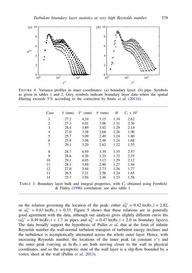
3.2. Variances
In figure 4, profiles of the streamwise variances u2+ are shown in inner coordinates,with the boundary layer data on the left and the pipe flow data on the right. Points inthe boundary layer data where the spatial filtering correction is greater than 5 % areindicated by grey symbols. The two flows show a broadly similar behaviour with adistinct inner peak at approximately the same wall-normal position. The inner peakappears to be invariant with Reynolds number, with a non-dimensional magnitudeu2+
I = 8.4± 0.8 for the boundary layer data, which agrees with the pipe data withinexperimental error. However, the inner peak values for the boundary layer are onlyresolved for the three lowest Reynolds numbers tested (2622 6 Reτ 6 8261). Thus,the data cannot resolve the question regarding the scaling of the inner peak at higherReynolds numbers.
The data indicate that an outer peak emerges at approximately the same Reynoldsnumber for the two flows. The outer peak magnitude, u2+
II , was found for eachReynolds number (for the three lowest Reynolds numbers there is no peak, and sothe inflection point was used instead), and the results shown in figure 5 demonstratethat the magnitudes of the outer peaks are very similar in boundary layer and pipeflows.
Pullin et al. (2013) presented an analysis that supports a logarithmic increase in theouter peak value u2+
II with Reynolds number, with two possible relations depending
Turbulent boundary layer statistics at very high Reynolds number 379
2
4
6
8
10
0
2
4
6
8
10
0100 104102 100 104102
(a) (b)
FIGURE 4. Variance profiles in inner coordinates: (a) boundary layer; (b) pipe. Symbolsas given in tables 1 and 2. Grey symbols indicate boundary layer data where the spatialfiltering exceeds 5 % according to the correction by Smits et al. (2011b).
TABLE 3. Boundary layer bulk and integral properties, with Cf obtained using Fernholz& Finley (1996) correlation; see also table 1.
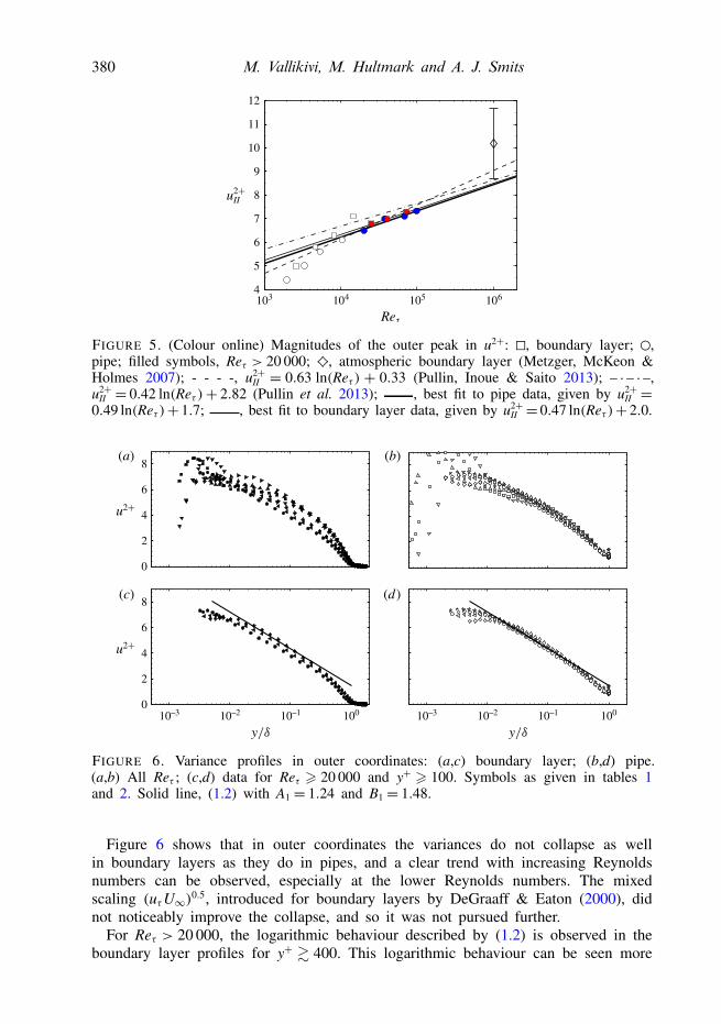
on the relation governing the location of the peak: either u2+II = 0.42 ln(Reτ ) + 2.82,
or u2+II = 0.63 ln(Reτ ) + 0.33. Figure 5 shows that these relations are in generally
good agreement with the data, although our analysis gives slightly different curve fits(u2+
II = 0.49 ln(Reτ ) + 1.7 in pipes and u2+II = 0.47 ln(Reτ ) + 2.0 in boundary layers).
The data broadly support the hypothesis of Pullin et al. that at the limit of infiniteReynolds number the wall-normal turbulent transport of turbulent energy declines andthe turbulence is asymptotically attenuated across the whole outer layer. Hence, withincreasing Reynolds number, the locations of the inner peak (at constant y+) andthe outer peak (varying as ln Reτ ) are both moving closer to the wall in physicalcoordinates, and so the asymptotic state of the wall layer is a slip-flow bounded by avortex sheet at the wall (Pullin et al. 2013).
II = 0.42 ln(Reτ )+ 2.82 (Pullin et al. 2013); , best fit to pipe data, given by u2+II =
0.49 ln(Reτ )+ 1.7; , best fit to boundary layer data, given by u2+II = 0.47 ln(Reτ )+ 2.0.
0
2
4
6
8
0
2
4
6
8
10–210–3 10–1 100 10–210–3 10–1 100
(a) (b)
(c) (d)
FIGURE 6. Variance profiles in outer coordinates: (a,c) boundary layer; (b,d) pipe.(a,b) All Reτ ; (c,d) data for Reτ > 20 000 and y+ > 100. Symbols as given in tables 1and 2. Solid line, (1.2) with A1 = 1.24 and B1 = 1.48.
Figure 6 shows that in outer coordinates the variances do not collapse as wellin boundary layers as they do in pipes, and a clear trend with increasing Reynoldsnumbers can be observed, especially at the lower Reynolds numbers. The mixedscaling (uτU∞)0.5, introduced for boundary layers by DeGraaff & Eaton (2000), didnot noticeably improve the collapse, and so it was not pursued further.
For Reτ > 20 000, the logarithmic behaviour described by (1.2) is observed in theboundary layer profiles for y+ & 400. This logarithmic behaviour can be seen more
Turbulent boundary layer statistics at very high Reynolds number 381
10
15
20
25
30
0
2
4
6
8
10
15
20
25
30
0
2
4
6
8
10
15
20
25
30
0
2
4
6
8
10
15
20
25
30
0
2
4
6
8
101520253035
0
2
4
6
8
101520253035
0
2
4
6
8
103101
101
102 104
102 103 104 105
101 102 103 104 105
103101 102 104
103101 102 104
10–2 100 10–2 100
10–2 100 10–2 100
10–2 10–110–3
10–1
10–1
10–3
10–3
100 10–2 10–110–3
10–110–3
10–110–3
100
101 102 103 104 105
(a) (b)
(c) (d)
(e) ( f )
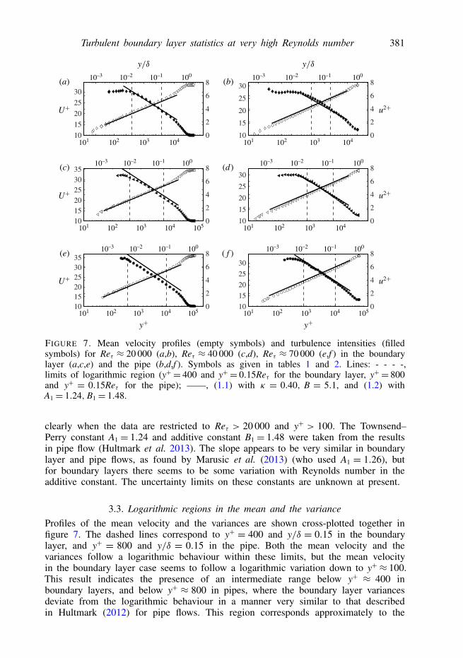
FIGURE 7. Mean velocity profiles (empty symbols) and turbulence intensities (filledsymbols) for Reτ ≈ 20 000 (a,b), Reτ ≈ 40 000 (c,d), Reτ ≈ 70 000 (e,f ) in the boundarylayer (a,c,e) and the pipe (b,d,f ). Symbols as given in tables 1 and 2. Lines: - - - -,limits of logarithmic region (y+= 400 and y+= 0.15Reτ for the boundary layer, y+= 800and y+ = 0.15Reτ for the pipe); ——, (1.1) with κ = 0.40, B = 5.1, and (1.2) withA1 = 1.24, B1 = 1.48.
clearly when the data are restricted to Reτ > 20 000 and y+ > 100. The Townsend–Perry constant A1 = 1.24 and additive constant B1 = 1.48 were taken from the resultsin pipe flow (Hultmark et al. 2013). The slope appears to be very similar in boundarylayer and pipe flows, as found by Marusic et al. (2013) (who used A1 = 1.26), butfor boundary layers there seems to be some variation with Reynolds number in theadditive constant. The uncertainty limits on these constants are unknown at present.
3.3. Logarithmic regions in the mean and the varianceProfiles of the mean velocity and the variances are shown cross-plotted together infigure 7. The dashed lines correspond to y+ = 400 and y/δ = 0.15 in the boundarylayer, and y+ = 800 and y/δ = 0.15 in the pipe. Both the mean velocity and thevariances follow a logarithmic behaviour within these limits, but the mean velocityin the boundary layer case seems to follow a logarithmic variation down to y+≈ 100.This result indicates the presence of an intermediate range below y+ ≈ 400 inboundary layers, and below y+ ≈ 800 in pipes, where the boundary layer variancesdeviate from the logarithmic behaviour in a manner very similar to that describedin Hultmark (2012) for pipe flows. This region corresponds approximately to the
382 M. Vallikivi, M. Hultmark and A. J. Smits
TABLE 4. Cases chosen for comparing boundary layer (current data) and pipe flow(Hultmark et al. 2013).
mesolayer described by Afzal (1982, 1984), George & Castillo (1997), Sreenivasan &Sahay (1997), Wosnik, Castillo & George (2000) and Wei et al. (2005) in boundarylayers, and the power law region described by McKeon et al. (2004) in pipes.George & Castillo (1997) suggested that in this region the mean velocity has reacheda seemingly logarithmic behaviour but the effects of viscosity are still evident in thebehaviour of the turbulent stress terms. Wei et al. (2005) identified the mesolayer withthe region where the stress gradients are close to zero, and the viscous force balancesthe pressure force in pipe flow or the mean advection in the turbulent boundary layer.The present results are at a sufficiently high Reynolds number to distinguish themesolayer clearly from the logarithmic region where all viscous effects are negligible,but a more precise statement needs a consideration of the spectral behaviour, whichis given by Vallikivi et al. (2015).
3.4. Higher-order momentsWe now consider the behaviour of the higher-order moments of the streamwisevelocity fluctuations (up to 10th order). Because no established correction for spatialfiltering on higher-order moments exists, data with more than 5 % spatial filtering onthe variances, as indicated by the spatial filtering correction, were excluded from theanalysis.
To make direct comparisons between boundary layer and pipe flows, six cases withmatching Reynolds numbers were chosen: cases 1–3 and 5–7 given in table 1 for theboundary layer, and cases 1–6 given in table 2 for the pipe. These cases correspondto Reτ ≈ 3000, 5000, 10 000, 20 000, 40 000, and 70 000, and they are summarizedin table 4. The higher-order moments for the pipe are reported here for the first time,although they are based on the data collected by Hultmark et al. (2013).
Figure 8 shows, for a representative boundary layer case, the probability densityfunction P(u) (p.d.f.), and the premultiplied probability density function u2pP(u),where 2p= [2, 6, 10] indicates the pth even moment. Each moment is the area underthe corresponding curve, and the data appear to be statistically converged. We see aclear deviation around the maximum value in the p.d.f. from a Gaussian behaviour,as well as deviations from symmetry in the premultiplied p.d.f.s.
The skewness S=〈u3〉/〈u2〉3/2 is shown in figure 9. Both flows exhibit a very similarbehaviour, with the skewness slightly positive near the wall for y+<200 and becomingnegative further away from the wall. For the boundary layer, the skewness is wellcollapsed in inner coordinates over the region 100 < y+ < 0.15Reτ , and we see allprofiles change sign at y+≈ 200 and reach a value of S≈−0.1 before becoming more
Turbulent boundary layer statistics at very high Reynolds number 383
0.5
0.6
0.1
0
0.2
0.3
0.4
0.02
0.01
0
0.03
0.04
0.05
–2 0 2 –2 0 2u u
(a) (b)
FIGURE 8. (Colour online) Probability density functions for the boundary layer at Reτ =70 000, y+ = 800. (a) u, P(u); ——, Gaussian distribution. (b) u2pP(u); p, 2p = 2; r,2p= 6;q, 2p= 10.
0.5
0
–0.5
–1.0
0.5
0
–0.5
–1.0
103101 102 104 105 103101 102 104 105
10–110–3 10–2 100 10–110–3 10–2 100
(a) (b)
(c) (d)
FIGURE 9. Skewness in inner coordinates (a,b) and outer coordinates (c,d) for cases givenin table 4. (a,c) Boundary layer; (b,d) pipe.
negative in the wake, where they collapse well in outer coordinates. In contrast, thepipe flow profiles show a small Reynolds number dependence over the log region, andthe collapse in the wake region in terms of outer layer coordinates is not as clean asthat seen in the boundary layer data.
The kurtosis K=〈u4〉/〈u2〉2 is shown in figure 10. Again, the behaviour for the twoflows is very similar, with perhaps some small dependence on the Reynolds numberin the outer region (although this could also be the result of some unresolved spatialfiltering effects).
384 M. Vallikivi, M. Hultmark and A. J. Smits
4.0
3.5
3.0
2.5
2.0
4.0
3.5
3.0
2.5
2.0
103101 102 104 105 103101 102 104 105
10–110–3 10–2 100 10–110–3 10–2 100
K
K
(a) (b)
(c) (d)
FIGURE 10. Kurtosis in inner coordinates (a,b) and outer coordinates (c,d) for cases givenin table 4. (a,c) Boundary layer; (b,d) pipe.
The pth roots of the pth even moments 〈(u+)2p〉1/p are shown in figure 11 for 2p=2,6, and 10 (the data for 2p= 4, 8, and 12 show the same trends). In inner coordinates,the behaviour is qualitatively similar to that seen in the variances, with an inner peakat about y+ = 15 that is either increasing very slowly with Reynolds number or notat all, a blending region over the range 30 < y+ < 300, followed by a logarithmicregion. The results from the boundary layer and the pipe agree well throughout mostof the flow, with the only differences appearing in the outer layer due to the differentouter boundary conditions, as expected. Some minor differences can also be seen inthe near-wall region, around y+ ≈ 15, where the pipe flow displays a slightly higherpeak value, possibly due to smaller spatial filtering effects since `+ is smaller for thepipe than the boundary layer (see table 4). Finally, it appears that the inner limit ofthe logarithmic range for pipes occurs at higher values of y+ than in boundary layers,similar to what was observed for the variances.
Figure 11 also displays the data in outer coordinates for the three highest Reynoldsnumbers (Reτ > 20 000). As seen in the variances, the higher moments show goodagreement between boundary layer and pipe flows. With increasing moment, theagreement improves, and the range of logarithmic behaviour increases.
The constants Ap and Bp in (1.3) were found by regression fit to each profile, that is,separately for each flow, Reynolds number, and moment. To test the consequences ofchoosing a particular range for the curve fit, different ranges were used for fitting, withthe inner limit varying as y+min = [3Re0.5
τ ; 200; 400; 600; 800] while keeping a constantouter limit at (y/δ)max= 0.15 (the results were not sensitive to reasonable variations inthe outer limit). A minimum of four points in each profile were used for determiningthe constants, otherwise the profile was discarded as not having a sufficiently extensivelogarithmic region.
The variation of the slope Ap with p is shown in figure 12. For Gaussian statistics,Ap would vary as A1[(2p − 1)!!]1/p, where A1 is the Townsend–Perry constant and !!denotes double factorial. It is evident that for boundary layer and pipe flows all theconstants have a sub-Gaussian behaviour, as observed by Meneveau & Marusic (2013)
Turbulent boundary layer statistics at very high Reynolds number 385
0
5
10
15
0
5
15
25
0
3
6
9
103101 102 104 105 10–110–3 10–2 100
(a) (b)
(c) (d)
(e) ( f )
FIGURE 11. Higher-order even moments 2p = 2, 6, and 10 for boundary layer (filledsymbols) and pipe flow (empty symbols). Data in inner coordinates (a,c,e) for all casesgiven in table 4. Same data in outer coordinates (b,d,f ) for Reτ > 20 000 and y+ > 100.Solid line, (1.3) with Ap and Bp derived from the pipe flow profile at Reτ = 70 000 (whereAp = [1.13; 2.48; 3.44] and Bp = [1.17; 3.31; 6.73] accordingly).
for boundary layers at lower Reynolds numbers. For smaller y+min values, there is aclear Reynolds number dependence in Ap between cases, as well as a dependence ony+min. For both flows, Ap was found to become independent of Reτ for y+min & 400. Thelimit y+min= 3Re0.5
τ used by Meneveau & Marusic (2013) underestimates the inner limitat low Reτ while overestimating it at high Reτ , and so it appears that either a constantinner limit or one with a very weak Reτ dependence is more appropriate for bothflows. A good representation of the asymptotic value of the slope is given empiricallyby Ap ∼ A1(2p− 1)1/2 for both pipe and boundary layer (A1 = 1.24, as before).
It appears that if a large enough value of y+min is chosen, Ap is independent ofReynolds number in pipe and boundary layer flows. The only outlier, the highestReynolds number case for the boundary layer, has a slightly lower value of Ap, butthis could be due to experimental error, which is expected to be greatest at the highestReynolds number.
The behaviour of the additive constant Bp is more difficult to establish, due to itshigh sensitivity to the magnitude of the moments. In pipes the constant appears tobe independent of Reynolds number, whereas in boundary layers a weak dependenceis observed in most cases. In contrast, Meneveau & Marusic (2013) found a muchstronger dependence, possibly caused by using 3Re0.5
τ as the inner limit on the curve
386 M. Vallikivi, M. Hultmark and A. J. Smits
2
4
6
2
4
6
2
4
6
2
4
6
2
2p 2p4 6 8 10 12
2
4
6
2 4 6 8 10 12
(a) (b)
(c) (d)
(e) ( f )
(g) (h)
(i) ( j)
FIGURE 12. Constant Ap for even moments 2p, for the fitting range y+ = [y+min, 0.15Reτ ].Left: boundary layer; right: pipe. Line colors given in table 4. ——, expected Gaussianvariation Ap = A1[(2p− 1)!!]1/p; - - - -, empirical fit Ap = A1(2p− 1)1/2.
fit. Interestingly, for the current data set Bp reached a constant value for the threehighest Reynolds number cases when y+min > 600 was used as inner limit, whichcould suggest that high-order moments are still affected by viscosity for smallery+. However, these trends are probably within experimental error, and no strongconclusions can be made.
4. Conclusions
Zero-pressure-gradient turbulent boundary layer measurements for 2600 < Reτ <72 500 were compared with previously acquired pipe flow data at similar Reynoldsnumbers. These Reynolds numbers covered a sufficient range to enable identificationof some apparently asymptotic trends. For Reτ > 20 000, the mean velocity andvariance profiles showed extended logarithmic regions, with very similar constants inboth flows. The two logarithmic regions coincide over the region 400. y+. 0.15Reτ .The inner limit may not be a perfect constant but may be subject to a weak Reynoldsnumber dependence (certainly less than Re0.5
τ ), and it is further explored by Vallikiviet al. (2015) when considering the spectral behaviour.
Turbulent boundary layer statistics at very high Reynolds number 387
Higher-order even moments also show a logarithmic behaviour over the samephysical space as the mean velocity and the variances, and the slope of the lineappears to become independent of Reynolds number for the same region, defined by400 . y+ . 0.15Reτ for both boundary layer and pipe flows. These bounds definea Reynolds number of Reτ ≈ 27 000 where this region extends over a decade iny+, underlining the need to obtain data at Reynolds numbers comparable to thoseobtained here if one wants to study scaling behaviours.
AcknowledgementsThe authors would like to thank B. McKeon and acknowledge J. Allen for their
help in the design and construction of the flat-plate apparatus and the pressuregradient blister, G. Kunkel, R. Echols and S. Bailey for conducting preliminarytests, and B. Ganapathisubramani and W. K. George for many insightful discussionsand suggestions. This work was made possible by support received through ONRgrant N00014-13-1-0174, program manager R. Joslin, and NSF grant CBET-1064257,program managers H. Winter and D. Papavassiliou.
REFERENCES
AFZAL, N. 1982 Fully developed turbulent flow in a pipe: an intermediate layer. Ing.-Arch. 52,355–377.
AFZAL, N. 1984 Mesolayer theory for turbulent flows. AIAA J. 22, 437–439.BAILEY, S. C. C., HULTMARK, M., MONTY, J. P., ALFREDSSON, P. H., CHONG, M. S., DUNCAN,
R. D., FRANSSON, J. H. M., HUTCHINS, N., MARUSIC, I., MCKEON, B. J., NAGIB, H. M.,ÖRLÜ, R., SEGALINI, A., SMITS, A. J. & VINUESA, R. 2013 Obtaining accurate meanvelocity measurements in high Reynolds number turbulent boundary layers using Pitot tubes.J. Fluid Mech. 715, 642–670.
BAILEY, S. C. C., KUNKEL, G. J., HULTMARK, M., VALLIKIVI, M., HILL, J. P., MEYER, K. A.,TSAY, C., ARNOLD, C. B. & SMITS, A. J. 2010 Turbulence measurements using a nanoscalethermal anemometry probe. J. Fluid Mech. 663, 160–179.
BAILEY, S. C. C., VALLIKIVI, M., HULTMARK, M. & SMITS, A. J. 2014 Estimating the value ofvon Kármán’s constant in turbulent pipe flow. J. Fluid Mech. 749, 79–98.
CLAUSER, F. H. 1956 The turbulent boundary layer. Adv. Mech. 4, 1–51.COLES, D. E. 1956 The law of the wake in the turbulent boundary layer. J. Fluid Mech. 1, 191–226.DEGRAAFF, D. B. & EATON, J. K. 2000 Reynolds-number scaling of the flat-plate turbulent boundary
layer. J. Fluid Mech. 422, 319–346.FERNHOLZ, H. H. & FINLEY, P. J. 1996 The incompressible zero-pressure-gradient turbulent boundary
layer: an assessment of the data. Prog. Aerosp. Sci. 32, 245–311.GEORGE, W. K. & CASTILLO, L. 1997 Zero-pressure-gradient turbulent boundary layer. Appl. Mech.
Rev. 50, 689–729.HULTMARK, M. 2012 A theory for the streamwise turbulent fluctuations in high Reynolds number
pipe flow. J. Fluid Mech. 707, 575–584.HULTMARK, M. & SMITS, A. J. 2010 Temperature corrections for constant temperature and constant
current hot-wire anemometers. Meas. Sci. Technol. 21, 105404.HULTMARK, M., VALLIKIVI, M., BAILEY, S. C. C. & SMITS, A. J. 2012 Turbulent pipe flow at
extreme Reynolds numbers. Phys. Rev. Lett. 108 (9), 1–5.HULTMARK, M., VALLIKIVI, M., BAILEY, S. C. C. & SMITS, A. J. 2013 Logarithmic scaling of
turbulence in smooth- and rough-wall pipe flow. J. Fluid Mech. 728, 376–395.HUTCHINS, N., CHAUHAN, K. A., MARUSIC, I., MONTY, J. & KLEWICKI, J. 2012 Towards
reconciling the large-scale structure of turbulent boundary layers in the atmosphere andlaboratory. Boundary-Layer Meteorol. 145, 273–306.
388 M. Vallikivi, M. Hultmark and A. J. Smits
JIMÉNEZ, J. M., HULTMARK, M. & SMITS, A. J. 2010 The intermediate wake of a body of revolutionat high Reynolds numbers. J. Fluid Mech. 659, 516–539.
MACMILLAN, F. A. 1957 Experiments on Pitot tubes in shear flow. No. 3028 Ministry of Supply,Aeronautical Research Council.
MARUSIC, I., MCKEON, B. J., MONKEWITZ, P. A., NAGIB, H. M., SMITS, A. J. & SREENIVASAN,K. R. 2010 Wall-bounded turbulent flows: recent advances and key issues. Phys. Fluids 22,065103.
MARUSIC, I., MONTY, J. P., HULTMARK, M. & SMITS, A. J. 2013 On the logarithmic region inwall turbulence. J. Fluid Mech. 716, R3,1–3.
MATHIS, R., HUTCHINS, N. & MARUSIC, I. 2009 Large-scale amplitude modulation of the small-scalestructures in turbulent boundary layers. J. Fluid Mech. 628, 311–337.
MCKEON, B. J., LI, J., JIANG, W., MORRISON, J. F. & SMITS, A. J. 2003 Pitot probe correctionsin fully developed turbulent pipe flow. Meas. Sci. Technol. 14 (8), 1449–1458.
MCKEON, B. J., LI, J., JIANG, W., MORRISON, J. F. & SMITS, A. J. 2004 Further observationson the mean velocity distribution in fully developed pipe flow. J. Fluid Mech. 501, 135–147.
MCKEON, B. J. & SMITS, A. J. 2002 Static pressure correction in high Reynolds number fullydeveloped turbulent pipe flow. Meas. Sci. Technol. 13, 1608–1614.
MENEVEAU, C. & MARUSIC, I. 2013 Generalized logarithmic law for high-order moments in turbulentboundary layers. J. Fluid Mech. 719, R1.
METZGER, M., MCKEON, B. J. & HOLMES, H. 2007 The near-neutral atmospheric surface layer:turbulence and non-stationarity. Phil. Trans. R. Soc. Lond. A 365 (1852), 859–876.
MILLIKAN, C. B. 1938 A critical discussion of turbulent flows in channels and circular tubes.In Proceedings of the fifth International Congress for Applied Mechanics, pp. 386–392.Wiley/Chapman and Hall.
NAGIB, H. M., CHAUHAN, K. A. & MONKEWITZ, P. A. 2007 Approach to an asymptotic state forzero pressure gradient turbulent boundary layers. Phil. Trans. R. Soc. Lond. A 365 (1852),755–770.
ÖSTERLUND, J. M., JOHANSSON, A. V., NAGIB, H. M. & HITES, M. H. 2000 A note on theoverlap region in turbulent boundary layers. Phys. Fluids 12 (1), 1–4.
PATEL, V. C. 1965 Calibration of the Preston tube and limitations on its use in pressure gradients.J. Fluid Mech. 23, 185–208.
PERRY, A. E., HENBEST, S. M. & CHONG, M. S. 1986 A theoretical and experimental study ofwall turbulence. J. Fluid Mech. 165, 163–199.
PULLIN, D. I., INOUE, M. & SAITO, N. 2013 On the asymptotic state of high Reynolds number,smooth-wall turbulent flows. Phys. Fluids 25 (1), 105116.
ROSENBERG, B. J., HULTMARK, M., VALLIKIVI, M., BAILEY, S. C. C. & SMITS, A. J. 2013Turbulence spectra in smooth- and rough-wall pipe flow at extreme Reynolds numbers.J. Fluid Mech. 731, 46–63.
SMITS, A. J. & MARUSIC, I. 2013 Wall-bounded turbulence. Phys. Today 25–30.SMITS, A. J., MCKEON, B. J. & MARUSIC, I. 2011a High Reynolds number wall turbulence. Annu.
Rev. Fluid Mech. 43, 353–375.SMITS, A. J., MONTY, J., HULTMARK, M., BAILEY, S. C. C., HUTCHINS, M. & MARUSIC, I.
2011b Spatial resolution correction for turbulence measurements. J. Fluid Mech. 676, 41–53.SREENIVASAN, K. R. & SAHAY, A. 1997 The persistence of viscous effects in the overlap region
and the mean velocity in turbulent pipe and channel flows. In Self-Sustaining Mechanisms ofWall Turbulence (ed. R. Panton), pp. 253–272. Comp. Mech. Publ.
TOWNSEND, A. A. 1976 The Structure of Turbulent Shear Flow. Cambridge University Press.VALLIKIVI, M. 2014 Wall-bounded turbulence at high Reynolds numbers. PhD thesis, Princeton
University.VALLIKIVI, M., GANAPATHISUBRAMANI, B. & SMITS, A. J. 2015 Spectra in boundary layers and
pipes at very high Reynolds numbers. J. Fluid Mech. 771, 303–326.VALLIKIVI, M., HULTMARK, M., BAILEY, S. C. C. & SMITS, A. J. 2011 Turbulence measurements
in pipe flow using a nano-scale thermal anemometry probe. Exp. Fluids 51, 1521–1527.
Turbulent boundary layer statistics at very high Reynolds number 389
VALLIKIVI, M., HULTMARK, M. & SMITS, A. J. 2013 The scaling of very high Reynolds numberturbulent boundary layers. In 8th International Symposium on Turbulence and Shear FlowPhenomena, Poitiers, France.
VALLIKIVI, M. & SMITS, A. J. 2014 Fabrication and characterization of a novel nano-scale thermalanemometry probe. J. Microelectromech. Syst. 23 (4), 899–907.
WEI, T., FIFE, P., KLEWICKI, J. C. & MCMURTRY, P. 2005 Properties of the mean momentumbalance in turbulent boundary layer, pipe and channel flows. J. Fluid Mech. 522, 303–327.
WINKEL, E. S., CUTBIRTH, J. M., CECCIO, S. L., PERLIN, M. & DOWLING, D. R. 2012 Turbulenceprofiles from a smooth flat-plate turbulent boundary layer at high Reynolds number. Exp. Therm.Fluid Sci. 40, 140–149.
WINTER, K. G. & GAUDET, L. 1970 Turbulent boundary-layer studies at high Reynolds numbersat Mach numbers between 0.2 and 2.8. R & M No. 3712. Aeronautical Research Council,Ministry of Aviation Supply, Royal Aircraft Establishment, RAE.
WOSNIK, M., CASTILLO, L. & GEORGE, W. K. 2000 A theory for turbulent pipe and channel flows.J. Fluid Mech. 421, 115–145.
ZAGAROLA, M. V. & SMITS, A. J. 1998 Mean-flow scaling of turbulent pipe flow. J. Fluid Mech.373, 33–79.
ZAGAROLA, M. V., WILLIAMS, D. R. & SMITS, A. J. 2001 Calibration of the Preston probe forhigh Reynolds number flows. Meas. Sci. Technol. 12, 495–501.