J. Fluid Mech. (2014), . 748, pp. doi:10.1017/jfm.2014.189 ... Flow JFM... · Radiofrequency plasma...

J. Fluid Mech. (2014), vol. 748, pp. 663–691. c© Cambridge University Press 2014doi:10.1017/jfm.2014.189

663

Radiofrequency plasma stabilization of alow-Reynolds-number channel flow

Timothy J. Fuller1, Andrea G. Hsu2, Rodrigo Sanchez-Gonzalez2,Jacob C. Dean2, Simon W. North2 and Rodney D. W. Bowersox1,†

1Aerospace Engineering, Texas A&M University, College Station, TX 77843, USA2Chemistry, Texas A&M University, College Station, TX 77843, USA

(Received 6 October 2013; revised 24 March 2014; accepted 2 April 2014;first published online 8 May 2014)

The effects of plasma heating and thermal non-equilibrium on the statisticalproperties of a low-Reynolds-number (Reτ = 49) turbulent channel flow were experi-mentally quantified using particle image velocimetry, two-line planar laser-inducedfluorescence, coherent anti-Stokes Raman spectroscopy and emission spectroscopy.Tests were conducted at two radiofrequency plasma settings. The nitrogen, in air,was vibrationally excited to Tvib ∼ 1240 K and 1550 K for 150 W and 300 Wplasma settings, respectively, while the vibrational temperature of the oxygen and therotational/translational temperatures of all species remained near room temperature.The peak axial turbulence intensities in the shear layers were reduced by 15 and 30 %in moving across the plasma for the 150 and 300 W cases, respectively. The plasmadid not alter the transverse intensities. The Reynolds shear stresses were reduced by30 and 50 % for the 150 and 300 W cases. The corresponding Reynolds shear stresscorrelation coefficient was also reduced, which indicates that the large-scale structureswere diminished. Finally, the plasma enhanced the turbulence decay in the zero-shearregions, where the power law decay t−1/n exponential factor n decreased from 1.0to 0.8.

Key words: low-Reynolds-number flows, plasmas, turbulent flows

1. Introduction1.1. Motivation and objectives

Relaminarization is a process where an initially turbulent flow returns to an effectivelylaminar state. Understanding and control of this process have important implicationsacross a myriad of disciplines ranging from reduced pressure drop in pipelines toreduced heat transfer in hypersonic flight systems. Also, as discussed by Sreenivasan(1982), relaminarizing flows have important uses in turbulence model validation.

In the 1980s to early 2000s, there was considerable research into the potentialuse of weakly ionized plasmas to control shock wave strength and structure inhigh-speed flow(Klimov et al. 1982; Ionikh et al. 1999; Merriman et al. 2001; Palmet al. 2003). It was ultimately determined that the observations were consistentwith conventional gas dynamic heating effects (Aleksandrov et al. 1986; Evtyukhin,

† Email address for correspondence: [email protected]

mailto:[email protected]

664 T. J. Fuller and others

Margolin & Shmelev 1986; Voinovich et al. 1991; Ionikh et al. 1999; Macheretet al. 2001; Palm et al. 2003). Pertinent to the present study, Palm et al. (2003)demonstrated that radiofrequency (RF) plasma heating of the viscous boundary layerswas an important process, where the observed shock weakening was absent when theboundary interaction was removed. The RF plasma heating effect on the boundarylayer is of interest as there are many related mechanisms reported to stabilizeboundary layer turbulence (Narasimha & Sreenivasan 1979). These mechanisms arehighlighted in § 1.2. In addition to these processes, RF plasma introduces thermalnon-equilibrium (electronic and vibrational), which may affect the stability of the flow.

The objective of this study is to experimentally quantify the effects of plasmaheating and thermal non-equilibrium on the statistical properties of a relaminarizingchannel flow. The study was performed in an ∼4:1 aspect ratio duct, with animposed RF plasma. Downstream of the plasma, the nitrogen, in air, was vibrationallyexcited. The mean and turbulent flow properties were quantified using particle imagevelocimetry (PIV), planar laser-induced fluorescence, dual-pump broadband coherentanti-Stokes Raman spectroscopy (CARS) and emission spectroscopy. Following thesuggestion of Sreenivasan (1982), data were collected to allow for full documentationof the inflow conditions, as well as to enable integral momentum and energy balances.In this paper, we describe the experimental methods, present the measurements, anddiscuss the effects of the plasma on the mean and turbulent flow evolution.

1.2. Relaminarization mechanismsIncrease of the dissipation, which is equivalent to lowering of the Reynolds number,is a stabilizing mechanism (Narasimha & Sreenivasan 1979) that has been shown tolead to reverse transition in a two-dimensional channel flow (Narayanan 1968). Thecritical Reynolds number for relaminarization was estimated at ∼1400 based on theduct half-height and mean axial velocity. Also, in that study, the Reynolds normalstresses decreased exponentially, whereas the Reynolds shear stresses tended to zeroat a well-defined location. This observation implied a loss of coherent structure(Narasimha & Sreenivasan 1979). This mechanism is important to the present study,as the plasma increases the temperature and hence lowers the Reynolds number.

Density stratification is a stabilization process, where turbulent energy is expendedto overcome a stabilizing density gradient (Narasimha & Sreenivasan 1979). Thismechanism is most often associated with buoyancy-driven flows. However, Nicholl(1970) measured reduced velocity fluctuations in a wind tunnel wall boundary layerpassing over a step increase in the wall temperature. Thus, density stratification isrelevant as the present RF plasma source resulted in wall heating near the electrodes.

Acceleration and streamline curvature are both stabilizing processes (Bradshaw1969, 1973). The primary explanations are reduced production (Arnette, Samimy& Elliott 1998), pressure forces (Narasimha & Sreenivasan 1979),bulk dilatation(Dussauge & Gaviglio 1987) and large-scale structure reduction (Luker, Bowersox& Buter 2000). Many parameters have been proposed to characterize these effects(Spina, Smits & Robinson 1994). Bradshaw (1973) points out that the response ofthe flow is about an order of magnitude larger than would be expected based on theextra production. Launder, Reece & Rodi (1975) explained this discrepancy via theirpressure–strain redistribution model and Tichenor, Humble & Bowersox (2013) foundthat this model reproduced the stabilization observed in a Mach 5 flow with a convexcurvature-driven pressure gradient. Interestingly, the low-speed study of Narayanan(1968) did not show evidence of a loss in correlation in the Reynolds stress. However,

Plasma stabilization of a low-Reynolds-number channel flow 665

significant reductions, and even sign changes, are present in many supersonic studies(Arnette et al. 1998; Luker et al. 2000 and Tichenor et al. 2013). These processesare relevant to the present study as the thermal heating near the electrodes resultedin boundary layer displacement, and hence acceleration and streamline curvature.

Ekoto et al. (2009) established that boundary layer turbulence responds to pressurewaves emanating from small-scale surface roughness, and the response follows thelarger-scale curvature trends. This small-scale effect is important to this study as theRF plasma was confined to a relatively short axialdistance (∼1/2 the channel height).

The coherent horseshoe, or hairpin, structure of turbulence, which is responsiblefor near-wall production, has been studied extensively since the 1950s (Theodorsen1952; Kline et al. 1967; Kim, Kline & Reynolds 1971; Robinson 1991; Panton 1997).Christensen & Adrian (2001) defined a hairpin vortex to include quasi-streamwisevortices that may have the shape of a hairpin or cane, where the arch vortex isstrong enough to induce an ejection event beneath it. Schoppa & Hussain (2002)presented a transient growth mechanism capable of producing linear amplificationof x-dependent disturbances. They also showed a drag reduction control strategybased on this mechanism. All of the mechanisms in the previous paragraphs have thepotential to influence the production of turbulence by altering this underlying streakstructure of the turbulence.

Recent high-speed transition studies provide evidence that vibrational non-equilibrium can introduce stabilizing effects into fluid mechanical processes (Fujii& Hornung 2003; Leyva et al. 2009). The numerical work of Osipov, Uvarov &Vinnichenko (2006) also provides evidence that vibrational non-equilibrium canaffect the structure of the vorticity within a Kármán vortex sheet. These thermalnon-equilibrium processes are relevant to the present study, as the air moleculesexperienced significant electronic excitation within the RF plasma, and the nitrogenexited the plasma in a vibrationally excited state. The rotational and translationalenergy levels remained close to their ground state room temperature values, as did theoxygen vibrational temperature. Vibrational decay, and the corresponding translationaltemperature rise, occurred on a time scale similar to that of the turbulence decaywithin the duct.

Martin & Candler (1998) demonstrated through direct numerical simulation apositive feedback between thermal fluctuations and chemical heat release, whereheat release resulted in larger temperature fluctuations, which in turn increased thechemical heat release. Simultaneously, they observed localized shocks and expansionsthat fed energy into the turbulent kinetic energy via the pressure–strain term. Thisexample of thermal–mechanical coupling is relevant here as the reported mechanismsare similar to those expected with the plasma.

Magnetized magnetohydrodynamic (MHD) turbulence is another example of acoupled energy exchange mechanism for velocity–velocity, velocity–magnetic andmagnetic–magnetic modes (Vedenov 1968; Biskamp 1993, 2000, 2003; Falgarone &Passot 2003; Verma 2004). Coupling due to polarized waves (Chen, Chen & Eyink2003; Galtier & Bhattacharjee 2003; Cho 2011; Zhu, Yang & Zhu 2014) and MHDbody forces (Maden et al. 2013) can affect the hydrodynamics. However, externalmagnetic fields were not employed in the present study.

2. Experimental methods2.1. Facility flow path

A circuit-type wind tunnel was constructed and equipped with an RF plasmageneration system to introduce vibrational non-equilibrium into basic decaying mesh


(b)

(a)

(c) (d)

Flow conditioning& contraction

Turbulence generator Test section

Diffuser

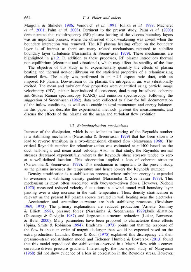
FIGURE 1. Photographs of the facility and plasma. (a) Facility. (b) Ceramic plasmasection. (c) Plasma electrode. (d) Plasma.

and channel flows. The circuit was constructed from 20.3 cm diameter polyvinylchloride (PVC) piping. An axial fan (Hartzell 4616DH3) powered by a pneumaticmotor (Atlas Copco Tools LZB 33L A060-11) drove the flow. A vacuum system(Leybold E250 backing pump/RUVAC WAU 1001 Roots blower) was used to maintaina system stagnation pressure of 30 Torr ± 2.0 %. The stagnation temperature was295 K± 1.0 %.

A photograph of the test section is given in figure 1(a). Before the flow entered thetest section, it was conditioned through honeycomb straighteners, a stilling chamber(located at x/M =−52.5) and a contraction. The ratio of the contraction was 16.3:1with sidewall half-angles of 4.8◦. The test section was located downstream of theadjustable turbulence generation chamber and included the plasma generation assemblywith embedded electrodes (described in § 2.2). The turbulence was generated with apassive grid (described later), and M is the grid mesh spacing. The majority of thetest section components were fabricated from aluminium to ensure structural rigidity;see figure 1(b). The test section width was fixed at 10.16 cm. The adjustable upperand lower walls were fixed at half-angles of 0.18◦ to promote a constant average flowvelocity. The divergence began immediately downstream of the passive grid (origin ofthe axial coordinate, x) with an initial height of 1.91 cm. The duct height, 2δ, is givenby 1.91+ 0.0063x (cm); the coordinate system is described in the next paragraph. Aschematic of the contraction and test section flow path is plotted in figure 2. Ceramic(Macor) inserts were used to form the structure around the plasma discharge to bothelectrically isolate the electrodes and mitigate heat damage from intermittent plasmaarcing. Both sidewalls were equipped with fused silica windows to provide opticalaccess upstream and downstream of the plasma discharge.

The coordinate system is shown in figure 2. The origin of the axial coordinate, x,was located at the downstream face of the turbulence grid. The origin of the transversecoordinate, y, was located along the centreline of the facility.

The tunnel stagnation pressure was measured just upstream of the contraction(x/M =−40) with a 0.79 mm diameter Pitot tube instrumented with an MKS Series


0–5–10–10

–5

0y/M

5

10

–15–20–25–30–35–40 5

x/M10 15 20 25 30 35 40 45 50

FIGURE 2. Internal flow path (flow is left to right).

x/M a RF power (kW) um (m s−1) Pb (Torr) T (K) Re2δ Reτ

14.0 0 20.7 29.9 295 1100 4926.9 0 20.5 29.9 292 1100 4426.9 150 22.4 29.9 319 1100 4526.9 300 23.6 29.9 336 1100 45a uref = 20.7, Tref = 295 K.b Computed using the integral methods in § 4.

TABLE 1. Operating conditions.

902 pressure transducer (1000 Torr, ±1.0 % of the reading). The facility temperature(T) was monitored with an Omega brand type-K thermocouple, which was accurateto within ±2 K. The operating conditions are listed in table 1. Also listed in table 1are the duct height and viscous Reynolds numbers given by Re2δ = um2δ/ν andReτ = uτδ/ν (=δ+), respectively. In these relations um is the mean velocity, uτ is thefriction velocity and ν is the kinematic viscosity.

A passive grid was located in the turbulence generation chamber 8.89 cm down-stream of the contraction. The grid used in the present study is shown schematicallyin figure 3. The grid mesh size (M), the bar size (DM) and the porosity (βM)were 15.24 mm, 5.08 mm and 52 %, respectively. The perimeter grid surfaces weremachined to form seamless transitions with the adjoining inner wall surfaces of thefacility in order to avoid steps in the internal flow path. The mesh Reynolds number,given by ReM = umM/ν, was 800. The grid elements were generated by millingvertical slots 3.18 mm deep into the upwind face and horizontal slots 3.18 mm deepinto the downwind face. All bar edges were left as sharp as possible to aid in theturbulence generation. The small radii left in the corners of each slot from machiningwere filed square. The downstream face of the grid was located at x/M = 0.

2.2. Plasma generationA 2500 W, 200 V, 13.56 MHz RF generator source (Dressler Cesar Model 1325)was used to generate a sustained plasma discharge within the test section. Vibrationaltemperatures of the order of Tvib∼ 1200–2000 K were produced, while the translationand rotational temperatures remained close to room temperature. The generator wasconnected to a 2–27 MHz, 700–1500 W Variomatch matching network. Due tothe limited impedance range within the matching network, the output power waspassed through an external copper inductor coil (6.35 mm diameter) to add additionalimpedance. The RF plasma was discharged between two copper electrodes embedded


7.26 10.16

15.24

5.08

5.08

FIGURE 3. Grid, where the flow is out of the page (dimensions: mm).

into dielectric ceramic plates forming the top and bottom walls of the test-section; seefigure 1(b). Each electrode assembly included tilt adjustment. The electrodes used inthis study had circular cross-sections and were made of copper. The electrodes were7.6 cm long cylinders (1.52 cm diameter) with hemispherical ends (3.7 cm radius);see figure 1(c) for a photograph of an electrode. The plasma discharge ignition andstability were highly dependent on both the stagnation pressure and the electrodegap. The optimal configuration for plasma stability consisted of an electrode gapof 3.0 cm and a pressure of 30 Torr. A photograph of a typical plasma is shownin figure 1(d). The plasma settings utilized in this study are listed in table 1. Theelectron temperature was not measured; however, based on previous studies withsimilar configurations and operating conditions, it is expected to be in the rangeof 1–3 eV (Raizer 1997; Palm et al. 2003; Montello et al. 2012). The neutral andion temperatures remained near room temperature (0.025–0.029 eV) as the flowexperienced modest heating (see table 1). Similarly, the electron and ion numberdensities were <1× 1011 cm−3.

The location of the electrodes was centred on xp/M = 15.9. Moderate heatingof the ceramic plates housing the electrodes was observed during operation. Theplasma visually appeared to be centred in the spanwise direction and was nominallytrapazoidally shaped. The width decreased from ∼7.5 cm near the floor to ∼5.0 cmnear the ceiling of the test section. The axial length of the plasma region wasestimated at ∼1 cm. Bright bands near the surfaces extended donwstream as near-wallplasma streaks. These streaks are visible on the right edge, as bright regions, infigure 4(a) (in § 2.3). The rightmost peak of these tails was located nominally 20 %of the duct half-height (δ) from each wall, which corresponds to y+ ∼ 12, wherey+ = uτy/ν.

2.3. Particle image velocimetry (PIV)The PIV system consisted of a New Wave Solo 120 XT dual-head double-pulsedfrequency-doubled Nd:YAG laser, which produced two 3–5 ns, 120 mJ/pulse laserbeams at a wavelength of 532 nm. The available laser repetition rate was 15 Hz andthe interpulse separation for each laser was set to 9.0 µs. The thickness of the lasersheet within the test section was less than 0.5 mm.

The tunnel was seeded with a TSI six-jet atomizer operating with di(2-ethylhexyl)sebacate (DEHS), which produced polydisperse particles with a mean diameter ofapproximately 300 nm. For the present flow conditions, the Knudsen number basedon the mean particle diameter was 13. Hence, the time response of the particles wasestimated as τr (ms)= d2

pρpCC/18µ, where CC is a correction factor for low-density


(a) (b)

FIGURE 4. Example PIV image at x/M= 17.7 (flow is from left to right). (a) Raw image.(b) Image with background subtraction.

x, y (mm) P T ua (u′i2)1/2/u u′v′/u2 Trot Tvib τwall

2.0, 0.3 2.0 % 1.0 % 0.5 % 2.5 % 15 % 5.0 % 5.0 % 10 %a The run-to-run axial velocity repeatability was of the order of 2 %.

TABLE 2. Uncertainty estimates.

effects. Following Loth (2008), CC=1+Kn(2.514+0.8e−0.55/Kn). For the present study,τr = 5 µs. Taking the characteristic flow time as τf = δ/um results in a Stokes number(τr/τf ) of 0.02, which indicates that the particles faithfully followed the flow (Menon& Lai 1991). The particle concentration was estimated as of the order of 1×105 cm−3

via visual inspection of the PIV images.The sample set at each location consisted of 3450 image pairs. The first step

in reconstructing velocity fields was to perform average image subtractions, whichincreased the number of vectors by lowering the effects of weak reflections anda substantial portion of the strong reflections near the tunnel walls. The imagesubtraction also helped to remove the effects of the plasma glow. For example, theplasma streaks at the first location downstream of the plasma (figure 4a) are essentiallyremoved after the image subtraction (figure 4b). The velocity field reconstructionwas then accomplished using the dPIV 32-bit analysis code (v2.1) of InnovativeScientific Solutions, Inc. (ISSI). A three-step adaptive correlation procedure, usingsuccessive interrogation window sizes of 128 pixel × 128 pixel, 64 pixel × 64 pixeland 32 pixel × 32 pixel with 50 % overlap, was used. The 32 pixel × 32 pixel areacorresponded to a nominal 0.55 mm × 0.55 mm physical dimension. Correlationmultiplication and a consistency filter were used with the minimum number ofvectors and absolute distance both set to 2. The PIV 95 % confidence uncertaintieswere estimated following Benedict & Gould (1996) assuming a normal distribution forthe present large sample set. The estimates were based on a peak fluctuation of 10 %,which was the peak value in the boundary layer region for the first measurementstation. The results are summarized in table 2.

An important consideration in the present PIV experiments is the effect of theplasma on the particles. Specifically, as the particles traverse the plasma, they suffersignificant negative charging (Boeuf & Punset 1999; Shukla & Mamun 2002). Anorder of magnitude study of the particle charging and corresponding forces wasperformed to quantify the charging effects. The calculations were carried out for the


λDb 1p

b V∗ −Zp CDn CDi CE/E c Cth

4.0 200 −2.24 700 4× 101 10−8 10−4 10−2

a Te = 3 eV, Ti = 0.029 eV, nn = 8.7× 1017, ne = ni ≈ 1× 1011 cm−3.b µm.c (V−1 m).

TABLE 3. Plasma particle interaction estimates.a

conditions listed in the last row of table 1. For this analysis, the electron temperature(Te) was set to 3.0 eV, which is the upper limit of the expected range. Because theelectron temperature was significantly greater than the ion temperature (Ti=0.029 eV),the Debye shielding radius λD was essentially equivalent to that for ions. The ionvalue is given by λDi= (ε0kTi/e2ni)

1/2. In this expression, ε0 is the vacuum permittivity,k is the Boltzmann constant, Ti is the ion temperature, e is the electric charge carriedby a proton and ni is the number density of the ions (1 × 1011 cm−3). Hence,λD ≈ 4.0 µm. Because λD � rp (0.15 µm), the sheath is considered thick, and theparticle charging was estimated using the orbit-motion-limited (OML) theory for aspherical probe (Mott-Smith & Langmuir 1926; Allen 1992; Matsoukas & Russell1995). Moreover, the particle spacing ∆p (=n−1/3

d ) was visually estimated at ∼200 µm.Since ∆p � λD, the particle interaction is expected to be minimal, and hence eachparticle is treated as if in isolation.

The first step in the analysis is to estimate the equilibrium charge on the PIVparticles. Following Matsoukas & Russell (1995), the charge potential between theparticle and the plasma is found by setting the rate of change of the particle chargingto zero. Setting the sum of the electron and ion fluxes to the particle to zero resultsin

eV∗ =(

meTi

miTe

)1/2

− V∗(

meTe

miTi

)1/2

. (2.1)

In this expression, V denotes the reduced potential between the plasma andparticle given by eV(rp)/kTe, the asterisk denotes equilibrium and me and miare the electron and ion (N+2 ) masses, respectively. This equation was solvednumerically for V∗; the resulting value is included in table 3.Matsoukas & Russell(1995) also provide an approximation to the above relation, which is given byV∗ ' C ln(meTe/miTi)

1/2. With the constant C set to 0.73, the errors with thisapproximation compared with the numerical results from the above equation were<1 % for Te from 0.1 to 3.0 eV. The particle charge number, which is relatedto the charge potential by Zp = 4πε0kTerpV∗/e2 (Boeuf & Punset 1999), is alsolisted in table 3. The particle charging time is derived by integrating the particlecharge evolution equation. The resulting expression for the characteristic time scaleis τp = ε0(2πmikTe)

1/2/(1 − V∗)rpe2 (Boeuf & Punset 1999), which is ∼0.3 µs. Theparticle transit time through the nominally 1 cm long plasma was ∼400 µs. Thus,the particles achieved equilibrium charges in the plasma.

The second step in the analysis is to estimate the forces on the particles as theytraverse the plasma. The forces considered here include neutral drag, ion drag, theelectrostatic force and the thermophoretic force.

The Reynolds number based on the particle diameter is very low (Rep= 0.014), and,as mentioned earlier, the Knudsen number is nominally 13. Hence, the neutral drag


coefficient is given by a Stokes law corrected for low-density (Loth 2008), that is,

CDn ' 24/RepCC. (2.2)

The numerical value for the present study is listed in table 3.The ion drag has two parts, one due to the momentum exchange during a collision,

where the ion is collected, and the other due to the Coulomb momentum exchangeduring a deflection encounter. The total ion drag coefficient is given by Barnes et al.(1992),

CDi = nimi(σcoll + σ coul)vsui/

12ρu2

mπr2p, (2.3)

where the total speed is given by vs = (u2i + 8kTi/πmi)

1/2 and ui is the ion driftvelocity, taken as the bulk velocity through the plasma (um). The momentum exchangecross-sections are given by σ coll = πb2

c and σ coul = 4πb2π/2Γ , where bc = rp(1 −

−2V∗kTe/miv2s )

1/2, bπ/2' rp(−V∗kTe/miv2s ) and Γ = ln[(λ2

D+ b2π/2)/(b

2c + b2

π/2)]/2. Anorder of magnitude estimate is listed in table 3. As indicated, this effect is expectedto be insignificant.

The electric force coefficient is given by Shukla & Mamun (2002),

CE =Qp E/ 12ρu2

mπr2p. (2.4)

In this relation, Qp is the particle charge given by Qp = Zpe and E is the appliedelectric field. The order of magnitude estimate is listed in table 3. This effect isexpected to be insignificant as a very large field (∼1000 V cm−1) would be requiredto compete with the neutral drag. Even though the electric field for the RF plasmais expected to be ∼250 V cm−1, the relatively massive particles cannot respond tothe 13.56 MHz frequency. Hence, the particles respond to low-frequency induced orapplied fields, which were not present.

Lastly, the thermopheretic force is (Boeuf & Punset 1999)

Cth '−(2.1r2p/vth) kT1T/ 1

2ρu2mπr2

p, (2.5)

where vth is the thermal velocity of the neutral molecules (= vth = (8kT/πmn)1/2), kT

is the translational thermal conductivity of the neutral gas and T is the translationaltemperature of the neutral gas. The data in table 1, with a plasma length of ∼1 cm,indicated that the temperature gradient is ∼40 K cm−1. This order of magnitudeanalysis suggested that the thermophoretic force was insignificant compared to thedrag.

In summary, the present analysis indicates that charging and thermal forces hadminimal impact on the particle trajectories. Hence, it is expected that the PIV particlesadequately followed the flow.

2.4. Coherent anti-Stokes Raman spectroscopyCoherent anti-Stokes Raman spectroscopy (CARS) was used to assess the vibrationalenergy content of the dominant species, N2 and O2, along the test section centreline.Point measurements were performed at the plasma discharge location and atother multiple locations downstream. The determination of N2 and O2 vibrationaltemperatures was enabled by a dual-pump CARS system, requiring two differentnarrowband pump laser frequencies, ω1 and ω2, and one broadband Stokes laser beam,ωs (Lucht 1987). The CARS system consisted of an injection-seeded Spectra-Physics


Nd:YAG laser (PRO 290-10) operated at 10 Hz, which provided 800 mJ/pulse witha linewidth of 0.003 cm−1, when frequency doubled to 532 nm. The first pumpfrequency, ω1, accounted for 10 % of the 532 nm energy reflected from a quartzplate. The second pump frequency, ω2, was obtained by splitting approximately400 mJ/pulse from the remaining 532 nm beam used to pump a PDL2 dye laserthat produced a narrowband output at 555 nm using fluorescein in methanol. Theremaining 532 nm beam was used to pump a custom-built broadband dye laseroperated as the Stokes beam, ωs, producing ∼20 mJ/pulse centred at 607 nm usinga mixture of Rhodamine 610 and Rhodamine 640 in methanol. The ω1 pump beampath included an optical delay line to achieve time overlap of all three beams atthe measurement location. In order to limit the probing volume to a few millimetresnear the flow centreline, the three beams were arranged in a planar BOXCARSconfiguration using two 100 mm focal length lenses for focus and recollimation, withthe probe volume aligned perpendicular to the flow direction. The ω2 pump beamcollinear with the resulting signal beam was filtered out by a shortpass filter. Thesignal beam was then directed into a SPEX 1877 0.6 m monochromator equippedwith an 1800 line mm−1 final stage grating. An Andor back-illuminated EMCCD(Newton, DU-970-BV, water-assisted TE cooled to −90 ◦C) was used to record thespectra. The CARSFIT code (Palmer 1989) was employed to generate theoreticalCARS spectra, which were used to least-squares fit the experimental spectra tocalculate the flow temperature. The CARSFT code was modified to allow separationof rotational and vibrational temperatures.

2.5. Two-line planar laser-induced fluorescenceThe flow temperature along the test section was determined using two-line nitricoxide planar laser-induced fluorescence (NO PLIF) (Cattolica 1981; Hanson 1988).The two-line PLIF technique permits determination of the rotational temperature andassumes a strong coupling of translational and rotational degrees of freedom. Thiswell-established method employs seeded or naturally occurring NO as a tracer andprovides full-frame temperature maps in gaseous flow fields. A two-line NO PLIFthermometry measurement requires the excitation of two different rotational states.The fluorescence signal intensity is a complicated function of the initial populationof the probed state, the stimulated absorption Einstein coefficient, the laser intensity,the fluorescence yield and the collection optics efficiency (McMillin, Palmer &Hanson 1993). However, if the two fluorescence images are obtained in the linearfluorescence regime the ratio of fluorescence intensities can be related to the localrotational temperature of the flow, Trot, assuming a Boltzmann distribution, provideda coefficient C21 is known; that is, Sf 2/Sf 1 =C21 exp[−1ε21/kBTrot].

The PLIF measurement set-up consisted of two identical laser systems to excitetwo different NO rotational states. Each laser system consisted of a SpectraPhysics Nd:YAG laser (LAB 150-10) operated at 10 Hz with an output energyof 200 mJ/pulse. The 355 nm output was used to pump a Sirah Cobra-Stretch dyelaser that produced a tunable fundamental output beam ranging from 440 to 460 nmusing a solution of Coumarin 450 in methanol. The dye laser output frequency wasdoubled, resulting in a maximum of 2 mJ/pulse at 226 nm with a typical linewidthof 0.05 cm−1 and power fluctuations ranging from 5 to 10 %. Each laser beam wasformed into a sheet and directed into the test section perpendicular to the flowdirection. The sequential fluorescence images resulting from the laser excitation wereacquired using two water-assisted TE cooled Andor iStar DH734 ICCD cameras fitted


with UKA 105 F/4.0 UV lenses and extension rings employing UG5 Schott filters.Both cameras imaged a region of 14 mm× 14 mm in the centre of the test sectionwith a spatial resolution of ∼37 pixel mm−1. Images of a spatially calibrated regulargrid printed on a glass plate as well as Matlab image registration routines writtenin-house were employed to compare each image pair and align it to the same fieldof view by spatial transformation. The seeded NO concentrations in the tunnel weretypically 0.15 %. The transitions probed were R1+Q21(J=3.5) and Q1+P21(J=16.5)within the A2Σ+(ν ′ = 0)← X2Π(ν ′′ = 0) band. The specific rotational states chosenrepresent a compromise between high sensitivity to temperature, based on differenceof energy, and sufficient population to provide acceptable signal-to-noise. The timingbetween the laser system trigger and the camera gating was controlled using aBNC 575 pulse/delay generator. The measurement at each location consisted of600 fluorescence image pairs captured at 1 Hz. The first 300 image pairs wereobtained with the plasma off as a reference. After 300 s the plasma was turned onfor the subsequent 300 image pairs. The first 300 image pairs were used to calculatethe temperature calibration constant C12 at the known temperature inside the testsection measured with a thermocouple and subsequently used to determine the flowtemperature based on the fluorescence images captured with the plasma on. Thefinal results of these planar measurements were restricted to 300 single-shot averagetemperature determinations along the flow centreline via spatial averaging in order tofacilitate comparison with the CARS data.

2.6. Emission spectroscopyBroadband emission spectra were taken from the central region of the plasma via afibre optically coupled spectrometer (Oriel MS125 0.125m, 2048 pixel linear CCD,600 line mm−1 grating, 10 µm slit, 200–1100 nm spectral range, ∼0.5 nm resolution).Emission spectra were also taken with a high-resolution spectrometer (SPEX 18770.6 Triplemate, triple grating with 1800 line mm−1 final stage, ∼0.025 nm resolution).The emission was detected utilizing a back-illuminated EMCCD (Andor Newton DU-970-BV, water-cooled to −90 ◦C).

3. Experimental resultsData were acquired to characterize the effects of the plasma on the thermal and

velocity fields. The results are presented in this section and interpreted in the contextof relaminarization in § 4.

3.1. Emission spectroscopyThe purple colour of the plasma discharge (figure 1b) is a visual indication ofN2(C3Πu − B3Πg) emission. The absence of emission from NO or OH in thebroadband emission spectra (figure 5a) indicates that the RF plasma did not causedissociation. A fit of the theoretical spectrum to the high-fidelity experimental data(figure 5b) for this emission was obtained through a minimization of residualsfollowing Stanfield et al. (2009). The measured rotational temperature was 335± 3 K,which is approximately 10 % higher than that measured using two-line PLIF(described below) just downstream of the plasma, and is consistent with the rotationaltemperature of the C-state N2 exceeding that of the main flow during the excitationand emission process. The corresponding vibrational temperature of the N2 in theC-state was ∼2900 K. However, this vibrational temperature is not a measure ofthe ground state vibrational temperature observed downstream of the plasma, whichmotivated the CARS measurements.


200 250 300 350 400 450 500 550 600

351 352 353 354 355 356 357 358

Experiment

Theoretical fit

Wavelength (nm)

(a)

(b)

FIGURE 5. Emission spectra. (a) Broadband. (b) High resolution (theoretical fitintentionally offset for visual clarity).

3.2. Thermal measurementsThe N2 electronic ground state vibrational energy distribution downstream of theplasma was measured using the BOXCARS method. The results are plotted infigure 6 (diamond symbols) and summarized in table 4. These results show thatthe plasma resulted in N2 vibrational temperatures of 1230 K and 1540 K for the150 W and 300 W settings, respectively, at the first measurement location downstreamof the plasma (x/M = 17.6). Vibrational excitation of O2 was not observed at thetwo RF powers employed. This result is consistent with simulations using electroncollision cross-sections from the literature (Itikawa et al. 1989; Brennan et al. 1992;Raizer 1997; Merriman et al. 2001; Trevisan et al. 2005), which predicted that theimpact of the RF plasma would be limited to vibrational excitation of N2. Thus,the preferential excitation of N2 compared with O2 is a consequence of the inelasticelectron scattering resonances of each species relative to the average electron kineticenergy in the plasma (Itikawa et al. 1986, 1989). Any O2 excitation was below theBOXCARS measurement floor (∼600 K). This specificity of excitation is significantfrom a modelling perspective as it limits the downstream non-equilibrium effects toa two-temperature flow.

The vibrational excitation of N2 was observed to decay on moving downstream.In the current experiments, collisional relaxation of the vibrationally excited N2with ground state N2 and O2 was insufficient for this decay. However, the currentexperiments were performed with ambient air, which contained ∼1.5 % H2O. Theobserved decay is consistent with rate constants reported for H2O (Bass 1981). Thelines in figure 6 denote exponential fits to the vibrational decay. The fits are given byTvib/Tref = 5.2e−(x/M)/75 and 6.5e−(x/M)/75 for the 150 W and 300 W cases, respectively.Extrapolation of the fits back to the plasma (xp/M= 15.9) suggests that the vibrationalexcitations were 1240 and 1550 K for the 150 and 300 W settings, respectively.


0

1.0

2.0

3.0

4.0

5.0

6.0

14 18 22 26 30 34 38 42

PIV PLIF

QRCARS

x/M

Ene

rgy

ratio

FIGURE 6. Measured and predicted energy release for the 300 W plasma: PIV u2/u1;PLIF Trot/Tref ; CARS Tvib/Tref ; QR=QR/300 W; the open symbols are for 150 W CARSTvib/Tref .

Centre N2 vibrational temp. (Tvib/Tref )

x/M 17.6 21.5 29.4 34.0 40.2150 W 4.18 3.73 3.50 — —300 W 5.22 4.76 4.61 4.26 3.86

Centre NO rotational temp. (Trot/Tref )

x/M 17.5 21.2 30.6 35.6 41.9300 W 1.00 1.11 1.29 1.18 1.17

Mean velocity (um/uref )

x/M 14.0 18.6 21.5 26.9 36.3Off 1.00 1.00 1.00 0.99 0.92150 W 0.96 1.04 1.03 1.08 1.00300 W 0.94 1.07 1.07 1.14 1.06

Peak velocity (uc/um)

x/M 14.0 18.6 21.5 26.9 36.3Off 1.29 1.32 1.35 1.36 1.43150 W 1.30 1.28 1.33 1.34 1.42300 W 1.30 1.26 1.31 1.32 1.42

Lower surface friction velocity (uτ/uc)

x/M 14.0 18.6 21.5 26.9 36.3Off 0.068 0.063 0.062 0.060 0.056150 W 0.069 0.064 0.062 0.060 0.057300 W 0.069 0.066 0.064 0.064 0.058a Reference conditions are listed in the first row of table 1.

TABLE 4. Summary of flow properties.a

Two-line PLIF measurements of the NO rotational temperature downstream of theplasma were accomplished for the 300 W case. Since the rotational and translationaldegrees of freedom are strongly coupled, the NO rotational temperature serves as a


proxy for the equilibrium rotational–translational temperature for all of the species inthe flow. The two-line PLIF results are listed in table 4 and plotted in figure 6 (circularsymbols). The increase in Trot is associated with the decrease in vibrational energythrough vibrational exchange processes. The evolution of the centreline rotationaltemperature was estimated from the vibrational energy decay by assuming that thetotal enthalpy is conserved and that the rotation, translation and oxygen vibrationwere in thermal equilibrium, thus

ho = 2.73 kT + 0.77evibN2+ 1

2 u2c, (3.1)

where T denotes the equilibrium temperature (=Trot). The assumption of constant totalenthalpy (reasonable along the centreline downstream of the plasma) allows for anestimate of the rotational temperature. The results from this calculation, using the fitsto the vibrational decay, are compared with the NO rotational temperature data infigure 6, where the total energy at x/M= 17.6 was computed from the two-line PLIFand BOXCARS data. The data show that the vibrational decay resulted in thermalheating, the effects of which are discussed in § 4.

3.3. Mean velocity measurementsThe mean centreline and average bulk velocity results, measured with the PIVsystem, are also included in table 4; the corresponding profiles across the channel aredescribed later in this section. For the velocity data in table 4, the reference valuewas arbitrarily set to that at the first station, i.e. x/M = 17.7, downstream of the RFelectrodes. By referring to table 4, the average velocity along the duct was relativelyconstant, which was the goal of the slight area increase. With the plasma on, the meanvelocity upstream of the electrodes at x/M = 14.0 showed a modest, but systematic,reduction, which is most likely associated with the thermal heating induced by theplasma field. Downstream of the electrodes, a more pronounced increase in velocitywas observed compared with the plasma-off case. Specifically, the mean velocityratios across the plasma were 1.00, 1.07 and 1.14 for the plasma-off, 150 W and300 W cases, respectively. The effects of the plasma-induced acceleration on theturbulence are discussed in § 4.

The peak (∼centreline) velocity data are included in table 4. The peak velocity datafor the plasma-off case show a systematic increase of approximately 5 % relative tothe first measurement location. This increase is a result of the change from a turbulentto a laminar velocity profile, as described below.

A velocity decrease was noted at the last station for all experiments. At present,this is considered to be an anomalous result. However, these data are included forcompleteness.

The velocity profiles are plotted below with outer and inner scaling. Inner scalingrequired knowledge of the wall shear stress. Following Hussain & Reynolds (1975),the wall stress was estimated via integration of the axial momentum equation byneglecting the axial gradients of the mean velocity and turbulence stresses. Withthese assumptions, τwall = [δ/(δ − yn)](τLam + τxy), where yn is the distance measuredfrom the wall. In this relation, the molecular shear stress is denoted by τLam, theReynolds stress by τxy and the total is the sum. In figure 7(a) a plot is shown ofF+ = {[δ/(δ − yn)](τLam + τxy)}/τwall, where τwall was chosen such that the near wallmaximum of F+ was approximately unity. The maximum occurred close to the wallnear y/δ≈−0.9 (or yn/δ≈ 0.1). The scatter indicates an uncertainty in the wall stressof nominally ±10 %. For comparison purposes, the wall friction was also estimated by


10–1 100–1.0

–0.8

–0.6

–0.4

–0.2

0

x/M=14.0

x/M=36.3

Off

OffOff

150 W

150 W150 W

300 W

300 W300 W

F+

1

10

100

1

10

100

10–3 10–2 10–1 100 10–3 10–2 10–1 100

Reynolds stress Reynolds stress

Molecular stress Molecular stress

(a)

(b)

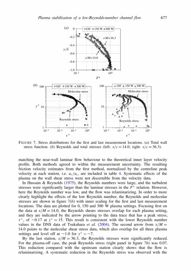
FIGURE 7. Stress distributions for the first and last measurement locations. (a) Total wallstress function. (b) Reynolds and total stresses (left: x/c= 14.0; right: x/c= 36.3).

matching the near-wall laminar flow behaviour to the theoretical inner layer velocityprofile. Both methods agreed to within the measurement uncertainty. The resultingfriction velocity estimates from the first method, normalized by the centreline peakvelocity at each station, i.e. uτ/uc, are included in table 4. Systematic effects of theplasma on the wall shear stress were not discernible from the velocity data.

In Hussain & Reynolds (1975), the Reynolds numbers were large, and the turbulentstresses were significantly larger than the laminar stresses in the F+ relation. However,here the Reynolds number was low, and the flow was relaminarizing. In order to moreclearly highlight the effects of the low Reynolds number, the Reynolds and molecularstresses are shown in figure 7(b) with inner scaling for the first and last measurementlocations. The data are plotted for 0, 150 and 300 W plasma settings. Focusing first onthe data at x/M = 14.0, the Reynolds shears stresses overlap for each plasma setting,and they are indicated by the arrow pointing to the data trace that has a peak stress,τ+, of ∼0.17 at y+ = 15. This result is consistent with the lower Reynolds numbervalues in the DNS data of Tsukahara et al. (2004). The second arrow from x/M =14.0 points to the molecular shear stress data, which also overlap for all three plasmasettings and level off at ∼1.0 for y+ <∼7.

By the last station, x/M = 36.3, the Reynolds stresses were significantly reduced.For the plasma-off case, the peak Reynolds stress (right panel in figure 7b) was 0.07.This reduction compared with the upstream station clearly shows that the flow isrelaminarizing. A systematic reduction in the Reynolds stress was observed with the


plasma on, where the peak values were 0.04 and 0.02 for the 150 W and 300 Wpower settings, respectively. This systematic reduction with RF power setting isdiscussed in § 4. Moreover, the downstream peak moved up slightly to y+ = 20. Thesecond arrow from the x/M= 36.3 points to the molecular stress results. The data forall three plasma settings overlap, and the profiles are slightly fuller than the upstreamprofiles. The effect of the plasma on the Reynolds number is listed in table 1, whereReτ was nearly constant in the duct downstream of the plasma location.

The axial velocity profiles are plotted in figure 8. The magnitude of the transversevelocity was less than 0.2 m s−1 at all measurement locations. Therefore, those dataare not shown. The axial velocity plots with outer scaling are shown in figure 8(a).The corresponding inner variable scaled profiles are shown in figure 8(b) for the lowersurface. The turbulent boundary layer laminar sublayer and logarithmic curves areindicated on each plot via the solid lines. The theoretical laminar solution for channelflow is also shown as dashed lines. The data in figures 8(a) and 8(b) show that thevelocity profile systematically changed shape from one resembling what is expectedfor a turbulent channel flow at x/M = 14.0 to a more parabolic profile, which isindicative of laminar flow, by x/M = 36.3. This relaminarization was expected asthe Reynolds number, Reτ = 49, was below the threshold required to sustain fullydeveloped turbulent flow (Narayanan 1968).

The data in figure 8 also show a slight asymmetry, where the peak velocity wasconsistently located at y/δ ∼ −0.1. This asymmetry was most likely the result ofslight manufacturing defects within the facility. In addition, the data below y+∼ 10 atx/M= 18.6 and 26.9 showed systematic departures from the theoretical curves, wherethe velocities measured were higher than expected. This region corresponds to thehigh-temperature plasma streaks shown in figure 4(a). However, high-temperatureeffects were investigated and could not be correlated with the observed largervelocities. Instead, plasma-induced flow acceleration or sheath effects may haveinfluenced these data.

3.4. Turbulence measurementsThe axial and transverse turbulence intensities are shown in figure 9(a) and theReynolds stress plots are presented in figure 9(b). The data in figure 9 are plottedfor the same locations as in figure 8. The data are presented with inner scaling;that is, ( )′+ = ( )′rms/uτ and τ+xy = −u′v′/u2

τ , where u′ and v′ are the axial andtransverse velocity fluctuations about the mean, respectively. Although the profilesare representative of a fully developed channel flow, the turbulence intensities andReynolds shear stress peak values were significantly lower than typically seen forhigh Reynolds number flows. This is consistent with the lower Reynolds numberDNS data of Tsukahara et al. (2004).

Looking at the axial trends, the turbulence intensity and Reynolds stress datashow systematic reductions in the shear layer regions for the plasma-off case. Thesedata are consistent with the velocity results and further suggest that the viscousshear production is insufficient to maintain the fully developed turbulent flow. Theplasma-off axial turbulence intensities were reduced by 10–15 % by the last station.With the plasma on, the reductions were 30 and 40 % for the 150 and 300 W cases,respectively. The transverse stresses were reduced by 30 % by the last station, andthe results were remarkably independent of the plasma setting, with the exceptionof the apparently outlying results near the upper wall at the last two stations. Theplasma-off Reynolds shear stresses were reduced by ∼60 % by the last station. With


(a)

–1.0–0.8–0.6–0.4–0.2

00.20.40.60.81.0

0 0.2 0.4 0.6 0.8 1.0

y/HOff

150 W

300 W

0

5

10

15

20

25

1 10 100

u+

Off

150 W

300 W

u+ = y+

u+ = 2.5lny+ + 5.5

Laminartheory

(b)

–1.0–0.8–0.6–0.4–0.2

00.2

0

0

0.40.60.81.0

0 0.2 0.4 0.6 0.8 1.0

y/H

0

5

10

15

20

25

1 10 100

u+

(c)

–1.0–0.8–0.6–0.4–0.2

0.20.40.60.81.0

0 0.2 0.4 0.6 0.8 1.0

y/H

0

5

10

15

20

25

1 10 100

u+

(d)

–1.0–0.8–0.6–0.4–0.2

0.20.40.60.81.0

0 0.2 0.4 0.6 0.8 1.0

y/H

u/uc

0

5

10

15

20

25

1 10 100

u+

y+

FIGURE 8. Mean velocity measurements with outer scaling (left) and inner scaling (right).(a) x/M = 14.0. (b) x/M = 18.6. (c) x/M = 26.9. (d) x/M = 36.3.


–1.0–0.8–0.6–0.4–0.2

00.20.40.60.81.0

–1.0–0.8–0.6–0.4–0.2

00.20.40.60.81.0

0 0.5 1.0 1.5 2.0

u, Off u, 150 W u, 300 W , Off , 150 W , 300 W

–0.3 –0.2 –0.1 0 0.1 0.2 0.3

Off 150 W 300 W

y/H

(a)

–1.0–0.8–0.6–0.4–0.2

0.20

0.40.60.81.0

–1.0–0.8–0.6–0.4–0.2

0

0 0

0.20.40.60.81.0

0 0.5 1.0 1.5 2.0 –0.3 –0.2 –0.1 0 0.1 0.2 0.3

y/H

(b)

–1.0–0.8–0.6–0.4–0.2

0.20.40.60.81.0

–1.0–0.8–0.6–0.4–0.2

0.20.40.60.81.0

0 0.5 1.0 1.5 2.0 –0.3 –0.2 –0.1 0 0.1 0.2 0.3

y/H

(c)

0 0

–1.0–0.8–0.6–0.4–0.2

0.20.40.60.81.0

–1.0–0.8–0.6–0.4–0.2

0.20.40.60.81.0

0 0.5 1.0 1.5 2.0 –0.3 –0.2 –0.1 0 0.1 0.2 0.3

y/H

(d)

FIGURE 9. Turbulence results: Turbulence intensity (left); Reynolds shear stress (right).(a) x/M = 14.0. (b) x/M = 18.6. (c) x/M = 26.9. (d) x/M = 36.3.


–0.4–1.0–0.8–0.6–0.4–0.2

–0.2 0

00.20.40.60.81.0

0.2 0.4

x/M=14.0

x/M=36.3

Off

150 W

300 W

Cxy

FIGURE 10. The Reynolds shear stress correlation coefficient.

the plasma on, the turbulence reduction was enhanced; the reductions were 75 and85 % for the 150 and 300 W cases, respectively.

Similarly to the velocity data, the turbulence data show a slight asymmetry, wherethe minimum axial turbulence intensity and the zero crossing of the Reynolds stresswere located near y/H =−0.1. The data also show a slight asymmetry in turbulencelevels in the shear layer regions. For example, at x/M=14.0, the peak axial turbulenceintensity along the upper surface was approximately 5 % higher than that along thebottom surface. Because the scaling in figure 9 masks the trends along the zero-shearregion, these data are described in § 4.

Examination of the evolution of the Reynolds shear stress correlation coefficientprovides insight into the underlying structure. Hence, Cxy = τxy/(−τxx)

1/2(−τyy)1/2

is plotted in figure 10 for the upstream (x/M = 14.0) and final (x/M = 36.3)stations. Upstream of the plasma, the correlation was independent of the plasmasetting. The upstream data overlap for each plasma setting. Comparison of thedownstream plasma-off data with the upstream data shows that the axial and transversevelocity fluctuations became less correlated; the magnitude of Cxy decreased fromapproximately 0.3 to 0.2. This reduction suggests that the large-scale structures thatare responsible for most of the Reynolds stresses were disintegrating as the flowrelaminarized. Application of the plasma significantly enhanced this process, as themagnitude of Cxy systematically decreased as the plasma power was increased.

4. DiscussionA principal observation from § 3 is that the plasma had a significant and systematic

effect on the axial evolution of the mean flow and turbulence. In this section, wequantify the axial flow evolution and discuss proposed mechanisms for the observedresponse of the turbulence.

4.1. Mean flow evolutionAn integral conservation law balance following Shapiro (1953) was performed toestablish a relation between the mean velocity, translational temperature and pressurefield. The goal was to connect the fluid dynamic kinematics and pressure field to thethermal non-equilibrium heat release.

First, in the limit of low Mach numbers, the one-dimensional Rayleigh theoryreduces to a direct scaling between the temperature and velocity ratios, whereTon/Toff ≈um,on/um,off . The subscripts on and off denote plasma on and off, respectively.


The Rayleigh heat addition is given by QR ≈ m Cp(Ton − Toff ). Using this, thetemperature and the heat addition were estimated from the mean PIV velocity data.The Rayleigh temperature estimates (square symbols) are compared with the PLIFmeasurements for the 300 W test conditions in figure 6. The PLIF results arenominally 4.0 % higher, with the exception of the anomalous point at x/M = 30.6.The difference is within the combined uncertainties for the two measurements. TheRayleigh heat addition for the 300 W test condition (labelled QR) is also shown infigure 6. The larger triangles were based on the PLIF temperature measurements, andthe small triangles were based on the velocity data. The solid line is an estimatebased on the temperature estimates from the vibrational decay exponential fits, asdescribed earlier. These data suggest that approximately 40 % of the RF power wasreleased into the flow as translational and rotational energy.

Second, the axial pressure gradient was estimated via an integral momentumbalance, with the resulting expression written in terms of the Clauser equilibriumpressure gradient parameter, β = (δ∗/τw)(dp/dx). In this expression, δ∗ is thedisplacement thickness, τw is the wall shear stress and dp/dx is the axial pressuregradient. The resulting expression is given by

β =−δ∗ ( 12 u−2

τ du2m/dx+ P/A

). (4.1)

In this relation, P is the perimeter of the test section and A is the correspondingcross-sectional area. The results of this expression were evaluated with the datain table 4 and are included in table 5. Hussain & Reynolds (1975) show that forfully developed flow, dp/dx = −τw/δ, which reduces to β = −δ∗/δ. It is expectedthat this expression will be applicable to the plasma-off case as the wall divergencewas selected to produce a constant mean velocity along the duct; see table 4. Thedisplacement thickness is included in table 5 for comparison. The computed pressuregradient parameter, for the plasma-off case, matches well with the correspondingdisplacement thicknesses. The differences are attributed to the relaminarizing velocityprofile on moving in the axial direction; see the progression in figure 8(a). Theprofile shape change is quantified by the shape factor (H), which is the ratio of thedisplacement to momentum thickness (i.e. H= δ∗/θ ). The shape factors are also listedin table 5.

When the plasma was in operation, the flow experienced a relatively strongfavourable pressure gradient across the electrodes, where the favourable strengthβ systematically increased to −0.5 and −0.7 for RF power settings of 150 W and300 W, respectively. One possibility for this effect is thermal heating of the facilitywalls near the electrode, which would result in increased displacement of the flownear the surface, creating a nozzle effect with flow acceleration. The presence of hotstreaks in figure 4(a), located near y+ ∼ 12 (or 20 % of δ), suggests the existence ofa thermal layer. Similarly, Rayleigh heating would also contribute.

The acceleration parameter, K = (ν/u2m)dum/dx, is often used to characterize the

onset of relaminarization (Patel & Head 1968). For the present study, K peaked onmoving across plasma at 2 × 10−5 and 4 × 10−5 for 150 and 300 W, respectively.These values are about an order of magnitude higher than the relaminarization onsetcriteria given in Narasimha & Sreenivasan (1979). The relatively large changes inthis parameter predict strong effects from the RF plasma. On the other hand, thePatel (1965) non-dimensionalized pressure gradient α0 = (ν/ρu3

τ )(∂p/∂x) values werealso found to be negligibly small compared with the criteria for relaminarization(Narasimha & Sreenivasan 1979).


Pressure gradient parameter (β)

x/M 16.3 20.1 24.2 29.2Off −0.26 −0.24 −0.26 −0.32150 W −0.48 −0.20 −0.38 −0.27300 W −0.70 −0.22 −0.38 −0.25

Displacement thickness (δ∗/δ)

x/M 14.0 18.6 21.5 26.9 36.3Off 0.21 0.22 0.24 0.24 0.28150 W 0.22 0.20 0.22 0.23 0.28300 W 0.22 0.19 0.22 0.22 0.28

Shape factor (H)

x/M 14.0 18.6 21.5 26.9 36.3Off 2.35 2.41 2.47 2.43 2.59150 W 2.45 2.08 2.47 2.35 2.51300 W 2.45 1.98 2.41 2.36 2.50

TABLE 5. Shear layer parameters.

4.2. Zero-shear turbulence evolutionTo better isolate the effects of the electronic excitation and subsequent vibrationalrelaxation on the axial evolution of the turbulence in the zero-shear region of the duct(y/δ∼−0.1), the normal stresses and turbulent kinetic energy, with outer scaling, areplotted in figure 11 versus the non-dimensional advection time through the duct. Thedata are normalized such that t1 corresponds to x/M = 21.5. This value was selectedas it serves as an approximate dividing line between two distinct regions in the flow.The first is the near field, where the plasma and grid effects were the prominentprocesses, and the second is the far field, where the turbulence was characterized bynearly isotropic decay and the vibrational relaxation was a significant non-equilibriumprocess. The plasma was located at t/t1 = 0.74 with this scaling. The time scale wascomputed at each measurement location using the average peak velocity betweensuccessive measurement locations to account for the acceleration due to the plasma.

The transverse (v′) data in figure 11 appear to have been unaffected by the plasmasetting; this is consistent with Sreenivasan (1982). Moreover, one should recall that thetransverse velocity fluctuation intensity was nominally independent of the transversecoordinate at each axial location, which indicates a constant static pressure across theduct. This lack of dependence of the transverse velocity on the plasma setting hasimplications towards explaining the underlying processes. Specifically, the transverseturbulence shear stress (τyy) transport equation can be written as

Dτ Tyy/Dt≈ 2RC−1

v (ϑTy,y − ρ〈e′v′,y〉)+ 2

3ρε, (4.2)

where simplifications for nearly isotropic decay were performed (Wilcox 2000) and thepressure fluctuations associated with the pressure–strain redistribution were expressedin terms of energy fluctuations assuming a thermally perfect gas and neglectingdensity fluctuations. In (4.2), R is the gas constant for air, Cv is the specific heat atconstant volume for air, e′ is the translational energy and ϑT

i = ρ〈e′u′i〉 is the energyflux (Bowersox 2009). For the plasma-off case, the first term on the right-hand


0.50

0.001

0.002

0.003

0.004

0.005

1.0 1.5 2.0

Off

150 W

300 W

k

u

t/t1

FIGURE 11. Turbulence in the zero-shear region (y/H=−0.1). The dashed line indicatesthe plasma position.

side is expected to be negligible due to transverse symmetry. The second termwas either negligible or unaffected by the plasma. Since the transverse fluctuationswere unaffected by the plasma, these terms apparently remained negligible for therange of plasma conditions tested here. It is also reasonable to presume that thevibrational excitation impacted the molecular viscosity and hence the dissipation in(4.2). However, it is expected that the populations of vibrationally excited moleculeswould be small enough (∼12 % for 300 W) for this effect to probably be negligible.The observed lack of dependence on plasma setting for the transverse data tends toconfirm this assertion.

Unlike the transverse component, the axial Reynolds stress data show significantvariation with plasma setting. The turbulence levels upstream of the plasma wereslightly reduced while the plasma was operating. It should be recalled that theupstream mean velocity was also reduced, which is believed to be the result of thethermal blockage. The reduced turbulence may have resulted from the stabilizingeffects of the wall heating (Nicholl 1970) from the electrodes moving upstreamthrough conduction. Just downstream of the plasma, the turbulence levels appearedto rise to values similar to those for the plasma off, and then decayed more rapidly.Examination of the axial transport equation provides additional insight into theprocesses leading to the trends in figure 11. The axial Reynolds stress transportequation, following the discussion with respect to (4.2), is written as

Dτ Txx/Dt∼−2τ T

xxu,x + 2RC−1v (ϑ

Tx,x − ρ〈e′u′,x〉)+ 2

3ρε. (4.3)

The assumption that the dissipation for the axial stress is also independent of theplasma setting suggests that the first and second terms on the right-hand side of(4.3) play important roles in the observed trend. The first term is the productionresulting from the axial acceleration and the second results from the pressure strain;see the discussion of (4.2). For the first term, the positive axial velocity gradientsare stabilizing, which agrees with the reduced axial stresses observed in figure 11.The second term is related to the molecular energy exchange process, where thedilatational part of this term is likely to be negligible, as was observed for (4.2).

To help to illustrate the energy exchange process, the translational energy fluxtransport equation, derived from the momentum and energy equations, was examined.To simplify the analysis, the pressure-scrambling, diffusion and dissipation terms were


omitted on an ad hoc basis; see Bowersox (2009). The resulting axial energy fluxequation is given by

DϑTx /Dt∼ τ T

xxe,x − ϑTx u,x + ρq′u′. (4.4)

The first two terms on the right-hand side of (4.4) represent production and the thirdterm denotes the molecular exchange process between the energy pools. For flowsthat are close to adiabatic, ϑT

x < 0 (Chen & Blackwelder 1978). Assuming this tobe the case here, the first term is destabilizing (i.e. it makes ϑT

x more negative). Thesecond is stabilizing as the flow is accelerating and the axial stress is negative. For theexchange term, a Landau–Teller (1936) approximation was employed given that thevibrational excitation was limited to the first level of nitrogen in the downstream decayregion of the flow. With this, the third term reduces to ρq′u′∼−(ϑT(vib)

i −ϑT(vib)i,eq )/τvib,

where τ−1vib ≈ um/Lvib. Taking Lvib as the characteristic relaxation length from figure 6

(Lvib/M∼ 75 for both plasma-on cases), and expanding the material derivative in (4.4)as DϑT

x /Dt ≈ ϑTx,t + umϑ

Tx,x, where the average bulk convection velocity um is taken

here as a constant, results in the following approximation for the axial gradient ofthe energy flux:

ϑTx,x ∼ τ T

xxe,x/um − ϑTx u,x/um −1ϑT(vib)

x,x /Lvib − ϑTx,t/um. (4.5)

With this relation, and assuming that the flow is statistically steady, (4.3) reduces to

Dτ Txx/Dt∼ 2τ T

xx(−u,x + RT,x/um)− 2RC−1v (ϑ

Tx u,x/um +1ϑT(vib)

x,x /Lvib)+ 23ρε. (4.6)

Term-by-term assessment of the signs indicates that the present velocity gradientis stabilizing in both appearances (recall that τxx < 0); the thermal gradient, whichresults from the vibrational decay, is destabilizing; the vibrational exchange term isuncertain as the sign on the vibrational energy flux is unknown, and any increase inthe dissipation is stabilizing. The response of the turbulence shown in figure 11 isthe result of the net balance of the mechanical and thermal non-equilibrium terms inthe transport equation, which evidently was stabilizing for the present study.

The far-field fluctuation amplitude data appear to approach a power law decay trendnear the third measurement station. Thus, the far-field turbulent kinetic energy, k =(u′2+ v′2)/2 for t/t1> 1 was fitted, via least squares, with the expected isotropic decaypower law k/k1 = (t/t1)

−1/n, which is similar to the approach described by Huang& Leonard (1994). The resulting values for n were 1.0 and 0.8 for the plasma-offand plasma-on cases, respectively. The plasma-off values are in good agreement withBatchelor & Townsend (1948). This agreement is considered fortuitous given that, inthe present small duct, the anisotropy was significant, e.g. u′2/v′2 ≈ 2.5.

In the near field, the nitrogen molecules undergo significant electronic excitationand subsequent relaxation over an axial span of ∼1 cm. This, in turn, results inrapid energy exchange into translation, rotation and vibration. These energy gradientsprovide additional mechanisms to produce energy fluxes. The net effect of thesemolecular processes may have been significant in the near-field (t/t1 < 1) turbulencestabilization. Again, exact enumeration of the relative magnitudes of the terms is notpossible as the role of the molecular exchange is uncertain.

4.3. Shear layer turbulence evolutionA pronounced feature in figure 9 is the reduced levels of the peak axial intensitiesand Reynolds shear stresses in the shear layer region, when the plasma was on. The


100 0

0.04

0.08

0.12

0.16

0.20

0.24

0.4

0.8

1.2

1.6

2.0

20 30 40 10 20 30 40

u

x/M x/M

Off

150 W

300 W

(a) (b)

FIGURE 12. The axial evolution of shear layer turbulence; the dashed vertical lineindicates the plasma position. (a) Turbulence intensity peak. (b) Reynolds stress peak.

locations of the peak levels varied from y/δ=−0.8 to −0.7 on moving from the firstto last measurement station. The corresponding viscous scaled coordinates are y+ =11 and 14, respectively. To better quantify the trends, the peak values are plotted infigure 12 with inner scaling. The most prominent features in figure 12(a) are the 15and 30 % drops in axial turbulence intensity across the plasma for the 150 and 300 Wcases, respectively, as compared to the plasma-off case. The subsequent decay rateswere least-squares fits (lines in figure 11a) with a power law of a(x/M)−m, wherethe fit parameters (a,m) were (2.98,−0.22), (3.41,−0.32) and (3.79,−0.41) for theplasma-off, 150 and 300 W cases, respectively. Hence, the decay rate also increaseswith the plasma power, which is consistent with the discussion in the previous section.Moreover, the peak turbulence levels upstream of the plasma (x/M= 14.0) showed asystematic reduction as the plasma strength was increased. Similarly to the previoussection, the peak shear transverse fluctuations were apparently unaltered by the plasma.The fit parameters are given by (1.85, 0.46) for all three cases.

Referring to figure 12(b), the Reynolds stresses were reduced by 30 and 50 %across the plasma for the 150 and 300 W cases, respectively. The subsequent decayrates were also power law fitted (lines in figure 12b). The parameters (a, m) were(3.84,−1.12), (4.54,−1.31) and (12.0,−1.73) for the plasma-off, 150 W and 300 Wcases, respectively, which also shows that the decay increased with increasing plasmapower. As with the axial fluctuations, the upstream Reynolds stress levels appearedto have been influenced by the plasma setting.

Mathematically, the transport equation description is significantly more complicatedin the shear layer region. For example, the Reynolds stress transport equation can bewritten as

Dτ Txy

Dt≈−τ T

yyu,y − τ Txyu,x − ρ(p′u′,y + p′v′,x)+

RCv

(ϑTx,y + ϑT

y,x), (4.7)

where molecular diffusion and dissipation were omitted for clarity. Referring to thisexpression, the plasma changed the principal production, i.e. the first term on theright-hand side, by altering the velocity gradients (see figure 8b). It should be recalledthat the transverse stress was unaffected. The second (extra) production term was alsosignificant due to the axial acceleration. Bradshaw (1973) points out that pressure


gradients alter the turbulence by an order of magnitude more than would be expectedby the magnitude of the extra production (e.g. the second term). The pressure–strainterm can be rewritten in terms of the energy fluctuations via the thermal equationof state. Hence, this term provides another mechanism for the plasma to alter theunderlying state of the turbulence. Similarly, the pressure-diffusion, i.e. the last term in(4.7), which was expressed in terms of the energy fluctuations via the thermal equationof state, also provides a mechanism for the plasma to alter the Reynolds shear stress.Although we cannot unravel the intricate processes, the net effect of the plasma issignificant stabilization across the flow.

5. Conclusions

An experimental study was performed to characterize the stabilizing effects ofRF plasma heating and thermal non-equilibrium on the statistical properties of alow-Reynolds-number (Reτ = 45) relaminarizing channel flow. Tests were conductedutilizing 0, 150 and 300 W RF plasma power settings. The mean and turbulentflow properties were quantified using PIV, two-line planar laser induced fluorescence,dual-pump broadband BOXCARS, as well as broadband and high-resolution emissionspectroscopy.

The RF plasma produced a two-temperature non-equilibrium flow, where the N2 wasvibrationally excited to 1240 and 1550 K for the 150 and 300 W settings, respectively.Oxygen was not significantly excited, and the rotational and translational temperatureswere slightly elevated above room temperature. The following quantitative observationswere drawn concerning the effects of the present RF plasma on the turbulence flowproperties.

(i) The Reynolds axial stresses dropped by 15 and 30 % across the plasma for the150 and 300 W cases, respectively, compared with the plasma-off case. Thesubsequent decays followed a power law form, where the decay rate increasedwith the plasma power. By the last station, the axial turbulence intensities werereduced by 15, 30 and 40 % for the 0, 150 and 300 W cases, respectively.

(ii) The transverse fluctuations were apparently unaltered by the plasma. Thedownstream decay agreed with a power law fit.

(iii) The Reynolds stresses were reduced by 30 and 50 % across the plasma for the150 and 300 W cases, respectively, and subsequently fitted with a power law. Bythe last station, the Reynolds shear stresses were reduced by 60, 75 and 85 % forthe 0, 150 and 300 W cases, respectively.

(iv) The reductions in the shear stress correlation coefficient were 30, 50 and 70 % forthe 0, 150 and 300 W cases, respectively. These data suggest that the large-scalestructures responsible for most of the Reynolds stresses were disintegrating.

(v) The plasma enhanced the turbulence decay in the zero-shear region as a result offlow acceleration, where the power law decay t−1/n exponential factor decreasedfrom n≈ 1.0 to 0.8.

Qualitatively, the RF plasma significantly stabilized the turbulence in both the shearand zero-shear regions of the flow. Integral conservation law balance and second-ordertransport analyses demonstrated that the plasma induced thermal non-equilibrium,thermal heating, flow acceleration and wall heating. All of these processes have thepotential to directly affect the underlying state of the turbulence.


AcknowledgementsThis work was sponsored (in part) by the Air Force Office of Scientific Research,

USAF under grant FA9550-04-1-0425. The views and conclusions contained hereinare those of the authors and should not be interpreted as necessarily representing theofficial policies or endorsements, either expressed or implied, of the Air Force Officeof Scientific Research or the US government.

REFERENCES

ALEKSANDROV, A. F., VIDIAKIN, N. G., LAKUTIN, V. A., SKVORTSOV, M. G. & TIMOFEEV, I. B.1986 A possible mechanism for interaction of a shock wave with a decaying laser plasma inair. Sov. Phys. Tech. Phys. 31 (4), 468–469.

ALLEN, J. 1992 Probe theory – the orbital motion approach. Phys. Scr. 45 (5), 497–503.ARNETTE, S., SAMIMY, M. & ELLIOTT, G. 1998 The effects of expansion on the turbulence structure

of compressible boundary layers. J. Fluid Mech. 367, 67–105.BARNES, M., KELLER, J., FORSTER, J., O’NEIL, J. & COUTLAS, D. 1992 Transport of dust particles

in glow-discharge plasmas. Phys. Rev. Lett. 68, 313–316.BASS, H. 1981 Absorption of sound by air: high temperature predictions. J. Acoust. Soc. Am. 69

(1), 124–138.BATCHELOR, G. & TOWNSEND, A. 1948 Decay of isotropic turbulence in the initial period. Proc.

R. Soc. Lond. A 193, 539–558.BENEDICT, L. & GOULD, R. 1996 Towards better uncertainty estimates for turbulence statistics. Exp.

Fluids 22, 129–136.BISKAMP, D. 1993 Nonlinear Magnetohydrodynamics. Cambridge University Press.BISKAMP, D. 2000 Magnetic Reconnection in Plasmas. Cambridge University Press.BISKAMP, D. 2003 Magnetohydrodynamic Turbulence. Cambridge University Press.BOEUF, J. & PUNSET, C. 1999 Physics and modeling of dusty plasma. In Dusty Plasmas (ed.

A. Bouchoule), chap. 1. John Wiley and Sons.BOWERSOX, R. D. W. 2009 Extension of equilibrium turbulent heat flux models to high-speed shear

flows. J. Fluid Mech. 633, 61–70.BRADSHAW, P. 1969 The analogy between streamline curvature and buoyancy in turbulent shear

flow. J. Fluid Mech. 36, 177–191.BRADSHAW, P. 1973 The effect of streamline curvature on turbulent flow, AGARD-AG-169, NATO

Science and Technology Organization.BRENNAN, M., ALLE, D., EURIPIDES, P., BUCKMAN, S. & BRUNGER, M. 1992 Elastic electron

scattering and rovibrational excitation of N2 at low incident energies. J. Phys. B: At. Mol.Opt. Phys. 25, 2669–2682.

CATTOLICA, R. 1981 OH rotational temperature from two-line laser-excited fluorescence. Appl. Opt.20, 1156–1166.

CHEN, C. & BLACKWELDER, R. 1978 Large-scale motion in a turbulent boundary layer: a studyusing temperature contamination. J. Fluid Mech. 89, 1–31.

CHEN, Q., CHEN, S. & EYINK, G. 2003 The joint cascade of energy and helicity in three-dimensionalturbulence. Phys. Fluids 15 (2), 361–374.

CHO, J. 2011 Magnetic helicity conservation and inverse energy cascade in electronmagnetohydrodynamic wavepackets. Phys. Rev. Lett. 106, 191104-1–191104-4.

CHRISTENSEN, K. & ADRIAN, R. 2001 Statistical evidence of hairpin vortex packets in wallturbulence. J. Fluid Mech. 431, 433–443.

DUSSAUGE, J. P. & GAVIGLIO, J. 1987 The rapid expansion of a supersonic turbulent flow: role ofbulk dilatation. J. Fluid Mech. 174, 81–112.

EKOTO, I., BOWERSOX, R. D. W., BEUTNER, T. & GOSS, L. 2009 Response of supersonic turbulentboundary layers to local and global mechanical distortions. J. Fluid Mech. 630, 225–265.

EVTYUKHIN, N. V., MARGOLIN, A. D. & SHMELEV, V. M. 1986 On the nature of shock waveacceleration in glow discharge plasma. Sov. J. Chem. Phys. 3, 2080–2089.


FALGARONE, E. & PASSOT, T. (Eds) 2003 Turbulence and Magnetic Field in Astrophysics, Lect.Notes Physics. Springer, Berlin.

FUJII, K. & HORNUNG, H. 2003 Experimental investigation of high-enthalpy effects on attachment-lineboundary-layer transition. AIAA J. 41 (7), 1282–1291.

GALTIER, S. & BHATTACHARJEE, A. 2003 Anisotropic weak whistler wave turbulence in electronmagnetohydrodynamics. Phys. Plasmas 10 (8), 3065–3076.

HANSON, R. K. 1988 Planar laser-induced fluorescence imaging. J. Quant. Spectrosc. Radiat. Transfer40, 343–362.

HUANG, M.-J. & LEONARD, A. 1994 Power-law decay of homogeneous turbulence at low Reynoldsnumbers. Phys. Fluids 6, 3765–3775.

HUSSAIN, A. & REYNOLDS, W. 1975 Measurement in a fully developed channel flow. Trans. ASME,J. Fluids Engrs 97 (4), 68–78.

IONIKH, Y., CHERNYSHEVA, N., MESHCHANOV, A., YALIN, A. & MILES, R. 1999 Direct evidenceor thermal mechanism of plasma influence on shock wave propagation. Phys. Lett. A 259,387–392.

ITIKAWA, Y., HAYASHI, M., ICHIMURA, A., ONDA, K., SAKIMOTO, K., TAKAYANAGI, K.,NAKAMURA, M., NISHIMURA, H. & TAKAYANAGI, T. 1986 Cross-sections for collisions ofelectrons and photons with nitrogen molecules. J. Phys. Chem. Ref. Data 15 (3), 985–1010.

ITIKAWA, Y., ICHIMARU, A., ONDA, K., SAKIMOTO, K., TAKAYANAGI, K., HATANO, Y.,HAYASHI, M., NISHIMURA, H. & TSURUBUCHI, S. 1989 Cross-sections for collisions ofelectrons and photons with oxygen molecules. J. Phys. Chem. Ref. Data 18 (9), 23–42.

KIM, H., KLINE, S. & REYNOLDS, W. 1971 The production of turbulence near a smooth wall in aturbulent boundary layer. J. Fluid Mech. 50, 133–160.

KLIMOV, A., KOBLOV, A., MISHIN, G., SEROV, Y. & YAVOR, I. 1982 Shock wave propagation in aglow discharge. Sov. Phys. Tech. Phys. 8 (4), 192–194.

KLINE, S., REYNOLDS, W., SCHRAUB, F. & RUNSTADLER, P. 1967 The structure of turbulentboundary layers. J. Fluid Mech. 30, 741–773.

LANDAU, L. & TELLER, E. 1936 Zur theorie der schalldispersion. Phys. Z. Sowjetunion 10 (1), 34.LAUNDER, B., REECE, G. & RODI, W. 1975 Progress in the development of a Reynolds-stress

turbulence closure. J. Fluid Mech. 68 (3), 537–566.LEYVA, I., JEWELL, J., LAURENCE, S., HORNUNG, H. & SHEPHERD, J. 2009 On the impact of

injection schemes on transition in hypersonic boundary layers, AIAA Paper 2009-7204.LOTH, E. 2008 Compressibility and rarefaction effects on drag of a spherical particle. AIAA J. 46,

2219–2228.LUCHT, R. P. 1987 Three-laser coherent anti-Stokes Raman scattering measurements of two species.

Opt. Lett. 12 (2), 78–80.LUKER, J., BOWERSOX, R. D. W. & BUTER, T. 2000 Influence of a curvature driven favorable

pressure gradient on a supersonic turbulent boundary layer. AIAA J. 38 (8), 1351–1359.MACHERET, S. O., IONIKH, Y. Z., CHERNYSHEVA, N. V., YALIN, A. P., MARTINELLI, L. &

MILES, R. B. 2001 Shock wave propagation and dispersion in glow discharge plasmas. Phys.Fluids 13 (9), 2693–2705.

MADEN, I., MADUTA, R., KRIEGSEIS, J., JAKIRLIC, S., SCHWARZ, C., GRUNDMANN, S. &TROPEA, C. 2013 Experimental and computational study of the flow induced by a plasma.Intl J. Heat Fluid Flow 41, 80–89.

MARTIN, M. P. & CANDLER, G. V. 1998 Effect of chemical reactions on decaying isotropicturbulence. Phys. Fluids 10 (7), 1715–1724.

MATSOUKAS, T. & RUSSELL, M. 1995 Particle charging in low-pressure plasmas. J. Appl. Phys. 77,4285–4292.

MCMILLIN, B., PALMER, J. & HANSON, R. 1993 Temporally resolved, two-line fluorescence imagingof NO temperature in a transverse jet in a supersonic cross flow. Appl. Opt. 32, 7532–7545.

MENON, R. & LAI, W. 1991 Key considerations in the selection of seed particles for LDVmeasurements. In 4th Int. Conf. on Laser Anemometry, TSI Inc.

MERRIMAN, S., PLOENJES, E., PALM, P. & ADAMOVICH, I. 2001 Shock wave control bynonequilibrium plasmas in cold supersonic gas flows. AIAA J. 39 (8), 1547–1552.


MONTELLO, A., NISHIHARA, M., RICH, W., ADAMOVICH, I. & LEMPERT, W. 2012 Nitrogenvibrational population measurements in the plenum of a hypersonic wind tunnel. AIAA J.50, 1368–1376.

MOTT-SMITH, H. & LANGMUIR, I. 1926 The theory of collectors in gaseous discharges. Phys. Rev.28 (4), 727–763.

NAKANISHI, R., MAMORI, H. & FUKAGATA, K. 2012 Relaminarization of turbulent channel flowusing wave-like wall deformations. Intl J. Heat Fluid Flow 35, 152–159.

NARASIMHA, R. & SREENIVASAN, K. R. 1979 Relaminarization of fluid flows. Adv. Appl. Mech.19, 221–309.

NARAYANAN, B. 1968 An experimental study of reverse transition in two-dimensional channel flow.J. Fluid Mech. 31 (part 3), 609–623.

NICHOLL, C. 1970 Some dynamical effects of heat on a boundary layer. J. Fluid Mech. 40 (2),361–384.

OSIPOV, A., UVAROV, A. & VINNICHENKO, N. 2006 Influence of the initial vibrationally non-equilibrium state of a medium on the structure of von Karman vortex sheet. Phys. Fluids 18,1–7.

PALM, P., MEYER, R., PLONJES, E., RICH, J. & ADAMOVICH, I. 2003 Nonequilibrium radio frequencydischarge plasma effect on conical shock wave: M = 2.5 flow. AIAA J. 41 (3), 465–469.

PALMER, R. 1989 The CARSFIT computer code for calculating coherent anti-Stokes Raman spectra:user and programmer information, Sandia Report SAND89-8206, Sandia National Laboratories,Livermore, CA.

PANTON, R. 1997 Self-Sustaining Mechanisms of Wall Turbulence. Computational MechanicsPublications.

PATEL, V. 1965 Calibration of the Preston tube and limitations on its use in pressure gradients.J. Fluid Mech. 23, 185–208.

PATEL, V. & HEAD, M. 1968 Reversion of turbulent to laminar flow. J. Fluid Mech. 34 (2), 371–392.RAIZER, Y. 1997 Gas Discharge Physics. Springer.ROBINSON, S. 1991 Coherent motions in the turbulent boundary layer. Annu. Rev. Fluid Mech. 23,

601–639.SCHOPPA, W. & HUSSAIN, F. 2002 Coherent structure generation in near-wall turbulence. J. Fluid

Mech. 453, 57–108.SHAPIRO, A. 1953 The Dynamics and Thermodynamics of Compressible Flow. vol. 1. chap. 8.

pp. 219–260. John Wiley & Sons.SHUKLA, P. & MAMUN, A. 2002 Introduction to Dusty Plasma. Institute of Physics Publishing.SPINA, E. F., SMITS, A. J. & ROBINSON, S. 1994 The physics of supersonic turbulent boundary

layers. Annu. Rev. Fluid Mech. 26, 287–319.SREENIVASAN, K. R. 1982 Review article laminarescent, relaminarizing and retransitional flow. Acta

Mechanica 44, 1–48.STANFIELD, S. A., JAMES MENART, DEJOSEPH. C. JR, KIMMEL, R. L. & HAYES, J. R. 2009

Rotational and vibrational temperature distributions for a dielectric barrier discharge in air.AIAA J. 47 (5), 1107–1115.

THEODORSEN, T. 1952 Mechanism of turbulence, Proc. 2nd Midwestern Conf. Fluid Mechanics,Ohio State University, Columbus, Ohio, pp. 1–19.

TICHENOR, N., HUMBLE, R. & BOWERSOX, R. D. W. 2013 Response of hypersonic turbulentboundary layer to favorable pressure gradients. J. Fluid Mech. 722, 187–213.

TREVISAN, C., HOUFEK, K., ZHANG, Z., OREL, A., MCCURDY, C. & RESCIGNO, R. 2005 Nonlocalmodel of dissociative electron attachment and vibrational excitation of NO. Phys. Rev. A 71,052714.

TSUKAHARA, T., SEKI, Y., KAWAMURA, H. & TOCHIO, D. 2004 DNS of turbulent channel flowwith very low Reynolds numbers. In Comp. Mech., WCCM VI, APCOM’04 Beijing, China,Sept. 5–10, Tsinghua University Press & Springer.

VEDENOV, A. A. 1968 Theory of Turbulent Plasma. London Iliffe Book Ltd.VERMA, M. K. 2004 Statistical theory of magnetohydrodynamic turbulence: recent results. Phys.

Rep. 401, 229–380.


VOINOVICH, P. A., ERSHOV, A. P., PONOMAREVA, S. E. & SHIBKOV, V. M. 1991 Propagation ofweak shock waves in plasma of longitudinal glow discharge in air. High Temp. 29, 468–475.

WILCOX, D. 2000 Turbulence Modeling for CFD. DCW Ind.ZHU, J.-Z., YANG, W. & ZHU, G.-Y. 2014 Purely helical absolute equilibria and chirality of (magneto)

fluid turbulence. J. Fluid Mech. 739, 479–501.

Date post:	10-Feb-2019
Category:	Documents
Upload:	ledan
View:	218 times
Download:	0 times

J. Fluid Mech. (2014), . 748, pp. doi:10.1017/jfm.2014.189 ... Flow JFM... · Radiofrequency plasma...

Documents