J. Fluid Mech. (2012), . 708, pp. 250–278. doi:10.1017/jfm ...

J. Fluid Mech. (2012), vol. 708, pp. 250–278. c� Cambridge University Press 2012 250doi:10.1017/jfm.2012.303

Forcing of oceanic mean flows by dissipating

internal tides

Nicolas Grisouard† and Oliver Bühler

Courant Institute of Mathematical Sciences, New York University, 251 Mercer Street,New York, NY 10012-1185, USA

(Received 20 January 2012; revised 29 May 2012; accepted 13 June 2012;first published online 8 August 2012)

We present a theoretical and numerical study of the effective mean force exerted onan oceanic mean flow due to the presence of small-amplitude internal waves thatare forced by the oscillatory flow of a barotropic tide over undulating topographyand are also subject to dissipation. This extends the classic lee-wave drag problemof atmospheric wave–mean interaction theory to a more complicated oceanographicsetting, because now the steady lee waves are replaced by oscillatory internal tides and,most importantly, because now the three-dimensional oceanic mean flow is defined bytime averaging over the fast tidal cycles rather than by the zonal averaging familiarfrom atmospheric theory. Although the details of our computation are quite different,we recover the main action-at-a-distance result from the atmospheric setting, namelythat the effective mean force that is felt by the mean flow is located in regions ofwave dissipation, and not necessarily near the topographic wave source. Specifically,we derive an explicit expression for the effective mean force at leading order usinga perturbation series in small wave amplitude within the framework of generalizedLagrangian-mean theory, discuss in detail the range of situations in which a strong,secularly growing mean-flow response can be expected, and then compute the effectivemean force numerically in a number of idealized examples with simple topographies.

Key words: internal waves, ocean processes, topographic effects

1. Introduction

Internal gravity waves play an essential part in the global-scale dynamics of boththe atmosphere and the oceans. This is despite their comparatively short spatial andtemporal scales, which for the most part renders them unresolvable in present-daycomputer models for the global circulation. In the atmosphere, the most importantinternal-wave effect is the wave-induced vertical transport of angular momentum andthe concomitant effective force exerted on the flow in locations where the waves breakor otherwise dissipate. Here the simplest relevant thought experiment is the lee-waveproblem, i.e. a steady wind blowing over undulating topography that generates upwardpropagating internal waves with zero absolute frequency. There is a net drag force onthe topography and, in the simplest setting of zonal averaging applied to a horizontallyhomogeneous mean flow, there is an equal-and-opposite effective force exerted on themean flow in the regions of wave dissipation. Remarkably, these lee waves are felt

† Email address for correspondence: [email protected]

Forcing of oceanic mean flows by dissipating internal tides 251

by the mean flow not where the waves are generated but only where the waves aredissipated.

The theoretical underpinnings for the computation of the effective force exertedby dissipating internal waves in the atmosphere are by now very well established(e.g. Buhler 2009, § 6), and form the basis for all parametrization schemes of sucheffects in numerical models. Basically, this classic theory works by exploiting thezonal symmetry of the assumed wind profile, which makes zonal averaging a naturalprocedure in order to distinguish the mean and disturbance parts of the flow. Clearly,a direct application of this classic theory to the ocean immediately runs into problemsbecause most oceanic currents are not zonally symmetric even to a first approximationand therefore one cannot simply apply the classic theory, which has been built aroundthis approximation. (There is one notable exception, namely the antarctic circumpolarcurrent, which encircles the globe in a manner similar to atmospheric currents.)

Little progress has been made on this problem, partly for the aforementionedtechnical reasons, but mostly because oceanographic interest in internal waves isfocused on their contribution to small-scale mixing and not on momentum transfers.Indeed, in recent years there has been significant progress in understanding therole of internal waves in the mixing processes in the deep ocean. This follows theobservational discovery some fifteen years ago that small-scale turbulence levels aregreatly elevated above regions of strong topography, a finding that has been linked toincreased internal wave activity in these regions (e.g. Polzin et al. 1997; Ledwell et al.2000). Basically, the intermittent breaking of internal waves produces patches of three-dimensional turbulence, and the small-scale turbulent mixing across these patches thencontributes to the transport of fluid particles across the stable-stratification surfacesof the ocean, which is a significant part of the functioning of the global overturningcirculation of the ocean. Several source mechanisms for such topographic internalwaves exist. For example, recently Nikurashin & Ferrari (2010a,b) have investigatedtwo-dimensional lee waves produced by geostrophic currents over periodic randomocean topography, which is similar to the atmospheric lee-wave problem and can tosome extent be studied using zonal averaging.

Probably the strongest source mechanism for topographic internal waves in theocean is provided by the barotropic tides, i.e. the relentless back-and-forth sloshing ofthe entire oceanic water column in response to lunar and solar gravitational forcing.This leads to the generation of so-called internal tides, which are topographicallygenerated internal waves with frequencies dominated by tidal frequencies. There havebeen numerous internal-tide studies in recent years (for a review see Garrett & Kunze2007), which mostly focus on the wave energy budget and its heuristic links towave-induced turbulent mixing (e.g. Muller & Buhler 2009).

In the present paper we augment these earlier internal-tide studies that were focusedon wave-induced mixing by computing the effective force exerted on the mean flowdue to wave dissipation. Basically, our aim is to use the well-studied example ofinternal tides in order to put on record a detailed wave–mean interaction probleminvolving internal waves and three-dimensional mean flows in the ocean. In keepingwith oceanographic requirements, here we define the mean flow not with zonalaveraging, but with a time average over the fast tidal oscillations. In other words,we retain the mean flow as a fully three-dimensional time-dependent flow, but weaverage over the fast time scale of the internal tides and replace the action of thewaves on the mean flow by a suitably defined effective mean force. This makes theoceanic theory slightly more difficult than its atmospheric counterpart.

252 N. Grisouard and O. Bühler

The theory is worked out in a typical scenario for internal-tide studies: a finite-depthocean modelled as a Boussinesq fluid where internal tides are first generated by tidalsloshing over localized topography and then propagate away to horizontal infinity. Justas in the atmospheric case, we will recover that the mean flow is affected by thestationary waves in regions of significant wave dissipation, but not necessarily near thetopographic source region.

In order to facilitate our study we use the simplest model for internal tides,which combines small-amplitude topography with a small-excursion assumption forthe barotropic tide, i.e. the ratio between tidally induced horizontal particle excursionsand the scale of the localized topography is assumed to be small. By using uniformrotation and stratification and no basic flow we also ignore all effects to do withshear, background turbulence, or other forms of inhomogeneity in the water column.We also use a crude and simplistic model for wave dissipation by allowing for lineardamping in the buoyancy equation. This is blatantly unrealistic for the ocean, butallows a simple handle with which to model the wave–mean interactions due towave breaking in a qualitatively correct way. In this set-up the sought effective meanforce arises at second order in wave amplitude, so we have a standard problem insmall-amplitude wave–mean interaction theory to solve, i.e. the fluid flow is studiedby a regular perturbation approach based on ascending orders in wave amplitude.We find it convenient to use the generalized Lagrangian-mean formalism to computethe leading-order mean-flow response, because in the present setting the formalismoffers the simplest mean-flow boundary conditions as well as a useful handle onthe evolution equation for the Lagrangian-mean potential vorticity (PV), central to anefficient description of the three-dimensional mean-flow dynamics.

We solve for the linear waves using a Green’s function approach similar to thatof Llewellyn Smith & Young (2002), but slightly extended to yield smooth resultsover the topography. Our main theoretical result is the expression for the nonlineareffective mean force and its curl in (4.10) and (4.11) below. The curl of this forceencapsulates the entire forcing of the second-order mean flow due to the first-orderwaves, and the vertical component of its curl captures the all-important forcing of theLagrangian-mean PV. This is the most important part of the wave–mean interactionsin this problem, because secular growth of the mean-flow response is inevitably linkedto secular growth of the PV, so the strongest interactions are those that project ontothe PV dynamics. We then illustrate the effective force structure with a number ofidealized examples with different topography shapes for which we compute the fullsolution numerically. Also, there is a superficial resemblance between our results andthose of a few other studies, most notably tidal rectification studies, so we brieflydiscuss the relationship between these theories.

The layout of the paper is as follows. The governing equations and the flow domainare described in § 2 and the linear wave solution is derived in § 3. The Lagrangian-mean equations for the second-order mean-flow response and the effective meanforce are derived in § 4. The conditions for secularly growing mean-flow responsesin various configurations are discussed in § 5 and numerical examples for differenttopography shapes are presented in § 6. Concluding comments are offered in § 7.

2. Physical and mathematical model for dissipating internal waves

2.1. Model ocean and barotropic tidal flow

The basic ocean set-up is illustrated in figure 1. We consider a standard three-dimensional Boussinesq fluid model in a domain that is unbounded in the horizontal


Top lid

U0

h0

H

xy

z

L

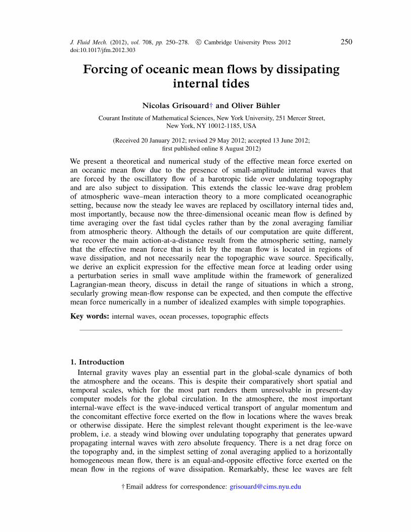
FIGURE 1. Three-dimensional set-up: a rotary barotropic tide of velocity amplitude U0 alongits major axis and γ U0 along its minor axis flows over a topography of height h0 and typicalslope h0/L. The buoyancy frequency N and the Coriolis frequency f , both constant, are notrepresented. Note that the width of the barotropic tidal ellipse does not scale with the width ofthe topography.

directions but finite in the vertical. A Cartesian system of coordinates (x, y, z) is usedsuch that a rigid flat lid modelling the ocean surface is located at z = H whilst anundulating lower boundary described by bottom topography is located at z = h(x, y).We assume that the topography is compact, i.e. h is essentially zero outside some finiteregion, which makes undisturbed wave propagation to horizontal infinity a well-definedconcept. The fluid is rotating and although it is unbounded in the horizontal, it isassumed to be of small enough extent for the Coriolis frequency f > 0 to be taken asconstant; in other words, we are using the standard f -plane approximation. The densityis decreasing with height with constant, real buoyancy frequency N and hence cansupport internal gravity waves. N and the latitude are chosen to be large enough forthe non-traditional Coriolis terms to be neglected.

In the absence of topography we envisage that oscillatory tidal forces set the entireocean into an oscillation with some frequency ω > f such that there is a barotropictide with velocity

U = U0(cos ωt, γ sin ωt, 0). (2.1)

Here the adjustable parameter γ ∈ [−1, +1] measures the ellipticity of the barotropictide (if γ �= 0, the tide is described as rotary). For example, γ = −f /ω in a simplemodel problem in which the tidal forces act in the x-direction only. In the presenceof small-amplitude topography with typical height h0 and horizontal scale L, say, thebarotropic tide will interact with the topography and create so-called internal tides,which can radiate away from the topography (Bell 1975). It is the mean flow forcedby the dissipation of these internal tides that is our main interest. We will fix thenumerical values of some of the parameters throughout this study: H = 4 km is atypical value away from continental shelves, f = 10−4 s−1 is correct at latitude 45◦N,N = 10−3 s−1 is a typical value for the abyssal ocean and ω = 1.4 × 10−4 s−1 is agood approximation of the frequency of the semi-diurnal tide. Note that f < ω < N, so


we are considering propagating internal waves. For the topography we set h0 = 100 mand L = 10 km. We also choose U0 = 1.4 cm s−1, a rather low yet realistic value forthe bottom of the ocean.

2.2. Two asymptotic approximations for the topography

There are two non-dimensional parameters related to the height h0 and the width Lof the topography, and we will build up our model based on the fact that given thedimensional parameters listed previously, both of these are small. They are

� = U0

ωL� 1 and a = h0

µL� 1, (2.2)

where µ =�

(ω2 − f 2)/(N2 − ω2) is the natural slope of internal waves with intrinsicfrequency ω. Here the excursion parameter � compares the tide-induced horizontalparticle displacements of size U0/ω against the typical horizontal scale of thetopography L. As was first noticed by Zeilon (1912) for the two-layer case andBell (1975) for the continuously stratified case, the temporal frequency spectrum ofthe internal wave field generated by the tide–topography interaction contains an infinitenumber of harmonics of ω unless � � 1. To make this assumption requires ensuringthat L is large enough, at least a few kilometres; with our choice of parameters

� = 1100 . (2.3)

The amplitude parameter a compares the topography slope h0/L against µ. For ourchoice of parameters,

µ � 110 and therefore a � 1

10 . (2.4)

The weak topography approximation (WTA) a � 1, first developed by Bell (1975) aswell, has two important simplifying consequences. First, it allows one to apply thelower boundary condition at a flat bottom z = 0 rather than at the undulating bottomz = h. Second, it makes the waves essentially linear and solutions of our problem canbe viewed as asymptotic expansions in powers of a, where the basic barotropic flowis O(1), the linear wave field is O(a), and the leading-order mean-flow response arisesfrom nonlinear wave–wave interactions and is therefore O(a2). Now, we will performthis expansion in powers of a but we will not attempt to expand in powers of theother small parameter, �. Strictly speaking, this requires the restriction � � a in orderfor it to make sense to compute higher-order terms in a but not in �. In our set-up�/a � 1/10, so there is scope for this scaling regime, although we have not attemptedto justify it rigorously.

2.3. Governing equations in a co-moving frame

In the original frame of reference with coordinates (x, y, z) the topography is at restand the standard Boussinesq equations hold (after addition of suitable gravitationalforcing terms for the barotropic tide). However, the total fluid velocity is U + u in thatframe, where u is the velocity in excess of the barotropic tide, and advection termsinvolving the tidal velocity U then appear in the governing equations. These advectionterms can be eliminated from the differential equations by switching to a co-movingreference frame attached to the motion of the barotropic tide. In this frame the oceanis at rest but now the topography is moving, which incidentally is often the way inwhich laboratory experiments on internal tides are actually conducted.


We therefore switch to co-moving Cartesian coordinates defined by

(x, y, z) = (x − X(t), y − Y(t), z) =�

x − U0

ωsin ωt, y + γ U0

ωcos ωt, z

�. (2.5)

Here the horizontal tidal excursions X(t) and Y(t) are defined by time-integrating (2.1).In this co-moving frame the fluid velocity is given by u only and therefore the fullynonlinear governing equations are

u,t + (u ·∇)u + f z × u = bz − ∇p, (2.6a)b,t + (u ·∇)b + N2w = −αb, (2.6b)

∇ ·u = 0, (2.6c)

where subscripts preceded by commas denote partial derivatives, and u = (u, v, w) band p are the velocity, buoyancy and scaled pressure fields, respectively. Buoyancyis defined as b = −gρ �/ρ0, where g is acceleration due to gravity, ρ � the densityperturbation, ρ0 a constant reference density, and z is the unit vector for the verticalaxis.

We have added a linear damping term with constant α > 0 to the buoyancy equationas a crude handle on modelling wave dissipation. Other dissipation terms such asviscous stresses would work equally well for our purposes, but would involve morederivatives. Of course, both buoyancy damping and viscous stresses are very crudemodels for the actual dissipation of oceanic internal waves, which is likely to bedominated by nonlinear wave breaking and three-dimensional turbulence. However,as argued for instance in McIntyre & Norton (1990), the impact on the nonlinearpotential vorticity dynamics of real turbulent wave breaking can be mimicked bysimpler forms of laminar wave dissipation, provided that the laminar dissipationrespects the conservation laws of mass and momentum (Buhler 2000, 2009). Forexample, as argued in the last two references, we would get the wrong answer forthe nonlinear potential vorticity dynamics if we applied Rayleigh damping to thevelocity fields in (2.6a). (Note that conserving mechanical energy is a lesser concernin our case: unlike mass and momentum, mechanical energy is not a macroscopicallyconserved quantity because it can be dissipated into microscopic (e.g. thermal) energy,which is not captured by the Boussinesq equations.)

So, whilst certainly imperfect and simplistic, for the purpose of wave–meaninteraction theory the addition of the buoyancy damping term allows us to capturethe most salient qualitative aspects of real wave dissipation.

The equations are completed by specifying boundary conditions. In the horizontaldirections we apply outward radiation and decay conditions as needed. The no-normal-flow boundary condition at the ocean surface obviously implies

w = 0 at z = H, (2.7)

but the lower boundary condition requires a little care. In the co-moving frame thelower boundary is now time dependent and located at z = h(x + X(t), y + Y(t)) andtherefore the generic no-normal-flow boundary condition w = Dh/Dt takes the form

w = (u + U(t)) ·∇Hh(x + X(t), y + Y(t)) at z = h(x + X(t), y + Y(t)), (2.8)

where ∇H is the horizontal gradient and where we used (X, Y, 0) = U . Obviously,this complicated nonlinear boundary condition simplifies greatly once we use theasymptotic assumptions of small excursion and small topography amplitude in(2.2). In particular, the small-excursion limit means that we will ignore the tidal


displacements (X, Y, 0) completely in (2.8), which hence reduces to the simplerexpression

w = (u + U(t)) ·∇Hh(x, y) at z = h(x, y). (2.9)

Notably, the barotropic tide U(t) enters solely in this lower boundary condition.

3. Linear wave field

As mentioned in § 2.2, we now assume that the flow fields can be expandedasymptotically in powers of a:

ϕ = ϕ(0) + ϕ(1) + ϕ(2) + O(a3), (3.1)

where ϕ stands for any flow variable and where ϕ(n) = O(an). In this expansion schemethe barotropic tide U has only an O(1) part and the topography h has only an O(a)part, so we omit the superscripts for these fields; the expansions of (u, p, b) all startat O(a). In the next two sections, we look for solutions of our governing equations ateach of these orders. Let us solve our problem at O(a) to retrieve the stationary (i.e.steadily oscillating) linear wave field.

3.1. Linear wave equation

At O(a), (2.6)–(2.9) become

u(1),t + f z × u(1) = b(1)z − ∇p(1), (3.2a)

b(1),t + N2w(1) = −αb(1), (3.2b)

∇ ·u(1) = 0, (3.2c)w(1)

��z=H = 0, w(1)

��z=0 = w0 = U(t) ·∇Hh. (3.2d)

The wave field is monochromatic in time, which allows us to write

ϕ(1)(r, z, t) = ϕ(r, z)e−iωt + ϕ∗(r, z)eiωt

2= Re

�ϕ(r, z)e−iωt

�, (3.3)

where ( )∗ denotes the complex conjugate, r = (x, y) is the horizontal position vector,and Re means taking the real part. Equations (3.2b) and (3.3) then yield

b = N2

iω − αw. (3.4)

Taking into account the last equation as well as (3.2c) and [(∇×(3.2a)) · z], equation[(∇ × (∇×(3.2a))) · z] gives the equation for the complex-valued vertical velocity:

∇2Hw − (µβ)2 w,zz = 0, (3.5)

where ∇2H is the horizontal Laplacian and

β2 = (N2 − ω2)(1 + iα/ω)

N2 − ω2 − iαω. (3.6)

If α = 0, then β = 1 and one recognizes the usual inviscid hyperbolic internal-waveequation, whose characteristics have a slope µ aligned with the usual group-velocitydirection of propagation of the fixed-frequency waves (however, we do not make theassumption of a slowly varying wavetrain here). Equation (3.5) is to be solved using


a radiation condition in the horizontal directions as well as the following verticalboundary conditions:

w|z=H = 0; w|z=0 = w0 = U ·∇Hh, (3.7)

where U = U0(1, iγ ). We note in passing that applying the hydrostatic approximation,which is common in studies of the present type, only results in simplifying theexpressions of µ2 and β2 into (ω2 − f 2)/N2 and 1 + iα/ω, respectively, and does notsimplify our problem any further. Hence we will not make this approximation.

3.2. Derivation of the linear vertical velocity

We are looking for a solution of (3.5) with the proper radiation and boundaryconditions, which we obtain using a Green’s function approach. The Green’s functionwe are looking for satisfies (3.5) in the interior of the domain and vanishes at the topand bottom of the domain, except for a point source located at (r, z) = (r0, 0). Hence,we are looking for a function G(r, z; r0) such that

∇2HG − (µβ)2 G,zz = 0, (3.8a)

G|z=H = 0, G|z=0 = δ(r − r0), (3.8b)

where δ is Dirac’s delta function. The expression for the vertical velocity in the wholedomain is then found by integrating G(r, z; r0) against w0(r0) in the horizontal plane.

Solving internal-wave radiation problems using the Green’s function approach ofRobinson (1969) has been common practice in the literature (e.g. Llewellyn Smith &Young 2003; Petrelis, Llewellyn Smith & Young 2006; Echeverri & Peacock 2010).However, typically this approach deals with a point source located in the interior ofthe domain, allowing the Green’s function to be written as an infinite sum of sinefunctions in z that are all zero at the top and bottom of the domain. Obviously, anyw thus constructed would not satisfy the lower boundary condition in (3.7) pointwise.To our knowledge, only Llewellyn Smith & Young (2002) solve a radiation problemcombining the WTA and a Green’s function approach, with the minor difference thatthey use the hydrostatic approximation. However, they still project their solutions onan infinite set of sine functions that are zero at the bottom boundary, which resultsin the same problem: the vertical velocities arise from non-zero values at the bottomboundary, but they are zero there by construction of the Green’s function. In otherwords, above non-zero topography the solution based on the infinite sine series in thevertical converges to the true solution only weakly, i.e. in a quadratic integral normsense. This is perfectly fine for the application that these authors pursued, namelythe computation of the outward wave energy flux from an isolated topography feature,because that flux can be computed from the solution evaluated far away from thetopography, where the series expansion captures the correct boundary conditions ofvanishing vertical velocity.

In contrast, in our case we wish to model the wave field everywhere, includingnear the topography where the non-uniform convergence of the sine series leads toundesirable Gibbs fringes and very noisy derivatives. We therefore seek a Green’sfunction that is able to pick up the bottom boundary in (3.8b) exactly. One way to dothis is to postulate

G(r, z; r0) = G (r, z; r0) +�

1 − zH

�δ(r − r0), (3.9)

where the second term on the right-hand side picks up the lower boundary conditionand the remainder G is now zero at the top and bottom of the domain. Next,


we define

G (r, z; r0) =∞�

m=1

Gm(r; r0) sin(kmz); Gm(r; r0) = 2H

� H

0G (r, z; r0) sin(kmz) dz, (3.10)

where km = mπ/H (m = 1, 2, . . .), multiply (3.8a) by (2/H) sin(kmz) and integrate itvertically over [0, H], which requires integrating the G,zz sin(kmz) term by parts twice.The result is the following equation:

∇2HGm(r; r0) + (µβkm)2 Gm(r; r0) = − 2

πm∇2

Hδ(r − r0). (3.11)

This is an inhomogeneous two-dimensional Helmholtz equation with wavenumberµβkm whose Green’s function gm(r; r1) is the solution of

∇2Hgm(r; r1) + (µβkm)2 gm(r; r1) = δ(r − r1). (3.12)

More specifically, the Green’s function which satisfies our radiation condition is (e.g.Barton 1989, § 13)

gm(r; r1) = 14i

H(1)0 (µβkm|r − r1|), (3.13)

where H(1)0 is the order-zero Hankel function of the first kind and the choice of the

root of β2 is dictated by the fact that waves decay due to dissipation away from thesource, i.e. that Im(β) > 0, where Im denotes the imaginary part. Gm is then the resultof the integration of gm against the right-hand side of (3.11):

Gm(r; r0) = − 2πm

gm(r; r1)∇2Hδ(r1 − r0) d2r1, (3.14)

where ∇2H acts on r1. By definition of the derivative of the Dirac delta function:

Gm(r; r0) = − 2πm

��

R2δ(r1 − r0)∇2

Hgm(r; r1) d2r1

= − 2πm

∇2Hgm(r; r0), (3.15)

where R represents the set of all real numbers.Note that ∇2

H is supposed to act on r0. However, because gm is symmetric, weactually invert the roles of r and r0 and consider that ∇2

H acts on r. Using (3.12) and(3.13), the final expression for G is

G(r, z; r0) = (µβ)2

2iH

∞�

m=1

kmH(1)0 (µβkm|r − r0|) sin(kmz)

+�

1 − zH

− 2π

∞�

m=1

sin(kmz)m

�δ(r − r0). (3.16)

The vertical velocity is therefore given by

w(r, z) = (µβ)2

2iH

∞�

m=1

Cm(r) sin(kmz) +�

1 − zH

− 2π

∞�

m=1

sin(kmz)m

�w0(r), (3.17)


where

Cm(r) =��

R2kmH(1)

0 (µβkm|r − r0|)w0(r0) d2r0. (3.18)

The first half of (3.17) is analogous to the Green’s function solution in LlewellynSmith & Young (2002) and the second half augments that solution over non-zerotopography.

For completeness, we also give the expression for w in the two-dimensional casewhere ∂/∂y = 0, for which a detailed derivation is provided in appendix A:

w(x, z) = µβ

iH

∞�

m=1

Cm(x) sin(kmz) +�

1 − zH

− 2π

∞�

m=1

sin(kmz)m

�w0(x), (3.19)

where

Cm(x) =� ∞

−∞exp(iµβkm|x − x0|) w0(x0) dx0. (3.20)

4. Mean-flow response

4.1. Strong interactions and potential vorticity

We now proceed to compute the leading-order mean-flow response to the waves,which arises at O(a2) in wave amplitude. Here the Eulerian averaging operation thatdefines the mean flow is a standard multiscale time average, i.e. an average over atime scale that is long compared to the oscillation period of the waves but shortcompared to the evolution time scale for the mean flow. Equivalently, this amountsto an average over the phase of the monochromatic linear waves. This is a standardproblem in wave–mean interaction theory (e.g. Buhler 2009, § 8), albeit not a trivialone because of the three-dimensional nature of the mean flow. A key point is tofocus on strong wave–mean interactions, i.e. interactions that can force a mean-flowresponse growing secularly as O(a2t) in time. Arguably, weak interactions, which onlylead to O(a2) adjustments of the mean flow that are uniformly bounded in time, canbe ignored in the presence of strong interactions, and this simplifies the analysissignificantly.

Specifically, in a regular perturbation expansion of the nonlinear fluids equations inwave amplitude, the same linear operator appears at each order in the expansion butwith forcing terms on the right-hand side that stem from products of lower-order terms.Clearly, a search for strong interactions then becomes a search for resonantly forcedmodes of this linear operator. Because the phase-averaged wave field is steady, onlythe forcing of the zero-frequency mode of the linear Boussinesq operator is captured,which is the usual balanced or vortical mode that can be described by the distributionof potential vorticity throughout the domain. By averaging over a fast time scale, wedo not capture any forcing, even resonant, of the mean-flow response related to thegravity-wave modes of the linear operator, whose frequencies are all bounded frombelow by the Coriolis frequency.

Thus, for a stationary wave field, we expect the mean-flow response to be dominatedby the balanced mode, an expectation we now try to confirm by investigating how thewave modes described at O(a) generate the forcing at O(a2) and how the latter canproject on the PV-controlled balanced mode.


4.2. Generalized Lagrangian-mean equations

Interactions between waves and mean flows can been studied from both Eulerian andLagrangian points of view. Although the former usually involves a simpler formalism,Eulerian-mean equations lack an equivalent of the Kelvin circulation theorem (KCT)(e.g. Buhler 2010), which makes it very hard to work with an Eulerian-mean potentialvorticity (PV). We, rather, choose to use the generalized Lagrangian-mean (GLM)theory, first developed by Andrews & McIntyre (1978). This theory combines Eulerianfeatures, for instance evaluating all quantities on an Eulerian set of coordinates, andLagrangian features, such as following the wave-induced displacements of the materialparticles. This theory makes it relatively easy to define an averaged form of theKCT (e.g. Buhler 2009, §§ 10.2.7 and 10.4.1) and hence a Lagrangian-mean form forthe PV.

We note in passing that in the end, the computed O(a2) fields are Lagrangianand not Eulerian. However, the two are linked by Stokes corrections, which arewave properties which at leading order can be computed from the O(a) solution.As explained by Buhler (2009, § 10.1.1), would be quite easy in our perturbationexpansion to subtract the leading-order Stokes correction from the Lagrangian solutionto get the mean Eulerian solution, were we looking for it.

Writing down the GLM equations requires first to define some notation. This is thesole purpose of (4.1)–(4.4), which by are no means intended to explain the underlyingtheory, fully described in other publications (e.g. Andrews & McIntyre 1978; Buhler2009, § 10). First, we define the linear particle displacement ξ as

ξ ,t = u(1), (4.1)

x + ξ(x, t) thus being the linear position at time t of a material particle whose meanposition is x. Next, deriving the GLM equations partially consists of evaluating allfields at the displaced positions x + ξ :

ϕ(x, t) → ϕξ (x, t) = ϕ(x + ξ(x, t), t) (4.2)

and decomposing the quantities ϕξ into Lagrangian-mean and Lagrangian-disturbancefields:

ϕξ = ϕL + ϕ�, (4.3)

where

ϕL = ϕξ and therefore ϕ� = 0, (4.4)

with ( )L

called the GLM operator and ( ) denoting the Eulerian averaging operator.As said above, this average is performed over a fast time scale (say a few tidal cycles)in order to eliminate all O(a) wave motions while retaining the slow evolution ofthe Lagrangian-mean flow. For the homogeneous background flow considered here wehave that u� = u(1) at O(a) and Lagrangian disturbance and mean quantities scale as aand a2, respectively, like their Eulerian counterparts.

The O(a2) GLM momentum equation, adapted from Buhler & McIntyre (1998,equation (9.4)), can be cast in the form

�uL − p

�,t + f z × uL − b

Lz = b�∇ζ + ∇(. . .), (4.5)

where p = −�3j=1

�u�

j + (f /2) (z × ξ)j

�∇ξj is the Lagrangian pseudomomentum per

unit mass, ζ = ξ · z and subscripts not preceded by commas denote Cartesian


components. The vector field p is a wave property whose time derivative vanishesowing to the assumed steadiness of the wave field and the dots in (4.5) refer to termsthat will not play any role in the O(a2) GLM vorticity equation, which for p,t = 0 is

∇ × uL,t − fuL

,z − ∇ × (bLz) = ∇ × (b�∇ζ ) = C. (4.6)

This omits a term (∇ ·uL)f z on the left-hand side, which is justified because accordingto Andrews & McIntyre (1978, equation (9.4)), ∇ · uL = (1/2)∂[�j,k(ξjξk),jk]/∂t holdsat O(a2) for incompressible flows and therefore

∇ ·uL = 0 (4.7)

holds for stationary waves, which leads to (4.6). To complete our set of equations,the Lagrangian-mean and Lagrangian-disturbance equations for the buoyancy, adaptedfrom Buhler & McIntyre (1998, equations (9.6) and (9.7)), are

bL,t + N2wL + αLb

L = 0, (4.8a)

b�,t + N2w� + αb� = 0. (4.8b)

Note that in (4.8a), we introduce a new parameter αL instead of simply setting αL = α.The motivation for this is that we view the radiative damping in the linear equationsas a crude model for turbulent dissipation, which is more likely to act preferentiallyon the sheared internal waves rather than on the smooth balanced flow. So, in order tokeep room for future discussions, we leave the value of αL a free parameter rangingbetween 0 and α.

Together, (4.6), (4.7) and (4.8a) form a complete set of Lagrangian-mean equations,which has the obvious advantage over its Eulerian-mean counterpart that there isonly a single disturbance-induced forcing term on the right-hand side, namely thedisturbance-buoyancy curl term C in (4.6). Also, the boundary conditions for theleading-order Lagrangian-mean flow are simply wL = 0 at both z = H and z = 0,because the GLM theory preserves the impermeability of the mean boundary (Andrews& McIntyre 1978, § 4.2). In contrast, the Eulerian boundary conditions for w aretypically inhomogeneous at moving boundaries, owing to Stokes corrections, or lackthereof. This is another advantage of the Lagrangian formalism.

Now, as noticed by Buhler & McIntyre (1998), in the absence of dissipation b�∇ζcan be written in the form of a perfect gradient and its curl would then be zeroin (4.6). This makes explicit that a stationary non-dissipating field of internal wavesdoes not force the mean flow at leading order, which is an extension to three-dimensional mean flows of the classical results for zonally symmetric mean flowsknown under the general heading of ‘non-acceleration results’ (e.g. Andrews, Holton &Leovy 1987).

In our case, the presence of the dissipative term in (3.2b) provides the key forcingterm for the GLM vorticity equation, which we now derive. Because w� = w(1) andbecause (4.8b) and (3.2b) are identical, (3.4) holds for b� as well. Recalling (3.3), wefind after an elementary computation that for monochromatic waves

b�∇ζ = ∇(. . .) + F, (4.9)

where dots refer to irrelevant potential terms and where

F = αN2

2(ω2 + α2)ωIm(w∗∇w). (4.10)


This makes obvious that only F, hereafter referred to as the effective mean force,will have an impact on the vorticity dynamics, while (4.10) once more shows thatdissipation is essential in order to obtain a non-zero F. Physically, the origin of Flies in vertical buoyancy forces b� that act on vertical displacements ζ in Kelvin’scirculation theorem when applied to undulating material contours. This is the samephysics as in the more familiar situation of zonal averaging. We note in passingthat −F is also the dissipative term that would appear on the right-hand side of theevolution equation for the pseudomomentum vector p; this is in accordance with thegeneral relations between Q

L, the Lagrangian-mean PV, and p in GLM theory (e.g.

McIntyre & Norton 1990; Buhler 2000, 2009).The curl of F turns out to be

C = ∇ × F = ∇ × (b�∇ζ ) = αN2

2(ω2 + α2)ω

∇w∗ × ∇wi

, (4.11)

where it is noteworthy that ∇w∗ × ∇w is either zero or purely imaginary.Finally, (4.11) can be used to obtain an order-of-magnitude scaling for C. In

particular, the vertical component of C involves only horizontal derivatives of w,which scale with 1/L, and w itself scales with U0h0/L. Combining this with the smallparameters in (2.2) and the definition of the wave slope µ yields

Cz = C · z ∼ αN2

2(ω2 + α2)ω

U20h2

0

L4≈ α

ω

ω2 − f 2

2a2�2. (4.12)

The second form also uses α � ω and N � ω for simplicity. This shows that Cz isvery sensitive to the size of U0h0/L2.

4.3. Potential vorticity evolution

So far we have considered the complete mean-flow response, without distinguishingbetween strong and weak interactions. As said above, strong, resonant forcing of themean flow due to a stationary wave field can be achieved only if the forcing Cprojects onto the PV evolution of the mean flow. In the present situation the O(a2)Lagrangian-mean PV relative to the unperturbed background flow can be written as(Buhler 2009)

QL =

�∇ ×

�uL − p

��· z + f b

L,z

N2+ 1

2f�

j,k

(ξjξk),jk. (4.13)

The last term is due to a Lagrangian-mean divergence or density dilation effect;notably this term as well as the pseudomomentum term are both constant in time for astationary wave field, so their time derivatives vanish.

In order to know how the PV evolves, we use the vertical component of (4.6) aswell as (4.8a) and get

QL,t + αLf

N2b

L,z = C · z = Cz = z · (∇ × F). (4.14)

Clearly, the vertical curl of the horizontal components of F is the only part of theeffective mean force that can produce a strong interaction. (We note in passing thatwe do not expect to see remote recoil effects (Buhler & McIntyre 2003) of thewaves on the vortical motion, as the amplitude of the aforementioned flow wouldneed to be two orders of magnitude higher in amplitude in order to appear at O(a2).)


αL = 0 αL �= 0

Two-dimensional case (∂/∂x = 0 or ∂/∂y = 0) Yes YesThree-dimensional case No Yes∗

TABLE 1. Is a steady state possible for the Lagrangian-mean flow? ‘Yes∗’ means thatthe interior equations make a steady state possible but not generally compatible with theboundary conditions at the top and bottom of the domain. ‘No’ implies a secular growth ofthe Lagrangian-mean PV.

The damping term on the left-hand side might compensate the forcing term Cz, whichwould indicate a possible steady mean-flow response in forced–dissipative balance. Ofcourse, whether or not this might occur also depends on our modelling choice for theparameter αL. We will now investigate a few different scenarios in which the possiblemean-flow evolutions can be studied in detail.

5. Bounded and unbounded mean-flow responses

In order to evaluate whether the mean flow can have a dynamical importancebeyond O(a2), we now investigate when a bounded, steady mean-flow is possible andwhen not. We use the complete GLM equations, but also use the insight provided bythe GLM PV equation. Several cases can be distinguished and the casual reader mightwant to skip to table 1, where the results are summarized.

5.1. Two-dimensional case

Let us first consider the two-dimensional case where ∂/∂y = 0. In this case, ∇w and∇w∗ are in the (x, z) vertical plane. C is perpendicular to both vectors (cf. equation(4.11)), so we have C = Cyy, implying that the PV equation (4.14) is unforced. Hencewe expect that a steady state is possible.

Cancelling t- and y-derivatives in ((4.6) · z) yields wL,z = 0 and hence wL = 0 from the

boundary conditions. Similarly, the x-component of (4.6) together with (4.7) imply thatuL = 0. Two cases can now be distinguished, depending on the value of αL. If αL = 0then equation ((4.6) · y) gives

− f vL,z + b

L,x = Cy. (5.1)

To obtain a unique steady state we need to exploit the fact that (4.14) tells us thatQ

Lkeeps its initial value, which is zero provided we consider that the waves have

been set up from a state of rest. In principle, by combining QL = 0 and (5.1), it is

possible to compute the detailed steady state provided one has expressions for thepseudomomentum and the other wave properties that appear in (4.6).

On the other hand, if αL �= 0 then the situation is simpler because now (4.8a)together with wL = 0 implies b

L = 0 and vL then follows from

vL,z = −Cy/f . (5.2)

The only non-vanishing steady response of the wave forcing is therefore containedin a steady flow parallel to the ridge, which is coupled to the along-ridge forcingby rotation. Contrary to the case where αL = 0, the Lagrangian-mean isopycnals arehorizontal.


Either way, it is worth noticing that the two-dimensional vertical slice model, widelyused in practice owing to its reduced computational cost, does not allow any resonancebetween the effective mean force and the balanced mode, which results only in a weak,non-resonant response equilibrating at O(a2). However, one should note the potentialcaveat that the steady mean response that we computed here might in fact be unstableto oscillatory vacillations in a manner familiar in atmospheric science from the Plumbmodel of the quasi-biennial oscillation (e.g. Andrews et al. 1987).

5.2. Three-dimensional case

The general three-dimensional steady Lagrangian-mean vorticity and buoyancyequations are

−f uL,z − b

L,y = Cx, (5.3a)

−f vL,z + b

L,x = Cy, (5.3b)

−f wL,z = Cz, (5.3c)

N2wL = −αLbL. (5.3d)

Note that because ∇ · C = 0 (cf. (4.11)), the Lagrangian-mean incompressibilitycondition is implicit in the above set of equations.

The interpretation of the above system of equations is the following. According to(5.3c), the mean-flow forcing induces a vertical Lagrangian-mean velocity. From here,two cases have to be distinguished: αL vanishing or not vanishing.

If αL �= 0 then the interior equations make a steady state possible, although acaveat regarding the bottom boundary condition arises. Indeed, (5.3d) shows thatisopycnals bend. Equations (5.3a)–(5.3b) then show that the horizontal Lagrangian-mean velocities are forced by the horizontal components of C but also by Cz throughb

Land wL. As mentioned in § 4.2, the GLM theory preserves the impermeability of the

boundaries and therefore, wL|z=H = 0. Integrating (5.3c) over the fluid column thereforeyields

wL��

z=0 = 1f

� H

0Cz(r, z) dz, (5.4)

which has to be compatible with the bottom boundary condition:

wL��

z=0 = 0. (5.5)

Proving analytically that the steady state, deduced from the interior equations isnever compatible with the boundary conditions, is daunting and not attempted here.However, we will see in § 6.3 an example of a configuration where (5.4) and (5.5)obviously contradict each other, a fact one has to be aware of when investigatingdifferent situations. The conclusions one can draw are multiple and possibly mutuallyexclusive: one could deduce that a steady state is unlikely to exist but also that a topand/or a bottom boundary layer(s) unaccounted for in our model can develop.

If αL = 0, on the other hand, an inconsistency between (5.3a) and (5.3d) arises andthe assumption that a steady state is possible has to be abandoned. In this case, (4.14)becomes

QL,t = Cz. (5.6)


The PV then grows secularly until the asymptotic ordering, on which our model isbased, is violated. A conclusion we can draw from comparing all two- and three-dimensional cases is that the possibility of the mean flow reaching a steady stateor not depends greatly on the configuration; our findings are summarized in table 1.Clearly, strong, resonant responses of the mean flow can only be found in three-dimensional configurations.

5.3. Time scale for significant PV growth

We should say a few words about the magnitude of Cz, so we must first associateits magnitude with a meaningful metric. One natural approach to this in the case ofunbounded growth of Q

Lis to compute the time scale over which Q

Lwould grow

to a magnitude such that the neglected horizontal advection term�uL ·∇H

�Q

Lin

(5.6) becomes important. A simple estimate for this follows from the growth impliedby (5.6), namely that Q

L = Czt plus some O(a2) initial condition. The horizontalLagrangian-mean velocity signal associated with this growing PV disturbance wouldscale as uL ∼ Q

LL with the common horizontal length scale L. Hence the nonlinear

term becomes comparable to the forcing term at a time t such that

�uL ·∇H

�Q

L ∼ Cz ⇒�

QL�2

∼ Cz ⇒ t2Cz ∼ 1. (5.7)

Presumably, then, the linear growth of QL

saturates over a time scale

T = 1√Cz

and QL = CzT =

�Cz (5.8)

is the magnitude of the PV disturbance that has been reached at this saturation time.

6. Numerical calculations in three dimensions

We now focus our attention on the horizontal effective force, hereafter referred toas FH , which is the only one acting on the PV, and the forcing term Cz. We computethese quantities numerically in a few cases.

6.1. Numerical procedure

Because we are considering a finite-extent topography, Fourier transforms are not anefficient way of computing the convolution in (3.18). They must, rather, be calculatedat each location, point by point, which is very costly from a numerical point of view.

We choose an axisymmetric Gaussian seamount, for simplicity reasons but alsobecause it allows us to design a faster way of computing Cz. First, it makes it moreuseful to switch to a polar coordinate system (r, θ, z) defined by (x, y) = r(cos θ, sin θ)centred on the seamount, whose bathymetry is given by

h(r) = h0 exp�

− r2

2L2

�, (6.1)

which implies

w0(r, θ) = −U0h0

L2r exp

�− r2

2L2

�(cos θ + iγ sin θ) . (6.2)


In the new coordinate system and for a Gaussian topography, w becomes (cf.appendix B):

w = W(r, z)(cos θ + iγ sin θ), (6.3)

with

W(r, z)

= −U0h0

L2r exp

�− r2

2L2

� �1 − z

H− 2π

∞�

m=1

sin(kmz)m

+ π (µβ)2

iHr

� ∞

0r0 exp

�− r2

0

2L2

�

×�rI0

�rr0

L2

�− r0I1

�rr0

L2

�� ∞�

m=1

kmH(1)0 (µβkmr0) sin(kmz)

�dr0

�, (6.4)

where In is the order-n modified Bessel function of the first kind. Hence, insteadof computing the Cm functions, which involve two-dimensional convolutions, thecomputation of w can be reduced to the computation of W, which involves onlyone integral. Including the dependence on θ is then straightforward, as shown by (6.3).

All quantities displayed here are calculated on a grid of finite extent and up to avertical mode number M. In all cases, we choose M = 32 and check that the highestvertical mode computed has a negligible amplitude compared to the few dominantmodes.

Sufficient horizontal resolution is required in order for the integration, present in theexpression of W(r, z) and computed with the trapezoidal method for each discrete r, togive physical values. Empirical trials indicate that resolving the horizontal wavelengthof the highest mode by 16 points gives satisfactory results.

The radial extent R of the domain is chosen to be large enough for the numericalintegrations to be good approximations of integrals whose endpoints go to infinity. Wechoose R = 4H/µ ≈ 160 km ≈ 16L. Finally, we choose a fairly weak dissipation rate(discussed in § 6.4)

α

ω= 0.1 (6.5)

and note that the other numerical values are defined in § 2.1. An illustration of Re(w)for γ = 0 is presented in figure 2.

Note that unlike in the model of Petrelis et al. (2006), the numerical solutions wewill compute next do not exhibit small-scale noise for the resolutions we use. This isdue to the second part of (3.17).

6.2. Rectilinear tide

We first investigate the case γ = 0, for which (4.10), (4.11) and (6.3) yield

FH =�

Fr

Fθ

�= αN2

2(ω2 + α2)ω

�Im(W∗W,r)cos2θ

0

�, (6.6)

Cz = CIz(r, θ, z) = αN2

2(ω2 + α2)ω

Im(W∗W,r)

rsin(2θ). (6.7)

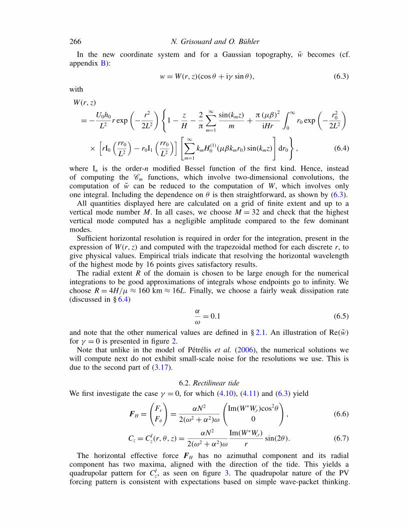
The horizontal effective force FH has no azimuthal component and its radialcomponent has two maxima, aligned with the direction of the tide. This yields aquadrupolar pattern for CI

z, as seen on figure 3. The quadrupolar nature of the PVforcing pattern is consistent with expectations based on simple wave-packet thinking.


1

0

–1

0

0.5

–1

–2

1

–1

0

–0.2 0 0.2

0.5

1

1

2

0

2

–22–2

1.0

0

2

–2

2

1.0

0

(a)

(b)

(c)

FIGURE 2. (Colour online) Re(w)/(aµU0) for γ = 0. Axes are stretched so that waves seemto propagate vertically at angle 45◦. (a,b) horizontal and vertical slices at z = H/2 and θ = 0,respectively (the colour scale applies to both). (c) Three-dimensional isocontours marking theloci where |w|/(aµU0) = 0.1. Blue is for negative values, red for positive, as indicated bythe plus and minus signs. In all three pictures, the double arrow marks the direction of thebarotropic tide. In (a,c), the inner and outer black circles indicate the topographic isocontoursh = h0/2 and h = h0/20, respectively. In (b), the solid line corresponds to the topographyheight multiplied by 4 for purposes of visualization.

For example, as described by e.g. Bretherton (1969) and Buhler (2010), the dissipationof a slowly varying wave packet crossing an isopycnal surface generates a dipolarPV forcing pattern on that isopycnal. In our case, the forcing is now an oscillatingtide, leading to waves that are radiated mainly in two opposite directions and the PVresponse is qualitatively in the form of two dipoles whose PV distributions nearlycancel, i.e. a quadrupole. Another way of seeing the same phenomenon is to note thata quadrupolar PV forcing pattern is a horizontal derivative of a dipolar pattern in FH ,and the spatial integral of such a dipolar FH is zero. This is consistent with a zeromean drag force on the topography over a full tidal oscillation cycle. This is unlike themountain lee-wave scenario, where there is a non-zero drag force on the mountain anda corresponding equal-and-opposite net effective mean force on the fluid, which is feltwhere the waves dissipate. So for lee waves one expects a dipolar PV forcing patternand for tidal waves one expects a quadrupolar pattern.

In this example the numerical magnitude of CIz is ∼2 × 10−6 × aU0ω/L ≈

4 × 10−17 s−2. Using the estimate (5.8) for the time until horizontal advection becomesimportant then yields T ≈ 5 years, which is very long compared to the tidal cycle. IfU0 and h0 were both doubled then by (4.12) the value of Cz would increase by a factorof 16 whilst that of T would decrease by a factor of 4. Still, it seems that one cansafely assume that many tidal cycles will pass before the wave-induced PV disturbancecan no longer be described by our theory.


–1 0 1(× 10–6)

0.5

0

–0.5

0

1.0

0.5

01.0

1.00.50.50

0–0.5–0.5

–1.0 –1.0

1.0

–1.01–1

(a) (b)

FIGURE 3. (Colour online) CIzL/(aU0ω), which corresponds to the same computation as for

figure 2. For explanations of the double arrows, the black lines and the plus and minus signs,see figure 2. (a) A horizontal slice located at altitude z = H/2. Single arrows correspond toFH , their scale being arbitrary. (b) The inner dark and outer light isocontours show the loci of|CI

z|L/(aU0ω) = 2.4 × 10−6 and 0.4 × 10−6, respectively (max[CIzL/(aU0ω)] ≈ 2.7 × 10−6).

6.3. Rotary tide

We now consider γ �= 0, which consists of adding to the previous tide a transversecomponent, in time quadrature with the former. Using again (4.10) and (6.3), we nowhave

FH = αN2

2(ω2 + α2)ω

�Im(W∗W,r)(cos2θ + γ 2sin2θ)

γ |W|2 /r

�. (6.8)

Important qualitative differences arise compared to the γ = 0 case, as the effectiveforce is now the sum of three contributions: in Fr, the contribution of the previous,along-x rectilinear tide proportional to cos2θ and the individual contribution of thetransverse, along-y component proportional to sin2θ ; in Fθ , a cross-term blendingcontributions from both tidal components and responsible for a non-zero azimuthalcomponent of the effective force.

Other consequences of allowing some ellipticity for the rotary barotropic tide aremade apparent in the PV forcing, again with the help of (4.11):

Cz = (1 − γ 2)CIz(r, θ, z) + γ CX

z (r, z), with CXz (r, z) = αN2

(ω2 + α2)ω

Re(W∗W,r)

r. (6.9)

The contributions of each one of the along-x and along-y tidal components, shapedas quadrupoles such as the one displayed in figure 3, are now contained in(1 − γ 2)CI

z. Besides their magnitudes differing by a factor γ 2, the two patterns ofeach individual component are 90o of horizontal rotation from each other around thecentral vertical axis and because they are quadrupolar, they are of opposite sign. Thetwo contributions therefore cancel each other partially for 0 < |γ | < 1 and completelyfor |γ | = 1.

On the other hand, the cross-term γ CXz is independent of θ , as is Fθ . As can be

seen on figure 4, Fθ has its maximum on the slope of the seamount, at a certaindistance from its top and approximately (although not exactly) where CX

z vanishes.


–0.50

0

0

0

0.50.5

(a) (b)

0

1

2

3

4

5

0

0.4

0.6

1.0

0.5 1.00

0.5

1.0

1.5

2.0

0

0.2

0.4

0.6

0.8

1.0

0.5 1.0

0.2

0.8

(× 10–12 m s–2) (× 10–5)

FIGURE 4. Cross-terms forcing the balanced flow in the case where γ �= 0: (a) Fθ/γ and (b)CX

x L/(aU0ω). In (b), the grey scale corresponds to absolute values and contours correspond toalgebraic values, with the −5 × 10−6, 0 and 5 × 10−6 values marked explicitly. The dashedlines in (a) and (b) correspond to the topography height multiplied by 4 for purposes ofvisualization.

0.5

1.0

0.5

0

–1.0 –1.0

–11.0

1.01

–0.5 –0.5

0.50.50

0

00

1.0

0

–1

1

(a) (b)

FIGURE 5. (Colour online) (a) As figure 3(b) but for γ = 0.1. The two outermost isocontourscorrespond to the same values as in figure 3, whereas the innermost isocontour correspondsto CzL/(aU0ω) = 4 × 10−6 (max[CzL/(aU0ω)] ≈ 5.0 × 10−6). The tidal double arrow offigure 3 has turned into a counterclockwise tidal ellipse of aspect ratio γ . (b) As (a) but withviewpoint rotated by 90◦ in the horizontal.

These elements suggest that the cross-terms are forcing a bottom-intensified vortexassociated with (counter-)clockwise displacements around the seamount for γ < 0(γ > 0). We note in passing that computations in Cartesian domains with ellipticinstead of axisymmetric seamounts (not shown) show that the vortex shape actuallyfollows the isobath contours.

To sum up, increasing ellipticity in the rotary barotropic tide decreases themagnitude of the original quadrupolar pattern derived in § 6.2 and increases the forcingof a bottom-intensified vortex, as illustrated in figures 5 and 6 for γ = 0.1 and 0.7.The former shows that even a modest value of γ induces a significant qualitativemodification of Cz near the top of the mountain, while the latter shows how a strong


0.5

1.0

0.5

0

–1.0 –1.0

–11.0

1.01

–0.5 –0.5

0.50.50

0

00

1.0

0

–1

1

(a) (b)

FIGURE 6. (Colour online) As figure 5 but for γ = 0.7, and the innermost isocontour nowcorresponds to CzL/(aU0ω) = 30 × 10−6 (max[CzL/(aU0ω)] ≈ 35 × 10−6).

but realistic (cf. e.g. St Laurent & Garrett 2002) value of γ dramatically changes thePV forcing. The most striking consequence of increasing γ on the PV forcing is theamount that its spatial distribution is modified, becoming more confined to the vicinityof the topography, among other changes. Also, the magnitude of Cz increases sharplywith γ : taking the values computed in § 6.2 for γ = 0 as a reference, its maximumvalue is doubled for γ = 0.1 (cf. figure 5) and multiplied by 14 for γ = 0.7 (cf.figure 6).

6.4. Influence of the dissipation

The value of α that we have used so far, associated with a decay scale of abouta week, is not wildly unreasonable but does not pretend to be realistic and is notdeduced from the literature. Let us now briefly describe how the forcing of the meanflow is modified by variations of α.

Figure 7 shows the γ = 0 and 0.7 cases, for which α/ω = 0.5 (instead of theprevious α/ω = 0.1). The peak values of Cz are now higher than their low-dissipationcounterparts of §§ 6.2 and 6.3, while the low values of Cz occupy roughly the samevolume, corresponding to a more rapid spatial decrease of the mean flow forcing.

Increasing the value of α has the effect of limiting the range of propagation of theO(a) linear waves by increasing their dissipation near the topography. Hence, one canunderstand why the forcing of the mean flow increases in terms of peak value but thatthis increase is limited to the vicinity of the topography. Far from it, the amplitude ofthe wave field is reduced, as is the forcing of the mean flow.

6.5. An example of focusing topography

We have considered so far topography whose isobaths are convex. Buhler & Muller(2007) showed that topographies with concave isobaths could be interesting casesas they could induce three-dimensional focusing of internal waves far from thetopography and hence enhanced wave breaking in those regions.

In order to model a concave topography, we create a horseshoe-shaped topographydefined as

h(r, θ) = h0 exp�

−(r − σ )2

2L2

�cos2

�θ

2

�, (6.10)


0.5

–1 –1

11

00

1.0

0

0.5

–1 –1

11

00

1.0

0

(a) (b)

FIGURE 7. (Colour online) Two cases for which the linear dissipation rate per unit time αis increased from ω/10 to ω/2. (a) As figure 3, with the exception that max[CzL/(aU0ω)] ≈5.9 × 10−6. (b) As figure 6(a), with the exception that max[CzL/(aU0ω)] ≈ 140 × 10−6.

where σ is the distance from the crest of the ridge to the centre of the domain andthe opening along the x < 0 axis is an attempt to model a topographic feature moreplausible than an annulus, resembling a submarine cirque or the mouth of a submarinecanyon. All previous numerical values are kept and we define σ = 3L.

In this configuration, the dependence on θ of w(r, θ, z) is less straightforward thanfor the axisymmetric topography and instead the computations are done on a squareCartesian grid. Owing to the increased computational cost of this procedure, the lateralextent of the semi-domain (equivalent to R in our case) is reduced to 2H/µ and thenumber of computed modes is reduced to M = 16. All other parameters, namely α,the horizontal resolution and all numerical values of the other physical parameters arekept the same. As a result, the computed Cz is somewhat more noisy, which does notdo any harm to the qualitative conclusions we want to draw. More problematic is thepresence of extra artificial noise along the central fluid column, near the bottom. Thisis due to the singularity of the topography gradients in r = 0 and is only significant ifγ �= 0. We therefore set to zero the values of Cz around the origin of the domain in theγ = 0.7 case we study next, which again does not change our qualitative conclusions.

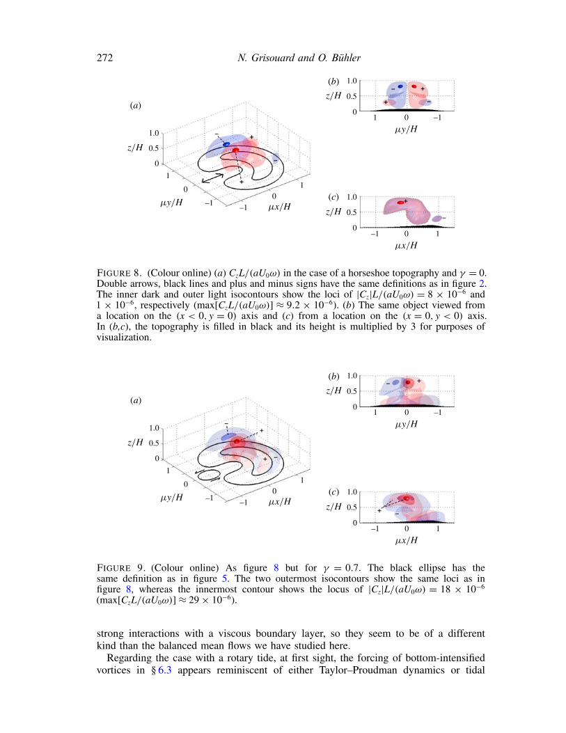
Figures 8 and 9 show that whether γ = 0 or γ = 0.7, Cz peaks around the centre ofthe topography and high above it, where the wave beams converge, therefore agreeingwith the results of Buhler & Muller (2007). Note that for γ = 0, the quadrupolarpattern has virtually disappeared because of the asymmetry of the topography. Suchfocusing topographies could give insights into cases with seamounts with supercriticalslopes, for which wave beams can focus above the summit in a similar way (e.g.Carter, Gregg & Merrifield 2006).

6.6. Comparison with other mean flows around topographies

A clear conceptual distinction exists between our model and other observations, suchas boundary-layer effects or tidal rectification. Unfortunately, they are likely to beconfused with each other in a realistic context, as they seem to produce mean flowswith qualitatively similar features.

To our knowledge, the case presented in § 6.2 of a rectilinear tidal forcing withan axisymmetric mountain has been studied in only a few cases, and only withsupercritical slopes. For example, mean flows at second order in wave amplitude havebeen reported in the laboratory experiments and numerical simulations of King, Zhang& Swinney (2009). However, these mean flows involve significant vertical motion and


0.5

–1 –1

11

00

1.0

0

0.5

1.0

00–1 1

01 –1

0.5

1.0

0(a)

(b)

(c)

FIGURE 8. (Colour online) (a) CzL/(aU0ω) in the case of a horseshoe topography and γ = 0.Double arrows, black lines and plus and minus signs have the same definitions as in figure 2.The inner dark and outer light isocontours show the loci of |Cz|L/(aU0ω) = 8 × 10−6 and1 × 10−6, respectively (max[CzL/(aU0ω)] ≈ 9.2 × 10−6). (b) The same object viewed froma location on the (x < 0, y = 0) axis and (c) from a location on the (x = 0, y < 0) axis.In (b,c), the topography is filled in black and its height is multiplied by 3 for purposes ofvisualization.

0.5

–1 –1

11

00

1.0

0

0.5

1.0

00–1 1

01 –1

0.5

1.0

0(a)

(b)

(c)

FIGURE 9. (Colour online) As figure 8 but for γ = 0.7. The black ellipse has thesame definition as in figure 5. The two outermost isocontours show the same loci as infigure 8, whereas the innermost contour shows the locus of |Cz|L/(aU0ω) = 18 × 10−6

(max[CzL/(aU0ω)] ≈ 29 × 10−6).

strong interactions with a viscous boundary layer, so they seem to be of a differentkind than the balanced mean flows we have studied here.

Regarding the case with a rotary tide, at first sight, the forcing of bottom-intensifiedvortices in § 6.3 appears reminiscent of either Taylor–Proudman dynamics or tidal


rectification (i.e. so-called residual currents). The first class of phenomena can readilybe ruled out as the PV anomaly forcing is not fixed as cyclonic or anticyclonic, but,rather, depends on the sign of γ . Still, the question remains of whether our model isa reinterpretation of tidal rectification or whether it is a phenomenon of a differentnature. We believe the latter is the case, and so we explain in the next paragraphs how‘tidal rectification’ and ‘residual currents’ in the literature describe phenomena that donot include our model.

Tidal rectification has been studied in the shallow-water case by e.g. Huthnance(1973) and Loder (1980) and extended to the stratified case by Maas & Zimmerman(1989a,b). In the shallow-water case, Zimmerman (1981) provides a usefulinterpretation in terms of vorticity dynamics of how residual currents are generated:when flowing above topographies, boundary friction and Coriolis accelerations producetorques on the fluid columns which, integrated over tidal periods, provide a steadyforcing on, say, the circulation around a seamount. In the uniformly stratified case,Maas & Zimmerman (1989a,b) identify the residual current as the zero-frequencyharmonic component, arising when � = O(1) or larger (cf. § 2.2).

Both cases only necessitate studying the interaction of the barotropic tide withitself to generate mean flows. On the contrary, in our case, the barotropic tide andthe mean-flow generation are different by two orders in asymptotic expansion, linearinternal waves providing the link at the intermediate order. For example, if we wereto transpose the mechanism we are describing in the present study to the configurationstudied by Maas & Zimmerman (1989a,b), we would study nonlinear interactionsbetween all wave harmonics. Extending the analogy even further, a similar study ina shallow-water configuration would investigate mean flows generated by dissipativeshallow-water waves generated by the tide–topography system, whereas shallow-watertidal rectification consists of mean flows generated directly and locally by boundaryfriction in the the tide–topography system.

Whether our wave–mean model dominates over tidal rectification is determined bythe excursion parameter �. Assuming � � 1 places us in a case Maas & Zimmerman(1989a) call the ‘deep-sea regime’, for which advection by the barotropic tide andhence the residual currents become negligible, and for which our model dominates theforcing of the mean flow. On the other hand, as first noticed by Zimmerman (1978),problems of tidal rectification involve regimes for which � = O(1), a regime Maas &Zimmerman (1989a) call the ‘continental shelf regime’. As long as the topographicslopes are gentle, our mean-flow forcing will still happen at O(a2), whereas tidalrectification will be an O(1) effect and will therefore dominate.

In regions where tidal excursion is strong, slopes are steep (�, a = O(1)) and meanflows are observed, it could be difficult to determine how much of the aforementionedmean flow is driven by dissipating internal waves or by tidal rectification, because bothmechanisms could be at work (although, strictly speaking, the former would not bedescribed by our weakly nonlinear theory). Unfortunately, our model does not provideany obvious way to solve this puzzle and case-by-case studies would have to be done.In view of these comments, it might be worthwhile to reassess the interpretations ofsome of the observations made in the past in the light of our new model. For example,Kunze & Toole (1997) describe observations of mean flows around Fieberling Guyotwhich could not be related to Taylor–Proudman dynamics, but for which the role oftidal rectification could not be clearly evaluated. Our model might provide a usefulconceptual framework to reinterpret these data.


7. Concluding comments

Our main theoretical result is the derivation of the wave-induced effective force F in(4.10) and of its curl C in (4.11), which we repeat here for convenience:

C = ∇ × F = ∇ × (b�∇ζ ) = αN2

2(ω2 + α2)ω

∇w∗ × ∇wi

. (7.1)

The effective force F differs from b�∇ζ by an irrotational gradient term, which doesnot affect C. Physically, this irrotational gradient term is balanced by a mean pressurefield and therefore does not lead to accelerations of the mean flow.

For a stationary wave field the force curl C comprises the entire effect of thedissipating waves on the mean flow and its vertical component Cz comprises the entireeffect on the Lagrangian-mean PV. The final form in (7.1) depends on the specificwave problem we have investigated, but the form C = ∇ × (b�∇ζ ) holds generallyfor stationary wave fields subject to damping in the buoyancy field. As the verticaldisplacement ζ can be found from ζ,t = w(1) and as b� can be approximated by b(1), itseems that (7.1) could be used for diagnosing numerical simulations or observationaldata for fairly general stationary wave fields subject to buoyancy damping.

Of course, a more complete formulation would allow for dissipative terms in themomentum equation as well. As shown in Buhler (2000), such dissipative termsin the momentum equations add naturally to F provided that these terms aremomentum-conserving in an integral sense (i.e. they derive from the divergenceof a dissipative momentum flux tensor in the usual way). This includes the usualviscous Navier–Stokes terms but excludes Rayleigh damping, for example. Specifically,if a momentum-conserving force D were added to the momentum equations thenone would need to add

�jξj,iD�

j to the ith component of F (e.g. Buhler 2009,§§ 11.1–11.1.1), i.e.

Fi = b�ζ,i +3�

j=1

ξj,iD�j + (. . .),i. (7.2)

This is the most general effective-mean-force formula for the Boussinesq system.Now, one obvious extension of our specific wave problem would be to allow for

finite tidal excursion, which corresponds to allowing the parameter � to take largevalues. As is well known, for the linear dynamics this would produce a polychromaticwave field containing all harmonics of the tidal frequency, with amplitudes generallydecreasing with the order of the harmonic. However, as far as the effective mean forceis concerned, only quadratic combinations with zero frequency matter, which rulesout any correlations between different harmonics. Hence the final term in (7.1) wouldsimply be replaced by a sum over all the harmonics. So, it seems that extending ourtheory to finite excursion length would not lead to fundamentally new results.

To some extent the same could be said if one lifted the restriction to smalltopography amplitude and considered large topography features, simply because (7.1)is a local statement that does not depend on where and how the waves have beengenerated. So, while a three-dimensional numerical wave computation with finite-amplitude topography would certainly be more complicated owing to the possibilityof critical topography slopes as well as the need to apply the boundary conditionsat z = h instead of z = 0, it would seem that the computation of the effective meanforce and its curl would proceed just as in our very simple example. Still, with suchextensions in place it would be interesting to investigate the mean-flow forcing in


realistic settings, such as the aforementioned Fieberling seamount discussed in Kunze& Toole (1997), for example. In such a case, the supercritical topography allows forbeams to propagate upwards and radially inwards. Hence, one might expect to seemean-flow forcing patterns, reminiscent of the patterns described in § 6.5. As discussedin § 6.6 however, competition with tidal rectification would make it not trivial tointerpret the results.

It is interesting to speculate on the long-time behaviour of the mean flow under thePV forcing induced by Cz. After all, the tides are at work relentlessly and there isno shortage of time for effects to accumulate. It seems reasonable to expect that thehorizontal advection terms that have been neglected in (4.14) will eventually lead toself-advection of the PV field away from the forcing region; such behaviour is indeedknown to occur in simpler shallow-water models for vortices generated by breakingwaves on beaches (e.g. Buhler & Jacobson 2001; Barreiro & Buhler 2008). As arguedbefore, in such a scenario the PV will saturate over a time scale proportional to 1/

√Cz

and at an amplitude scaling with√

Cz, which from (7.1) and the definition of thewave slope µ would indicate that the PV amplitude scales as

�α(ω2 − f 2)/ω times

the root-mean-square value of ζ,z. The latter is the non-dimensional amplitude of thewaves and can therefore be expected to be of order unity for breaking waves. Henceone can estimate that the saturated PV amplitude should scale as

�α(ω2 − f 2)/ω.

Finally, it would be very interesting to see via numerical simulation of the fullynonlinear system whether these saturation estimates for the PV are viable or not.However, as noted before, such simulations would have to be three-dimensional inorder to capture this kind of secularly growing PV dynamics, which is entirely absentin two-dimensional models, and a configuration keeping a and � small would have tobe integrated for years before reaching saturation. At present, this perhaps makes suchsimulations prohibitively expensive.

Acknowledgements

Fruitful discussions with R. Ferrari, J. McWilliams, E. D’Asaro and especiallyL. Maas are acknowledged. The authors also thank three anonymous refereesfor helping us improve the article. Financial support under the USA NationalScience Foundation grants NSF/OCE 1024180 and NSF/DMS 1009213 is gratefullyacknowledged.

Appendix A. Linear vertical velocity in two dimensions

We are looking for a solution of (3.5) in two dimensions (∂/∂y = 0), using the sameapproach as in § 3.2. We are now solving for G(x, z; x0):

G,xx − (µβ)2 G,zz = 0 for (x, z) �= (x0, 0), (A 1a)G|z=H = 0; G|z=0 = δ(x − x0), (A 1b)

and proceed to the same decomposition of G that lead to (3.9):

G(x, z; x0) = G (x, z; x0) +�

1 − zH

�δ(x − x0). (A 2)

We then reproduce the series of operations spanning from (3.10) to (3.12) for whichwe now have to solve for each Gm an inhomogeneous one-dimensional Helmholtz


equation of wavenumber µβkm, whose Green’s function is

gm(x; x1) = exp(iµβkm|x − x1|)2iµβkm

. (A 3)

Integrating over R instead of R2, we get the the equivalent of (3.15):

Gm(x; x0) = − 2πm

gm,xx(x; x0) = µβ

iHexp(iµβkm|x − x0|) − 2

πmδ(x − x0), (A 4)

the final expression for Gm having been obtained using the one-dimensional Helmholtzequation that gm is a Green’s function of. The final expression for G is therefore

G(x, z; x0) = µβ

iH

∞�

m=1

exp(iµβkm|x − x0|) sin(kmz)

+�

1 − zH

− 2π

∞�

m=1

sin(kmz)m

�δ(x − x0), (A 5)

which yields (3.19) and (3.20).

Appendix B. Linear vertical velocity expressed in polar coordinates

Let us recall the expression for w0 in Cartesian coordinates:

w0(x, y) = −U0h0

L2(x + iγ y) exp

�−x2 + y2

2L2

�, (B 1)

and hence, in polar coordinates:

w0(r − r0) = −U0h0

L2[r cos θ − r0 cos θ0 + iγ (r sin θ − r0 sin θ0)]

× exp�

−r2 + r20 − 2rr0 cos(θ − θ0)

2L2

�. (B 2)

Equation (3.18) consists of a convolution. After inverting r0 and |r − r0| in it, wefind

Cm(r, θ) = −U0h0km

L2exp

�− r2

2L2

� � ∞

0r0H(1)

0 (µβkmr0)

× exp�

− r20

2L2

�ψ(r, r0, θ) dr0, (B 3)

where

ψ(r, r0, θ) =� 2π

0[r cos θ − r0 cos θ0 + iγ (r sin θ − r0 sin θ0)]

× exp�

rr0 cos(θ − θ0)

L2

�dθ0. (B 4)

Performing the variable change Θ = θ − θ0, dΘ = −dθ0 and expanding thetrigonometric functions yields

ψ(r, r0, θ) = 2π(cos θ + iγ sin θ)�rI0

�rr0

L2

�− r0I1

�rr0

L2

��. (B 5)


In the equation above, In is the order-n modified Bessel function of the first kind,which for (n, x) ∈ (Z, C) can be defined as (cf. Olver et al. 2010, § 10.32)

In(x) = 1π

� π

0cos(nΘ)ex cos Θ dΘ. (B 6)

Equation (B 3) hence becomes

Cm = 2πkmw0(r, θ)

r

� ∞

0r0H(1)

0 (µβkmr0)

× exp�

− r20

2L2

� �rI0

�rr0

L2

�− r0I1

�rr0

L2

��dr0, (B 7)

which yields (6.3).

R E F E R E N C E S

ANDREWS, D. G., HOLTON, J. R. & LEOVY, C. B. 1987 Middle Atmosphere Dynamics, 1st edn.Academic.

ANDREWS, D. G. & MCINTYRE, M. E. 1978 An exact theory of nonlinear waves on aLagrangian-mean flow. J. Fluid Mech. 89 (4), 606–646.

BARREIRO, A. K. & BUHLER, O. 2008 Longshore current dislocation on barred beaches.J. Geophys. Res. 113, C12004.

BARTON, G. 1989 Elements of Green’s Functions and Propagation: Potentials, Diffusion, and Waves.Oxford University Press.

BELL, T. H. 1975 Lee waves in stratified flows with simple harmonic time dependence. J. FluidMech. 67 (4), 705–722.

BRETHERTON, F. P. 1969 On the mean motion induced by internal gravity waves. J. Fluid Mech. 36(4), 785–803.

BUHLER, O. 2000 On the vorticity transport due to dissipating or breaking waves in shallow-waterflow. J. Fluid Mech. 407, 235–263.

BUHLER, O. 2009 Waves and Mean Flows. Cambridge University Press.BUHLER, O. 2010 Wave–vortex interactions in fluids and superfluids. Annu. Rev. Fluid Mech. 42,

205–228.BUHLER, O. & JACOBSON, T. E. 2001 Wave-driven currents and vortex dynamics on barred beaches.

J. Fluid Mech. 449, 313–339.BUHLER, O. & MCINTYRE, M. E. 1998 On non-dissipative wave-mean interactions in the

atmosphere or oceans. J. Fluid Mech. 354, 301–343.BUHLER, O. & MCINTYRE, M. E. 2003 Remote recoil: a new wave–mean interaction effect.

J. Fluid Mech. 492, 207–230.BUHLER, O. & MULLER, C. J. 2007 Instability and focusing of internal tides in the deep ocean.

J. Fluid Mech. 588, 1–28.CARTER, G. S., GREGG, M. C. & MERRIFIELD, M. A. 2006 Flow and mixing around a small

seamount on Kaena Ridge, Hawaii. J. Phys. Oceanogr. 36 (6), 1036–1052.ECHEVERRI, P. & PEACOCK, T. 2010 Internal tide generation by arbitrary two-dimensional

topography. J. Fluid Mech. 659, 247–266.GARRETT, C. & KUNZE, E. 2007 Internal tide generation in the deep ocean. Annu. Rev. Fluid Mech.

39, 57–87.HUTHNANCE, J. 1973 Tidal current asymmetries over the Norfolk Sandbanks. Estuar. Coast. Mar.

Sci. 1 (1), 89–99.KING, B., ZHANG, H. P. & SWINNEY, H. L. 2009 Tidal flow over three-dimensional topography in

a stratified fluid. Phys. Fluids 21 (11), 116601.KUNZE, E. & TOOLE, J. M. 1997 Tidally driven vorticity, diurnal shear, and turbulence atop

fieberling seamount. J. Phys. Oceanogr. 27 (12), 2663–2693.


LEDWELL, J. R., MONTGOMERY, E. T., POLZIN, K. L., ST. LAURENT, L. C., SCHMITT, R. W. &TOOLE, J. M. 2000 Evidence for enhanced mixing over rough topography in the abyssalocean. Nature 403 (6766), 179–182.

LLEWELLYN SMITH, S. G. & YOUNG, W. R. 2002 Conversion of the barotropic tide. J. Phys.Oceanogr. 32 (5), 1554–1566.

LLEWELLYN SMITH, S. G. & YOUNG, W. R. 2003 Tidal conversion at a very steep ridge. J. FluidMech. 495, 175–191.

LODER, J. W. 1980 Topographic rectification of tidal currents on the sides of Georges bank. J. Phys.Oceanogr. 10 (9), 1399–1416.

MAAS, L. R. M. & ZIMMERMAN, J. T. F. 1989a Tide-topography interactions in a stratified shelfsea I. Basic equations for quasi-nonlinear internal tides. Geophys. Astrophys. Fluid Dyn. 45(1–2), 1–35.

MAAS, L. R. M. & ZIMMERMAN, J. T. F. 1989b Tide-topography interactions in a stratified shelfsea II. Bottom trapped internal tides and baroclinic residual currents. Geophys. Astrophys.Fluid Dyn. 45 (1–2), 37–69.

MCINTYRE, M. E. & NORTON, W. A. 1990 Dissipative wave-mean interactions and the transport ofvorticity or potential vorticity. J. Fluid Mech. 212, 403–435.

MULLER, C. J. & BUHLER, O. 2009 Saturation of the internal tides and induced mixing in theabyssal ocean. J. Phys. Oceanogr. 39 (9), 2077–2096.

NIKURASHIN, M. & FERRARI, R. 2010a Radiation and dissipation of internal waves generated bygeostrophic motions impinging on small-scale topography: application to the southern ocean.J. Phys. Oceanogr. 40 (9), 2025–2042.

NIKURASHIN, M. & FERRARI, R. 2010b Radiation and dissipation of internal waves generated bygeostrophic motions impinging on small-scale topography: theory. J. Phys. Oceanogr. 40 (5),1055–1074.

OLVER, F. W. J., LOZIER, D. W., BOISVERT, R. F. & CLARK, C. W. (Eds) 2010 NIST Handbookof Mathematical Functions. Cambridge University Press.

PETRELIS, F., LLEWELLYN SMITH, S. & YOUNG, W. R. 2006 Tidal conversion at a submarineridge. J. Phys. Oceanogr. 36 (6), 1053–1071.

POLZIN, K. L., TOOLE, J. M., LEDWELL, J. R. & SCHMITT, R. W. 1997 Spatial variability ofturbulent mixing in the abyssal ocean. Science 276 (5309), 93–96.

ROBINSON, R. M. 1969 The effects of a vertical barrier on internal waves. Deep Sea Res. Oceanogr.Abstracts 16 (5), 421–429.

ST LAURENT, L. & GARRETT, C. 2002 The role of internal tides in mixing the deep ocean. J. Phys.Oceanogr. 32 (10), 2882–2899.

ZEILON, N. 1912 On tidal boundary-waves and related hydrodynamical problems. Kungl. SvenskaVetenskapsakademiens Handlingar 47 (4), 3–45.

ZIMMERMAN, J. T. F. 1978 Topographic generation of residual circulation by oscillatory (tidal)currents. Geophys. Astrophys. Fluid Dyn. 11 (1), 35–47.

ZIMMERMAN, J. T. F. 1981 Dynamics, diffusion and geomorphological significance of tidal residualeddies. Nature 290 (5807), 549–555.

Date post:	03-Apr-2022
Category:	Documents
Upload:	others
View:	4 times
Download:	0 times

J. Fluid Mech. (2012), . 708, pp. 250–278. doi:10.1017/jfm ...

Documents