J. Fluid Mech. (2015), . 772, pp. doi:10.1017/jfm.2015.186 ...

J. Fluid Mech. (2015), vol. 772, pp. 42–79. c© Cambridge University Press 2015doi:10.1017/jfm.2015.186

42

The effect of shear flow on the rotationaldiffusion of a single axisymmetric particle

Brian D. Leahy1,†, Donald L. Koch2 and Itai Cohen1

1Department of Physics, Cornell University, Ithaca, NY 14853, USA2Department of Chemical Engineering and Biomolecular Engineering, Cornell University, Ithaca,

NY 14853, USA

(Received 2 October 2014; revised 30 January 2015; accepted 20 March 2015;first published online 28 April 2015)

Understanding the orientation dynamics of anisotropic colloidal particles is importantfor suspension rheology and particle self-assembly. However, even for the simplestcase of dilute suspensions in shear flow, the orientation dynamics of non-sphericalBrownian particles are poorly understood. Here we analytically calculate the time-dependent orientation distributions for non-spherical axisymmetric particles confinedto rotate in the flow–gradient plane, in the limit of small but non-zero Browniandiffusivity. For continuous shear, despite the complicated dynamics arising from theparticle rotations, we find a coordinate change that maps the orientation dynamics to adiffusion equation with a remarkably simple ratio of the enhanced rotary diffusivity tothe zero shear diffusion: Dr

eff /Dr0= (3/8)(p− 1/p)2+ 1, where p is the particle aspect

ratio. For oscillatory shear, the enhanced diffusion becomes orientation dependent anddrastically alters the long-time orientation distributions. We describe a general methodfor solving the time-dependent oscillatory shear distributions and finding the effectivediffusion constant. As an illustration, we use this method to solve for the diffusion anddistributions in the case of triangle-wave oscillatory shear and find that they dependstrongly on the strain amplitude and particle aspect ratio. These results provide newinsight into the time-dependent rheology of suspensions of anisotropic particles. Forcontinuous shear, we find two distinct diffusive time scales in the rheology that scaleseparately with aspect ratio p, as 1/Dr

0p4 and as 1/Dr0p2 for p 1. For oscillatory

shear flows, the intrinsic viscosity oscillates with the strain amplitude. Finally, weshow the relevance of our results to real suspensions in which particles can rotatefreely. Collectively, the interplay between shear-induced rotations and diffusion hasrich structure and strong effects: for a particle with aspect ratio 10, the oscillatoryshear intrinsic viscosity varies by a factor of ≈2 and the rotational diffusion by afactor of ≈40.

Key words: colloids, rheology, suspensions

1. IntroductionStir a solution and the solute will mix faster than when the solution is left quiescent.

This mixing is enhanced even at low Reynolds numbers due to the coupling of random

† Email address for correspondence: [email protected]

mailto:[email protected]

The effect of shear flow on the rotational diffusion of a particle 43

Brownian motion and spatially-varying fluid velocities. Brownian motion causes soluteparticles to access different fluid streamlines, which in turn differentially advect thesolute particles. On long times, this combination of diffusion and advection looksthe same as an enhanced translational diffusion. This mechanism, known as Taylordispersion, occurs in a wide variety of natural and industrial processes ranging fromdrug delivery in the bloodstream (Fallon, Howell & Chauhan 2009) to microfluidiclab-on-a-chip setups (Datta & Ghosal 2009), with high Reynolds number analogueseven determining mixing in streams and rivers (Fischer 1973). Taylor dispersion isonly one example of the broader coupling that occurs between advection and diffusionthat is used to manipulate mass transport across many scales, ranging from chaoticmixing in microchannels (Stroock et al. 2002) to particle clustering in turbulent fluids(Balkovsky, Falkovich & Fouxon 2001).

Anisotropic particles allow for more complex coupling between diffusion andconvection, due to the additional orientational degrees of freedom they possess.Under shear, an isolated ellipsoid’s orientation is not constant, but instead rotateswith the flow in an unsteady motion known as a Jeffery orbit (Jeffery 1922).In colloidal suspensions, rotational Brownian motion also changes the particles’orientations, creating the possibility of a coupling between the Jeffery orbit androtational diffusion. Recently, through experiments and simulations Leahy et al.(2013) observed an enhancement of the rotational diffusion for colloidal dimers undershear, suggesting that such a coupling does exist. However, little is known about thiscoupling compared to its translational counterparts.

In this paper, we take the first steps towards calculating analytically the effectsof rotary diffusion coupled with Jeffery orbits. In the rest of § 1, we first reviewprevious work on the effects of rotational diffusion coupled with Jeffery orbits. In§ 2, we find the time-dependent orientation distribution for a dilute suspension ofaxisymmetric particles subjected to continuous shear. To make the analysis tractable,we examine the limit where the shear rate is large (i.e. Pe 1, where the Pécletnumber Pe ≡ γ /Dr

0 is the ratio of the shear rate to the zero-shear rotary diffusionconstant), and we restrict the particle orientations to reside in the flow–gradient plane,which is a representative Jeffery orbit. Remarkably, we find that the complicatedconvection–diffusion equation describing the particle’s orientations maps to a simplediffusion equation in a new coordinate with an enhanced diffusion constant. In § 3,we generalize these results to derive the time-dependent evolution of non-sphericalparticle orientations under oscillatory shear. Even in the limit of large shear rates,the oscillatory shear distributions and diffusive dynamics differ considerably fromthe continuous shear distributions. In § 4, we examine particular solutions of theoscillatory shear equations, taking triangle-wave shear as an analytically tractableexample. In § 5, we use our results to explore how rotational diffusion affects therheology of a suspension of non-spherical particles at large shear rates. Finally, in § 6,we close by comparing our results to traditional Taylor dispersion and demonstratingtheir relevance to real three-dimensional particle orientations.

While Jeffery explained the rotation of an ellipsoid, his solution does not addressparticles of other shapes. However, symmetry and group theory arguments can beused to ascertain how a general particle rotates (Happel & Brenner 1983). For anaxisymmetric particle, the orientation is completely specified by a unit normal n. Asshown by Bretherton (1962), any axisymmetric particle in Stokes flow rotates in aJeffery orbit as:

dndt= n ·Ω + λ[E · n− n (n · E · n)]. (1.1)

44 B. D. Leahy, D. L. Koch and I. Cohen

Here Ω and E are the fluid vorticity and rate-of-strain tensors, Ωij ≡ (∂iuj − ∂jui)/2and E ij ≡ (∂iuj + ∂jui)/2. The coefficient λ is a scalar constant which depends on theparticle geometry and can be found from solving the full Stokes equations. Jeffery(1922) showed for an ellipsoid of revolution that λ≡ (p2− 1)/(p2+ 1), where p is theparticle aspect ratio. For simple, continuous shear with strain rate γ , (1.1) simplifiesconsiderably. If |λ|< 1, which is usually the case, then the magnitude of the secondterm is always less than the first term, and the particle rotates indefinitely. Denoting θas the polar angle measured from the vorticity direction and φ as the azimuthal anglefrom the gradient direction in the flow–gradient plane, (1.1) admits the solution

tan φ = p tan(

γ tp+ 1/p

+ κ),

tan θ =C(

p cos2 φ + 1p

sin2 φ

)−1/2

,

(1.2)

where p is an effective aspect ratio and the phase angle κ and orbit constant C capturethe particle’s initial orientation. Equations (1.1) and (1.2) show a symmetry underthe transformation p→ 1/p, φ→ φ + π/2; thus, the motion of disc-like and rod-likeparticles is the same up to a change of axes. Note that (1.2) employs a differentdefinition of C than usual in the literature to emphasize the p → 1/p symmetry.The particle rotates in one of an infinite number of Jeffery orbits, each of whichis described by an orbit constant C determined by the particle’s initial orientation.Since the orbits are periodic, there is no mechanism to select a unique long-timedistribution of orientations.

In colloids, rotational diffusion also affects the particles’ orientations. Theprobability distribution ρ of finding a rod at orientation (θ, φ) is given by aFokker–Planck equation:

∂ρ

∂t=Dr

0∇2ρ −∇ · (ρu), (1.3)

u= φγ

p+ 1/p

(p cos2 φ + 1

psin2 φ

)sin θ + θ

γ (p2 − 1)4(p2 + 1)

sin 2φ sin 2θ. (1.4)

Here t is the time, Dr0 is the rotary diffusion constant, u is the Jeffery orbit’s rotary

velocity field from (1.1), φ and θ are unit vectors in the φ and θ directions, andthe divergence and Laplacian operators act in orientation space (θ, φ). The relativestrength of the diffusive term Dr

0∇2ρ to the advective term ∇ · (ρu) is quantifiedby a rotary Péclet number Pe = γ /Dr

0. While ordinarily the diffusion in (1.3) isdue to Brownian motion, (1.3) has also been used to capture the effects of randomhydrodynamic interactions in non-Brownian fibre suspensions at finite concentrations(Folgar & Tucker 1984; Rahnama, Koch & Shaqfeh 1995). As a result, (1.3) hasbeen analysed in many different limiting values of the Péclet number, which we nowdescribe.

Low shear rates, Pe 1. When there is no shear, (1.3) reduces to a simple diffusionequation, and the particle orientations become isotropically distributed on timeslonger than 1/Dr

0. When Pe is small but non-zero, the distribution can be foundthrough a straightforward perturbation approach. If the particle is elongated (p > 1),to first order in Pe the steady-state orientation distribution is enhanced along theflow’s extensional axis, where the Jeffery orbit has a negative divergence, and the


distribution is suppressed along the flow’s compressive axis, where the Jeffery orbithas a positive divergence. This perturbation expansion can be extended to yield apower series in Pe = γ /Dr

0 (Peterlin 1938; Stasiak & Cohen 1987; Strand, Kim &Karrila 1987) and has been evaluated numerically up to many orders in Pe. However,the series does not converge for Pe & 1, and other methods must be used to find thedistribution for such flows (Kim & Fan 1984).

High shear rates, Pe 1. Early attempts to calculate the distributions in the limit ofweak diffusion simply looked for a steady-state solution to (1.3) with Dr

0=0. However,this procedure produces an apparent indeterminacy in ρ, since without diffusion thereis no mechanism to select a steady-state distribution of orbit constants. Leal and Hinchrealized that weak diffusion primarily acts to select a distribution of the particles’phase angles κ and orbit constants C (Leal & Hinch 1971; Hinch & Leal 1972).When p 1 the mode of the steady-state distribution has an orbit constant C ≈√

p/8, corresponding to an orbit that bends strongly towards the flow direction whenφ = π/2 but returns to a moderate distance away from the gradient direction whenφ= 0. Diffusion also randomizes κ and orients most particles near the flow direction,where the orbit’s rotational velocity is slow. As a result, the steady-state distributionis strongly aligned with the flow for large p.

Intermediate shear rates, 1 Pe (p + 1/p)3. When the particle aspect ratio islarge p 1, (1.4) shows that the particle rotates extremely slowly when orientednear the flow direction. As a result, for large p it is possible for the Jeffery orbitto be dominant compared to diffusion over most of the orbit, but for diffusion tobe important in a small orientational boundary layer of size ∼1/p near φ = π/2.Hinch & Leal (1972) showed that in this intermediate regime (1 Pe p3), thefraction of particles oriented away from the flow direction decreases as ∼1/Pe1/3.These predictions at high and intermediate Pe have been verified experimentally, bothquantitatively (Vadas et al. 1976) and qualitatively (Frattini & Fuller 1986; Gason,Boger & Dunstan 1999; Jogun & Zukoski 1999; Brown et al. 2000; Pujari et al.2009; Leahy et al. 2013).

Dynamics. The time evolution of ρ is of interest since it determines the startuprheology of a suspension of rod-like particles. At low Pe, the time dynamics aredetermined by rotational diffusion, and there is only one time scale of interest. AtPe = 0, the evolution of the particle orientations is described by a simple diffusionequation, which has been studied extensively (Furry 1957; Hubbard 1972; Valiev& Ivanov 1973). At low but non-zero Pe, the dynamics of (1.3) have been studiedsince Peterlin (1938) through series expansions in Pe, partly as a model of polymericsolutions under startup flows. At second order and higher in Pe, the orientationtransients in a suspension cause a stress overshoot, followed by an undershoot (Bird,Warner & Evans 1971; Stasiak & Cohen 1987; Strand et al. 1987).

At high Pe the time variation due to the Jeffery orbit becomes important. However,since the rotation is periodic, the Jeffery orbit by itself does not lead to a steady-statedistribution. The distribution in (1.3) instead approaches steady state due to diffusion,which occurs on a longer time scale. Thus, in contrast to the low Pe case, at high Pethere are two time scales which determine the evolution of ρ. The time-dependence ofρ due to the Jeffery orbit at high Pe has been well-studied. At short times, the Jefferyorbit causes oscillations in ρ, which have been observed experimentally through directimaging (Okagawa, Cox & Mason 1973; Okagawa & Mason 1973), flow dichroism(Frattini & Fuller 1986; Krishna Reddy et al. 2011), and suspension rheology (Ivanov,van de Ven & Mason 1982).


Comparatively less work has focused on the approach of ρ to steady state dueto diffusion. Hinch & Leal (1973) attempted to solve (1.3) exactly by separation ofvariables. While they were not able to obtain an exact solution, they made scalingarguments based on the orthogonality of the eigenfunctions of the convection–diffusionoperator to qualitatively understand the time evolution of ρ, arguing that at high Pethere were two diffusive time scales in the rheology. Recently, through a combinationof experiments and simulation Leahy et al. (2013) showed that oscillatory shear athigh Pe enhances rotational diffusion, as measured from the orientational correlations.This enhancement was attributed to a mechanism where rotational diffusion allowsdifferent particles to access regions of different rotational velocity, leading to anenhanced effective diffusion. An analytical solution of the rotational dynamics undershear would provide additional insight into the effect of shear on rotational diffusion.

2. Orientation dynamics under continuous shearA full time-dependent solution to (1.3) has not been found for over seventy years.

Even in the limit of large shear rates (Pe 1), a uniformly valid time-dependentsolution does not exist. Rather than attempt to solve (1.3) exactly, then, we examinethe case where the particle is restricted to the most extreme Jeffery orbit along theflow–gradient plane (i.e. θ =π/2). Equation (1.3) then simplifies to

∂ρ

∂t=Dr

0∂2ρ

∂φ2− ∂

∂φ[ρu(φ)],

u(φ)= γ

p+ 1/p

(p cos2 φ + 1

psin2 φ

).

(2.1)

Since this Jeffery orbit has the largest variation in angular velocities and isrepresentative of the Jeffery orbit’s φ dynamics, we expect that it captures theessence of the orientation dynamics along the Jeffery orbits in three dimensions; wedefer a discussion of three-dimensional orientation dynamics to § 6.

At high Pe, the complicated advective term is dominant, while the much simplerdiffusive term is weak. The reverse case would be easier to treat: if the advective termwere simple and the diffusion term complicated, we could hope to solve the dominantadvective portion exactly and to treat the weak diffusion with a singular perturbationscheme. When written in the φ-coordinate, the advective term is complicated dueto the rotation of the Jeffery orbit. This suggests that we parameterize the particle’sorientation by a coordinate that does not change due to the Jeffery orbit. We definenew coordinates (κ, t′) such that

∂κ

∂φ= u

u(φ),∂κ

∂t=−u,

∂t′

∂φ= 0,

∂t′

∂t= 1,

(2.2)

where u is the mean velocity over an entire Jeffery orbit, i.e. u≡1φ/TJO = γ /(p+1/p) where 1φ = 2π and TJO is the Jeffery orbit period from (1.2). The constant unon-dimensionalizes the velocity; the reason for this choice is discussed in § 3. For aJeffery orbit, the new coordinates are the same as the phase angle defined in (1.2):

p tan(ut′ + κ)≡ tan φ, (2.3)t′ ≡ t; (2.4)


(a) (b) (c)

FIGURE 1. (Colour online) The continuous-shear distributions ρ(φ) from (2.14) for aparticle with aspect ratio p≈ 2.83. (a) ρ(φ) in steady state. Here the value of ρ is shownby the distance from the central black ring; the dotted black line shows the zero-shearequilibrium distribution (ρ= 1/2π). The solid black lines correspond to 12 equally-spacedangles at φ = nπ/6. The red arrows indicate the Jeffery orbit velocity (1.1). (b,c) Theancillary distribution f in the stretched space. The angular portion of (2.3), shown in (b),stretches the space significantly, visible from the bunched φ gridlines, and turns the Jefferyorbit into a uniform rotation. By transforming to a rotating reference frame (c), theuniform rotation in (b) is removed.

the definition in (2.2) gives a construction of κ for arbitrary rotary velocity fields.These coordinates are illustrated schematically in figure 1. Under the angular portionof the coordinate change, lines spaced by constant φ (figure 1a) get bunched in κ(figure 1b) to reflect the velocity differences along the orbit, causing the particles’motion (red arrows) to look like a uniform rotation. This angular portion of thecoordinate change is the coordinate space used by Leal & Hinch (1971) to determinethe steady-state distributions under continuous shear. The t dependence of κ in (2.2)removes this uniform rotation (figure 1c).

In this new phase-angle coordinate κ , advection due to the Jeffery orbit iscompletely removed. The probability of finding a particle with a phase angle in(κ, κ + dκ) evolves solely due to diffusion. Thus, instead of writing (2.1) withthe distribution ρ(φ), we recast (2.1) in terms of an ancillary distribution f (κ) thatdescribes the probability of finding a particle in the region (κ, κ + dκ):

f (κ)≡ ρ ∂φ∂κ= ρ u

u. (2.5)

With the new coordinates (κ, t′) and the ancillary distribution f , (2.1) can be recastinto a simpler form. Direct substitution of the definition of f into (2.1) gives

uu(φ)

∂f∂t=Dr

0∂2

∂φ2

(u

u(φ)f)− u

∂f∂φ. (2.6)

Transforming the derivatives to the new coordinates, (2.6) can be written after somesimple rearrangements as

∂f∂t′=Dr

0∂

∂κ

[uu∂

∂κ

(uu

f)]

, where

uu(φ)=[

p cos2 φ + 1p

sin2 φ

]−1

= 1p

cos2(κ + ut)+ p sin2(κ + ut).

(2.7)


This construction of κ and f (κ) results in an ancillary distribution f that does notmove with the Jeffery orbit; all the time evolution of f (κ) arises from diffusion,as visible from (2.7). The initial equation (2.1) is a complicated partial differentialequation in simple coordinates. By making the coordinate change φ→ κ , (2.1) hasbeen transformed into a more tractable partial differential equation in complicatedcoordinates. Since the coordinate change is straightforward, we can analyse (2.7) inthe stretched coordinates to understand the rod’s dynamics, and easily transform backto φ afterward.

Equation (2.7) is exact, describing both the significant long-time diffusion of theparticle orientations and the small, less important short-time changes due to couplingbetween the Jeffery orbits and diffusion. To understand the orientation distributionwhen diffusion is small, we introduce a dimensionless advective time t= ut′ and thedimensionless diffusion or inverse Péclet number ε ≡ Dr

0/u. In dimensionless form,(2.7) then becomes

∂f∂t= ε ∂

∂κ

[uu∂

∂κ

(uu

f)]

. (2.8)

We wish to understand the evolution of f on long times t& 1/ε, in the limit ε→ 0.To isolate the long-time behaviour, we find the net change of f after a full Jefferyorbit by integrating (2.7) over a period of a Jeffery orbit, uTJO = 2π. Expanding thederivatives in (2.8) and integrating gives

f (κ, t+ 2π) = f (κ, t)+ ε∫ t+2π

t

(u

u(φ(κ, τ ))

)2∂2f∂κ2

dτ

+ 32

∫ t+2π

t

∂

∂κ

(u

u(φ(κ, τ ))

)2∂f∂κ

dτ

+ 12

∫ t+2π

t

∂2

∂κ2

(u

u(φ(κ, τ ))

)2

f dτ

, (2.9)

where τ is a dummy variable of the integration.By assuming that the diffusion is weak (i.e. the dimensionless diffusion ε≡Dr

0/u1), these integrals can be simplified considerably. Since f changes slowly with time,cf. (2.8), f and its derivatives in κ can be Taylor expanded in t about t= 0 : f (κ, t)=f (κ, 0)+ t∂f /∂t(t = 0)+ O(t2). But by construction ∂f /∂t= O(ε), so f (κ, t) can beapproximated by f (κ, 0), with a correction to (2.9) of O(ε2). In contrast, the functionu(κ + t) cannot be approximated by u(κ), since ∂u/∂t is O(1). Thus, to first order inε, (2.9) can be written as

f (κ, t+ 2π)− f (κ, τ ) = ε

∂2f∂κ2

∫ t+2π

t

(u

u(κ + τ))2

dτ

+ 32∂f∂κ

∫ t+2π

t

∂

∂κ

(u

u(κ + τ))2

dτ

+ 12

f∂2

∂κ2

∫ t+2π

t

(u

u(κ + τ))2

dτ

+O(ε2). (2.10)

This finite-time update equation can be recast as a differential equation in the limitε→ 0. Define a new dimensionless time τ ≡ εt≡Dr

0t. Rewriting the integrals in (2.10)


as averages gives

f (κ, τ + 2πε)− f (κ, τ )2πε

=⟨(

uu

)2⟩∂2f∂κ2+ 3

2∂

∂κ

⟨(uu

)2⟩∂f∂κ+ 1

2∂2

∂κ2

⟨(uu

)2⟩

f

(2.11)

where 〈·〉 denotes the average over a Jeffery orbit period. In the limit of large shearrates ε → 0, and this update equation becomes a differential equation. Re-castingback to the dimensional (κ, t′) coordinates, (2.10) can be written as the differentialequation

∂f∂t′=Dr

0

[⟨(uu

)2⟩∂2f∂κ2+ 3

2

⟨∂

∂κ

(uu

)2⟩∂f∂κ+ 1

2

⟨∂2

∂κ2

(uu

)2⟩

f +O(ε)

].

(2.12)

In addition, the second and third integrals on the right-hand side of (2.12) canbe simplified. Since the rotation rate u is a function of κ + ut′ only, cf. (2.7), thederivatives of u can be rewritten as ∂u/∂κ = u∂u/∂t′. Consequently, the second andthird terms become integrals of a derivative, and vanish since u and its derivative areperiodic. As a result, only the first of the three integrals in (2.12) is non-zero.

Remarkably, in the limit ε → 0 these manipulations transform the complexorientation dynamics in (2.1) into a simple diffusion equation with a uniform diffusionconstant:

∂f∂t′=Dr

0

⟨(uu

)2⟩∂2f∂κ2

, (2.13)

where the angle brackets denote a time-average over one orbit. On long times, therod’s orientation moves diffusively in the stretched space with an effective diffusionconstant Dr

eff = Dr0〈(u/u)2〉. When diffusion is small, it acts to randomize the phase

angle κ of the rod’s Jeffery orbit. While the randomizing kicks of diffusion coupledto the Jeffery orbit do not produce diffusive behaviour in real φ-space, their combinedeffect results in an emergent simple diffusion in the stretched κ-space.

Up to this point, none of the results depend on the specific form of the Jeffery orbit.All that is required to proceed up to (2.13) is a rotary velocity field u(φ) that is non-zero and gives rise to periodic orbits, allowing for an appropriate coordinate change.The details of the Jeffery orbit only enter into the value of the effective diffusionconstant Dr

eff and in the definition of κ and f (κ). At long times, f (κ)= 1/2π and κis completely randomized, giving a steady-state distribution

ρ(φ)= 12π[p cos2 φ + 1/p sin2 φ]−1, (2.14)

i.e. rods with p > 1 mostly orient along the flow direction (φ ≈ π/2), where theJeffery orbit velocity is slowest, cf. figure 1. This long-time distribution is the two-dimensional version of Leal and Hinch’s solution.

More importantly, our derivation also allows us to calculate an analytical solutionfor the orientation dynamics. Evaluating the average 〈(u/u)2〉 we find a simple formfor the effective diffusion constant Dr

eff :

Dreff /D

r0 = 3

8(p− 1/p)2 + 1. (2.15)


Equation (2.15) states that the effective diffusion of rod-like particles is enhancedunder shear, in agreement with experiments in three dimensions (Leahy et al. 2013).The effective diffusion constant Dr

eff is symmetric with respect to p→ 1/p, respectingthe symmetry of the Jeffery orbits. For spherical particles, which have p = 1 andundergo uniform rotation, the rotational diffusion is not enhanced: Dr

eff (p= 1)/Dr0= 1.

Just as Taylor dispersion requires non-uniform translational velocities to enhance thediffusion, a non-uniform Jeffery orbit is required to enhance the rotational diffusion.

The ∼p2 enhancement of the diffusion for p 1 can be understood from thestructure of the Jeffery orbit. As can be seen from (2.1), for most of the rod’spossible orientations the Jeffery orbit’s rotation scales as u∼ γ , independent of aspectratio. Thus, over most of the Jeffery orbit, the relative effect of diffusion comparedto advection is Dr

0/u ∼ Dr0/γ . However, when the particle is aligned with the flow

(φ ≈ π/2), the particle’s rotation is considerably slower, of order ∼γ /p2 when p islarge. Thus, near the flow direction, the relative effect of diffusion is Dr

0/u∼Dr0p2/γ ,

larger by a factor of p2. This p2 enhancement of the effect of diffusion produces thep2 scaling of the effective diffusion in (2.15).

Since (2.13) is a simple diffusion equation in the phase-angle coordinate κ , asolution for f (κ, t′) is easy to obtain by separation of variables. For a particle withphase angle κ0 at time t′ = 0, the ancillary distribution f evolves as

f (κ, t′)= 12π+ 1

π

∞∑m=1

cos[m(κ − κ0)]exp(−m2Dr

eff t′). (2.16)

In practice, however, the orientation dynamics in the original φ-space are ofinterest, not the dynamics in κ-space. In principle, the dynamics of any distributionin φ-space can be calculated by substituting the relation between κ and φ, givenin (2.3), into a solution of (2.13) such as (2.16). Alternatively, the evolution of arod’s orientation in κ-space can be measured instead. Correlations in κ , such as〈cos m(κ − κ0)〉= exp(−m2Dr

eff t) suggested by (2.16), provide direct information aboutthe enhanced diffusion constant. Additionally, any function of φ also can be writtenin terms of κ and t′, allowing for any expectation value to be evaluated in κ-space.

Nevertheless, even without this substitution, many details of the orientationdynamics in φ can be gleaned from the solutions for f (κ) in (2.16). In particular, thedistributions ρ or f relax to their steady-state values with a spectrum of exponentialdecays superimposed on the Jeffery orbit’s oscillation. The spectrum of decaytimes for these exponentials is 1/m2Dr

eff for integer m, the same decay times asthe zero-shear diffusion equation but with an enhanced diffusion constant Dr

eff insteadof Dr

0. The slowest of these time scales, 1/Dreff , will determine how fast a generic

expectation value relaxes to its steady state, including the correlations determiningthe rheology discussed in § 5.

To test our solution (2.15) for the orientation dynamics, we simulated (2.1) over alarge range of aspect ratios at a large Péclet number of Pe≡ γ /Dr

0= 104, as describedin appendix A. The φ correlations 〈cos m(φ−φ0)〉 are not diffusive but instead exhibitoscillations with complicated damping and orientational dependence. In contrast, thetheory described above predicts that the correlations in κ-space follow a diffusivebehaviour with correlations that decay as simple exponentials. We test this predictionby fitting the κ correlations in our simulations to the exponential decay 〈cos[m(κ(t)−κ(0))]〉 = exp(−m2Dr

eff t) suggested by (2.16), as shown in figure 2. We find excellentagreement over a wide range of particle aspect ratios, with diffusion constants givenby (2.15).


0

5

10

15

20

25

30

01

10–5

10–4

10–3

10–2

10–1

100

2 3 4 5 6 8 970.1 0.2 0.3 0.4

p

(a) (b)

FIGURE 2. (Colour online) Rotational diffusion under continuous shear in the stretchedκ-space. (a) Semi-log plot of the correlations 〈cos(m1κ)〉 versus time for an aspectratio p ≈ 2.83 and Pe = 104. The black dotted lines correspond to diffusive correlationswith the diffusion constant from (2.15); the coloured lines correspond to the simulatedcorrelations. There is excellent agreement with no adjustable parameters. At long times,higher-order corrections in 1/Pe are visible as the broadening into bands when thecorrelations decrease below ≈10−4 (grey shaded region). (b) The diffusion constant Dr

eff ,extracted from simulated m = 1 correlations, plotted versus aspect ratio (cyan circles),alongside the prediction from (2.15) (black line).

Equation (2.7) only describes the singular contribution of diffusion to thedistribution and is not correct to O(ε) at long times. Indeed, the steady-state solutionρ ∝ 1/u in (2.14) only satisfies the ∇ · (ρu) portion of (2.1); the ε∇2ρ term remains.Thus our solution is not a full solution to O(ε) but only captures the cumulativeeffects of the small diffusion that accrue over long times. It is this O(ε) discrepancywhich appears as the broadening of the bands in figure 2(a). The true steady-statedistribution ρ(φ) can be written as ρ(φ)=ρ0(φ)+ ερ1(φ), where ρ0(φ) is the solutiongiven in (2.14). After long times, the correlations 〈cos m1κ〉 are then

〈cos m1κ〉 =∫ 2π

0cos(m1κ)ρ0 dφ + ε

∫ 2π

0cos(m1κ)ρ1 dφ. (2.17)

While the first term is zero by construction of κ , in general the second term is non-zero and gives an O(ε) correction to the correlations at long times. Since φ = φ(κ +ut), the function cos m1κ oscillates in time, in turn creating a residual O(ε) long-time oscillation in the correlations. This oscillation is visible in figure 2 at correlationvalues below ∼1/Pe, appearing as solid bands due to the many Jeffery orbits spannedby the x-axis.

3. Oscillatory shear equationsThe success of (2.13) and (2.15) at accurately describing the dynamics of rod-like

particles subjected to continuous shear suggests that we use a similar framework toexamine the dynamics of rods in intrinsically unsteady flows. To this end, we derivean equation analogous to (2.13) that describes the distribution’s evolution under anarbitrary oscillatory shear waveform. We show a general method for its solution,which we then implement in § 4.

To find the distributions under oscillatory shear, we follow the spirit of thederivation in § 2 for continuous shear. Under oscillatory shear, the distribution ρ


is described by a convection–diffusion equation similar to (2.1), except that themagnitude of the rotational velocity changes with time. If Γ (t) is the dimensionlesswaveform describing the oscillatory shear, such that the instantaneous shear rate isΓ (t)γ , then the convection–diffusion equation for the particle’s orientation takes theform

∂ρ

∂t=Dr

0∂2ρ

∂φ2− ∂

∂φ[ρΓ (t)u(φ)]. (3.1)

When written in the coordinate φ, the advective portion is exceptionally complicatedsince the rotational velocity field itself oscillates with the flow through Γ (t), inaddition to the change of φ with time. Like the case for continuous shear, theadvective term will be considerably simpler when written in terms of the phaseangle κ . Thus, we define new coordinates (κ, t′) such that κ changes only due todiffusion:

∂κ

∂φ= u

u(φ),∂κ

∂t=−Γ (t)u,

∂t′

∂φ= 0,

∂t′

∂t= 1,

(3.2)

where u and u(φ) are defined as before. These coordinates are defined the same wayas for continuous shear, except that there is an additional factor of Γ (t) in ∂κ/∂tto capture the shear flow’s oscillation. Continuing to follow the continuous shearderivation, we recast (3.1) in terms of the ancillary distribution f . Since the angularpart of the coordinate change ∂κ/∂φ remains the same as for continuous shear, f (κ)again takes the form (2.5).

With the new oscillatory shear coordinates (κ, t′) and the ancillary distribution f ,(3.1) can be cast into a simpler differential equation, following the continuous shearargument. Direct substitution of the definition of f gives

uu(φ)

∂f∂t=Dr

0∂2

∂φ2

(u

u(φ)f)− Γ (t)u ∂f

∂φ. (3.3)

By transforming the derivatives to the new coordinates, (3.3) can be written as

∂f∂t′=Dr

0∂

∂κ

[uu∂

∂κ

(uu

f)]

. (3.4)

Once again, the construction of κ and f (κ) results in an ancillary distribution f thatonly evolves due to diffusion. Equation (3.4) exactly describes this evolution in thenew coordinates for all Pe.

Equation (3.4) is the same form as (2.7) for continuous shear, but it has a hiddendifference in the value of u(φ(κ, t′)) which we now elucidate. Rearranging thecoordinate derivatives (3.2) to find ∂φ/∂t′ and ∂φ/∂κ gives an equation for φ interms of κ and t′:

∂φ

∂t′= Γ (t)u∂φ

∂κ. (3.5)

Thus, φ is a function of κ + uΓ (t′), where Γ (t′) is the antiderivative of Γ (t′). Incomparison, under continuous shear φ has a simpler dependence on κ + ut′, without


the complication due to the functional form of Γ (t′). For the particular case of aJeffery orbit, u/u is

uu(φ)=[

p cos2 φ + 1p

sin2 φ

]−1

= 1p

cos2[κ + uΓ (t′)] + p sin2[κ + uΓ (t′)], (3.6)

which is similar to (2.7) for continuous shear but contains a different t′ dependence.Since (3.4) is the same form as its continuous shear counterpart (2.7), it can be

analysed in the same manner in the limit of large Pe. In particular, we can find thechange in f after one cycle of oscillatory shear, instead of after one Jeffery orbit,by following the steps in (2.8)–(2.10). An update equation similar to (2.10) canbe obtained by writing (3.4) with dimensionless variables ε ≡ Dr

0/u and t ≡ ut andintegrating over the period of one oscillation (t, t + uTcyc), where Tcyc is the periodof the oscillatory shear waveform Γ (t). The same argument as in (2.11) and (2.12)then recasts this update equation into a differential equation for the time evolution off , valid in the limit that f does not change significantly over a cycle εuTcyc→ 0:

∂f∂t′=D(κ)

∂2f∂κ2+ 3

2∂D

∂κ

∂f∂κ+ 1

2∂2D

∂κ2f , where (3.7)

D(κ)/Dr0 ≡⟨(

uu(κ + uΓ (τ))

)2⟩≡ 1

Tcyc

∫ Tcyc

0

(u

u(κ + uΓ (τ))

)2

dτ . (3.8)

Equation (3.7) is similar to (2.13), but with an angularly-varying diffusion coefficientD(κ). For continuous shear, the effective diffusion constant arises from averaging therotary velocity field over the entire Jeffery orbit. Since the Jeffery orbit is periodic,after a fixed time a particle at any initial orientation has sampled the entire rotaryvelocity field, leading to an effective diffusion which is independent of startingorientation. For oscillatory shear, a particle does not in general sample an entireJeffery orbit. The particle’s effective diffusion instead results from an average overthe portions of the orbit which the particle does sample, and particles at differentorientations experience an angularly varying diffusion coefficient D(κ).

There are salient differences between the oscillatory shear equation (3.7) and thecontinuous shear equation (2.13). Equation (3.7) is not a simple diffusion equation inthe κ-coordinate: terms proportional to both f and ∂f /∂κ appear, and the coefficientD(κ) of the second-derivative term ∂2f /∂κ2 is not constant. Even more striking, thelong-time solution to (3.7) is not constant in κ , evidently depending on the effectivediffusivity D(κ). The variation of D(κ) with orientation causes particles to drift awayfrom an isotropic distribution in κ , similar to the mechanisms driving concentrationgradients induced by turbophoresis (Reeks 1983; Balkovsky et al. 2001), orientationgradients of rods flowing through a fixed bed (Shaqfeh & Koch 1988), or the creationof absorbing states observed in dense suspensions of non-Brownian spheres and rodsunder oscillatory shear (Corté et al. 2008; Franceschini et al. 2011; Keim, Paulsen &Nagel 2013).

The difference between the oscillatory shear and the continuous shear distributionsarises from diffusion. While the continuous shear distribution in the limit Dr

0/u= 0 isthe same for forward and backward shear, there are higher-order corrections in Dr

0/uto the distribution that break this symmetry (Hinch & Leal 1972). Under oscillatoryshear at large strain rates, these small corrections to the distribution oscillate with theflow, building up after many cycles to create a long-time distribution that differs fromthe continuous shear distribution, even in the limit of infinitesimal diffusion.


Rearranging (3.7) provides additional insights into the oscillatory shear distributions’evolution. Writing (3.7) in the form ∂f /∂t′ =−∂J/∂κ , where J is a probability flux,explicitly shows the conservation of probability:

∂f∂t′=− ∂

∂κ

[−D ∂f

∂κ− 1

2∂D

∂κf]. (3.9)

Here the flux J consists of two terms: one reminiscent of a diffusive term witha diffusion constant D and one reminiscent of a drift term with a drift velocity− 1

2∂D/∂κ . It is this latter effective drift velocity, arising from the spatially-varyingdiffusion in (3.8), that causes the particle orientations to drift away from thecontinuous shear steady-state distribution. Setting ∂f /∂t′ = 0 gives the distributionat long times as

f (κ)∝ (D/Dr0)−1/2, ρ(φ)∝ u

u(D/Dr

0)−1/2. (3.10)

To obtain a simple description of the dynamics of the orientation distribution, wefollow a procedure similar to that in § 2 and transform into a coordinate z yieldinga simple diffusion equation. First, we define another ancillary distribution g(z) suchthat the probability of finding a particle in the region (z, z+ dz) is g(z) dz, in analogywith the original definition of f :

g(z)= f (κ(z))∂κ

∂z. (3.11)

Next, we choose the coordinate z such that g(z) is constant at long times. Rearranging(3.11) and steady-state f in (3.10) immediately gives one possible definition of z as

∂z∂κ= (D/Dr

0)−1/2. (3.12)

When these definitions of z and g(z) are substituted into (3.9), the factors of D in thediffusive term and ∂D/∂κ in the diffusive drift velocity term are cancelled, resultingin a simple diffusion equation for g:

∂g∂t′=Dr

0∂2g∂z2

. (3.13)

Interestingly, recasting (3.9) into a simple diffusion equation requires the relationshipbetween the diffusive flux term and the diffusive drift velocity term to be what it isin (3.9). In general, a convection–diffusion equation with a drift velocity that is notrelated to a spatially-varying diffusion constant cannot be recast into a simple diffusionequation via the line of reasoning presented here.

While the coordinate change specified by (3.12) recasts (3.7) into a diffusionequation, any other coordinate z related to z by z ≡ αz will also do so, with adifferent diffusion constant D = Dr

0/α2; indeed, this is simply a restatement of the

scaling symmetries in a diffusion equation. However, while changing coordinatescan produce any numerical value of D, the physical spectrum of time scales will beindependent of these coordinate changes. To find the effective diffusion constant, we


return to the specific case of diffusion on a circle. Equation (3.13) can then be solvedby separation of variables to give

g(z, t)=∑

m

am exp(imz−Dr0m2t′). (3.14)

Imposing a single-valuedness condition on g, g(z(κ)) = g(z(κ + 2π)), constrains msuch that mz(κ = 2π)= 2πn, where n is an integer, or m= 2πn/z(κ = 2π). With thisconstraint, (3.14) becomes

g(z, t′)=∑n∈Z

Anexp(−Dr0n2t′[2π/z(κ = 2π)] + inz[2π/z(κ = 2π)]). (3.15)

This solution has the same form as the solution to a diffusion equation on a circle, ina new coordinate z≡ z× 2π/z(κ = 2π). In particular, the spectrum of the decay timesis the same as that for diffusion on a circle with diffusion constant:

Dreff /D

r0 =(

2π

z(κ = 2π)

)2

. (3.16)

Incidentally, this same argument provides the reason for choosing the factor of u inthe definition of the continuous shear κ in (2.2), since it is the factor of u that setsκ(φ = 2π, t= 0)= 2π and gives the correct spectrum of time scales.

Making this coordinate change κ → z transforms (3.7) into a simple diffusionequation in a more complicated coordinate system. The recast form allows for an exactsolution if the new coordinate z is known and provides additional intuition into theevolution of the orientation distribution. In general, the new coordinate z(κ) is difficultto find analytically. However, the coordinate change is simpler to solve numericallythan the full partial differential equation, and (3.8), (3.10) and (3.16) allow for a directcalculation of the effective diffusion constant and the long-time distributions withouta full determination of z(κ). Moreover, for certain strain amplitudes and oscillatorywaveforms the distribution and effective diffusion can be solved for analytically. Weprovide the results of these solutions for triangle-wave shear in the next section.

4. Triangle-wave oscillatory shear solutionsAs visible from (3.12)–(3.16), the strain amplitude affects both the dynamics and

the distributions under oscillatory shear. To gain intuition for the role played byoscillatory strain amplitude, we examine analytically-tractable triangle-wave shear.We solve for three limiting cases, namely low amplitudes, large amplitudes, andintermediate resonant amplitudes, and compare the calculations with simulations.Finally, we compare numerical solutions for Dr

eff and ρ at arbitrary amplitudes with theresults from our simulation before discussing similarities between changing the strainamplitude and changing the shear rate. We find that changing the strain amplitudeallows for significant control over both the particle orientations and diffusion.

4.1. Triangle-wave oscillatory shear D

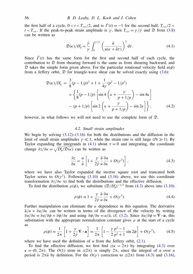
The solutions of (3.12)–(3.16) depend on the particular waveform Γ (t) through D(κ).To gain intuition for the distributions under oscillatory shear, we solve for the simplestpossible waveform: triangle-wave oscillatory shear. Here the waveform is Γ (t)= 1 for


the first half of a cycle, 0< t< Tcyc/2, and is Γ (t)=−1 for the second half, Tcyc/2<t< Tcyc. If the peak-to-peak strain amplitude is γ , then Tcyc = γ /γ and D from (3.8)can be written as

D(κ)/Dr0 =

γ

γ

∫ γ /γ

0

(u

u(κ + uτ)

)2

dτ . (4.1)

Since Γ (t) has the same form for the first and second half of each cycle, thecontribution to D from shearing forward is the same as from shearing backward, andD takes the simple form given above. For the particular rotational velocity field u(φ)from a Jeffery orbit, D for triangle-wave shear can be solved exactly using (3.6):

D(κ)/Dr0 =

38(p− 1/p)2 + 1+ 1

4γ(p2 − 1/p2)

×

18(p− 1/p)

[sin 4

(κ + γ

p+ 1/p

)− sin 4κ

]− (p+ 1/p)

[sin 2

(κ + γ

p+ 1/p

)− sin 2κ

]; (4.2)

however, in what follows we will not need to use the complete form of D.

4.2. Small strain amplitudesWe begin by solving (3.12)–(3.16) for both the distributions and the diffusion in thelimit of small strain amplitudes γ 1, while the strain rate is still large (Pe 1). ByTaylor expanding the integrands in (4.1) about τ = 0 and integrating, the coordinatechange ∂z/∂κ =√Dr

0/D(κ) can be written as

∂z∂κ= u

u

[1+ γ

2γuu∂u∂κ+O(γ 2)

], (4.3)

where we have also Taylor expanded the inverse square root and truncated bothTaylor series to O(γ 2). Following (3.10) and (3.16) above, we use this coordinatetransformation ∂z/∂κ to find both the distributions and the effective diffusion.

To find the distribution ρ(φ), we substitute (D/Dr0)−1/2 from (4.3) above into (3.10):

ρ(φ)∝ 1+ γ

2γuu∂u∂κ+O(γ 2). (4.4)

Further manipulation can eliminate the κ dependence in this equation. The derivativeu/u × ∂u/∂κ can be written in terms of the divergence of the velocity by writing∂u/∂κ = ∂u/∂φ× ∂φ/∂κ and using ∂φ/∂κ = u/u, cf. (3.2). Since ∂u/∂φ=∇ · u, thissubstitution with the appropriate normalization constant gives ρ at the start of a cycleas

ρ(φ)= 12π

[1+ γ

2γ∇ · u

]= 1

2π

[1− γ

2p2 − 1p2 + 1

sin 2φ]+O(γ 2), (4.5)

where we have used the definition of u from the Jeffery orbit, (2.1).To find the effective diffusion, we first find z(κ = 2π) by integrating (4.3) over

κ = (0, 2π). The O(1) term in z(2π) is simply 2π, since the integral of u over aperiod is 2πu by definition. For the O(γ ) correction to z(2π) from (4.3) and (3.16),


10–5

10–6

10–4

10–3

10–2

10–2

10–1

10–1

100

100 101

Simulated

Simulated

(a) (b) (c)

FIGURE 3. (Colour online) Small-amplitude oscillatory shear orientation distributions, forparticles with aspect ratio p= 2.83 at Pe= 104. (a) The distribution ρ(φ) from simulationat a strain amplitude of γ = 0.3. (b) The corrections to the distribution δρ ≡ ρ(φ)− 1/2πas measured from simulation, for strain amplitudes ranging from γ = 0.02 (innermost redcurve) to γ = 2.0 (outermost blue curve), with four curves equally spaced in γ highlightedin black. At amplitudes near γ = 2, higher-order corrections cause the distribution tomove away from 45 extensional axes. The circular gridlines are spaced at separationsof δρ = 0.5/2π, with the second gridline corresponding to δρ = 0; the radial gridlinesare equally spaced in φ. (c) Log–log plot showing the maximal deviation ρ–ρ0 of thesimulated distributions from the zero-amplitude distribution (upper red curve) and themaximal deviation ρ–ρ1 from the first-order correction (lower green curve), as a functionof γ . The second-order corrections are about 20 % of the first-order correction at γ = 1.

the additional integral is ∝∫ 2π

0 (∂u/∂κ) dκ , which is zero since u is periodic in κ .Substituting these values of z(κ = 2π) into (3.16) shows that to O(γ ), the diffusionis not enhanced:

Dreff =Dr

0 +O(γ 2). (4.6)

In the limit of γ → 0, both the distributions and the diffusion remain unchangedfrom their zero-shear value, despite the strain rate dominating over diffusion (γ Dr

0). In this limit, the frequency of the shear is large compared to the rotary diffusion.The distribution remains isotropic because the flow oscillates so rapidly that diffusioncannot alter the distribution at all over a cycle. Similarly, since the portion of theJeffery orbit traversed by a given particle is so small, over one cycle the particle doesnot explore the varying rotary velocities needed to enhance the diffusion. As a result,the diffusion remains at its equilibrium value and is not enhanced.

As γ is increased, the particles start to sample more of the Jeffery orbit. Atthese larger amplitudes, enough of the Jeffery orbit is traversed where it can interactwith diffusion. This interplay results in an O(γ ) correction to the distribution, (4.5).Physically, the form of the distribution arises because the Jeffery orbit starts toalign the distribution. Since the flow oscillates too fast for the distribution to aligncompletely, the result is a partial alignment along the extensional axis, where thestretching due to the Jeffery orbit is largest. Interestingly, this ∝ sin 2φ correction tothe distributions for large Pe and low γ is the same form as the correction to thecontinuous shear distribution at low Pe and large γ , cf. Peterlin (1938), Kim & Fan(1984), Stasiak & Cohen (1987) and Strand et al. (1987). However, this similarity issomewhat coincidental as it depends on the form of u. There is excellent agreementbetween the predictions for the distributions and our simulations, as shown in figure 3.

In contrast, due to symmetry the diffusion constant is only enhanced at O(γ 2),cf. (4.6). The diffusion constant Dr

eff describes the long-time orientation dynamics;


thus Dreff must be symmetric under a reversal in the flow direction. Since reversing

the flow direction corresponds to changing γ → −γ and φ → −φ, Dreff cannot be

enhanced at O(γ ); the quadratic increase of Dreff with γ is shown in the inset to

figure 5(a). The distributions, on the other hand, depend on both γ and φ andtherefore can have an O(γ ) correction while still respecting this symmetry.

4.3. Intermediate resonant amplitudesBy noting other symmetries of oscillatory shear and the Jeffery orbits, we canfind another solution to the oscillatory shear equations. The Jeffery rotary velocityfield repeats itself after half an orbit, as visible from (1.1) and figure 1. Thus, aparticle starting at a given orientation samples the same velocities whether it issheared forwards or backwards for half an orbit. This symmetry is reflected inthe triangle-wave D(κ) in (4.2): at resonant strain amplitudes γr ≡ nπ(p + 1/p)corresponding to half a Jeffery orbit, D(κ) takes its constant continuous shear value.As a result, at half-integer Jeffery orbit amplitudes, triangle-wave oscillatory shearis exactly the same as continuous shear, with the same distributions and diffusionconstant.

Since (3.7) and (4.1) are considerably simplified at resonance under triangle-waveshear, they allow for a perturbative treatment near γr. The procedure is similar tothe low-amplitude strain treatment outlined above, except here the small parameteris the difference δγ from a resonant strain amplitude γr; i.e. γ = γr + δγ . Sinceresonant amplitude shear is similar to continuous shear, the distribution is simplestin the continuous shear coordinate κ . To first order in δγ , the ancillary distributionf (κ) and the diffusion are

f (κ)= 12π

1+ δγ

γr

[λ

1+ λ2/2cos(2κ)− λ2

4(1+ λ2/2)cos(4κ)

]+O(δγ 2), (4.7)

Dreff /D

r0 = 3

8(p− 1/p)2 + 1+O(δγ 2). (4.8)

Like the low-amplitude case, the distributions change to first order in δγ , and thediffusion does not change until O(δγ 2). However, unlike the low-amplitude case, thecorrection to the distribution is not a single harmonic, but it is composed of twoharmonics in the stretched κ-space. These predictions are compared against simulationresults in figure 4 for the distributions and figure 5(a) for the diffusion. While figure 4only compares the simulated and predicted distributions near the first resonant peakfor a single aspect ratio, we find good agreement between (4.7) and (4.8) and thesimulation over a range of both aspect ratios and resonant amplitudes.

4.4. Very large amplitudesSince continuous shear can be thought of as triangle-wave oscillatory shear withinfinite strain amplitude, we expect that at very large amplitudes the distributions onlyvary slightly from the continuous shear distributions. This approach to continuousshear can be seen directly from (4.1) and (4.2). The function D(κ; γ ), whichdetermines both Dr

eff and ρ, is an average value of a periodic function wherethe strain amplitude γ sets the range of the integration. As γ is increased, moreand more periods of the integrand are averaged over, and D(κ) approaches itsinfinite-period average value of the continuous shear Dr

eff from (2.15). In the limit ofinfinite amplitude, the oscillatory shear equation (3.7) becomes the continuous shear


10–2 10–1 100 101

10–5

10–6

10–4

10–3

10–2

10–1

100

Simulated

Simulated

(a) (b) (c)

FIGURE 4. (Colour online) Oscillatory shear orientation distributions for particles withaspect ratio p = 2.83 (i.e. Jeffery orbit period γTJO = 20) at Pe = 104 and a strainamplitude near the first resonance. (a) The ancillary distribution f (κ) from simulation ata strain amplitude of γ = 10.6; note the small bias away from the flow direction. (b) Thedifference between the continuous shear f and that measured from simulation, for positivedistances from resonance δγ = 0 (innermost red curve) to δγ = 1.0 (outermost blue curve),with four curves equally spaced in δγ highlighted in black. The circular gridlines arespaced at intervals of δf = 0.15/2π, with the second gridline corresponding to δf = 0. Theradial gridlines are equally-spaced in φ (not κ). (c) Log–log plot showing the maximaldeviation f –f0 of the ancillary distribution from the continuous shear f (upper red curve)and the maximal deviation f –f1 from the first-order correction (lower green curve), as afunction of δγ . The second-order corrections are about 20 % of the first-order correctionat δγ = 0.4.

equation (2.13). Examining the many-cycle averages in (3.8) shows that the differencebetween D(κ; γ ) and the continuous shear limit decreases as ∼1/γ , which is echoedby the distributions near resonance in (4.7). Both empirically and by analyticallyevaluating the many-cycle averages, we find that Dr

eff approaches its continuous shearvalue like ∼1/γ 2, faster than the distributions do.

4.5. Arbitrary amplitudesThe oscillatory shear equations (3.12)–(3.16) give predictions for Dr

eff and thedistributions at all amplitudes, not just at the ones treated perturbatively above.We find the effective diffusion and distributions at arbitrary amplitudes by evaluating(3.10) and (3.16) numerically for triangle-wave shear. Since oscillatory shear can alsobe used to control the alignment of colloidal rods, we quantify ρ via the liquid crystalscalar order parameter S which captures the degree of total alignment irrespectiveof the direction. The order parameter S is defined as the largest eigenvalue of thetraceless orientation tensor Q; in two dimensions Q is defined as Q = 2〈nn〉 − δ,where δ is the identity tensor and n the orientation unit normal. For an isotropicdistribution, S = 0; for a perfectly aligned distribution, S = 1. Figure 5 comparesthese predicted values (green lines) of Dr

eff , (a), and S, (b), versus γ against thosemeasured from simulation (red dots). We find excellent agreement between thissemi-analytic theory and full numerical simulations for both the diffusion coefficientsand distributions, both for the aspect ratio p = 2.83 shown in figure 5 and overa range of aspect ratios (not shown). The diffusion increases gradually from itszero-amplitude value Dr

eff /Dr0= 1, reaching the continuous shear value at the resonant

amplitude γr. At higher amplitudes, the diffusion undergoes damped oscillations with


0 101.0

1.5

2.0

2.5

3.0

3.5

20 30 40 50 60

0.1

0

0.1

0.2

0.3

0.4

0.5

0.6

10 20 30 40 50 60

0 0

1.00

1.03

0.5 0.5

S

Simulated S

S

Predicted S

(a) (b)

FIGURE 5. (Colour online) (a) Oscillatory shear diffusion Dreff versus γ for particles

with aspect ratio p≈ 2.83, as calculated from (3.16) (green line) and as measured fromsimulation at Pe= 104 (red circles). The results from simulation and from (3.16) are thesame to the resolution of the plot. The oscillations in the diffusion constant with increasingstrain amplitude are clearly visible. Inset: Dr

eff /Dr0 at low amplitudes. (b) The liquid crystal

order parameter S versus γ at the start of a shear cycle for particles p≈ 2.83, as predictedfrom (3.10), green line, and measured from simulation at Pe= 104, red dots. At zero strainamplitude the distribution is randomly aligned (S = 0); with increasing strain amplitudethe distribution becomes more aligned, with maximum alignment at γ = 6. Inset: S at lowamplitudes. In the main panels of both (a) and (b) only 1 % of the simulated points areplotted to avoid overcrowding.

γ , asymptotically approaching its continuous shear value at large strains. In contrast,the order parameter S increases from 0 linearly with γ when γ is small. Moreover,S is not maximal at the resonant amplitudes, but is instead maximal at an amplitudeslightly below the first resonance. The order parameter then decreases slightly to itscontinuous shear value, with damped oscillations at larger γ .

5. Rheology

The orientation distribution of axisymmetric particles affects the suspensionrheology. In the dilute limit, the additional deviatoric stress σ p due to the particles is

σ p = 2ηc

2AH (E : 〈nnnn〉 − δE : 〈nn〉)+ 2BH

(E · 〈nn〉 + 〈nn〉 · E − 2

3δE : 〈nn〉)+ CHE + FHDr

0

(〈nn〉 − 13δ)

(5.1)

where η is the solvent viscosity, c is the volume fraction of particles, E is the far-fieldrate-of-strain tensor of the fluid, δ is the identity tensor, and AH, BH, CH and FH arehydrodynamic coefficients (Jeffery 1922; Batchelor 1970; Hinch & Leal 1972; Brenner1974; Shaqfeh & Fredrickson 1990; Kim & Karrila 2005). The terms ∝E result fromthe additional hydrodynamic resistance due to the particles, which depends on theparticles’ specific orientations through the average tensors 〈nn〉 and 〈nnnn〉. The finalterm ∝ FHDr

0 is an additional stress due to Brownian rotations of the rods. If thedistribution of rods is not isotropic, these Brownian rotations result in a net stress.


As the particle orientations and thus the tensors 〈nn〉 and 〈nnnn〉 couple to theflow, even a dilute suspension of elongated particles has a non-Newtonian rheology.Since 〈nn〉 and 〈nnnn〉 are in general not multiples of the identity, (5.1) genericallypredicts normal stresses. Moreover, both the normal stresses and shear stresses displaytransients before reaching their steady-state values, which in turn depend on the shearrate.

These effects have been well-studied for steady-state distributions, over a range ofPéclet numbers and particle aspect ratios from theory (Peterlin 1938; Leal & Hinch1971; Hinch & Leal 1972; Leal & Hinch 1972; Hinch & Leal 1976; Stasiak & Cohen1987; Strand et al. 1987), experiments (Bibbo, Dinh & Armstrong 1985; Jogun &Zukoski 1999; Brown et al. 2000; Petrich, Cohen & Koch 2000; Chaouche & Koch2001), and simulations (Scheraga 1955; Stewart & Sorensen 1972; Strand et al. 1987).Less is known about the rheology of rod suspensions in time-dependent flows at highPe. Hinch & Leal (1973) made qualitative arguments describing the stress oscillationswith time in a rod suspension; there have also been several simulations of the time-dependent orientation distributions, e.g. Férec et al. (2008) and Eberle et al. (2010),that also examined transient stresses. Our theory of rod dynamics builds on theseresults by providing a quantitative physical picture of the unsteady rheology of asuspension of rods at high Pe, albeit with orientations confined to the flow–gradientplane.

5.1. Rheological transients during startup shearFrom (2.13) and (5.1) we calculate the shear stress of the suspension of ellipsoidalparticles during the startup of shear, for two suspensions with aspect ratios p= 2.83and p= 5.00 at Pe= 104. The orientation distribution starts out isotropically oriented.When the flow starts, the ellipsoids start to tumble in periodic Jeffery orbits, resultingin the large-scale periodic oscillations in the shear stress (figure 6a). These oscillationsslowly damp out with time as the enhanced rotational diffusion brings the orientationdistribution to steady state. Since the diffusion is enhanced ∼p2 for large p, theoscillating stress for p = 5.00 damps faster than the oscillating stress for p = 2.83.At very short times, two additional small peaks in the stress are visible in theseoscillations. However, this stress feature decays extremely rapidly: even at a largePe= 104, it disappears before half a Jeffery orbit for p= 5.00.

To understand the origins of these two types of temporal oscillations in the shearstress shown in figure 6(a), we examine (5.1) term by term. For large shear rates, thelast term ∝Dr

0 is negligible compared to the other terms ∝E , being smaller by a factorof 1/Pe. The third term CHE is independent of time, since the strain rate E is fixed.For orientations confined to the flow–gradient plane, the second term’s contributionto the shear stress is also independent of time, since 2(E · 〈nn〉 + 〈nn〉 · E)xy =〈n2

x + n2y〉 = 1. Thus, at high Pe, only the first term ∝E : 〈nnnn〉 in (5.1) contributes

significantly to the time-dependent shear stress. This term provides an additionalshear stress (〈nnnn〉 : E)xy = 〈1 − cos 4φ〉/8 that is largest at the four orientationsalong the principle strain axes, φ = (n/2 + 1/4)π. Likewise, the stress term isminimal at four orientations that occur when the particle is either aligned with theflow or perpendicular to the flow, φ = nπ/2. Thus the time-varying suspensionstress arises from the interplay between the time-varying distributions and theorientation-dependent stress term (1− cos 4φ)/8.

As discussed in § 2, the evolution of the orientations is simplest in the stretchedcoordinate κ . In this coordinate space, the orientation-dependent stress term (1 −cos 4φ)/8 is bunched in κ and moves with a constant velocity u = γ /(p + 1/p).


00

0

0.20.40.6

00.10.20.3

0.8

10 20 30 40 50

5.0

4.5

4.0

2.5

3.0

3.5

100 101 102

10–6

10–8

10–4

10–2

100

Single peaksDouble peaks

p

(a) (b)

(c)

(d)

FIGURE 6. (Colour online) (a) The additional suspension stress σ pxy/ηcγ under continuous

shear, normalized by the solvent viscosity, shear rate magnitude, and aspect ratio, as afunction of dimensionless time γ t. The stress for two suspensions at Pe= 104 are shown:with aspect ratios p = 2.83 (blue) and p = 5.00 (orange). (b) The orientation-dependentstress term (1− cos 4φ)/8 as a function of κ for p= 5.00. The stress term translates withtime, as shown by the centred bright orange curve at ut= 0 and the shifted drab orangecurve at ut= 0.4π. The double-peaks in the stress term are separated in κ by a distancethat scales as ∼1/p when p is large. (c) The ancillary distribution f (κ), at two times:immediately after startup (black line) and at a time slightly after the double peaks havedisappeared (grey line). (d) The times for the double peaks (magenta) and single peaks(cyan) to decay, as a function of aspect ratio. The decay times follow the ∼1/Dr

0p4 and∼1/Dr

0p2 large-p scalings, respectively, shown in the dotted lines.

The four maximal stress orientations φ = (n/2 + 1/4)π are mapped to κ + ut =tan(±1/p) and tan(±1/p) + π, creating a double-peak in the stress term whoseseparation decreases as 1/p when p is large, cf. (2.2) and figure 6(b). For an initiallyisotropic suspension, the ancillary distribution f (κ) starts out tightly peaked andevolves diffusively to a constant value, figure 6(c). The resulting suspension stressarises from the average of the product of the κ- and t-dependent stress term and thetime-dependent distribution f (κ).

On short times, the ancillary distribution f remains essentially constant while thestress term translates in κ . At time t = 0, the double peaks in the stress term arecentred around the highly peaked initial distribution, which creates a relatively highstress as illustrated by figure 6(a–c). After a short time ∼1/γ , the stress term hasmoved to the left by the small amount ∼1/p, and f centres on one peak of thestress term. This large overlap produces the short-lived increase in the suspensionstress occurring immediately after startup in figure 6(a). At a slightly later time ∼p/γ ,the stress term progresses further to the left by an amount ∼O(1), as shown by thedrab orange curves, and the troughs in the stress term align with the peaks of f (κ),giving rise to the large single troughs in the suspension stress. As the shear continues,the double peak of the stress term moves half a period and realigns with f (κ). Thisrealignment produces the observed double peaks in the stress, and the cycle repeats.

On longer time scales, the enhanced diffusion starts to broaden the ancillarydistribution. As f (κ) broadens, it simultaneously samples multiple regions of theorientation-dependent stress term, and features in σ p

xy(t) start to disappear. The firstto disappear is the double-peak in the suspension stress. When f has broadened bythe ∼1/p separation between the double-peaks in the stress term, figure 6(c), boththe double peaks and the single trough between them are sampled simultaneously,


0

0 2.5 5.03.0

3.2

0

1

2

3

2

–2

–1

–3

4 6 8 10 0 10 20 30 40 50 60 10 20 30 40 50 603.00

3.05

3.10

3.15

3.20

3.25

0

0.03

0.06

0.09

0.12

0.15

First half-cycle

Additional stressIntrinsic viscosity

(a) (b) (c)

FIGURE 7. (Colour online) (a) The normalized additional suspension shear stress σ pxy/ηcγ

as a function of time for triangle-wave oscillatory shear at amplitude γ = 5.0. We definethe effective viscosity [ηeff ] as the average of this varying stress over one cycle (dashedblack line in inset); the additional variation in the stress we quantify by range of thenormalized stress over one half-cycle (grey band in inset). (b) The oscillatory sheareffective viscosity [ηeff ] as a function of γ . (c) The range of the normalized suspensionstress as a function of γ ; it is always small compared to [ηeff ].

and the double-peaks in σ pxy(t) become blurred into a single peak. Diffusion broadens

f (κ) by this ∼1/p amount after a time ∼(1/p)2/Dreff ∼ 1/Dr

0p4 for large p. Even withmoderate aspect ratios at high Pe, the decay of the double-peaks in the suspensionstress onsets extremely quickly: at Pe= 104 and p= 5.0 in figure 6(a), the peaks havedisappeared before the first half Jeffery orbit. Beyond this time scale, the suspensionstress continues to oscillate but only with a single-peaked structure. These singlepeaks in turn disappear after f (κ) broadens by an O(1) amount and samples theentirety of the stress term simultaneously. This O(1) broadening only occurs after amuch longer time ∼1/Dr

eff ∼ 1/Dr0p2 for large p.

The aspect ratio dependence of these two decay times is shown in figure 6(d). Toverify the predicted large aspect ratio scaling, we evaluated the stress from (5.1) usingthe distributions predicted by the continuous shear theory, (2.13) and § 2. We definethe double-peak disappearance time as the time when the stress at a half-integerJeffery orbit switches from a local minimum to a local maximum, and we define thesingle-peak disappearance time as the time when the amplitude of the double-peaksdecays to 1/e of its initial value, as described in detail in appendix B. We find goodagreement between the simulated time scales and those predicted from the scalingargument above (figure 6d). These two time scales ∼1/Dr

0p4 and ∼1/Dr0p2, first

noticed by Hinch & Leal (1973), both arise from the mixing of the phase angle inthe Jeffery orbit. For orientations in three dimensions, there will be additional timescales associated with the relaxation of the orbit constants.

5.2. Overview of triangle-wave oscillatory shear rheology at long times t 1/Dreff

A representative shear stress signal during one cycle of oscillatory shear is plottedin figure 7(a), for spheroids with aspect ratio p = 2.83 and peak-to-peak strainamplitude γ = 5, after f (κ) has reached steady state. Although the transients of theorientation distribution have decayed, ρ still oscillates with the period of one cycle.This oscillation in ρ modulates the stress over one half-cycle (figure 7a inset), andstrictly there is no effective viscosity for a rod-like suspension under oscillatoryshear. Nevertheless, since the variations in the stress are small, it is convenient to


describe the stress response under oscillatory shear with its value averaged overa half-cycle. To this end, we define the ‘effective intrinsic viscosity’ [ηeff ] of thesuspension as the additional shear stress due to the ellipsoids normalized by thesolvent viscosity, particle volume fraction, and shear rate, σ p

xy/(ηcγ ), and averagedover a half-cycle. The slight variation of the suspension stress we quantify by therange of the normalized stress over one-half cycle, shown in figure 7(c).

As is the case for continuous shear, the interplay between the orientation distributionand the stress term (E : nnnn)xy = (1 − cos 4φ)/8 determines the oscillatory shearrheology. However, there are a few differences between the procedure for understandingthe suspension stress under oscillatory shear and under continuous shear. First, thestresses in the first and second half-cycle have the same magnitude, so we onlyexamine the stress during the first half-cycle. Second, since diffusion is weak(Dr

effγ /γ 1), f (κ) is constant throughout a cycle, and only the motion in κ ofthe stress term produces a time-dependent suspension stress. Third, the change inthe long-time f (κ) with strain amplitude effects a change in the suspension stresswith γ . Fourth, due to its amplitude-dependent displacement uγ /γ the motion of thestress term (1 − cos 4φ)/8 produces an additional γ dependence in the suspensionstress. By examining in this way the overlap between the ancillary distribution f (κ)and the orientation-dependent stress term (E : nnnn)xy(κ + ut), we can reconstruct thesuspension stress during one cycle of triangle-wave oscillatory shear and understandthe oscillatory shear rheology shown in figure 7. Rather than laboriously examine eachamplitude in the figure, we now examine three salient amplitude regions of interest:(i) low amplitudes γ 1, (ii) the strain amplitude with the maximal viscosity γ ≈ 1.7,and (iii) amplitudes near resonance γ ≈ γr.

5.3. Low amplitude [ηeff ]For γ → 0, the orientation distribution is isotropic, cf. (4.5), and σ p(t) is the sameas in an isotropic distribution at shear startup. For finite but low amplitudes, thesuspension stress is constant during each half-cycle at O(γ ), figure 8(a). During eachhalf-cycle of shear, the stress term moves by a small displacement ut = uγ /γ , asshown in figure 8(b). In addition, f (κ) shifts from its zero-amplitude value (verticalline) as γ increases, figure 8(c). This shift can be seen from (3.10) and (4.3): f atsmall amplitudes is the first-order term in a Taylor series in γ of an initially isotropicdistribution f0(κ) shifted in κ by half the displacement of the stress term:

f (κ)= f0

(κ + γ u

2γ

)+O(γ 2). (5.2)

Thus, to first order in γ the centre of the stress term oscillates about the centreof f . Since both f and the stress term are constant to first order in κ about theircentres, σ p(t) changes from its zero-amplitude value only at O(γ 2) during the cycle.The displacement of f in κ-space corresponds to a distribution ρ(φ) at the start ofa cycle that is larger along the flow’s compressional axis and is smaller along theextensional axis, reversing as the flow oscillates, cf. figure 3. The increase in the stressfrom orienting particles along the extensional axis at φ=π/4 is exactly cancelled bythe particle reorientation away from the compressional axis.

5.4. Amplitude resulting in maximal [ηeff ]Despite the lack of an exact analytical solution for the distributions at arbitraryamplitudes, we can qualitatively understand the existence of a maximum in [ηeff ].


0

0

0.2 0.4

0.1 0.2 0.33.0

3.1

3.2

3.3

0.6

First half-cycle

0

1

2

3

–2

–1

–3

0

0

0.1

0.2

0.3

0.3

0.6

0

(a) (b)

(c)

FIGURE 8. (Colour online) Low-amplitude γ = 0.3 oscillatory shear rheology for a dilutesuspension of particles with aspect ratio p = 2.83 confined to the flow–gradient plane.(a) The normalized additional suspension stress σ p

xy/η0cγ as a function of dimensionlesstime γ t throughout one cycle of oscillatory shear, with a closeup of the stress duringthe first half cycle in the inset. (b) The orientation-dependent stress term (E : nnnn)xyas a function of κ . The stress term starts with its minimum centred at κ = 0, shownas the centred (right) curve in light blue. During the cycle, the Jeffery orbit advects thestress term through the lightly shaded region. At the end of the half-cycle, the stress termreaches its final position, shown as the shifted (left) curve in dark blue. (c) The ancillarydistribution f (κ). The shaded region denotes the area swept out by the centre of the stressterm. The peak of f (κ) is shifted from κ = 0 to the centre of the region that the stressterm sweeps out during a cycle.

As shown above, for small amplitudes f (κ) shifts as γ increases but is otherwiseunchanged. This shift suggests a mechanism for the maximal [ηeff ]. As f (κ) is shiftedby a larger amount, eventually its peak is centred on one peak in the stress term,producing a large suspension stress at the cycle’s start. During the cycle, the stressterm translates until its trough and then second peak overlap with f , creating firsta slightly lower stress before another large stress again at the end of the half-cycle,similar to the double-peaks in the stress under continuous shear. This translation off corresponds to a distribution ρ(φ) that is isotropic at the centre of the cycle, butis nonlinearly distorted by the Jeffery orbit to orient more particles along the flow’sextensional axis than are removed from the compressional axis, cf. the γ ≈ 2 contoursin figure 3. This double-peak structure in the suspension stress and the shifted f (κ)are borne out in figure 9(a,b). Since σ p(t) increases at the ends of the cycle, [ηeff ]increases from its zero-amplitude value, and the range of the stress is non-zero. Whilethe argument captures the essence of the occurrence of a maximal viscosity, there arehigher-order corrections in γ to f that cause the suspension stress to deviate slightlyfrom the expected results.

The argument above suggests a scaling with aspect ratio for the strain amplituderesulting in a maximal viscosity. As visible from the definition of κ in (2.3), theseparation between the double-peaks in the stress term scales as ∼1/p for large p.From (5.2), the small-amplitude correction to the ancillary distribution shifts f by anamount ∼γ /p, since u/γ = 1/(p+ 1/p). Thus, at a strain amplitude γ ∼ 1 independentof p, the peak of f is roughly centred on one of the peaks in the stress term. Asa result, the amplitude producing the maximal viscosity should be independent ofthe particle aspect ratio p. This prediction is verified in figure 9(d). The amplitude


0 0.85 1.701.60

1.70

1.75

1.650 0.85 1.70

2.55 3.40

0

1

2

3

–2

–1

–3

3.0

3.1

3.2

3.3First half-cycle

0

0.3

0.60

0.1

0.2

0.3

0

(b)

(c)

(a)

100 101 102

p

(d)

FIGURE 9. (Colour online) Oscillatory shear rheology at the strain amplitude γ = 1.67resulting in maximal viscosity for a dilute suspension of particles with aspect ratiop = 2.83. (a) The additional suspension stress as a function of dimensionless time γ tthroughout the cycle. (b) The stress term (E : nnnn)xy as a function of κ . The stress termstarts with its minimum centred at κ = 0, shown as the centred (right) curve in light blue.During the first half-cycle, the Jeffery orbit advects the stress term through the lightlyshaded region until it reaches final position, shown as the shifted (left) curve in dark blue.(c) The ancillary distribution f (κ); the shaded region denotes the area swept out by thecentre of the stress term. (d) Semi-log plot of the strain amplitude resulting in the maximalviscosity versus p.

resulting in the maximal viscosity is practically constant with p, varying by less than10 % from γ ≈ 1.6 at an aspect ratio p= 2 to its asymptotic value γ ≈ 1.74 at p= 100.

5.5. Resonant amplitude [ηeff ]For resonant amplitudes γ = γr corresponding to half a Jeffery orbit period, theancillary distribution does not vary with κ: f (κ) = 1/2π. As the stress term movesduring the cycle, its overlap with the constant f does not change, and the suspensionstress remains constant during the cycle. A constant f (κ) corresponds to a distributionρ(φ) that does not change with time due to the Jeffery orbit, resulting in a suspensionstress that is constant during a cycle. Thus, the resonant f (κ) yields the samesuspension stress and [ηeff ] as for continuous shear at long times.

For amplitudes slightly away from resonance γ = γr + δγ , the suspension stresschanges at O(δγ ), as shown in figure 10. The first-order correction to f (κ) indicatesthat additional particles are oriented along the maximal stress directions. As a result,the suspension stress at the start of a cycle for amplitudes near resonance is O(δγ )larger than the suspension stress at resonant amplitudes γr. As the stress term moves,at the centre of the cycle it centres on regions where f (κ) is less than its resonant-amplitude value, which decreases the suspension stress. Thus, the range of the stressincreases linearly with δγ , figure 7(c). However, since the effective intrinsic viscosity[ηeff ] is an average of the suspension stress, the oscillations during one half-cyclecancel out, and [ηeff ] remains the same as at resonance, as shown by the smoothminima in figure 7(b).

6. Conclusion and discussionIn the preceding pages, we have solved for the time-dependent orientation

distribution of rod-like particles under shear. Under continuous shear, the convection–diffusion equation is greatly simplified by a change of coordinates φ → κ that


0 5.0 10.0

0 5.0 10.6

15.0 21.2

0

1

2

3

–2

–1

–3

3.0

3.1

3.2

3.3First half-cycle

0

0.3

0.6

0

0.1

0.2

0.3

0

(b)

(c)

(a)

FIGURE 10. (Colour online) Oscillatory shear rheology for an aspect ratio p= 2.83 andan amplitude γ = 10.6 slightly above resonance. (a) The normalized additional suspensionstress σ p

xy/η0cγ as a function of dimensionless time γ t throughout one cycle of oscillatoryshear. (b) (E :nnnn)xy as a function of κ . The stress term starts with its minimum centredat κ = 0, shown as the centred (right) curve in light blue, and is advected by the Jefferyorbit through the lightly shaded region. Since γ = 10.6 is slightly above resonance, thestress term translates by more than half a period and ends at the final position shown asthe shifted (left) curve in dark blue. (c) The ancillary distribution f (κ). The shaded regiondenotes the area swept out by the centre of the stress term, with the darkly shaded regionillustrating the regions where the minimum in the stress term has traversed twice.

removes the rotation of the Jeffery orbit. This coordinate transformation complicatesthe diffusion term, but allows it to be treated perturbatively with a method ofaverages, similar to that used for certain nonlinear ordinary differential equations(Sanders, Verhulst & Murdock 2000) or for homogenization methods for effectivemedium properties (Bakhvalov & Panasenko 1989; Cioranescu & Donato 1999).The convection–diffusion equation cleanly maps to a simple diffusion equationin the new coordinate, with an enhanced diffusion that depends on averages ofthe rotational velocity field: Dr

eff = Dr0〈(u/u)2〉. For particles rotating in a Jeffery

orbit, the diffusion under continuous shear is enhanced as ∼p2 when p is large.Since the orientation dynamics are an exact diffusion equation in the stretchedκ-coordinate at high Pe, a complete solution for any initial distribution can be easilyconstructed, and all initial distributions relax to a constant ancillary distribution in theκ-coordinate. This steady-state ancillary distribution is the two-dimensional analogueof the three-dimensional steady-state solution found by Leal & Hinch (1971).

Under oscillatory shear, a particle does not sample all orientations during eachcycle. As a result, the effective diffusion in the κ-coordinate is an average overthe regions the particle does sample, instead of an average over the entire Jefferyorbit. Since different particles sample different regions during a cycle, the effectivediffusion changes with orientation κ . This varying diffusion causes particles todrift away from the continuous shear distribution, changing f from its continuousshear form. As a result of the orientationally-dependent diffusion, the orientationdynamics in κ-space become complicated. However, it is always possible to mapthe κ-dynamics under oscillatory shear to a simple diffusion equation in a newcoordinate z. Once this mapping is known, a full time-dependent solution for thedistributions under oscillatory shear is easily constructed. While the coordinatechange κ→ z cannot in general be solved analytically, it can be treated perturbativelyat certain amplitudes, particularly for triangle-wave shear, or solved numerically. The


solutions for triangle-wave shear show that, for small strain amplitudes γ 1, theorientation distribution remains isotropic and the rotational diffusion is not enhanced.Moreover, the distributions when γ 1 at large Pe take the same form as thedistributions when Pe 1 at large γ . At resonant amplitudes corresponding tohalf-integer Jeffery orbits, the orientation dynamics map exactly to the continuousshear orientation dynamics, providing the same effective diffusion constant andorientation distribution.

Since the moments of the orientation distribution determine the suspension rheology,the solutions for the orientation distributions allow for a detailed understandingof the suspension shear stresses. Examining the time evolution of the overlapbetween the orientation-dependent stress term E : nnnn and the ancillary distributionf (κ) quantitatively explains all the features in both the continuous and oscillatoryshear suspension rheology. In particular, our formalism demonstrates the existenceof two diffusive time scales in the continuous shear rheology, and predicts anamplitude-dependent effective intrinsic viscosity under oscillatory shear.

6.1. Comparison to Taylor dispersionOur approach of mapping the rod dynamics to an effective diffusion equation isreminiscent of Taylor dispersion. The canonical Taylor dispersion was calculated byTaylor for Poiseuille flow in a circular pipe (Taylor 1953, 1954). As the non-uniformflow in the pipe moves different solute parcels at different speeds, the solutespreads out along the axial direction while diffusion erases the flow-induced radialinhomogeneity. Taylor realized that this combination of diffusion and differentialadvection maps to a simple diffusion equation along the pipe’s axis, with a greatlyenhanced effective diffusion constant. This result is reminiscent of the rotationaldynamics discussed above: the combination of diffusion and differential rotation dueto the Jeffery orbit maps to a simple diffusion equation. A natural question to ask iswhether the enhanced rotational diffusion is simply a modified Taylor dispersion, orwhether it is only similar.

The most general formulation of Taylor dispersion was realized by Howard Brennerand others in the 1980s (Frankel & Brenner 1989). He viewed the essence of Taylor’smethod as examining long times where the distribution is equilibrated in a smallsubspace q (e.g. the cross-section of the pipe) to allow for simple calculationsof behaviour in other, larger subspaces Q (e.g. along the axis of the pipe). Thisabstraction of Taylor dispersion to arbitrary spaces allows for a rigorous, cleancalculation of long-time behaviours. In addition to describing the original Taylordispersion problem, Brenner and others used this insight to understand the dynamicsof seemingly disparate systems, such as the sedimentation velocity of a non-sphericalparticle (Brenner 1979) or of a cluster of particles (Brenner, Nadim & Haber 1987),as well as for more intractable problems such as Brownian motion of particles undershear flow (Leighton 1989; Frankel & Brenner 1991, 1993).

However, the orientation dynamics described in the current paper do not fit simplyinto the canonical generalized Taylor dispersion picture. In the generalized Taylordispersion picture, there are two separate positional subspaces q and Q. In therotational dynamics calculated in this paper, there is only one positional subspace,corresponding to the angular coordinate φ or κ . Thus, Brenner’s approach will notwork for the problem of rotational diffusion. In part, this limitation arises fromthe nature of the rotary velocity field and the diffusion. In Taylor dispersion, theenhanced diffusion arises from Brownian motion perpendicular to the rotary velocity


field. In the enhanced rotational diffusion calculated here, the enhancement arisesfrom Brownian motion parallel to the rotary velocity field, and the varying velocityalong the streamline enhances the rotational diffusion. In contrast, in traditionalTaylor dispersion diffusion parallel to streamlines does not enhance dispersion, sincethe fluid flow is presumed incompressible.

While our analysis for the evolution of the orientation distribution equations doesnot fit neatly into Brenner’s generalized Taylor dispersion, there are still somemathematical similarities between the two. Instead of integrating over a smallpositional subspace q, the analysis in this paper proceeds by integrating over ashort time, either one period of a Jeffery orbit or one oscillatory cycle. It is this stepthat allows for a mapping to a diffusion equation, as it is the small subspace stepthat allows generalized Taylor dispersion to map complicated dynamics to simplerequations.

6.2. Applicability to particle orientations in three dimensionsThe analysis presented above is for particle orientations confined to the flow–gradientplane. A natural question to ask is how relevant these results are for real particleorientations in three dimensions. Previous work by Hinch & Leal (1973) hasinvestigated theoretically how the orientation dynamics of a suspension of rod-likeparticles changes due to shear. While the analysis of the full three-dimensionalproblem proved intractable, they were able to make scaling arguments based ongeneric properties of the orthogonal eigenfunctions of the convection–diffusionoperator. From these arguments, they surmised that there were two time scalesin the orientation dynamics: a ∼1/Dr

0p2 time for the orbit constant relaxation anda ∼1/Dr

0p4 time for the phase-angle relaxation. In § 5, we find the same two timescales for the orientation dynamics in the continuous shear rheology but strictlyfor the phase-angle relaxation, as the orbit constant is fixed for particles in theflow–gradient plane. There is one time scale, ∼1/Dr

0p2, for the phase angle to relaxover the full range of the κ-coordinate. However, a secondary time scale ∼1/Dr

0p4 isproduced since the κ-coordinate stretches the φ-coordinate by an amount ∼p near theflow direction. Thus, our solution shows there are two time scales in the phase-angledynamics, instead of the one suggested by Hinch & Leal (1973). This nuance in thetwo-dimensional dynamics suggests that a full solution for freely rotating particleswould provide additional insight into the orientation dynamics.

When the orientations are not confined to the flow–gradient plane, diffusionrandomizes both the Jeffery orbit’s phase angle and its orbit constant. If the orbitconstant is fixed, diffusion randomizes the phase angle via the same mechanismdescribed in this paper for particles confined to the flow–gradient plane. Indeed,simply substituting the Jeffery orbit velocity u for a fixed orbit constant into (2.13)provides an effective phase-angle diffusion for any Jeffery orbit. It might be hopedthat a full three-dimensional solution could be created by combining this enhancedphase-angle diffusion with a diffusive mixing among orbit constants. However, (1.2)shows that, for large p, the distance between two Jeffery orbits decreases near the flowdirection by a factor ∼1/p compared with their distance near the gradient direction.This bunching of orbit constants results in an enhanced orbit constant diffusion thatincreases with p, creating an additional set of time scales for diffusion across orbits.Moreover, the diffusion across orbit constants could be coupled to the diffusion alongan orbit, preventing a simple piecewise analysis.

To test the relevance of our predictions to three-dimensional orientations, we haveexplored the suspension rheology through a Langevin simulation of three-dimensional


0 10 20 30 40 50

0 200 400 600 800 1000

4.05.0

2.0

6.0

3.0

7.0

3.03.2

2.6

3.4

2.8

3.6

100 101

100 101

10–1

10–2

10–1

10–2

10–3

100

Single peaksDouble peaks

Orbit constants

p

(a)

(b)

(c)

(d)

FIGURE 11. (Colour online) Rheology of a suspension of rod-like particles withorientations allowed to rotate freely in three dimensions, for particle aspect ratios p= 2.83and p= 5.00 and Pe= 104, drawn from two separate initial distributions: (a) equilibratedorbit constant but a single phase angle, and (b) equilibrated phase angle but single orbitconstant. Note the difference in scale for both axes. (c) The decay times of the single-and double-peak structures in the suspension stress, from simulations over a range ofaspect ratios. Since the double-peak structure decays extremely rapidly, our simulationcannot resolve the double-peak decay time for the last two aspect ratios p≈ 7 and p≈ 8.(d) The decay time of the suspension stress at intermediate times due to the orbit constantrelaxation, as a fit over the shaded time window in (b).

particle orientations under continuous shear. As discussed above, there should be twosets of time scales in the suspension rheology: one set for the phase-angle relaxation,discussed in § 5, and a second set of time scales for the orbit constant relaxation.To discern the origins of the simulated rheology time scales, we ran two sets ofLangevin simulations with initial particle orientations (θ, φ) drawn from two separatedistributions.

The first set of simulations consists of particles drawn from an initial distributionwith an equilibrated orbit constant, but with a single phase angle in the flow–vorticityplane (i.e. from the steady-state distribution in Leal & Hinch 1971 with φ restricted toπ/2). Since the orbit constants start completely relaxed, any change in the suspensionrheology arises solely from the phase-angle dynamics. The suspension rheology forthis initial distribution is shown for two aspect ratios p=2.83 and p=5.00 at Pe=104

in figure 11(a). The qualitative features of the suspension shear stress are the same asfor the two-dimensional continuous shear rheology in figure 6(a). There is a distinctdouble-peak structure in the suspension stress for both aspect ratios at short times. Atslightly longer times, the double-peaks fade into single peaks with a period of one-halfa Jeffery orbit. These single peaks appear to decay more slowly. Note that, since theinitial distribution starts from a single phase angle, the double-peaks in the suspensionstress start more pronounced than for the initially isotropic distribution in figure 6(a).

The second set of simulations consists of particles drawn from an initial distributionwith an equilibrated phase angle, but with a single orbit constant in the flow–gradientplane (i.e. θ = π/2 but φ drawn from the continuous shear distribution in (2.14)).Since the phase angle starts completely relaxed, any change in the suspension rheologyarises solely from the diffusive relaxation of the orbit constant. The suspensionrheology for this initial distribution is shown for two aspect ratios p = 2.83 and


p= 5.00 at Pe= 104 in figure 11(b). Since the phase angle starts completely relaxed,the suspension rheology does not change on the time scale of the Jeffery orbit.Instead, the suspension stress only changes on the much longer diffusive time for theorbit constant relaxation, decaying monotonically to its steady-state value.

These time scales for the rheology are shown over a range of aspect ratios infigure 11(c,d). The time scales are extracted from Langevin simulations of 4000particles at Pe = 104, as described in appendix B. The two phase-angle time scalesare defined similarly to those in § 5. The orbit constant time scales shown are definedby fitting the stress at intermediate times to an exponential decay. If the picture forphase-angle dynamics laid out in this paper is relevant for three dimensions, thenfor large p the double-peak should decay quickly on a time scale of ∼1/Dr

0p4 whilethe single peak should decay more slowly on a time scale of ∼1/Dr

0p2. To checkfor this dependence we plot these two time scales for the phase-angle relaxationas a function of aspect ratio on a log–log scale in figure 11(c). There are clearlytwo separate aspect ratio dependences for the two phase-angle time scales, whichseem to be consistent over the limited range with the ∼1/Dr

0p4 and ∼1/Dr0p2 scaling

for particles confined to the flow–gradient plane. Thus the two-dimensional analysispresented in this paper captures much of the three-dimensional orientation dynamics.The decay of the stress due to the orbit constants also shows a time scale that scaleswith p. By fitting the simulated suspension stress to an exponential decay, we findthat the orbit constant relaxation time scale is consistent with the 1/Dr

0p2 scale arguedby Hinch & Leal (1973). These orbit constant time scales are similar in magnitudeto the phase-angle time scales, suggesting that the distribution’s for freely-rotatingparticles is strongly affected by diffusion both along and across orbits.

Under oscillatory shear, we also expect qualitative features of the two-dimensionalsolutions to be present in three dimensions. As shown by Leahy et al. (2013), in threedimensions the orientation distributions change with strain amplitude under oscillatoryshear in a manner similar to the two-dimensional oscillatory shear distributions in § 4.The oscillatory shear diffusion Dr

eff as measured from correlations in three dimensionsalso showed oscillations at the resonant Jeffery orbit amplitudes. Thus, the qualitativefeatures of orientation dynamics for particles confined to the flow–gradient plane arepresent for the full three-dimensional dynamics under oscillatory shear.

6.3. Proposed experiments and possible applicationsThe results presented above suggest several experiments that are possible with currentparticle synthesis techniques. The detailed predictions in this manuscript could betested by confining particles to rotate in a single Jeffery orbits, preferably in theflow–gradient plane. This confinement could be accomplished either via a magneticfield (Almog & Frankel 1995) or by shearing particles adsorbed to a liquid–liquidinterface (Stancik et al. 2003). Moreover, as discussed in § 6.2 many of the scalingsand qualitative predictions of this paper should be relevant for particles rotating inthree dimensions. Precise single-particle measurements via confocal or holographicmicroscopy of Dr

eff over a range of aspect ratios and strain amplitudes could furtherverify the orientation dynamics described above. Alternatively, the average degreeof alignment of an anisotropic particle suspension under oscillatory shear could bemeasured with flow dichroism or a similar technique. Our rheological predictionscould be most easily checked for [ηeff ] as a function of γ , as this measurementallows averaging the stress signal over many cycles to reduce noise. Moreover, thestrain amplitude at which [ηeff ] is maximal is roughly independent of p and thus willbe robust to a suspension with aspect ratio polydispersity.


Our results could also be extended to other regimes and applications. Sincethe analysis in §§ 2 and 3 does not depend on the details of the Jeffery orbit, itcould be easily extended to velocity fields other than a Jeffery orbit, such as forweakly inertial particles (Subramanian & Koch 2005) or for particles in weaklynon-Newtonian suspending fluids (Leal 1975, 1980; Stover & Cohen 1990; Iso,Cohen & Koch 1996a,b). On a practical level, oscillatory shear could be used toalign rod suspensions for colloidal self-assembly or for three-dimensional printedinks with fibres embedded in them (Shofner et al. 2003; Compton & Lewis 2014).As shown in figure 5(b), the maximal orientational alignment is not obtained undercontinuous shear but is at a resonant amplitude that depends on the aspect ratio. Byusing the arbitrary-waveform oscillatory shear equations (3.7) and (3.8), it might bepossible to design a specific waveform for a desired degree of particle alignment.Over ninety years after Jeffery’s solution for particle rotations in a viscous fluid,rod-like particles still have intellectually interesting and practically applicable featuresworthy of discovery.

AcknowledgementsWe would like to thank L. Bartell, T. Beatus, and J. Sethna for useful discussions.

We acknowledge support from the National Science Foundation (CBET-1435013)(D.L.K.), from the US Department of Energy, Office of Basic Energy Sciences,Division of Materials Science and Engineering under Award No. ER46517 (I.C.), andfrom National Defense Science and Engineering Graduate (NDSEG) Fellowship 32CFR 168a (B.D.L.).

Appendix A. Continuous and oscillatory shear numerical solutionsA.1. Continuous shear simulation

We numerically solved the Fokker–Planck equation for the distribution’s time evolution(2.1) by expanding the distribution ρ in Fourier space and transforming (2.1) intoa sparse matrix equation. For our simulations, we truncated the Fourier series tothe first 301 terms (i.e. m ∈ [−150, 150] for basis functions eimφ); the resultingcoupled ordinary differential equations were solved with a fourth-order Runge–Kuttaintegration scheme with a time step of dt=5×10−4/γ . Either increasing or decreasingthe number of terms or the time step had little effect on the simulation results.Rather than simulate a specific set of initial conditions, we evolve 301 separate initialconditions corresponding to ρm(φ, t = 0)= eimφ . Using the linearity of (2.1), we canthen reconstruct an arbitrary distribution from this set of initial distributions. Wecan also use these simulation results to rapidly numerically solve for triangle-waveoscillatory shear, as described below.

A.2. Construction of oscillatory shear propagatorsRather than numerically integrate (3.1) for triangle-wave oscillatory shear at eachstrain amplitude, we instead opted to numerically create a set of oscillatoryshear propagators and find the oscillatory distribution from these propagators. Thepropagators can be constructed rapidly from the continuous shear solutions and allowfor rapid evaluation of the oscillatory shear distributions after an arbitrary time.

To find these propagators, we first find the change in ρ after one full cycle fromthe continuous shear simulations. One cycle of triangle-wave oscillatory shear canbe viewed as two separate pieces: continuous shear going forward for a time γ /γ ,


followed by continuous shear going backward for the same time. Let the probabilitydistribution ρF = ρF(φ, t | φ0) be the probability density of finding a particle withorientation φ after undergoing forward shear for a time t, given that the particle startedat an orientation φ0. Similarly, let ρB(φ, t | φ0) be the probability density of finding aparticle at orientation φ after undergoing backward shear for a time t. The orientationof the particle φ after a full cycle is a two-step process: after the first half of acycle, the particle rotates to an intermediate orientation φ1/2 with some probabilityρF(φ1/2, t= Tcyc/2 | φ0), then rotates during the second half of the cycle from φ1/2 toits final orientation φ1 with some other probability ρB(φ1, t | φ1/2). We integrate overφ1/2 to find the conditional probability distribution ρ(φ1, t= Tcyc | φ0) of the particle’sfinal orientation after a full cycle:

ρ(φ1, Tcyc | φ0)=∫ρF(φ1/2, Tcyc/2 | φ0)ρB(φ1, Tcyc/2 | φ1/2) dφ1/2. (A 1)

Now, we Fourier expand ρF(φ1/2, Tcyc/2 | φ0) in both φ1/2 and φ0, and similarly forρB:

ρF(φ1/2, Tcyc/2 | φ0)=∑

kl

AFkle

ikφ1/2eilφ0, (A 2)

ρB(φ1, Tcyc/2 | φ1/2)=∑

mn

ABmneimφ1einφ1/2 . (A 3)

Substituting into (A 1) and integrating gives a Fourier expansion of ρ(φ1, Tcyc |φ0) as

ρ(φ1, Tcyc | φ0)=∑

ml

B1mle

imφ1eilφ0,

where B1ml ≡ 2π

∑n

AF−n,l AB

mn.

(A 4)

Thus, we can calculate the distribution after one cycle of triangle-wave oscillatoryshear from the continuous shear distributions by using matrix multiplication. Incontrast, most other waveforms require a full numerical solution for ρ at each strainamplitude.

To find the distribution after N + 1 cycles, we follow a similar argument. We canview the probability of finding the particle at an orientation φN+1 after N + 1 cyclesas a two-step process: the particle started at φ0 and rotated to φN after N cycleswith some probability ρ(φN,NTcyc | φ0), followed by a rotation from φN to φN+1 withprobability ρ(φN+1, Tcyc | φN) after the final cycle. Following the same argument asabove, the distribution ρ(φN+1, (N + 1)Tcyc | φ0) can be written as

ρ(φN+1, (N + 1)Tcyc | φ0)=∑

lm

BN+1ml eimφN+1eilφ0,

where BN+1ml ≡ 2π

∑n

BN−n,lB

1mn.

(A 5)

Thus the distribution after an arbitrary number of triangle-wave oscillation cycles canbe reconstructed from the simulated forward and backward probability distributions,once the coefficients AF

kl, ABmn are known.

The coefficient matrices AFkl,A

Bmn can in turn be calculated from the continuous shear

solutions. Letρk(φ, t)=

∑l

akl(t)eilφ (A 6)


be the continuous shear solution of (2.1) subject to the initial condition ρk(φ, 0)= eikφ ,i.e. akl(0)= δkl. Due to linearity, any distribution ρ(φ, t) can be written as a sum overthe ρk. In particular, we can write ρF(φ, t | φ0) in this way:

ρF(φ, t | φ0)=∑

k

qk(φ0)ρk(φ, Tcyc/2), (A 7)

where qk(φ0) are the coefficients of the Fourier expansion whose values depend on φ0.Substituting the definition of ρk ≡

∑k akleilφ , we can write this as

ρF(φ, t | φ0) =∑

k

qk(φ0)∑

l

akl(t)eilφ

=∑

kl

qk(φ0)akl(t)eilφ. (A 8)

The distribution ρ(φ, t | φ0) is defined such that ρ(φ, 0 | φ0) = δ(φ − φ0) ≡(1/2π)

∑kexp(ik(φ − φ0)). Substituting this into (A 8) at t = 0 and using the

definition of AFkl from (A 2), the forward shear propagator AF

kl and the continuousshear coefficients akl can be related as

AFkl =

12π

a−l,k(Tcyc/2). (A 9)

To obtain the coefficients for backward shear ABkl, we note that shearing backwards is

the same as taking φ→−φ, φ0→−φ0, as visible from (2.1). This is in turn the sameas switching the signs of the indices, so the backward shear propagator AB

kl is

ABkl =

12π

al,−k. (A 10)

Thus, from our simulation for continuous shear in one direction only, we can quicklyrecreate the time-dependent distribution ρ under triangle-wave oscillatory shearfor strains of arbitrary amplitude. This same procedure can be used to solve theconvection–diffusion equation after a time t in O(ln t) steps instead of the normalO(t) steps needed for direct numerical integration; we use this procedure to rapidlyfind the long-time distributions under oscillatory shear. We used this fast method tofind both ρ and Dr

eff numerically at ≈3000 separate amplitudes, equally spaced fromγ = 0.02 to 60.00.

A.3. Extracting diffusion constants from simulationFor continuous shear, the diffusion coefficients shown in figure 2 were calculated byfitting exponentials to correlations 〈cos m(κ − κ0)〉 from 20 separate initial orientationsκ0 which were sampled from the steady-state distributions. As mentioned in the text,the fitted correlations in κ-space are independent of the starting orientation, while thecorrelations in the unstretched φ-space do depend on the starting orientation.

For oscillatory shear, the situation is slightly more complicated since the orientationsare diffusive in a new, stretched z-space. Rather than fitting correlations in the newz-coordinate, which must be computed for each strain amplitude, we examine thelong-time decay of an arbitrary correlation. Since the ancillary distribution g(z)


evolves according to a diffusion equation in z-space with an effective diffusion Dreff ,

any correlation C(1t) will decay as a sum of exponentials:

C(1t)=∑

m

Cmexp(−m2Dreff1t). (A 11)

At long times Dreff1t 1, only the term with the smallest m (m = 1) remains; the

others have decayed. To find the effective diffusion under oscillatory shear, weexamine the decay of a correlation C after a long time such that C(t) ∼ 10−3. Fordiffusive correlations, the further decay is entirely due to the m= 1 term; the termsm= 2 and higher are exponentially smaller, approximately C4∼ 10−12 as can be seenfrom (A 11), and do not contribute to the decay. From these long time decays ofthe correlation C, we extract the oscillatory shear diffusion constant Dr

eff . To checkthe robustness of this technique, we evaluate two separate correlations, 〈cos1φ〉 and〈cos1κ〉, for 20 separate initial orientations sampled from the long-time distribution.Empirically, the value of Dr

eff obtained from the long-time correlations is independentof either the particle’s starting orientation or the type of correlation fitted. In contrast,at short and intermediate times the extracted Dr

eff varies with both the initial particleorientation and the type of correlation fitted. This difference at short times arisesbecause the orientation is in general not diffusive in either the original φ-space orthe continuous shear stretched κ-space, but is diffusive in the (uncalculated) z-spacefor oscillatory shear.

Appendix B. Rheology calculations and rheological time scale definitions

Calculating the rheology. To calculate the suspension rheology for the two-dimensionalparticle orientations under continuous shear, we used the theory of two-dimensionalrod dynamics presented in § 2 to find the time-dependent ancillary distribution f (κ, t)at Pe = 104. Once the ancillary distribution is known, the suspension stress canbe calculated from (5.1). To find the rheology for orientations in three dimensions,we numerically integrated a Langevin equation for 4000 separate initial particleorientations at Pe = 104, by integrating (1.1) with an additional noise term using anEuler method. The time step size dt= 5× 10−4/γ gives an integration error after eachtime step that is 10−3 that of the random motion. The orientation moment tensors〈nn〉 and 〈nnnn〉 are evaluated from direct averages of the particle orientations.

To calculate the triangle-wave oscillatory shear rheology for two-dimensionalparticle orientations, we first obtained the oscillatory shear distributions at longtimes. The ancillary distribution f (κ) can be found from (3.10). While the coordinatederivative ∂z/∂κ and thus the functional form of f can be exactly evaluated analyt-ically, the distribution’s normalization must be evaluated numerically. Alternatively,the distribution ρ can be found from the simulations at Pe= 104; we find that bothprocedures produce the same rheology to within ≈1/Pe. To find the stress duringone half-cycle, we evolved the distributions in the limit of no diffusion for theduration of the half-cycle; since our theory describes the limit of large strain ratesthe ancillary distribution does not diffusively evolve during a cycle. The maximal[ηeff ] amplitudes are found only from (3.10) which is orders of magnitude faster thansimulating the orientation distributions; we use a Nelder–Mead simplex algorithm tofind the maximal [ηeff ] amplitudes for the 1000 aspect ratios logarithmically spacedfrom p= 1.5 to 100.0 shown in figure 9(c).


Definitions of rheological time scales. The double-peak decay time scale in figure 6(c)is defined as the time when the suspension stress at half-integer Jeffery orbits switchesfrom a local minimum to a local maximum. To find this time scale, we examinedthe second derivative of the suspension stress via our analytical solution after a fixedtime corresponding to 200 half-integer Jeffery orbits and varied the rotary diffusionDr

0. Examining the stress after these long times prevents the decaying envelope of thesuspension stress from biasing the second derivative. Traces of the single peaks arealways present, in contrast to the double-peaks which completely disappear after awell-defined time. To minimize short-time transients in the single peak decay time, welooked for the time when the magnitude of the single peaks decayed to 1 % of theirinitial value, by examining the stress at a fixed time corresponding to the first troughafter 200 half-integer Jeffery orbits (i.e. γ t= 200.5π(p+ 1/p)) and varying Dr

0. Sincethe double-peak structure obscures the height of the suspension stress’s initial peak att= 0, we examine the decay of the minimum of the troughs in the stress, occurringevery (n+ 1/2)/2 Jeffery orbits. We then rescaled this time to give the corresponding1/e decay time of the single peaks.

We extracted the double-peak and single-peak decay times for the three-dimensionalsuspension rheology in a similar manner. However, since there is no closed-formsolution for three-dimensional rod orientations, we looked at a single set ofsimulations at Pe= 104 for each aspect ratio and initial distribution. The double-peakdecay time shown in figure 11(c) is the time at which the (smoothed) secondderivative of the stress at each half-integer Jeffery orbit is zero, interpolated betweenhalf-integer Jeffery orbits to improve temporal resolution. For all but the lowest aspectratios, this zero occurs after only a few half Jeffery orbits. The single-peak decaytimes are measured from the same set of simulations. To minimize the effects ofnoise inherent in a Langevin simulation, we calculated the 1/e decay time for thethree-dimensional orientations from when the troughs in the stress decayed to 10 %of their initial value, instead of 1 %.

The orbit constant decay times shown in figure 11(d) are also taken from a singleset of simulations for each aspect ratio at Pe = 104. We defined the time scale forthe orbit constant decay by fitting the shear stress at times 0.06 < Dr

0t < 0.1 to anexponential decay, after subtracting off the steady-state shear stress. To minimize theeffects of noise inherent in the Langevin simulation, we smoothed the simulated shearstress by convolving with a boxcar filter with a width of half a Jeffery orbit; thedata shown in figure 11(b) are not smoothed. While there are some transients in thesuspension stress at shorter times, empirically we find that the suspension stress iswell-described by an exponential decay for all the aspect ratios measured, within thelimited resolution of our simulations.

REFERENCES

ALMOG, Y. & FRANKEL, I. 1995 The motion of axisymmetric dipolar particles in homogeneousshear flow. J. Fluid Mech. 289, 243–261.

BAKHVALOV, N. & PANASENKO, G. 1989 Homogenisation: Averaging Properties in Periodic Media.Kluwer Academic.

BALKOVSKY, E., FALKOVICH, G. & FOUXON, A. 2001 Intermittent distribution of inertial particlesin turbulent flows. Phys. Rev. Lett. 86, 2790–2793.

BATCHELOR, G. K. 1970 The stress system in a suspension of force-free particles. J. Fluid Mech.41, 545–570.

BIBBO, M. A., DINH, S. M. & ARMSTRONG, R. C. 1985 Shear flow properties of semiconcentratedfiber suspensions. J. Rheol. 29, 905–929.


BIRD, R. B., WARNER, H. R. JR & EVANS, D. C. 1971 Kinetic theory and rheology of dumbbellsuspensions with Brownian motion. Adv. Polym. Sci. 8, 1–90.

BRENNER, H. 1974 Rheology of a dilute suspension of axisymmetric Brownian particles. Intl J.Multiphase Flow 1, 195–341.

BRENNER, H. 1979 Taylor dispersion in systems of sedimenting nonspherical Brownian particles I:homogeneous, centrosymmetric, axisymmetric particles. J. Colloid Interface Sci. 71, 189–208.

BRENNER, H., NADIM, A. & HABER, S. 1987 Long-time molecular diffusion, sedimentation andTaylor dispersion of a fluctuating cluster of interacting Brownian particles. J. Fluid Mech.183, 511–582.

BRETHERTON, F. P. 1962 The motion of rigid particles in a shear flow at low Reynolds number.J. Fluid Mech. 14, 284–304.

BROWN, A., CLARKE, S., CONVERT, P. & RENNIE, A. R. 2000 Orientational order in concentrateddispersions of plate-like kaolinite particles under shear. J. Rheol. 44, 221–233.

CHAOUCHE, M. & KOCH, D. L. 2001 Rheology of non-Brownian rigid fiber suspensions withadhesive contacts. J. Rheol. 45, 369–382.

CIORANESCU, D. & DONATO, P. 1999 An Introduction to Homogenization. Oxford University Press.COMPTON, B. G. & LEWIS, J. A. 2014 3d-printing of lightweight cellular composites. Adv. Mater.

26, 5930–5935.CORTÉ, L., CHAIKIN, P. M., GOLLUB, J. P. & PINE, D. J. 2008 Random organization in periodically

driven systems. Nat. Phys. 4, 420–424.DATTA, S. & GHOSAL, S. 2009 Characterizing dispersion in microfluidic channels. Lab on a Chip

9, 2537–2550.EBERLE, A., VÉLEZ GARCÍA, G. M., BAIRD, D. G. & WAPPEROM, P. 2010 Fiber orientation kinetics

of a concentrated short glass fiber suspension in startup of simple shear flow. J. Non-NewtonianFluid Mech. 165, 110–119.

FALLON, M. S., HOWELL, B. A. & CHAUHAN, A. 2009 Importance of Taylor dispersion inpharmacokinetic and multiple indicator dilution modeling. Math. Med. Biol. 26, 263–296.

FÉREC, J., HENICHE, M., HEUZEY, M. C., AUSIAS, G. & CARREAU, P. J. 2008 Numerical solutionof the Fokker–Planck equation for fiber suspensions: application to the Folgar–Tucker–Lipscombmodel. J. Non-Newtonian Fluid Mech. 155, 20–29.

FISCHER, H. 1973 Longitudinal dispersion and turbulent mixing in open-channel flow. Annu. Rev.Fluid Mech. 5, 59–78.

FOLGAR, F. & TUCKER, C. L. 1984 Orientation behavior of fibers in concentrated suspensions.J. Reinf. Plast. Compos. 3, 98–119.

FRANCESCHINI, A., FILIPPIDI, E., GUAZZELLI, E. & PINE, D. J. 2011 Transverse alignment offibers in a periodically sheared suspension: an absorbing phase transition with a slowly varyingcontrol parameter. Phys. Rev. Lett. 107, 250603.

FRANKEL, I. & BRENNER, H. 1989 On the foundations of generalized Taylor dispersion theory.J. Fluid Mech. 204, 97–119.

FRANKEL, I. & BRENNER, H. 1991 Generalized Taylor dispersion phenomena in unboundedhomogeneous shear flows. J. Fluid Mech. 230, 147–181.

FRANKEL, I. & BRENNER, H. 1993 Taylor dispersion of orientable Brownian particles in unboundedhomogeneous shear flows. J. Fluid Mech. 255, 129–156.

FRATTINI, P. L. & FULLER, G. G. 1986 Rheo-optical studies of the effect of weak Brownianrotations in sheared suspensions. J. Fluid Mech. 168, 119–150.

FURRY, W. H. 1957 Isotropic rotational Brownian motion. Phys. Rev. 107, 7–13.GASON, S. J., BOGER, D. V. & DUNSTAN, D. E. 1999 Rheo-optic measurements on dilute

suspensions of hematite rods. Langmuir 15, 7446–7453.HAPPEL, J. & BRENNER, H. 1983 Low Reynolds Number Hydrodynamics: with Special Applications

to Particulate Media. Martinus Nijhoff.HINCH, E. J. & LEAL, L. G. 1972 The effect of Brownian motion on the rheological properties of

a suspension of non-spherical particles. J. Fluid Mech. 52, 683–712.HINCH, E. J. & LEAL, L. G. 1973 Time-dependent shear flows of a suspension of particles with

weak Brownian rotations. J. Fluid Mech. 57, 753–767.


HINCH, E. J. & LEAL, L. G. 1976 Constitutive equations in suspension mechanics. Part 2.Approximate forms for a suspension of rigid particles affected by Brownian rotations. J. FluidMech. 76, 187–208.

HUBBARD, P. S. 1972 Rotational Brownian motion. Phys. Rev. A 6, 2421–2433.ISO, Y., COHEN, C. & KOCH, D. L. 1996a Orientation in simple shear flow of semi-dilute fiber

suspensions 1. Weakly elastic fluids. J. Non-Newtonian Fluid Mech. 62, 115–134.ISO, Y., COHEN, C. & KOCH, D. L. 1996b Orientation in simple shear flow of semi-dilute fiber

suspensions 2. Highly elastic fluids. J. Non-Newtonian Fluid Mech. 62, 135–153.IVANOV, Y., VAN DE VEN, T. G. M. & MASON, S. G. 1982 Damped oscillations in the viscosity

of suspensions of rigid rods I: monomodal suspensions. J. Rheol. 26, 213–230.JEFFERY, G. B. 1922 The motion of ellipsoidal particles immersed in a viscous fluid. Proc. R. Soc.

Lond. A 102, 161–179.JOGUN, S. & ZUKOSKI, C. 1999 Rheology and microstructure of dense suspensions of plate-shaped

colloidal particles. J. Rheol. 43, 847–871.KEIM, N. C., PAULSEN, J. D. & NAGEL, S. R. 2013 Multiple transient memories in sheared

suspensions: robustness, structure, and routes to plasticity. Phys. Rev. E 88, 032306.KIM, S. & FAN, X. 1984 A perturbation solution for rigid dumbbell suspensions in steady shear

flow. J. Rheol. 28, 117–122.KIM, S. & KARRILA, S. 2005 Microhydrodynamics: Principles and Selected Applications. Dover.KRISHNA REDDY, N., PÉREZ-JUSTE, J., PASTORIZA-SANTOS, I., LANG, P. R., DHONT, J. K. G.,

LIZ-MARZÁN, L. M. & VERMANT, J. 2011 Flow dichroism as a reliable method to measurethe hydrodynamic aspect ratio of gold nanoparticles. ACS Nano 5, 4935–4944.

LEAHY, B., CHENG, X., ONG, D. C., LIDDELL-WATSON, C. & COHEN, I. 2013 Enhancing rotationaldiffusion using oscillatory shear. Phys. Rev. Lett. 110, 228301.

LEAL, L. G. 1975 The slow motion of slender rod-like particles in a second-order fluid. J. FluidMech. 69, 305–337.

LEAL, L. G. 1980 Particle motions in a viscous fluid. Annu. Rev. Fluid Mech. 12, 435–476.LEAL, L. G. & HINCH, E. J. 1971 The effect of weak Brownian rotations on particles in shear

flow. J. Fluid Mech. 46, 685–703.LEAL, L. G. & HINCH, E. J. 1972 The rheology of a suspension of nearly spherical particles subject

to Brownian rotations. J. Fluid Mech. 55, 745–765.LEIGHTON, D. T. 1989 Diffusion from an initial point distribution in an unbounded oscillating simple

shear flow. Physico-Chem. Hydrodyn. 11, 377–386.OKAGAWA, A., COX, R. G. & MASON, S. G. 1973 The kinetics of flowing dispersions VI: transient

orientation and rheological phenomena of rods and discs in shear flow. J. Colloid InterfaceSci. 45, 303–329.

OKAGAWA, A. & MASON, S. G. 1973 The kinetics of flowing dispersions VII: oscillatory behaviorof rods and discs in shear flow. J. Colloid Interface Sci. 45, 330–358.

PETERLIN, A. 1938 Über die viskosität von verdünnten lösungen und suspensionen in abhängigkeitvon der teilchenform. Z. Phys. 111 (3), 232–263.

PETRICH, M., COHEN, C. & KOCH, D. L. 2000 An experimental determination of thestress-microstructure relationship in semi-concentrated fiber suspensions. J. Non-NewtonianFluid Mech. 95, 101–133.

PUJARI, S. et al. 2009 Orientation dynamics in multiwalled carbon nanotube dispersions under shearflow. J. Chem. Phys. 130, 214903.

RAHNAMA, M., KOCH, D. L. & SHAQFEH, E. S. G. 1995 The effect of hydrodynamic interactionson the orientation distribution in a fiber suspension subject to simple shear flow. Phys. Fluids7, 487–506.

REEKS, M. W. 1983 The transport of discrete particles in inhomogeneous turbulence. J. Aerosol Sci.14, 729–739.

SANDERS, J. A., VERHULST, F. & MURDOCK, J. 2000 Averaging Methods in Nonlinear DynamicalSystems, 2nd edn. Springer.


SCHERAGA, H. A. 1955 Non-Newtonian viscosity of solutions of ellipsoidal particles. J. Chem. Phys.23, 1526–1532.

SHAQFEH, E. S. G. & FREDRICKSON, G. H. 1990 The hydrodynamic stress in a suspension ofrods. Phys. Fluids A 2, 7–24.

SHAQFEH, E. S. G. & KOCH, D. L. 1988 The effect of hydrodynamic interactions on the orientationof axisymmetric particles flowing through a fixed bed of spheres or fibers. Phys. Fluids 31,728–743.

SHOFNER, M. L., LOZANO, K., RODRÍGUEZ-MACÍAS, F. J. & BARRERA, E. V. 2003Nanofiber-reinforced polymers prepared by fused deposition modeling. J. Appl. Polym. Sci.89, 3081–3090.

STANCIK, E. J., GAVRANOVIC, G. T., WIDENBRANT, M. J. O., LASCHITSCH, A. T., VERMANT,J. & FULLER, G. G. 2003 Structure and dynamics of particle monolayers at a liquid–liquidinterface subjected to shear flow. Faraday Discuss. 123, 145–156.

STASIAK, W. & COHEN, C. 1987 Multiple-time scale approach to stress growth in suspensions ofrodlike macromolecules. J. Non-Newtonian Fluid Mech. 25, 277–287.

STEWART, W. E. & SORENSEN, J. P. 1972 Hydrodynamic interaction effects in rigid dumbbellsuspensions. II. Computations for steady shear flow. Trans. Soc. Rheol. 16, 1–13.

STOVER, C. A. & COHEN, C. 1990 The motion of rodlike particles in the pressure-driven flowbetween two flat plates. Rheol. Acta 29, 192–203.

STRAND, S. S., KIM, S. & KARRILA, S. J. 1987 Computation of rheological properties of suspensionsof rigid rods: stress growth after inception of steady shear flow. J. Non-Newtonian Fluid Mech.24, 311–329.

STROOCK, A. D., DERTINGER, S. K. W., AJDARI, A., MEZIC, I., STONE, H. A. & WHITESIDES,G. M. 2002 Chaotic mixer for microchannels. Science 295, 647–651.

SUBRAMANIAN, G. & KOCH, D. L. 2005 Inertial effects on fibre motion in simple shear flow.J. Fluid Mech. 535, 383–414.

TAYLOR, G. 1953 Dispersion of soluble matter in solvent flowing slowly through a tube. Proc. R.Soc. Lond. A 219, 186–203.

TAYLOR, G. 1954 Conditions under which dispersion of a solute in a stream of solvent can be usedto measure molecular diffusion. Proc. R. Soc. Lond. A 225, 473–477.

VADAS, E., COX, R. G., GOLDSMITH, H. L. & MASON, S. G. 1976 The microrheology of colloidaldispersions II. Brownian diffusion of doublets of spheres. J. Colloid Interface Sci. 57, 308–326.

VALIEV, K. A. & IVANOV, E. N. 1973 Rotational Brownian motion. Sov. Phys. Uspekhi 16, 1–16.

Date post:	21-Jan-2022
Category:	Documents
Upload:	others
View:	3 times
Download:	0 times

J. Fluid Mech. (2015), . 772, pp. doi:10.1017/jfm.2015.186 ...

Documents