,,j5SERDP - DTICThe public reporing. burden for this collection of information is estimated to...

AD NO. ._DTC PROJECT NO. 8-CO-160-UXO-021REPORT NO. ATC-8762

0STANDARDIZED

UXO TECHNOLOGY DEMONSTRATION SITE

BLIND GRID SCORING RECORD NO. 157

SITE LOCATION:ABERDEEN PROVING GROUND

DEMONSTRATOR:TETRA TECH FOSTER WHEELER, INC.

143 UNION BLVD, SUITE 1010LAKEWOOD, CO 80212

TECHNOLOGY TYPE/PLATFORM: 00EM61 MKIIIPUSHCART

PREPARED BY:U.S. ARMY ABERDEEN TEST CENTER

ABERDEEN PROVING GROUND, MD 21005-5059

JUNE 2004

,,j5SERDPARmYEnvironmental OuvhttI Staei niomental ResearchT.oIhbo1.ug Program -L n eeoment Programn

Prepared for:U.S. ARMY ENVIRONMENTAL CENTERABERDEEN PROVING GROUND, MD 21010-5401

U.S. ARMY DEVELOPMENTAL TEST COMMANDABERDEEN PROVING GROUND, MD 21005-5055 DISTRIBUTION UNLIMITED, JUNE 2004.

BEST AVAILABLE COPY

DISPOSITION INSTRUCTIONS

Destroy this document when no longer needed. Do not return tothe originator.

The use of trade names in this document does not constitute an officialendorsement or approval of the use of such commercial hardware orsoftware. This document may not be cited for purposes of advertisement.

The public reporing. burden for this collection of information is estimated to everage 1 hour per response. hclading the time for reviewing instructions, marching erdstingdaanuc.

gathering end maintaining te date needed, ' ad completing and reviewing the collection of information. Send comments regarding this burden estimuate or anyother aipc of this colletionof information, including suggestions for reducing the burden,' to Department of Defense, Washington leudquarters Services. Directorate for Information Operations and Reports10704-01881, 1215 Jefferson Davis ffghway. Suite 1204, Arlington, VA 2220-4302. Respondents should be aware that notwithstanding any ofher provision of law, no pawsn shall besubject to aty penalty for faling to cirniply wit a collection of information if it dam notdlisplay acurrenti nalid OMB control number.PLEASE DO NOT RETURN YOUR FORMi TO THE ABOVE ADDRESS.

1. REPORT DATE (DD-MML YVYY) 2. REPORT TYPE 3. DATES COVERED (From - Tio)June 2004 Final 3 through 13 November 2003

4. TITLE AND SUBTITLE 5a. CONTRACT NUIYBERSTANDARDIZED UXO TECHNOLOGY DEMONSTRATION SITEBLIND GRID SCORING RECORD NO. 157 (TETRA TECH FOSTERWHEELER, INC.) 5b. GRATr NUMBER

5c. PROGRAM ELEMENT NUMBER

6. AUTHOR~S) 5d. PROJECT NUMBER

Overbay, Larry 8-CO-160-UXO-021The Standardized UXO Technology Demonstration Site Scoring Committee

5e. TASK NUMBER

5f. WORK UNIT NUMBER

7. PERiFORMING ORGANIZATIONI NArtE(S) AND ADDRESS(ES) B. PERFORMING ORGANIZATIONCommander REPORT NUMBERUS Army Aberdeen Test Center ATC-8762ATTN: CSTE-DTC-ATC-SL-FAberdeen Proving Ground, MD 21005-5059

9. SPONSOING/MONITCRING AGENCY NAM(S) AND ADDRESS(ES) 10. SPONSORIMONITOR'S ACRONYM(S)CommanderUS Army Environmental CenterATTN: SFIM-AEC-PCT 1.SOSRMNTRSRPRAberdeen Proving Ground, MD 21010-5401 11 PNSOBRIOTO RaeasIePORT

12. DISTIBUTION/AVAILABILITY STATEMENTDistribution unlimtited.

13. SUPPL.EMENTARY NOTESNone

14. ABSTRACTThis scoring record documents the efforts of Tetra Tech Foster Wheeler, Inc. to detect and discriminate inert unexploded ordnance(UXO) utilizing the APG Standardized UXO Technology Demonstration Site Blind Grid. The firing record was coordinated byLarry Overbay and by the Standardized UXO Technology Demonstration Site Scoring Committee. Organizations on the commnitteeinclude the U.S. Army Corps of Engineers, the Environmental Security Technology Certification Program, the StrategicEnvironmental Research and Development Program, the Institute for Defense Analysis, the U.S. Army Environmental Center, andthe U.S. Army Aberdeen Test Center.

15. SUBJCT TERMS* Tetra Tech Foster Wheeler, Inc., UXO, Standardized Site, YPG, Standardized UXO Technology Denonstration Site Program,

Blind Grid, EMI

16. SECURITY CLASSIFICATION1 OF: 17. LIMITATON OF 18. NUMBER 198. NAME OF RESPONSIBLE FERSON

a. REPORT b. ABSTRACT c. THIS PAGE ABSTRACT OF

Unclassified Unclassified Unclassified UL PGS 19b. TBLEPHONE NUMBER (Include area code)

Stand~wd Form 298 (Rev. 8/98)Prescribed by ANSI id. Z39. 18

TABLE OF CONTENTS

PAGE

SECTION 1. GENERAL INFORMATION

1.1 BACKGROUND.................................................1I1.2 SCORING OBJECTIVES.......................................... 1

1.2.1 Scoring Methodology......................................... 11.2.2 Scoring Factors............................................. 2

1.3 STANDARD AND NONSTANDARD INERT ORDNANCE TARGETS ... 3

SECTION 2. DEMONSTRATION

2.1 DEMONSTRATOR INFORMATION................................. 52.1.1 Demonstrator Point of Contact (POC) and Address .................... 52.1.2 System Description.......................................... 52.1.3 Data Processing Description .................................... 72.1.4 Data Submission Format...................................... 82.1.5 Demonstrator Quality Assurance (QA) and Quality Control (QC) .... 82.1.6 Additional Records.......................................... 10

2.2 APG SITE INFORMATION........................................ 112.2.1 Location.................................................. 112.2.2 Soil Type ................................................. 112.2.3 Test Areas................................................. 11

SECTION 3. FIELD DATA

3.1 DATE OF FIELD ACTIVITIES...................................... 133.2 AREAS TESThD/NUMBER. OF HOURS ............................... 133.3 TEST CONDITIONS.............................................. 13

3.3.1 Weather Conditions.......................................... 133.3.2 Field Conditions............................................ 133.3.3 Soil Moisture............................................... 13

3.4 FIELD ACTIVITIES.............................................. 143.4.1 Setup/Mobilization.......................................... 143.4.2 Calibration ................................................ 143.4.3 Downtime Occasions......................................... 143.4.4 Data Collection............................................. 153.4.5 Demobilization............................................. 15

3.5 PROCESSING TIME.............................................. 143.6 DEMONSTRATOR'S FIELD PERSONNEL ............................ 153.7 DEMONSTRATOR'S FIELD SURVEYING METHOD .................... 153.8 SUMMARY OF DAILY LOGS...................................... 15

i

SECTION 4. TECHNICAL PERFORMANCE RESULTS

PAGE

4.1 ROC CURVES USING ALL ORDNANCE CATEGORIES ............... 174.2 ROC CURVES USING ORDNANCE LARGER THAN 20 MM ............ 184.3 PERFORMANCE SUMMARIES ................................... 204.4 EFFICIENCY, REJECTION RATES, AND TYPE CLASSIFICATION ...... 214.5 LOCATION ACCURACY ........................................ 21

SECTION 5. ON-SITE LABOR COSTS

SECTION 6. COMPARISON OF RESULTS TO DATE

SECTION 7. APPENDIXES

A TERMS AND DEFINITIONS ...................................... A-iB DAILY WEATHER LOGS ........................................ B -1C SOIL M OISTURE ............................................... C-1D DAILY ACTIVITY LOGS ........................................ D- 1E REFERENCES ................................................. E -1F ABBREVIATIONS .............................................. F -1G DISTRIBUTION LIST ........................................... G- 1

ii

SECTION 1. GENERAL INFORMATION

1.1 BACKGROUND

Technologies under development for the detection and discrimination of unexplodedordnance (UXO) require testing so that their performance can be characterized. To that end,Standardized Test Sites have been developed at Aberdeen Proving Ground (APG), Maryland andU.S. Army Yuma Proving Ground (YPG), Arizona. These test sites provide a diversity ofgeology, climate, terrain, and weather as well as diversity in ordnance and clutter. Testing atthese sites is independently administered and analyzed by the government for the purposes ofcharacterizing technologies, tracking performance with system development, comparingperformance of different systems, and comparing performance in different environments.

The Standardized UXO Technology Demonstration Site Program is a multi-agencyprogram spearheaded by the U.S. Army Environmental Center (AEC). The U.S. Army AberdeenTest Center (ATC) and the U.S. Army Corps of Engineers Engineering Research andDevelopment Center (ERDC) provide programmatic support. The program is being funded andsupported by the Environmental Security Technology Certification Program (ESTCP), theStrategic Environmental Research and Development Program (SERDP) and the ArmyEnvironmental Quality Technology Program (EQT).

1.2 SCORING OBJECTIVES

The objective in the Standardized UXO Technology Demonstration Site Program is toevaluate the detection and discrimination capabilities of a given technology under various fieldand soil conditions. Inert munitions and clutter items are positioned in various orientations anddepths in the ground.

The evaluation objectives are as follows:

a. To determine detection and discrimination effectiveness under realistic scenarios thatvary targets, geology, clutter, topography, and vegetation.

b. To determine cost, time, and manpower requirements to operate the technology.

c. To determine demonstrator's ability to analyze survey data in a timely manner andprovide prioritized "Target Lists" with associated confidence levels.

d. To provide independent site management to enable the collection of high quality,ground-truth, geo-referenced data for post-demonstration analysis.

1.2.1 Scoring Methodology

a. The scoring of the demonstrator's performance is conducted in two stages. These twostages are termed the RESPONSE STAGE and DISCRIMINATION STAGE. For both stages,the probability of detection (Pd) and the false alarms are reported as receiver-operating

1

characteristic (ROC) curves. False alarms are divided into those anomalies that correspond toemplaced clutter items, measuring the probability of false positive (Pfp), and those that do notcorrespond to any known item, termed background alarms.

b. The RESPONSE STAGE scoring evaluates the ability of the system to detect emplacedtargets without regard to ability to discriminate ordnance from other anomalies. For the blindgrid RESPONSE STAGE, the demonstrator provides the scoring committee with a targetresponse from each and every grid square along with a noise level below which target responsesare deemed insufficient to warrant further investigation. This list is generated with minimalprocessing and, since a value is provided for every grid square, will include signals both aboveand below the system noise level.

c. The DISCRIMINATION STAGE evaluates the demonstrator's ability to correctlyidentify ordnance as such and to reject clutter. For the blind grid DISCRIMINATION STAGE,the demonstrator provides the scoring committee with the output of the algorithms applied in thediscrimination-stage processing for each grid square. The values in this list are prioritized basedon the demonstrator's determination that a grid square is likely to contain ordnance. Thus,higher output values are indicative of higher confidence that an ordnance item is present at thespecified location. For digital signal processing, priority ranking is based on algorithm output.For other discrimination approaches, priority ranking is based on human (subjective) judgment.The demonstrator also specifies the threshold in the prioritized ranking that provides optimumperformance, (i.e., that is expected to retain all detected ordnance and rejects the maximumamount of clutter).

d. The demonstrator is also scored on EFFICIENCY and REJECTION RATIO, whichmeasures the effectiveness of the discrimination stage processing. The goal of discrimination isto retain the greatest number of ordnance detections from the anomaly list, while rejecting themaximum number of anomalies arising from nonordnance items. EFFICIENCY measures thefraction of detected ordnance retained after discrimination, while the REJECTION RATIOmeasures the fraction of false alarms rejected. Both measures are defined relative toperformance at the demonstrator-supplied level below which all responses are considered noise,i.e., the maximum ordnance detectable by the sensor and its accompanying false positive rate orbackground alarm rate.

e. All scoring factors are generated utilizing the Standardized UXO Probability and PlotProgram, version 3.1.1.

1.2.2 Scoring Factors

Factors to be measured and evaluated as part of this demonstration include:

a. Response Stage ROC curves:

(1) Probability of Detection (Pdres).

(2) Probability of False Positive (pfprS).

(3) Background Alarm Rate (BARreS) or Probability of Background Alarm (PBAreS).

2

b. Discrimination Stage ROC curves:

(1) Probability of Detection (pd diSc).

(2) Probability of False Positive (Pfpdic).

(3) Background Alarm Rate (BAR disc) or Probability of Background Alarm (PBAdiSc).

c. Metrics:

(1) Efficiency (E).

(2) False Positive Rejection Rate (Rfp).

(3) Background Alarm Rejection Rate (RBA).

d. Other:

(1) Probability of Detection by Size and Depth.

(2) Classification by type (i.e., 20-, 40-, 105-mm, etc.).

(3) Location accuracy.

(4) Equipment setup, calibration time, and corresponding man-hour requirements.

(5) Survey time and corresponding man-hour requirements.

(6) Reacquisition/resurvey time and man-hour requirements (if any).

(7) Downtime due to system malfunctions and maintenance requirements.

1.3 STANDARD AND NONSTANDARD INERT ORDNANCE TARGETS

The standard and nonstandard ordnance items emplaced in the test areas are listed inTable 1. Standardized targets are members of a set of specific ordnance items that have identicalproperties to all other items in the set (caliber, configuration, size, weight, aspect ratio, material,filler, magnetic remanence, and nomenclature). Nonstandard targets are inert ordnance itemshaving properties that differ from those in the set of standardized targets.

3

TABLE 1. INERT ORDNANCE TARGETS

Standard Type Nonstandard (NS)20-mm Projectile M55 20-mm Projectile M55

20-mm Projectile M9740-mm Grenades M385 40-mm Grenades M38540-mm Projectile MKII Bodies 40-mm Projectile M813BDU-28 SubmunitionBLU-26 SubmunitionM42 Submunition57-mm Projectile APC M8660-mm Mortar M49A3 60-mm Mortar (JPG)

60-mm Mortar M492.75-inch Rocket M230 2.75-inch Rocket M230

2.75-inch Rocket XM229MK 118 ROCKEYE81-mm Mortar M374 81-mm Mortar (JPG)

81-mm Mortar M374105-mm Heat Rounds M456105-mm Projectile M60 105-mm Projectile M60155-mm Projectile M483A1 155-mm Projectile M483A

500-lb Bomb

JPG = Jefferson Proving Ground.

4

SECTION 2. DEMONSTRATION

2.1 DEMONSTRATOR INFORMATION

2.1.1 Demonstrator Point of Contact (POC) and Address

POC: Mike McGuire303 [email protected]

Address: Tetra Tech Foster Wheeler, Inc.143 Union Blvd., Suite 1010Lakewood, CO 80212

2.1.2 System Description (provided by demonstrator)

The Geonics EM61 MKII TDEM geophysical sensor, Arc Second Constellation (CST),and Leica Series 1100 Robotic Total Station (RTS) laser positioning systems are proposed forAPG. The EM61 MKII uses time domain technology to facilitate the detection anddiscrimination of metallic objects. Two coils, 100 by 100 cm, are oriented in a horizontalcoplanar fashion and separated by a vertical distance of 40 cm. The system is utilized either onnonmagnetic wheels or as a man-portable unit (terrain-dependent) with the lower coil 40 cmabove the ground surface. In general, a transmit pulse of uni-polar rectangular current(25 percent duty) of very short duration is applied to the lower coil. This primary current createsa primary magnetic field that induces eddy currents in nearby metal objects. The current flowingin the metal object creates a secondary magnetic field that is detected by both the lower andupper coils. The transmitter pulse frequency is 75 hertz (Hz), the pulse duration is3.3 milliseconds, the peak power output is 50 watts, and the average power is 25 watts. Bothcoils possess zero decibels of gain.

The secondary magnetic field created by metal objects is sampled by the EM61 MKIIelectronics, which reside in the backpack, at times of 216 microseconds (,Us), 366/us, 660 us onthe bottom coil and 660/ys on the top coil after the turn-off of the transmit pulse. Digital data forthese four individual time gates are integrated and recorded to a Juniper Allegro field computerat a rate of 12 Hz. The individual time gate data are converted into units of millivolts (mV),normalized, and gain is applied to each time gate by the EM61 MK2A software vl.22 on theJuniper Allegro field computer. Normalization and gain parameters reside in the EM61 MKIImanual, Appendix B.

Safety hazards for the EM61 MKII equipment include electromagnetic radiation. Theelectromagnetic field of the system could potentially detonate some types of specializedordnance. The Hazards of Electromagnetic Radiation to Ordnance (HERO) distance for theEM61 MKII is 20 cm. The ACE recommends a ground clearance of at least 40 cm whenelectrically fuzed ordnance is present.

5

The CST consists of four laser transmitters and a field computer for logging the positiondata via wireless modem. Four Trimble Spectra Precision LS920 Laser Transmitters arepositioned in a diamond or square geometry over 1/2 to 1 acre depending upon the tree density.The transmitters are leveled, and an automatic routine calculates the relative x-y-z- planebetween the transmitters to a tolerance of 1 inch or less. A laser detector "wand" (i.e., receiver)is centered over the EM61 MKII coils on a Tetra Tech Foster Wheeler (TtFW) designedfiberglass doghouse. The detector wand receives the laser pulses from the four transmitterssimultaneously, and computes a position based on the known position of the laser transmitters.Only two of the laser transmitters are necessary to compute a reliable position to a relativeaccuracy of approximately 1 inch. The position data are updated at 2 to 3 Hz and sent viawireless modem to the field computer for storage. The Leica Series 1100 RTS consists of alaser-based total station survey instrument (transmitter), prism (receiver), and RCS 100 remotecontrol. The transmitter is positioned over a ground position point of known location, and an x-y-z Cartesian coordinate system is defined by occupying an additional known ground positionwith the receiver prism. The receiver prism is mounted on a TtFW doghouse centered over theEM61 MKII coils, and the RTS automatically tracks the prism at distances of several thousandfeet to an accuracy of approximately 1 inch. Position data for the receiver prism are updated at arate of 3 to 4 Hz and stored on a Personal Computer Memory Card International Association(PCMCIA) card located on the robotic total station.

EM61 and RTS Positioning System

The EM61 configured as a one man push-pull with wheels for repeatability testing atFort McClellan, Alabama and in open areas with flat, smooth surfaces at APG (fig. 1).

Figure 1. EM61 MKII and RTS Positioning System.

6

The positioning sensors mounted on the doghouse are differential Global PositioningSystem (DGPS) antenna (not to be utilized), USRADS crystal (not to be utilized), and RTSprism. This setup was used to directly compare the accuracy and repeatability of all three of thestated positioning systems for the ACE-Huntsville Division.

2.1.3 Data Processing Description (provided by demonstrator)

In the densely wooded area, the CST laser-based positioning system was integrated withthe EM61 MKII geophysical sensor, and used as a two man tethered system, or in areas wherethe surface terrain was judged to be smooth, as a one-man cart. The four transmitters wereorganized in a diamond or square geometry over an area of 1/2 to 1 acre in size depending uponthe area-specific vegetation density. At least two of the laser transmitter locations were surveyedwith the RTS instrument (located at a known control point) in order to position the data in therequested coordinate system.

The RTS laser based system was used in conjunction with the EM61 MKII in the areasoutside of the dense woods. The survey area was divided into two-acre plots (grids), and a woodsurvey lathe was positioned at predefimed grid corners using the RTS.

For this demonstration, a transect spacing of no more than 2 to 2.5 feet was required whenusing the proposed geophysical sensor to detect and discriminate objects as small as 20-mmprojectiles.

Several fiberglass tape measures were laid out perpendicular to the direction of the dataacquisition transects at intervals of approximately 50 to 100 feet. Specially modified trafficcones were positioned along the intended transect at the measuring tape locations; the dataacquisition crew used these cones as waypoints. When the crew reached a waypoint, the sensoroperator moved the cone sideways to the next intended transect (2 to 2.5 ft to the side), andcontinued navigating to the next waypoint (cone) along the current transect. The acquisitioncrew proceeded a minimum of 10 feet outside of the intended survey area, reversed direction,and proceeded along the next intended transect. When an obstacle was encountered, the sensoroperator paused for 1 second, steped around the obstacle, and paused for and additional second.In this manner, the highest quality spatial data was obtained around obstacles. In areas whererough terrain was present (moguls, slopes, etc.) pin flags were employed rather than trafficcones, at intervals of 25 feet.

A Juniper Allegro ruggedized data collector recorded the EM61 MKII data at 12 Hz. At anormal acquisition speed of 3 feet per second, samples along each acquisition transect wereproduced at intervals of approximately 3 to 4 inches. Geonics software DAT61MK2 vl.30 wasused to convert the EM61 MKII data to units of mV with a corresponding time stamp for eachrecord.

The CST positioning information was recorded via wireless modem to a binary file at 2 to3 Hz to a field computer along with a corresponding time stamp for each recorded position. Thepositioning and EM61 MKII signal data were merged with the software Vulcproc vl.5 developedby TtFW.

7

Position data were collected with the RTS at a rate of 3 to 4 Hz and stored, along with atime stamp, on a PCMCIA card in the RTS. The positioning and EM61 MKII signal data weremerged with the software RTSproc v2.2 developed by TtFW.

The data were leveled (background subtraction as determined by mode of data) duringprocessing and are output as an ASCII file (x, y, zl, z2, z3, z4, z5) that contained the state planarcoordinates of each measurement location in feet, EM61 MKII signal intensity for each time gatein millivolts, and a quality identifier for each recorded position (number 1-6, based on standarddeviation).

The raw data for all three instruments (EM61, CTS, RTS) was uploaded to a PCMCIA

card, transferred to the in-field processing computer, and backed up on CDROM.

2.1.4 Data Submission Format

Data were submitted for scoring in accordance with data submission protocols outlined inthe Standardized UXO Technology Demonstration Site Handbook (app E, ref 1). Thesesubmitted data are not included in this report in order to protect ground truth information.

2.1.5 Demonstrator Ouality Assurance (OA) and Oualitv Control (OC) (provided bydemonstrator)

Overview of QC. Field personnel, data processors, and data interpreters implement ourQC program in a consistent fashion. In general, our geophysics QC program consists of a batteryof preproject tests, and once the project has started, a test regimen is applied for each acquisitionsession (usually 2 to 3 times per day, not just at the beginning of the day, or each week). The testregimen includes functional checks to ensure the position and geophysical sensorinstrumentation is functioning properly prior to and at the end of each data acquisition session;processing checks to ensure the data collected are of sufficient quality and quantity to meet theproject objectives, and interpretation checks to ensure the processed data are representative of thesite conditions.

Preproject tests included functional checks to ensure the position and geophysical sensorinstrumentation was operating within their defined parameters. For all of our projects weperform a geophysical prove-out (GPO) or verification of detection system (VDS); during thisproject these tasks were replaced by the calibration lane data. Specific preproject tests includedthe following:

* 15 minute Static tests for each EM61 MKII system.

* Cable integrity tests for each EM61 MKII system.

• Manufacturer suggested functional checks for CST and RTS positioning systems.

8

* Time-stamp relative accuracy tests for position and EM61 MKII systems.

* PCMCIA card integrity checks.

Specific functional checks during the data acquisition program were slightly differentdepending upon the positioning system used; however, generic functional checks included thefollowing:

" Acquisition personnel metal check (ensure no metal on acquisition personnel).

* Static position system check (accuracy and repeatability of position).

* Static geophysical sensor check (repeatability of measurements, influence of ambientnoise).

• Static geophysical sensor check with test item (repeatability and comparability ofmeasurements with metal present).

* Kinematic geophysical sensor check with test item (repeatability and comparability ofmeasurements with sensor in motion).

* Repeatability of overall data (re-survey of portion of the survey area during each dataacquisition session).

* Occupation of survey monuments to ensure comparability, accuracy, and repeatabilityof RTS and CST positioning systems.

Overview of QA. The QA program designed by TtFW geophysicists was applied to ensurethe QC system functioned properly. The QA procedures applied during the processing phase ofthe project were performed each day in the field to ensure the integrity of the data. Data thatwere not of sufficient quality and quantity to meet the project objectives were documented andrecollected. Procedural checks during the processing of the data include the following:

" Evaluation of the static position and EM61 MKII data. EM61 MKII static noise abovea predefined threshold was documented and a root cause analysis is performed prior tocollecting additional data.

" Evaluation of the kinematic geophysical sensor check. These data allowed theprocessor to qualitatively and quantitatively monitor the noise level and repeatability ofthe data over a standard item, as well as ensure the data were merged correctly usingthe time-stamp information (i.e., the data contain no time or position shift; also knownas lag).

* Visual examination of the repeatability and of the track path. Data weremathematically interpolated so that gaps present in the data showed up as a white colorin the color-coded image of the data. These areas were documented and provided to thefield crew for additional data collection, when necessary.

9

* Repeat data for each acquisition session were assessed in terms of the adequacy of thebackground removal operation.

* Corner stake locations for the survey grid were compared to known survey data andverified.

* Sample density along transects was verified through statistics.

" EM61 MKII measurement values outside of the range -5000 to +5000 mV weredocumented and compared to the site cultural features map.

TtFW geophysicists developed internal software to meet some of the needs duringmerging, processing, and interpretation of the data. QA measures applied during theinterpretation of the data were the following:

* Targets selected interactively by the user were compared to those selectedautomatically by EM6 lint v6.7 (TtFW) and/or UX Detect (Oasis Montaj). This processensured anomalies that met a certain criteria for selection were not missed by theinterpreter and thus included on the digsheet.

* Depths were calculated using two independent methods. These depths were comparedand the most accurate solution obtained. Depths greater than 3.5 feet are documentedand the characteristics of these anomalies (shape, number of transects detected on,signal intensity) were interactively assessed by the interpreter using the color-codedimage and ID profile data.

* Several aboveground metal features (e.g., fence posts, monitoring wells, etc.) wereselected from each acquisition session for reacquisition by field personnel to verifyaccuracy of the interpreted position coordinates.

" The position and EM61 MKII data were compared to the site features map (e.g., aboveground cultural features are documented-should be variance in track path).

" Interpreted data characteristics were compared to the known responses acquired during

the initial test program (e.g., calibration lane).

2.1.6 Additional Records

Record(s) by this vendor can be accessed via the Internet as PDF files atwww.uxotestsites.org.

10

2.2 APG SITE INFORMATION

2.2.1 Location

The APG Standardized Test Site is located within a secured range area of the AberdeenArea of APG. The Aberdeen Area of APG is located approximately 30 miles northeast ofBaltimore at the northern end of the Chesapeake Bay. The Standardized Test Site encompasses17 acres of upland and lowland flats, woods, and wetlands.

2.2.2 Soil TVDe

According to the soils survey conducted for the entire area of APG in 1998, the test siteconsists primarily of Elkton Series type soil (ref 2). The Elkton Series consists of very deep,slowly permeable, poorly drained soils. These soils formed in silty aeolin sediments and theunderlying loamy alluvial and marine sediments. They are on upland and lowland flats and indepressions of the Mid-Atlantic Coastal Plain. Slopes range from 0 to 2 percent.

ERDC conducted a site-specific analysis in May of 2002 (ref 3). The results basicallymatched the soil survey mentioned above. Seventy percent of the samples taken were classifiedas silty loam. The majority (77 percent) of the soil samples had a measured water contentbetween 15- and 30-percent with the water content decreasing slightly with depth.

For more details concerning the soil properties at the APG test site, go to www.uxotestsites.orgon the web to view the entire soils description report.

2.2.3 Test Areas

A description of the test site areas at APG is included in Table 2.

TABLE 2. TEST SITE AREAS

Area DescriptionCalibration Grid Contains 14 standard ordnance items buried in six positions at various

angles and depths to allow demonstrator equipment calibration.Blind Grid Contains 400 grid cells in a 0.2-hectare (0.5 acre) site. The center of each

grid cell contains ordnance, clutter or nothing.

11(Page 12 Blank)

SECTION 3. FIELD DATA

3.1 DATE OF FIELD ACTIVITIES (3 and 13 November 2003)

3.2 AREAS TESTED/NUMBER OF HOURS

Areas tested and total number of hours operated at each site are summarized in Table 3.

TABLE 3. AREAS TESTED ANDNUMBER OF HOURS

Area Number of HoursCalibration Lanes 1.72 IBlind Grid 1.37

3.3 TEST CONDITIONS

3.3.1 Weather Conditions

An ATC weather station located approximately 2 miles west of the test site was used torecord average temperature and precipitation on an hourly basis for each day of operation. Thetemperatures listed in Table 4 represent the average temperature during field operations from0700 through 1700 hours while the precipitation data represents a daily total amount of rainfall.Hourly weather logs used to generate this summary are provided in Appendix B.

TABLE 4. TEMPERATURE/PRECIPITATION DATA SUMMARY

Date, 2003 Average Temperature, F Total Daily Precipitation, in.3 November 68.7 0.00

3.3.2 Field Conditions

TtFW surveyed the Blind Grid with the EM 61 RTS array on 3 November 2003. TheBlind Grid area was muddy due to rain events, which occurred before and during testing.

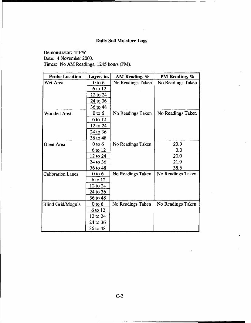
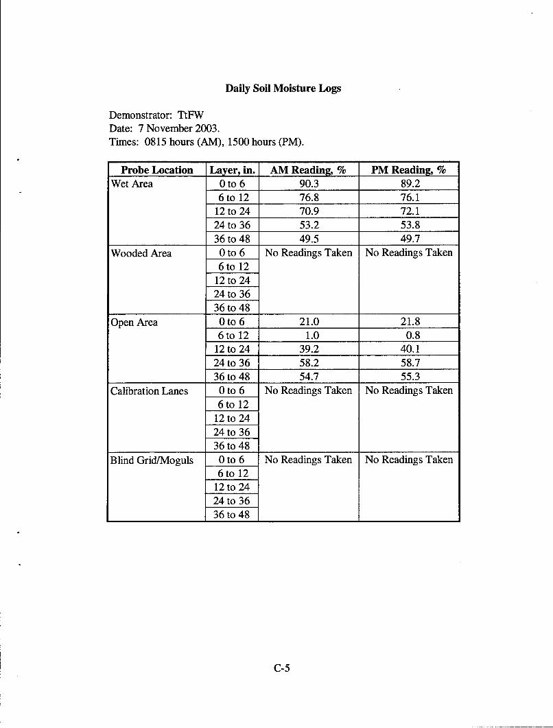
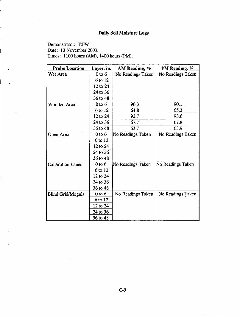
3.3.3 Soil Moisture

Five soil probes were placed at various locations of the site to capture soil moisturedata: wet, wooded, open, areas, calibration lanes, and blind grid/moguls. Measurements werecollected in percent moisture and were taken twice daily (morning and afternoon) from fivedifferent soil layers (0 to 6 in., 6 to 12 in., 12 to 24 in., 24 to 36 in., and 36 to 48 in.) from eachprobe. Soil moisture logs are included in Appendix C.

13

3.4 FIELD ACTIVITIES

3.4.1 Setup/Mobilization

These activities included initial mobilization and daily equipment preparation and breakdown. The three-person crew took 4 hours and 15 minutes to perform the initial setup andmobilization. No daily equipment preparation took place in the Blind Grid while end of dayequipment break down lasted 22 minutes on 3 November 2003.

3.4.2 Calibration

TtFW spent 1 hour and 37 minutes collecting data in the calibration lanes. Two othercalibration activities occurred in the Blind Grid using a metal to calibrate the RTS. Theseactivities totaled 6 minutes of site usage time.

3.4.3 Downtime Occasions

Occasions of downtime are grouped into five categories: equipment/data checks orequipment maintenance, equipment failure and repair, weather, Demonstration Site issues, orbreaks/lunch. All downtime is included for the purposes of calculating labor costs (section 5)except for downtime due to Demonstration Site issues. Demonstration Site issues, while noted inthe Daily Log, are considered nonchargeable downtime for the purposes of calculating laborcosts and are not discussed. Breaks and lunches are not discussed either.

3.4.3.1 Equipment/data checks, maintenance. Equipment/data checks and maintenanceactivities accounted for no site usage time in the blind grid. These activities included changingout batteries and routine data checks to ensure data were being properly recorded/collected.

3.4.3.2 Equipment failure or repair. No equipment failures occurred while surveying in theblind grid.

3.4.3.3 Weather. No delays occurred due to weather.

3.4.4 Data Collection

The demonstrator spent 1-hour collecting data in the blind grid. This time excludesbreak/lunches and downtimes described in section 3.4.3.

3.4.5 Demobilization

The demobilization time for the RTS took 2 hours and 35 minutes. On 13 November 2003,TtFW field crew packed up all equipment and permanently left the site.

3.5 PROCESSING TIME

TtFW submitted the raw data from demonstration activities before leaving the site on thelast day of the survey. The scoring submission data were also provided within the required 30-day timeframe.

14

3.6 DEMONSTRATOR'S FIELD PERSONNEL

Tim Deignan: Project GeophysicistMike McGuire: Geophysicist

3.7 DEMONSTRATOR'S FIELD SURVEYING METHOD

TtFW started surveying the blind grid in the northeast portion and surveyed in an east/westdirection. One lane was surveyed and then the demonstrator returned to the beginning of thenext lane (example: IA, lB, IC then 2A, 2B, 2C) until completion.

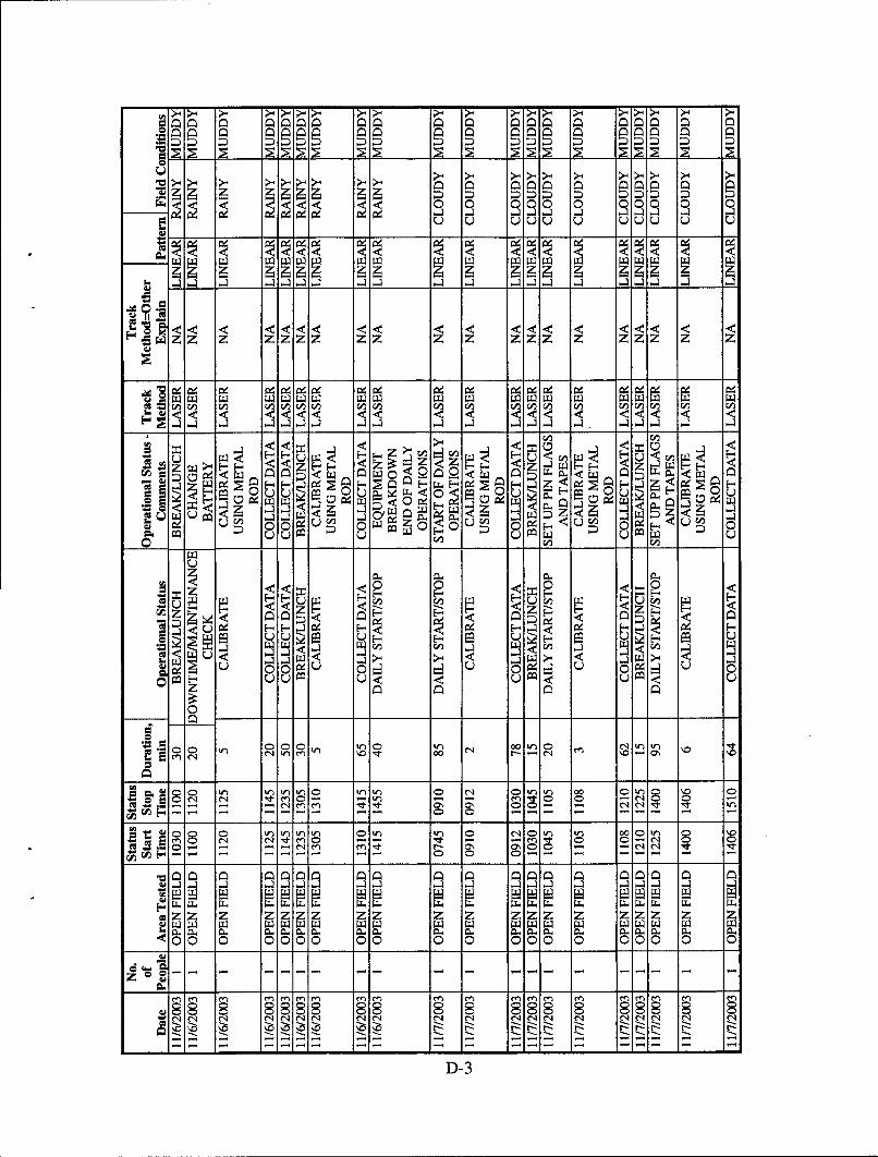
3.8 SUMMARY OF DAILY LOGS

Daily logs capture all field activities during this demonstration and are located in Appendix D.Activities pertinent to this specific demonstration are indicated in highlighted text.

No significant events occurred during the survey of the blind grid. The saturation of theblind grid was a minor distraction for TtFW.

15(Page 16 Blank)

SECTION 4. TECHNICAL PERFORMANCE RESULTS

4.1 ROC CURVES USING ALL ORDNANCE CATEGORIES

Figure 2 shows the probability of detection for the response stage (Pdr') and thediscrimination stage (Pdisc ) versus their respective probability of false positive. Figure 3 showsboth probabilities plotted against their respective probability of background alarm. Both figuresuse horizontal lines to illustrate the performance of the demonstrator at two demonstrator-specifiedpoints: at the system noise level for the response stage, representing the point below whichtargets are not considered detectable, and at the demonstrator's recommended threshold level forthe discrimination stage, defining the subset of targets the demonstrator would recommenddigging based on discrimination. Note that all points have been rounded to protect the groundtruth.

Noise LevelThreshold

------------ - , ...... . Response-------- -------- -- - Discriminaion

0I: ... .. .. .

0.2 0.4 0.6 0.8

Prob of False Positive

Figure 2. EM61 MKII blind grid probability of detection for response and discrimination stagesversus their respective probability of false positive over all ordnance categoriescombined.

17

NoisLevelThreshold

---- ------- ............................-------------- -........ .....R e s p o n s eo Discrimination

-- ---------

0 02 0.4 06 08 1Prob of Background Alarm

Figure 3. EM61 MKII blind grid probability of detection for response and discrimination stagesversus their respective probability of background alarm over all ordnance categoriescombined.

4.2 ROC CURVES USING ORDNANCE LARGER THAN 20-MM

Figure 4 shows the probability of detection for the response stage (Pdres) and thediscrimination stage (Pddisc) versus their respective probability of false positive when only targetslarger than 20-mm are scored. Figure 5 shows both probabilities plotted against their respectiveprobability of background alarm. Both figures use horizontal lines to illustrate the performanceof the demonstrator at two demonstrator-specified points: at the system noise level for theresponse stage, representing the point below which targets are not considered detectable, and atthe demonstrator's recommended threshold level for the discrimination stage, defining the subsetof targets the demonstrator would recommend digging based on discrimination. Note that allpoints have been rounded to protect the ground truth.

18

[. isLevelj-Threshold

2, . Response

o--[ Discrimination

.....-------- ..... .-- ----.-- --

CD r

0.2 0.4 0 0.8

Prob of False Positive

Figure 4. EM61 MKII blind grid probability of detection for response and discrimination stagesversus their respective probability of false positive for all ordnance larger than 20-mm.

ThresholdCq ..... Response

---- --- - ----- --- -- --- --- ---T -- --- --- -- Discriminationj

- - --

0

oc ..... . .

0 0.2 0.4 0.6 0.8 1

Prob of Background Alarm

Figure 5. EM61 MKII blind grid probability of detection for response and discrimination stagesversus their respective probabilities of background alarm for all ordnance larger than20-mm.

19

4.3 PERFORMANCE SUMMARIES

Results for the Blind Grid test, broken out by size, depth and nonstandard ordnance, arepresented in Table 6. (For cost results, see section 5.) Results by size and depth include bothstandard and nonstandard ordnance. The results by size show how well the demonstrator did atdetecting/discriminating ordnance of a certain caliber range. (See app A for size definitions.) Theresults are relative to the number of ordnances emplaced. Depth is measured from the closestpoint of anomaly to the ground surface.

The RESPONSE STAGE results are derived from the list of anomalies above thedemonstrator-provided noise level. The results for the DISCRIMINATION STAGE are derivedfrom the demonstrator's recommended threshold for optimizing UXO field cleanup byminimizing false digs and maximizing ordnance recovery. The lower 90-percent confidencelimit on probability of detection and probability of false positive was calculated assuming thatthe number of detections and false positives are binomially distributed random variables. Allresults in Table 5 have been rounded to protect the ground truth. However, lower confidencelimits were calculated using actual results.

TABLE 5. SUMMARY OF BLIND GRID RESULTS FOR EM61 MKII

I By Size By Depth, mMetric Overall Standard Nonstandard I Small Medium Large < 0.3 10.3 to <1 >= 1

RESPONSE STAGEPd 0.95 0.95 0.95 0.95 0.95 1.00 1.00 0.95 0.80

Pd Low 90% Conf 0.91 0.90 0.84 0.88 0.84 0.79 0.94 0.87 0.58Pfp 0.85 - 0.85 0.80 1.00Pf, Low 90% Conf 0.77 - 0.74 0.71 0.63

Pba 0.10 -- - -

DISCRIMINATION STAGEPd 0.75 0.85 0.65 0.85 0.70 0.80 0.90 0.80 0.35

Pd Low 90% Conf 0.70 0.76 0.53 0.74 0.55 0.55 0.81 0.67 0.19Pf _ 0.65 - - - - - 0.60 0.65 1.00Pf Low 90% Conf 0.58 - 0.49 0.56 0.63

Pba 0.05

Response Stage Noise Level: 0.00.Recommended Discrimination Stage Threshold: 1.00.

Note: The response stage noise level and recommended discrimination stage threshold valuesare provided by the demonstrator.

20

4.4 EFFICIENCY, REJECTION RATES, AND TYPE CLASSIFICATION

Efficiency and rejection rates are calculated to quantify the discrimination ability atspecific points of interest on the ROC curve: (1) at the point where no decrease in Pd is suffered(i.e., the efficiency is by definition equal to one) and (2) at the operator selected threshold.These values are reported in Table 6.

TABLE 6. EFFICIENCY AND REJECTION RATES

False Positive Background AlarmEfficiency (E) Rejection Rate Rejection Rate

At Operating Point 0.81 0.22 0.44With No Loss of Pd 1.00 0.00 0.00

At the demonstrator's recommended setting, the ordnance items that were detected andcorrectly discriminated were further scored on whether their correct type could be identified(table 7). Correct type examples include "20-mm projectile, 105-mm HEAT Projectile, and2.75-inch Rocket". A list of the standard type declaration required for each ordnance item wasprovided to demonstrators prior to testing. For example, the standard type for the three exampleitems are 20mmP, 105H, and 2.75in, respectively.

TABLE 7. CORRECT TYPE CLASSIFICATIONOF TARGETS CORRECTLY

DISCRIMINATEDAS UXO

Size % CorrectSmall 31.4Medium 38.1Large 37.5Overall 34.4

4.5 LOCATION ACCURACY

The mean location error and standard deviations appear in Table 8. These calculations arebased on average missed depth for ordnance correctly identified in the discrimination stage.Depths are measured from the closest point of the ordnance to the surface. For the Blind Grid,only depth errors are calculated, since (x, y) positions are known to be the centers of each gridsquare.

21

TABLE 8. MEAN LOCATION ERROR ANDSTANDARD DEVIATION

Mean, m Standard Deviation, mDepth -0.10 0.35

22

SECTION 5. ON-SITE LABOR COSTS

A standardized estimate for labor costs associated with this effort was calculated asfollows: the first person at the test site was designated "supervisor", the second person wasdesignated "data analyst", and the third and following personnel were considered "field support".Standardized hourly labor rates were charged by title: supervisor at $95.00/hour, data analyst at$57.00/hour, and field support at $28.50/hour.

Government representatives monitored on-site activity. All on-site activities weregrouped into one of ten categories: initial setup/mobilization, daily setup/stop, calibration,collecting data, downtime due to break/lunch, downtime due to equipment failure, downtime dueto equipment/data checks or maintenance, downtime due to weather, downtime due todemonstration site issue, or demobilization. See Appendix D for the daily activity logs. Seesection 3.4 for a summary of field activities.

The standardized cost estimate associated with the labor needed to perform the fieldactivities is presented in Table 9. Note that calibration time includes time spent in theCalibration Lanes as well as field calibrations. "Site survey time" includes daily setup/stop time,collecting data, breaks/lunch, downtime due to equipment/data checks or maintenance, downtimedue to failure, and downtime due to weather.

TABLE 9. ON-SITE LABOR COSTS

No. People Hourly Wage Hours [ CostINITIAL SETUP

Supervisor 1 $95.00 4.25 $403.75Data Analyst 1 57.00 4.25 242.25Field Support 1 28.50 4.25 121.13

Subtotal 1 $767.13CALIBRATION


Subtotal 1 $310.46SITE SURVEY


Subtotal $247.29

See notes at end of table.

23

TABLE 9 (CONT'D)

No. People Hourly Wage Hours CostDEMOBILIZATION


Subtotal $465.69Total ..... _$1,790.57

Notes: Calibration time includes time spent in the Calibration Lanes as well as calibrationbefore each data run.

Site Survey time includes daily setup/stop time, collecting data, breaks/lunch, downtimedue to system maintenance, failure, and weather.

24

SECTION 6. COMPARISON OF RESULTS TO DATE

No comparisons to date.

25(Page 26 Blank)

SECTION 7. APPENDIXES

APPENDIX A. TERMS AND DEFINITIONS

GENERAL DEFINITIONS

Anomaly: Location of a system response deemed to warrant further investigation by thedemonstrator for consideration as an emplaced ordnance item.

Detection: An anomaly location that is within Rhalo of an emplaced ordnance item.

Emplaced Ordnance: An ordnance item buried by the government at a specified location in thetest site.

Emplaced Clutter: A clutter item (i.e., non-ordnance item) buried by the government at aspecified location in the test site.

Rhalo: A pre-determined radius about the periphery of an emplaced item (clutter or ordnance)within which a location identified by the demonstrator as being of interest is considered to be aresponse from that item. For the purpose of this program, a circular halo 0.5 meters in radiuswill be placed around the center of the object for all clutter and ordnance items less than0.6 meters in length. When ordnance items are longer than 0.6 meters, the halo becomes anellipse where the minor axis remains 1 meter and the major axis is equal to the projected lengthof the ordnance onto the ground plane plus 1 meter.

Small Ordnance: Caliber of ordnance less than or equal to 40 mm (includes 20-mm projectile,40-mm projectile, submunitions BLU-26, BLU-63, and M42).

Medium Ordnance: Caliber of ordnance greater than 40 mm and less than or equal to 81 mm(includes 57-mm projectile, 60-mm mortar, 2.75-inch Rocket, MK1 18 Rockeye, 81-mm mortar).

Large Ordnance: Caliber of ordnance greater than 81 mm (includes 105-mm HEAT, 105-mmprojectile, 155-mm projectile, 500-lb bomb).

Shallow: Items buried less than 0.3 meter below ground surface.

Medium: Items buried greater than or equal to 0.3 meter and less than 1 meter below groundsurface.

Deep: Items buried greater than or equal to 1 meter below ground surface.

Response Stage Noise Level: The level that represents the point below which anomalies are notconsidered detectable. Demonstrators are required to provide the recommended noise level forthe Blind Grid test area.

A-1

Discrimination Stage Threshold: The demonstrator selects the threshold level that they believeprovides optimum performance of the system by retaining all detectable ordnance and rejectingthe maximum amount of clutter. This level defines the subset of anomalies the demonstratorwould recommend digging based on discrimination.

Binomially Distributed Random Variable: A random variable of the type which has only twopossible outcomes, say success and failure, is repeated for n independent trials with theprobability p of success and the probability 1-p of failure being the same for each trial. Thenumber of successes x observed in the n trials is an estimate of p and is considered to be abinomially distributed random variable.

RESPONSE AND DISCRIMINATION STAGE DATA

The scoring of the demonstrator's performance is conducted in two stages. These twostages are termed the RESPONSE STAGE and DISCRIMINATION STAGE. For both stages,the probability of detection (Pd) and the false alarms are reported as receiver-operatingcharacteristic (ROC) curves. False alarms are divided into those anomalies that correspond toemplaced clutter items, measuring the probability of false positive (Pfp) and those that do notcorrespond to any known item, termed background alarms.

The RESPONSE STAGE scoring evaluates the ability of the system to detect emplacedtargets without regard to ability to discriminate ordnance from other anomalies. For theRESPONSE STAGE, the demonstrator provides the scoring committee with the location andsignal strength of all anomalies that the demonstrator has deemed sufficient to warrant furtherinvestigation and/or processing as potential emplaced ordnance items. This list is generated withminimal processing (e.g., this list will include all signals above the system noise threshold). Assuch, it represents the most inclusive list of anomalies.

The DISCRIMINATION STAGE evaluates the demonstrator's ability to correctly identifyordnance as such, and to reject clutter. For the same locations as in the RESPONSE STAGEanomaly list, the DISCRIMINATION STAGE list contains the output of the algorithms appliedin the discrimination-stage processing. This list is prioritized based on the demonstrator'sdetermination that an anomaly location is likely to contain ordnance. Thus, higher output valuesare indicative of higher confidence that an ordnance item is present at the specified location. Forelectronic signal processing, priority ranking is based on algorithm output. For other systems,priority ranking is based on human judgment. The demonstrator also selects the threshold thatthe demonstrator believes will provide "optimum" system performance (i.e., that retains all thedetected ordnance and rejects the maximum amount of clutter).

Note: The two lists provided by the demonstrator contain identical numbers of potential targetlocations. They differ only in the priority ranking of the declarations.

A-2

RESPONSE STAGE DEFINITIONS

Response Stage Probability of Detection (pdres): Pdr' = (No. of response-stage detections)/(No. of emplaced ordnance in the test site).

Response Stage False Positive (fprs): An anomaly location that is within Rhalo of an emplacedclutter item.

Response Stage Probability of False Positive (pfpres): pfreS = (No. of response-stage falsepositives)/(No. of emplaced clutter items).

Response Stage Background Alarm: An anomaly in a blind grid cell that contains neitheremplaced ordnance nor an emplaced clutter item. An anomaly location in the open field orscenarios that is outside Rhalo of any emplaced ordnance or emplaced clutter item.

Response Stage Probability of Background Alarm (Pbares): Blind Grid only: Pbares = (No. ofresponse-stage background alarms)/(No. of empty grid locations).

Response Stage Background Alarm Rate (BARres): Open Field only: BARres = (No. ofresponse-stage background alarms)/(arbitrary constant).

Note that the quantities Pdres, pf PbareS, and BARres are functions of tr s, the thresholdapplied to the response-stage signal strength. These quantities can, therefore, be written asPdres(tres), PfpreS(tres), Pbares(tres), and BARrs(tres).

DISCRIMINATION STAGE DEFINITIONS

Discrimination: The application of a signal processing algorithm or human judgment toresponse-stage data that discriminates ordnance from clutter. Discrimination should identifyanomalies that the demonstrator has high confidence correspond to ordnance, as well as thosethat the demonstrator has high confidence correspond to nonordnance or background returns.The former should be ranked with highest priority and the latter with lowest.

Discrimination Stage Probability of Detection (Pddisc): Pddisc = (No. of discrimination-stagedetections)/(No. of emplaced ordnance in the test site).

Discrimination Stage False Positive (fpdis): An anomaly location that is within Rhalo of an

emplaced clutter item.

Discrimination Stage Probability of False Positive (pfpdic): pfpdisc = (No. of discrimination stagefalse positives)/(No. of emplaced clutter items).

Discrimination Stage Background Alarm: An anomaly in a blind grid cell that contains neitheremplaced ordnance nor an emplaced clutter item. An anomaly location in the open field orscenarios that is outside Rhalo of any emplaced ordnance or emplaced clutter item.

A-3

Discrimination Stage Probability of Background Alarm (PbadiSc): Pbadis = (No. of discrimination-stage background alarms)/(No. of empty grid locations).

Discrimination Stage Background Alarm Rate (BARdiSC): BARdisc = (No. of discrimination-stagebackground alarms)/(arbitrary constant).

Note that the quantities Pddisc, pfpdisc, Pbadisc, and BAR disc are functions of tdisc, the thresholdapplied to the discrimination-stage signal strength. These quantities can, therefore, be written as

Pd dSc(tdisc), pfpdiSc(tdisc), PbadiSc(tdisc), and BARdiSc(tdisc).

RECEIVER-OPERATING CHARACERISTIC (ROC) CURVES

ROC curves at both the response and discrimination stages can be constructed based on theabove definitions. The ROC curves plot the relationship between Pd versus Pfp and Pd versusBAR or Pba as the threshold applied to the signal strength is varied from its minimum (tmin) to itsmaximum (tmax) value.' Figure A-I shows how Pd versus Pfp and Pd versus BAR are combinedinto ROC curves. Note that the "res" and "disc" superscripts have been suppressed from all thevariables for clarity.

max max s

t Ii t tin

Pd train < t < t". Pd / tmi n < t < tmtax -

tm tmax

0 - 0

0 Pfp max 0 BAR max

Figure A-1. ROC curves for open-field testing. Each curve applies to both the response anddiscrimination stages.

'Strictly speaking, ROC curves plot the Pd versus Pba over a predetermined and fixed number ofdetection opportunities (some of the opportunities are located over ordnance and others arelocated over clutter or blank spots). In an open field scenario, each system suppresses its signalstrength reports until some bare-minimum signal response is received by the system.Consequently, the open field ROC curves do not have information from low signal-outputlocations, and, furthermore, different contractors report their signals over a different set oflocations on the ground. These ROC curves are thus not true to the strict definition of ROCcurves as defined in textbooks on detection theory. Note, however, that the ROC curvesobtained in the Blind Grid test sites are true ROC curves.

A-4

METRICS TO CHARACTERIZE THE DISCRIMINATION STAGE

The demonstrator is also scored on efficiency and rejection ratio, which measure theeffectiveness of the discrimination stage processing. The goal of discrimination is to retain thegreatest number of ordnance detections from the anomaly list, while rejecting the maximumnumber of anomalies arising from nonordnance items. The efficiency measures the amount ofdetected ordnance retained by the discrimination, while the rejection ratio measures the fractionof false alarms rejected. Both measures are defined relative to the entire response list, i.e., themaximum ordnance detectable by the sensor and its accompanying false positive rate orbackground alarm rate.

Efficiency (E): E = pddi c(tdisc)/pdres(tin res): measures (at a threshold of interest), the degreeto which the maximum theoretical detection performance of the sensor system (as determined bythe response stage trin) is preserved after application of discrimination techniques. Efficiency isa number between 0 and 1. An efficiency of 1 implies that all of the ordnance initially detected

discin the response stage was retained at the specified threshold in the discrimination stage, t

False Positive Rejection Rate (Rfp): Rfp = 1 - [Pfpdisc(tdisc)/pfpres(tminres)]: measures (at athreshold of interest), the degree to which the sensor system's false positive performance isimproved over the maximum false positive performance (as determined by the response stagetin). The rejection rate is a number between 0 and 1. A rejection rate of 1 implies that allemplaced clutter initially detected in the response stage were correctly rejected at the specifiedthreshold in the discrimination stage.

Background Alarm Rejection Rate (Rba):

Blind Grid: Rba = 1- [Pbadisc(tdisc)/Pbares(tminres)]

Open Field: Rba = 1 - [BARd'sc(tdi)/BARres(tnnres)])

Measures the degree to which the discrimination stage correctly rejects background alarmsinitially detected in the response stage. The rejection rate is a number between 0 and 1. Arejection rate of 1 implies that all background alarms initially detected in the response stage wererejected at the specified threshold in the discrimination stage.

CHI-SQUARE COMPARISON EXPLANATION:

The Chi-square test for differences in probabilities (or 2 x 2 contingency table) is used toanalyze two samples drawn from two different populations to see if both populations have thesame or different proportions of elements in a certain category. More specifically, two randomsamples are drawn, one from each population, to test the null hypothesis that the probability ofevent A (some specified event) is the same for both populations (ref 4).

A 2 x 2 contingency table is used in the Standardized UXO Technology DemonstrationSite Program to determine if there is reason to believe that the proportion of ordnance correctlydetected/discriminated by demonstrator X's system is significantly degraded by the more

A-5

challenging terrain feature introduced. The test statistic of the 2 x 2 contingency table is theChi-square distribution with one degree of freedom. Since an association between the morechallenging terrain feature and relatively degraded performance is sought, a one-sided test isperformed. A significance level of 0.05 is chosen which sets a critical decision limit of2.71 from the Chi-square distribution with one degree of freedom. It is a critical decision limitbecause if the test statistic calculated from the data exceeds this value, the two proportions testedwill be considered significantly different. If the test statistic calculated from the data is less thanthis value, the two proportions tested will be considered not significantly different.

An exception must be applied when either a 0 or 100 percent success rate occurs in thesample data. The Chi-square test cannot be used in these instances. Instead, Fischer's test isused and the critical decision limit for one-sided tests is the chosen significance level, which inthis case is 0.05. With Fischer's test, if the test statistic is less than the critical value, theproportions are considered to be significantly different.

Standardized UXO Technology Demonstration Site examples, where blind grid results arecompared to those from the open field and open field results are compared to those from one ofthe scenarios, follow. It should be noted that a significant result does not prove a cause andeffect relationship exists between the two populations of interest; however, it does serve as a toolto indicate that one data set has experienced a degradation in system performance at a largeenough level than can be accounted for merely by chance or random variation. Note also that aresult that is not significant indicates that there is not enough evidence to declare that anythingmore than chance or random variation within the same population is at work between the twodata sets being compared.

Demonstrator X achieves the following overall results after surveying each of the threeprogressively more difficult areas using the same system (results indicate the number ofordnance detected divided by the number of ordnance emplaced):

Blind Grid Open Field MogulsPd' s 100/100 = 1.0 8/10 = .80 20/33 = .61Pddisc 80/100 = 0.80 6/10 = .60 8/33 = .24

Pdrs: BLIND GRID versus OPEN FIELD. Using the example data above to compareprobabilities of detection in the response stage, all 100 ordnance out of 100 emplaced ordnanceitems were detected in the blind grid while 8 ordnance out of 10 emplaced were detected in theopen field. Fischer's test must be used since a 100 percent success rate occurs in the data.Fischer's test uses the four input values to calculate a test statistic of 0.0075 that is comparedagainst the critical value of 0.05. Since the test statistic is less than the critical value, the smallerresponse stage detection rate (0.80) is considered to be significantly less at the 0.05 level ofsignificance. While a significant result does not prove a cause and effect relationship existsbetween the change in survey area and degradation in performance, it does indicate that thedetection ability of demonstrator X's system seems to have been degraded in the open fieldrelative to results from the blind grid using the same system.

A-6

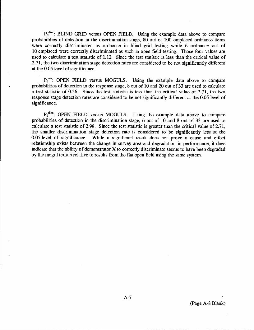
Pd:disc BLIND GRID versus OPEN FIELD. Using the example data above to compareprobabilities of detection in the discrimination stage, 80 out of 100 emplaced ordnance itemswere correctly discriminated as ordnance in blind grid testing while 6 ordnance out of10 emplaced were correctly discriminated as such in open field testing. Those four values areused to calculate a test statistic of 1.12. Since the test statistic is less than the critical value of2.71, the two discrimination stage detection rates are considered to be not significantly differentat the 0.05 level of significance.

Pds: OPEN FIELD versus MOGULS. Using the example data above to compareprobabilities of detection in the response stage, 8 out of 10 and 20 out of 33 are used to calculatea test statistic of 0.56. Since the test statistic is less than the critical value of 2.71, the tworesponse stage detection rates are considered to be not significantly different at the 0.05 level ofsignificance.

Pddisc: OPEN FIELD versus MOGULS. Using the example data above to compareprobabilities of detection in the discrimination stage, 6 out of 10 and 8 out of 33 are used tocalculate a test statistic of 2.98. Since the test statistic is greater than the critical value of 2.71,the smaller discrimination stage detection rate is considered to be significantly less at the0.05 level of significance. While a significant result does not prove a cause and effectrelationship exists between the change in survey area and degradation in performance, it doesindicate that the ability of demonstrator X to correctly discriminate seems to have been degradedby the mogul terrain relative to results from the flat open field using the same system.

A-7(Page A-8 Blank)

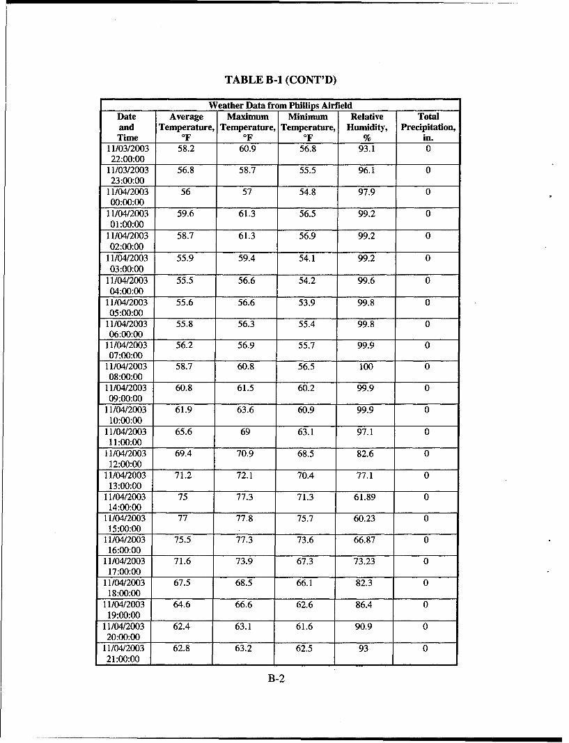
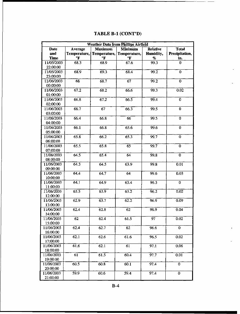
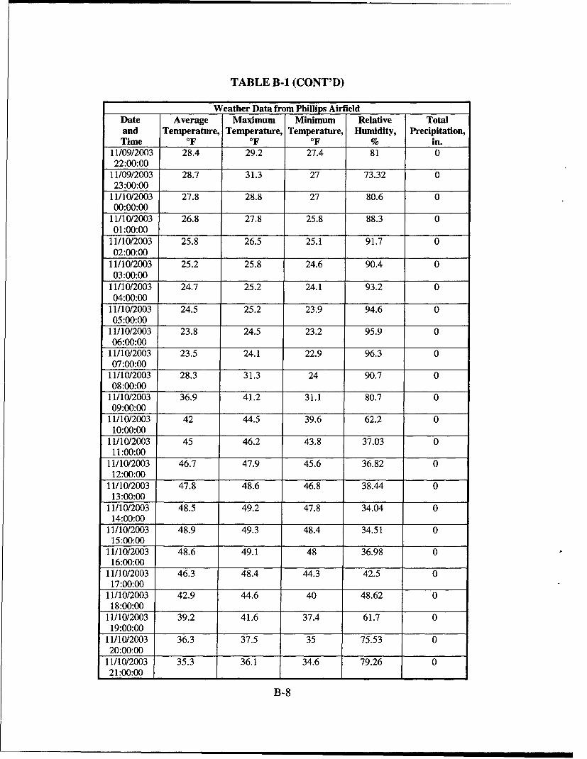
APPENDIX B. DAILY WEATHER LOGS

TABLE B-1. WEATHER LOG

Weather Data from Phillips AirfieldDate Average Maximum Minimum Relative Totaland Temperature, Temperature, Temperature, Humidity, Precipitation,Time OFF F % in.

11/03/2003 56.7 57.9 55.8 98.7 000:00:00

11/03/2003 55.4 56 54.8 98.9 001:00:00

11/03/2003 54.3 55 53.6 99.1 002:00:00

11/03/2003 54.4 55.1 53.5 99.3 003:00:00

11/03/2003 53.7 54.7 52.4 99.3 004:00:00

11/03/2003 52.7 53.4 51.7 99.4 005:00:00

11/03/2003 52.6 53.3 51.8 99.5 006:00:00

11/03/2003 51.7 52.4 51.1 99.5 007:00:00

11/03/2003 52.7 54.8 51.5 99.7 008:00:00

11/03/2003 58.4 61.4 54.6 99.8 009:00:00

11/03/2003 63.8 67.5 60.9 94.1 010:00:00

11/03/2003 70.6 73.3 67.2 74.86 011:00:00

11/03/2003 74.8 75.8 73 62.95 012:00:00

11/03/2003 76.4 77.8 75.3 55.86 .013:00:00

11/03/2003 77.9 78.7 76.9 51.94 014:00:00

11/03/2003 78 78.4 77.6 51.56 015:00:00

11/03/2003 77.1 78.2 76 53.6 016:00:00

11/03/2003 74.3 76.5 71.7 58.49 017:00:00

11/03/2003 69.7 72 67 66.53 018:00:00

11/03/2003 65.4 67.3 62.3 76.28 019:00:00

11/03/2003 63.2 65.3 60.4 81.9 020:00:00

11/03/2003 62 63.6 60.4 85.5 021:00:00

B-1

TABLE B-i (CONT'D)

_________Weather Data fro Phillips AirfieldDate Average Maximum Minimum Relative Totaland Temperature, Temperature, Temperature, Humidity, Precipitation,Time OF F OF____% in.

11/03/2003 58.2 60.9 56.8 93.1 022:00:00

11/03/2003 56.8 58.7 55.5 96.1 023:00:00 1____________ ______

11/04/2003 56 57 54.8 97.9 000:00:00__ _ __ _ _

11/04/2003 59.6 61.3 56.5 99.2 001:00:00 1

11/04/2003 58.7 61.3 56.9 99.2 002:00:00

11/04/2003 55.9 59.4 54.1 99.2 003:00:00 __ ___

11/04/2003 55.5 56.6 54.2 99.6 004:00:00

11/04/2003 55.6 56.6 53.9 99.8 005 :00:00

11/04/2003 55.8 56.3 55.4 99.8 006 :00:00 _________________ _____

11/04/2003 56.2 56.9 55.7 99.9 007 :00:00 __ ____

11/04/2003 58.7 60.8 56.5 100 008:00:00 __ ___

11/04/2003 60.8 61.5 60.2 99.9 009:00:00 ______ _____

11/04/2003 61.9 63.6 60.9 99.9 010:00:00 ____________ _____ _____

11/04/2003 65.6 69 63.1 97.1 011:00:00_ _ _

11/04/2003 69.4 70.9 68.5 82.6 012:00:00 __________________

11/04/2003 71.2 72.1 70.4 77.1 013:00:00 _______

11/04/2003 75 77.3 71.3 61.89 014:00:00 ______

11/0/2003 77 77.8 75.7 60.23 015:00:00 ______________

11/04/2003 75.5 77.3 73.6 66.87 016 :00: 00 _____ _ ____

11/04/2003 71.6 73.9 67.3 73.23 017:00:00

11/042003 67.5 68.5 66.1 82.3 018:00:00 ___________________ ______

11/04/2003 64.6 66.6 62.6 86.4 019:00:00__________ ___

11/04/2003 62.4 63.1 61.6 90.9 020:00:00 ____________

11/042003 62.8 63.2 62.5 93 021:00:00 ______ ________________________

B-2

TABLE B-1 (CONT'D)

Weather Data from Phillips AirfieldDate Average Maximum Minimum Relative Totaland Temperature, Temperature, Temperature, Humidity, Precipitation,Time OFF F % in.

11/04/2003 62.3 63 61.5 96.4 022:00:00

11/04/2003 61.6 62 61.2 98.7 023:00:00

11/05/2003 61.1 61.5 60.7 99.2 000:00:00

11/05/2003 60.9 61.4 60.4 99.5 001:00:00

11/05/2003 61 61.4 60.6 99.6 002:00:00

11/05/2003 61.3 61.6 60.9 99.6 003:00:00

11/05/2003 61.1 61.5 60.7 99.7 004:00:00

11/05/2003 60.7 61.3 60.3 99.7 005:00:00

11/05/2003 60.6 60.9 60.2 99.8 006:00:00

11/05/2003 60.6 61.2 60.1 99.8 007:00:00

11/05/2003 60.9 61.3 60.6 99.8 008:00:00

11/05/2003 61.4 62 60.8 99.9 009:00:00

11/05/2003 62.2 63 61.4 99.9 010:00:00

11/05/2003 62.9 64 62 99.9 011:00:00

11/05/2003 64.2 65.6 63.4 99.9 012:00:00

11/05/2003 67.7 69.6 65.5 99.8 013:00:00

11/05/2003 70.5 71.3 68.6 98.8 014:00:00

11/05/2003 72 73.3 70.9 93.2 015:00:00

11/05/2003 71.4 73.7 70 90.7 016:00:00

11/05/2003 69.8 70.2 69.1 94.1 0.0217:00:00

11/05/2003 69.5 70.4 68.7 96.9 0.118:00:00

11/05/2003 69.2 70 68.7 97.9 0.0519:00:00

11/05/2003 68.7 69.2 68.2 98.6 0.0320:00:00

11/05/2003 68 68.6 67.2 99 021:00:00 1 1 1 _ _1_ _

B-3

TABLE B-I (CONT'D)

Weather Data from Phillips AirfieldDate Average Maximum Minimum Relative Totaland Temperature, Temperature, Temperature, Humidity, Precipitation,Time OF OF OF % in.

11/05/2003 68.3 68.9 67.6 99.3 022:00:00

11/05/2003 68.9 69.3 68.4 99.2 023:00:00

11/06/2003 68 68.7 67 99.2 000:00:00

11/06/2003 67.2 68.2 66.6 99.3 0.0201:00:00

11/06/2003 66.8 67.2 66.5 99.4 002:00:00

11/06/2003 66.7 67 66.3 99.5 003:00:00

11/06/2003 66.4 66.8 66 99.5 004:00:00

11/06/2003 66.1 66.8 65.6 99.6 005:00:00

11/06/2003 65.8 66.2 65.3 99.7 006:00:00

11/06/2003 65.5 65.8 65 99.7 007:00:00

11/06/2003 64.5 65.4 64 99.8 008:00:00

'11/06/2003 64.3 64.5 63.9 99.8 0.0109:00:00

11/06/2003 64.4 64.7 64 99.6 0.0310:00:00

11/06/2003 64.1 64.9 63.4 96.3 011:00:00

11/06/2003 63.5 63.9 63.2 96.2 0.0212:00:00

11/06/2003 62.9 63.7 62.2 96.9 0.0913:00:00

11/06/2003 62.4 62.8 62 96.9 0.0414:00:00

11/06/2003 62 62.4 61.5 97 0.0215:00:00

11/06/2003 62.4 62.7 62 96.6 016:00:00

11/06/2003 62.1 62.6 61.6 96.5 0.0217:00:00

11/06/2003 61.6 62.1 61 97.1 0.0618:00:00

11/06/2003 61 61.5 60.4 97.7 0.0119:00:00

11/06/2003 60.5 60.8 60.1 97.4 020:00:00

11/06/2003 59.9 60.6 59.4 97.4 021:00:00

B-4

TABLE B-1 (CONT'D)


11/06/2003 59.6 60 59.4 97.8 022:00:00

11/06/2003 59.4 60 58.9 97.9 023:00:00

11/07/2003 58.8 59.4 58.3 98.3 0.0200:00:00

11/07/2003 58.6 58.9 58.3 98.5 0.0101:00:00

11/07/2003 58.6 58.9 58.2 98.1 002:00:00

11/07/2003 58.3 58.8 57.9 97.9 003:00:00

11/07/2003 57.8 58.4 57.2 96.2 004:00:00

11/07/2003 57.4 57.7 57 95.8 005:00:00

11/07/2003 57 57.6 56.4 95.3 006:00:00

11/07/2003 56.3 56.9 55.7 88.2 007:00:00 1

11/07/2003 55.5 56 55.1 86.5 008:00:00

11/07/2003 55.3 55.8 55 82.8 009:00:00

11/07/2003 55.6 56.3 55 79.4 010:00:00

11/07/2003 55.8 57.7 54.7 76.8 011:00:00

11/07/2003 57.3 58.4 55.5 68.16 012:00:00

11/07/2003 58.6 60.2 57.6 56.83 013:00:00

11/07/2003 59.5 60.9 58.5 48.84 014:00:00

11/07/2003 60.1 61 59 44.86 015:00:00

11/07/2003 58.3 59.7 57.5 46.07 016:00:00

11/07/2003 56.6 57.8 54.3 53.22 017:00:00

11/07/2003 52.1 54.6 49.7 67.05 018:00:00

11/07/2003 49.8 52 48 73.88 019:00:00

11/07/2003 49.4 50.2 48.2 75.81 020:00:00

11/07/2003 51 52.5 48.9 64.81 021:00:00 1 1 1

B-5

TABLE B-1 (CONT'D)


11/07/2003 52.2 53 51.3 53.84 022:00:00

11/07/2003 51.5 53 49.2 48.53 023:00:00

11/08/2003 49.5 50.2 48.6 56.35 000:00:00

11/08/2003 50.3 50.8 49.6 50.08 001:00:00

11/08/2003 50 50.9 48.6 37.29 002:00:00

11/08/2003 47.6 49.1 46.7 38.99 003:00:00

11/08/2003 45.8 47 44.5 42.26 004:00:00

11/08/2003 42.6 44.7 41 52.06 005:00:00

11/08/2003 41.7 42.4 40.5 54.25 006:00:00

11/08/2003 40.2 41.8 38.6 60.22 007:00:00

11/08/2003 42.2 44.4 39.8 58.77 008:00:00

11/08/2003 46 47.7 44.1 50.81 009:00:00

11/08/2003 47.6 48.4 47 46.72 010:00:00

11/08/2003 48.7 49.6 47.9 44.69 011:00:00

11/08/2003 48.8 50.4 46.9 46.64 012:00:00

11/08/2003 47.6 48.7 46.5 47.39 013:00:00

11/08/2003 46.8 47.6 46 44.97 014:00:00

11/08/2003 45.9 47.3 45 41.94 015:00:00

11/08/2003 44.9 45.6 43.8 37.58 016:00:00

11/08/2003 42.9 44.3 41 38.61 017:00:00

11/08/2003 40.5 41.3 39.4 41.07 018:00:00

11/08/2003 39.3 39.9 38.8 43 019:00:00

11/08/2003 38.9 39.3 38.4 42.13 020:00:00

11/08/2003 38.4 38.8 37.9 40.23 021:00:00

B-6

TABLE B-1 (CONT'D)


11/08/2003 38.1 38.5 37.6 37.94 022:00:00

11/08/2003 37.8 38.2 37.3 37.31 023:00:00

11/09/2003 37.4 37.8 36.7 37.18 000:00:00

11/09/2003 36.4 37.3 35.2 37.59 001:00:00

11/09/2003 34.7 35.5 34 41.03 002:00:00

11/09/2003 33.6 34.4 32.6 43.24 003:00:00

11/09/2003 32.2 33.1 31.4 46.99 004:00:00

11/09/2003 31.2 32 30.7 50.54 005:00:00

11/09/2003 30.4 31.1 29.6 53.81 006:00:00

11/09/2003 29.8 30.2 29.4 56.49 007:00:00

11/09/2003 31.7 33.8 29.6 54.91 008:00:00

11/09/2003 35.1 36.7 33.4 46.47 009:00:00

11/09/2003 37.9 39 36.4 42.15 010:00:00

11/09/2003 39.5 40.5 38.5 39.16 011:00:00

11/09/2003 41.2 42.4 39.9 34.3 012:00:00

11/09/2003 43.3 45.3 41.7 30.22 013:00:00

11/09/2003 44.6 45.8 43.1 26.02 014:00:00

11/09/2003 45.6 46.7 44.4 23.61 015:00:00

11/09/2003 44.2 45.6 43.5 24.34 016:00:00

11/09/2003 42 43.7 40.7 24.2 017:00:00

11/09/2003 38.2 41 36.3 29.51 018:00:00

11/09/2003 34.4 36.6 32.8 40.71 019:00:00

11/09/2003 31.2 33.3 29.5 64.51 020:00:00

11/09/2003 29.5 30.1 28.6 74.18 021:00:00 1 t I I _

B-7

TABLE B-1 (CONT'D)


11/09/2003 28.4 29.2 27.4 81 022:00:00

11/09/2003 28.7 31.3 27 73.32 023:00:00

11/10/2003 27.8 28.8 27 80.6 000:00:00

11/10/2003 26.8 27.8 25.8 88.3 001:00:00

11/10/2003 25.8 26.5 25.1 91.7 002:00:00

11/10/2003 25.2 25.8 24.6 90.4 003:00:00

11/10/2003 24.7 25.2 24.1 93.2 004:00:00

11/10/2003 24.5 25.2 23.9 94.6 005:00:00

11/10/2003 23.8 24.5 23.2 95.9 006:00:00 E

11/10/2003 23.5 24.1 22.9 96.3 007:00:00

11/10/2003 28.3 31.3 24 90.7 008:00:00

11/10/2003 36.9 41.2 31.1 80.7 009:00:00

11/10/2003 42 44.5 39.6 62.2 010:00:00

11/10/2003 45 46.2 43.8 37.03 011:00:00

11/10/2003 46.7 47.9 45.6 36.82 012:00:00

11/10/2003 47.8 48.6 46.8 38.44 013:00:00

11/10/2003 48.5 49.2 47.8 34.04 014:00:00

11/10/2003 48.9 49.3 48.4 34.51 015:00:00

11/10/2003 48.6 49.1 48 36.98 016:00:00

11/10/2003 46.3 48.4 44.3 42.5 017:00:00

11/10/2003 42.9 44.6 40 48.62 018:00:00

11/10/2003 39.2 41.6 37.4 61.7 019:00:00

11/10/2003 36.3 37.5 35 75.53 020:00:00

11/10/2003 35.3 36.1 34.6 79.26 021:00:00

B-8

L

TABLE B-i (CONT'D)


11/10/2003 34.6 35.4 33.7 84.7 022:00:00

11/10/2003 34.4 35.9 33.3 85.7 023:00:00

11/11/2003 35.1 36.1 33.8 89 000:00:00

11/11/2003 34.3 35.1 33.3 92.2 001:00:00

11/11/2003 33.6 34.6 32.8 95.3 002:00:00

11/11/2003 34 36.8 32.9 93.4 003:00:00

11/11/2003 33.6 34.9 32.7 96.9 004:00:00

11/11/2003 34.5 35.9 32.7 97.3 005:00:00

11/11/2003 34 35.5 32.8 98.1 006:00:00

11/11/2003 34.4 37.5 32.6 99.1 007:00:00

11/11/2003 39.8 45 36.7 93.3 008:00:00

11/11/2003 47.5 49.5 44.6 81.1 009:00:00

11/11/2003 51.7 53.2 49.3 80.2 010:00:00

11/11/2003 53.3 54.6 52.2 80.1 011:00:00

11/11/2003 54.8 55.4 54.2 80.4 012:00:00 1

11/11/2003 55.9 56.5 55.1 77.78 013:00:00

11/11/2003 56.2 57.7 54.8 78.04 014:00:00

11/11/2003 57.3 58.1 56.7 72.77 015:00:00

11/11/2003 56.8 57.2 56.5 71.21 016:00:00

11/11/2003 56.6 57.1 55.9 74.34 017:00:00

11/11/2003 56.5 57.1 55.8 76.62 018:00:00

11/11/2003 55.8 56.4 55.3 80.4 019:00:00

11/11/2003 54.8 55.8 53.6 84.9 020:00:00

11/11/2003 53.6 54.3 53 92.1 021:00:00

B-9

TABLE B-I (CONT'D)


11/11/2003 53.1 53.6 52.6 94.4 022:00:00

11/11/2003 53.1 53.9 52.1 92 023:00:00

11/12/2003 52.6 52.9 52.2 94.8 000:00:00

11/12/2003 52.5 52.9 52.2 95.6 0.0301:00:00

11/12/2003 52.6 52.9 52.2 97.7 0.0402:00:00

11/12/2003 52.7 53 52.3 98.3 0.0703:00:00

11/12/2003 52.7 52.9 52.2 98.7 0.0204:00:00

11/12/2003 52.9 53.2 52.4 99.1 0.205:00:00

11/12/2003 52.9 53.2 52.6 99.3 0.1306:00:00

11/12/2003 52.8 53 52.4 99.4 0.0707:00:00

11/12/2003 52.8 53.2 52.6 99.5 0.0908:00:00

11/12/2003 53.1 53.4 52.7 99.6 0.0109:00:00

11/12/2003 53.6 54.2 52.9 99.5 010:00:00

11/12/2003 54.6 55.2 53.6 98.7 011:00:00

11/12/2003 54.8 55.5 54.1 97.5 012:00:00 1

11/12/2003 55.8 56.3 55 95.1 013:00:00

11/12/2003 56 56.5 55.8 94.9 014:00:00

11/12/2003 55.8 56.2 55.4 96.8 015:00:00

11/12/2003 55.9 56.5 55.4 97.1 016:00:00

11/12/2003 55.8 56.6 55.2 96.7 017:00:00

11/12/2003 55.4 55.7 55.1 98.2 018:00:00

11/12/2003 55.7 56 55.3 98.2 019:00:00

11/12/2003 55.7 56 55.3 98 020:00:00

11/12/2003 55.5 55.8 55.2 98.1 021:00:00

B-10

TABLE B-1 (CONT'D)


11/12/2003 56.2 57.7 55.2 98.5 022:00:00

11/12/2003 58.8 60 57.5 97.7 0.0223:00:00

11/13/2003 60.3 60.8 59.5 97.5 000:00:00

11/13/2003 60.9 61.4 60.4 97.5 001:00:00

11/13/2003 60.6 61 60.1 97.4 002:00:00

11/13/2003 60.3 60.8 60 97.2 003:00:00

11/13/2003 59.9 61.8 58.8 92.4 004:00:00

11/13/2003 61 62 59.6 54.85 005:00:00

11/13/2003 57.9 60.1 55.5 39 006:00:00

11/13/2003 52.6 55.7 49.9 43.56 007:00:00

11/13/2003 49.5 50.2 48.4 50.59 008:00:00

11/13/2003 49.4 50.8 48.4 45.75 009:00:00

11/13/2003 48.8 49.5 47.7 46.31 010:00:00

11/13/2003 48.9 49.5 48.1 43.07 011:00:00

11/13/2003 48.5 49.6 47.6 32.95 012:00:00

11/13/2003 49.2 50.4 47.4 29.37 013:00:00

11/13/2003 47.4 49.7 45.7 35.59 014:00:00

11/13/2003 46.3 47.2 45 36.44 015:00:00

11/13/2003 44.6 45.4 43.7 39.58 016:00:00

11/13/2003 43.3 44.1 42.2 43.6 017:00:00

11/13/2003 42.3 43 41.7 44.66 018:00:00

11/13/2003 41.8 42.5 41.2 46.95 019:00:00

11/13/2003 41.7 42.1 41.2 46.6 020:00:00

11/13/2003 41.6 42.2 41.3 43.61 021:00:00 1 1 1 1 _1

B-11

TABLE B-i (CONT'D)

__________ Weather Data frm Phillips Airfield______Date Average Maximum Minimum Relative Totaland Temperature, Temperature, Temperature, Humidity, Precipitation,Time OF OF OF____% in.

11/13/2003 41.8 42.2 41.5 40.58 022:00:00 _____ __________

11/13/2003 41.6 42.1 412 40.44 023:00:00 ___7___ I____

B-12

APPENDIX C. SOIL MOISTURE

Daily Soil Moisture Logs

Demonstrator: TtFWDate: 3 November 2003.Times: No AM Readings, 1300 hours (PM).

Probe Location Layer, in. AM Reading, % PM Reading, %Wet Area 0 to 6 No Readings Taken No Readings Taken

6to 1212 to 2424to 3636 to 48

Wooded Area 0 to 6 No Readings Taken No Readings Taken6to 12

12 to 2424 to 3636 to 48

Open Area 0 to 6 No Readings Taken No Readings Taken6to 12

12 to 2424 to 3636 to 48

Calibration Lanes 0 to 6 No Readings Taken 38.76 to 12 36.9

12 to 24 8.424 to 36 5.136 to 48 5.3

Blind Grid/Moguls 0 to 6 No Readings Taken 2.56 to 12 15.2

12 to 24 37.124 to 36 36.836 to 48 38.4

C-1


Demonstrator: TtFWDate: 4 November 2003.Times: No AM Readings, 1245 hours (PM).


6to 1212 to 2424 to 3636 to 48


12 to 2424 to 3636 to 48

Open Area 0 to 6 No Readings Taken 23.96 to 12 3.0

12 to 24 20.024 to 36 21.936 to 48 38.6

Calibration Lanes 0 to 6 No Readings Taken No Readings Taken6to 12

12 to 2424 to 3636 to 48

Blind Grid/Moguls 0 to 6 No Readings Taken No Readings Taken6to 12

12 to 2424 to 3636 to 48 _ ]

C-2


Demonstrator: TtFWDate: 5 November 2003.Times: 1130 hours (AM), 1400 hours (PM).


6 to 1212 to 2424 to 36

_____ _____ _____ 36 to 48 _ _ _ _ _ _ _ _ _ _ _ _ _ _ _ _ _

Wooded Area 0 to 6 No Readings Taken No Readings Taken6 to 12

12 to 2424 to 3636 to 48

Open Area Oto 6 13.7 13.66 to 12 1.1 1.5

12 to24 16.0 15.824 to36 20.0 20.9

___________36 to 48 27.9 28.5

Calibration Lanes 0 to 6 11.1 No Readings Taken6to 12 37.7

12 to24 7.824 to36 4.536 to 48 4.6 _______

Blind Grid/Moguls 0 to 6 2.2 No Readings Taken6 to 12 14.5

12 to 24 36.424 to36 36.3

____________36 to48 38.1________

C-3



Probe Location Layer, in. AM Reading, % PM Reading, %Wet Area 0 to 6 88.3 89.7

6 to 12 77.3 77.712 to 24 69.3 69.924 to 36 52.1 52.836 to 48 49.1 49.2


12 to 2424 to 3636 to 48

Open Area 0 to 6 21.2 21.76 to 12 1.5 1.7

12 to 24 38.8 38.124 to 36 59.1 59.336 to 48 54.7 54.6


12 to 2424 to 3636 to 48


12 to 2424 to 3636 to 48

C-4




6 to 12 76.8 76.112 to 24 70.9 72.124 to 36 53.2 53.836 to 48 49.5 49.7


12 to 2424 to 3636 to 48

Open Area 0 to 6 21.0 21.86 to 12 1.0 0.8

12 to 24 39.2 40.124 to 36 58.2 58.736 to 48 54.7 55.3


12 to 2424 to 3636 to 48


12 to 2424 to 3636 to 48

C-5


Demonstrator: TtFWDate: 10 November 2003.Times: 0800 hours (AM), 13 10 hours (PM).


6 to 12 82.7 82.112 to 24 75.1 75.324 to36 55.1 55.5

__________36 to48 51.3 51.0

Wooded Area 0 to 6 No Readings Taken No Readings Taken6 to 12

12 to 2424 to 36

____ ___ ____ ___ 36 to 48

Open Area 0 to 6 20.4 20.26 to 12 2.6 3.0

12 to 24 17.3 16.924 to 36 17.2 16.9

___________36 to 48 34.3 34.1

Calibration Lanes 0 to 6 No Readings Taken No Readings Taken6 to 12

12 to 2424 to 36

____ ____ ____ ___ 36 to_48 _ _ _ _ _ _ _ _ _

Blind Grid/Moguls 0 to 6 No Readings Taken No Readings Taken6 to 12

12 to 2424 to 3636 to_48 _ _ _ _ _ _ _ _ _ ______ ___

C-6




6 to 12 82.2 82.712 to 24 74.5 73.924 to 36 54.4 55.236 to 48 50.6 51.3

Wooded Area 0 to 6 76 No Readings Taken6 to 12 65.6

12 to 24 92.724 to 36 65.136 to 48 57.5

Open Area 0 to 6 20.8 20.16 to 12 2.8 2.6

12 to 24 16.8 17.324 to 36 16.9 17.136 to 48 33.7 34.8


12 to 2424 to 3636 to 48

Blind Grid/Moguls 0 to 6 No Readings Taken 2.36 to 12 33.7

12 to 24 35.824 to 36 36.036 to 48 38.1

C-7


Demonstrator: TtFWDate: 12 November 2003.Times: 1000 hours (AM), No PM Readings.


6to 1212 to 2424 to 3636 to 48

Wooded Area 0 to 6 74.2 No Readings Taken6 to 12 78.5

12 to 24 91.224 to 36 64.836 to 48 58.0


12 to 2424 to 3636 to 48


12 to 2424 to 3636 to 48

Blind Grid/Moguls 0 to 6 2.4 No Readings Taken6 to 12 34.8

12 to 24 37.324 to 36 36.636 to 48 38.5

C-8




6to 1212 to 2424to 3636 to 48

Wooded Area 0 to 6 90.3 90.16 to 12 64.8 65.3

12 to 24 93.7 93.624 to 36 67.7 67.836 to 48 63.7 63.9


12 to 2424 to 3636 to 48


12 to 2424 to 3636 to 48


12 to 2424to 3636 to 48

C-9

APPENDIX D. DAILY ACTIVITY LOGS

U)) . . . 1 99 -

CIP __ __ __ _n En_ W n ( 0 w V 0

zg z z z z z z z z z z z z

c) )0 o nF- W

__ _ __ _ _ C). _ _ w U94 1: u 0404 9

u u u u

1:4 14 0

o u u U I U I lU m-

o< 0

S0 0 E- 0 -0u - 'u u

N0

W)0 F %c 0 0) W F) w.0 I'D) '0 ~ ' l Ccn C' C14 C') C') C') C') C') I ) W)0 -

' 0 W) 0 0 0 0 0 N M--F-

z~~~~ z0 Z E E

0 cU' C') C') U' C') C') C' C' C' C' C'u ' ' ' '

------------------------------------ m >

D-1

PC ~ ~ -

"a z z

0 >~>~ ~ z

W000 000 E-0 0000 E- 0 000 w0 in 00 000 u0

En ~ -z z- Z0 00- Z Z

<z

2 0H

UU0 0

00

C) 00 coo 0 -CV 0

0 0 D C )oo w 0 k n c

00 C0 00 0 '

00 00 000 CD Cn0 0 W)0' 0cqi 0I1 me ' v) 0 ) N0 ci m m- mne v)

N~c CAe m mn "t o 0 00 O\ C71 C-M )0 0 0 0 0

00~~~ ~~~~ 9 0 0 0 0 0n 0 n n

ZO en 'nc ze 'n dO 0 en zt 'e e

48 mn Mn n C ~ 0 0\ 0C

o n n en -) -) m -

D-2

JS0 0 00

0 00 0 0 0

u U L)Uu

ElaC z z z z z z

0

4. C/ In (A c V)) f/) CA (A (A W c) C6 _ W _ V ___ C

W) En'

~~U~U~aU) 00 U a 0 zUrU U

o~C Cd) "FCd

U

u 0 U 0 o C U C U upU 0/0 0 0 0

00

u nn

ci uCJ -'n 0 w ~U)V F -- -- n

00 tnnnn 0 Wn c 0') n C1 n 't0

- rci 0 0)e

'~00 0 00 00 0 00000

Ww~ w w w00 o0 toc 0 0 000 0 000 0 0

4.'-

0 + ---

D-3

-D D

Sz z z zz z z z~ z z z z z z z

<< .1 << 5

< w t nn

oi g =~ 5w ,-W > ___ __ C.o

C) < .

IX

0ow0 0 0 - - -

0 0 0 00 00 0 0 0

E- E- 2D=4

0 0 00

F W V) < W) Q<- ; <W 4 ' 2

00) 0 0 0000 000 000 p 000 0 :0 000W0 z~

lo Z z1 0 0z

F. 0 000 0

E U -o0 o0 00 o~ 00 00 .J0

0< < w u< w U u u u L

0 0

En W) CA InW

or- 0IU-IO 0 I~

0 0) IO 0 ) 0 ) M tn 00 WIn 0 0Iw c') N ~ In tn c r- C14 O0 0- -It

n -) -n -n ) -0 0)

0 C14 "~ cqm

0n 0n 00 00 00 c0 0 000 n enC40

nM 0 ' ~ ~ ' l C ll C~ l C~ l C~

PC ~C< .- - . -

In I nn\ \ C) DO O ~ O ~ww 0 -z -z z - -z -z z - z z

0 0 0 0 0 o D-5

00 00 0 00 0

~~~0~~ 0 00E00 0 0 0 0

Z Z ZZZ ZZ ~zZz zz z z z zz

~0CCo /)CC C - 4 CCCC/ 0 C/ CC C C Z CC C CC

sUl 8 CZ 04 E

-3 U u W

00 0 0u U > u CU)0 0U u

0 0

00

<Z <Z 0 0 0

En ~ 0 Z ~ < ~ 0 ~ ~n 0' n

O\~~~~ u\'C <~~'- 't- ~ ~ n i -oC'n~ ~*C ~ ~ e cc- n n z- ' n

En~ 0) CI

~~~o~ 0 00 0 ~ Q

en cn eq ..

NZ Z CtI M 0-- tn 0 0 D e ) 0V 0 0---------------------------------------------------------------- m- W

eq N n n d-ItIt I W t 0 0D(N6O

I-S

Zz ZzZ zzzz Zzz z z z ZzzZ ZZ

u U,

0 2

U- u uc )uU U C4C) u L u_

zr~ < ~~~ Z 0 0

0 z 0 a zno

00 mb 0

~u0E 0

0 00 00 000 W 000t 0k 0 4 0<< <

*t0 00 00 00 0 000 0 0 0) k

0 0 000 - -- - -tt

pD-

m o ~zz~ z z

cn En F- 9 w 0 wU, O <- z# < - -w '' z<-'F- >

0 0

U U~ U, U,4,U~F- w

OF- I F-

0T 0000

SI R_ !2 ___ CM

00 00 tn~00

00 00\ Cl 0- O 00 O

0~4 00 - - 0 0 0 - 0 0

0 00 0 0

eq cq el

D-8

E oz z z z z00

~II.< < < <Z

< < < z

g0 D o

r~ <

C,, _ _

cc Oo00 '

Z I) rCI) CI

Wa D-9

(PgeD 1 lak

APPENDIX E. REFERENCES

1. Standardized UXO Technology Demonstration Site Handbook, DTC ProjectNo. 8-CO-160-000-473, Report No. ATC-8349, March 2002.

2. Aberdeen Proving Ground Soil Survey Report, October 1998.

3. Data Summary, UXO Standardized Test Site: APG Soils Description, May 2002.

4. Practical Nonparametric Statistics, W.J. Conover, John Wiley & Sons, 1980, pages144 through 151.

E-1(Page E-2 Blank)

APPENDIX F. ABBREVIATIONS

ACE = Army Corps of EngineersAEC = US Army Environmental CenterAPG = Aberdeen Proving GroundATC = US Army Aberdeen Test CenterCST = Arc Secon ConstellationEQT = Army Environmental Quality Technology ProgramERDC = US Army Corps of Engineers Engineering Research and Development CenterESTCP = Environmental Security Technology Certification ProgramDGPS = differential Global Positioning SystemGPO = geophysical prove-outHERO = Hazards of Electromagnetic Radiation to OrdnanceHz = hertzJPG = Jefferson Proving GroundPCMIA = Personal Computer Memory Card International AssociationPOC = point of contactQA = quality assuranceQC = quality controlROC = receiver-operating characteristicRTS = Robotic Total StationSERDP = Strategic Environmental Research and Development ProgramTtFW = Tetra Tech Foster WheelerUXO = unexploded ordnanceVDS = verification of detection systemYPG = U.S. Army Yuma Proving Ground

F-1(Page F-2 Blank)

APPENDIX G. DISTRIBUTION LIST

DTC Project No. 8-CO-160-UXO-021

No. ofAddressee Copies

CommanderU.S. Army Environmental CenterATTN: SFIM-AEC-PCT 2Aberdeen Proving Ground, MD 21010-5401

Tetra Tech Foster Wheeler, Inc.143 Union Blvd., Suite 1010 1Lakewood, CO 80212

CommanderU.S. Army Aberdeen Test CenterATTN: CSTE-DTC-AT-SL-F (Mr. Larry Overbay) 2

(Library) 1CSTE-DTC-AT-TC-C (Ms. Barbara Gillich) 1

(Ms. Carolyn Berger) 1CSTE-DTC-AT-CS-RM 1

Aberdeen Proving Ground, MD 21005-5059

Technical DirectorU.S.Army Test and Evaluation Command

ATTN: CSTE-TD (Mr. Brian Barr) 14501 Ford AvenueAlexandria, VA 22302-1458

Defense Technical Information Center 28725 John J. Kingman Road, STE 0944Fort Belvoir, VA 22060-6218

Secondary distribution is controlled by Commander, U.S. Army Environmental Center,ATTN: SFIM-AEC-PCT.

G-1(Page G-2 Blank)

Date post:	17-Mar-2020
Category:	Documents
Upload:	others
View:	1 times
Download:	0 times

,,j5SERDP - DTICThe public reporing. burden for this collection of information is estimated to...

Documents