SENSING AND DETECTION OF A PRIMARY RADIO SIGNAL IN A COGNITIVE RADIO ENVIRONMENT USING MODULATION IDENTIFICATION TECHNIQUE Jide Julius Popoola A thesis submitted to the Faculty of Engineering and the Built Environment, University of the Witwatersrand, Johannesburg, in fulfilment of the requirements for the degree of Doctor of Philosophy. Johannesburg, 2012
Transcript
SENSING AND DETECTION OF A PRIMARY RADIO SIGNAL IN A COGNITIVE RADIO ENVIRONMENT USING MODULATION
IDENTIFICATION TECHNIQUE
Jide Julius Popoola
A thesis submitted to the Faculty of Engineering and the Built Environment, University of the Witwatersrand, Johannesburg, in fulfilment of the requirements for the degree of Doctor of Philosophy. Johannesburg, 2012
ii
DECLARATION
I declare that this thesis is my own unaided work. It is being submitted to the degree of
Doctor of Philosophy to the University of the Witwatersrand, Johannesburg. It has not
been submitted before for any degree or examination in any University.
………………………………………………………………………. (Signature of the Candidate) ……9th……… day of …… May…………… 2012
iii
ABSTRACT
In today’s society, the need for the right information at the right time and the right place
as well as increased number of high bandwidth wireless multimedia services and the
explosive proliferation of smart phone and tablet devices has led to increase in demand
for and use of radio spectrum, which is the primary enabler of wireless communications.
With this increase, the principal engineering challenge in wireless communications
domain is now on how to effectively manage the radio spectrum to ensure its
sustainability for future emerging wireless devices, since virtually all usable radio
frequencies for wireless communications have been licensed to commercial users and
government agencies.
Traditionally, the approach to radio spectrum management has been based on a fixed
allocation policy, whereby licenses are issued to users or operators for the usage of
frequency bands. With a license, operators have the exclusive right to use the allocated
frequency bands for assigned services on a long-term basis. However, over the last ten
years, this strict allocation policy has been subjected to a lot of criticism because of its
observed contribution to radio spectrum scarcity and underutilization.
In mitigating these negative effects of the current radio spectrum management policy, one
of the suggested measures is to open up the licensed frequency bands to unlicensed users
on a non-interference basis to licensed users. In this new spectrum access system, an
unlicensed or secondary user can opportunistically operate in unused licensed spectrum
bands without interfering with the licensed or primary user, thereby reducing radio
spectrum scarcity and at the same time increasing the efficiency of the radio spectrum
utilization.
In achieving this objective, there is a need to develop a radio engine that can sense its
environment to determine the presence of primary users. Cognitive radio is seen as the
enabling technology for opportunistic spectrum sharing. It is a radio with the capability to
sense and understand its environment, and proactively alter its operational mode as
needed to avoid interference with a primary user. To ensure interference-free use to the
iv
primary user, spectrum sensing and detection has been observed as a key functionality of
cognitive radio.
However, there is currently no single sensing method that can reliably sense and detect
all forms of primary radios’ signals in a cognitive radio environment. Therefore, in order
to achieve this goal, this thesis addresses the problem of accurate and reliable sensing and
detecting of a primary radio signal in a cognitive radio environment. The principal
research issue addressed is the possibility of sensing and detecting all forms of primary
radio signals in a cognitive radio environment. This objective was achieved by
developing an adaptive cognitive radio engine that can automatically recognize different
forms of modulation schemes in a cognitive radio environment.
The thesis pictures spectrum sensing as the combination of signal detection and
modulation classification, and uses the term Automatic Modulation Classification (AMC)
to denote this combined process. The hypothesis behind this detection method is that,
since all transmitters using the radio spectrum make use of one modulation scheme or
another, the ability to automatically recognize modulation schemes is sufficient to
confirm the presence of a primary user signal while the opposite confirms absence of a
primary user signal.
The research work methodology was divided into two stages. The first stage involves the
development of an automatic modulation recognition (AMR) or AMC using an Artificial
Neural Network (ANN). The second stage involves the development of the Cognitive
Radio Engine (CRE), which has the developed AMR as its core component. The
developed CRE was extensively evaluated to determine its performance. The overall
numerical results obtained from the developed CRE’s evaluation shows that the
developed CRE can reliably and accurately detect all the modulation schemes considered
without bias towards a particular Signal-to-Noise Ratio (SNR) value, as well as any
modulation scheme. The research work also revealed that single spectrum sensing and
detection method can only be achieved when a general feature common to all radio
signals is employed in its development rather than using features that are limited to
certain signal types.
v
DEDICATION
To my treasured and lovely wife,
Misitura Abiola Popoola
vi
ACKNOWLEDGEMENTS Out of many that I am indebted to, I wish to express my profound appreciation to the following people:
� The Almighty God, my Lord and Saviour, Jesus Christ and my comforter, the Holy Spirit, who inspires and endorses the actualization of my dreams;
� My parents, Mr. and Mrs. Elijah Adeboye Popoola, who instilled in me a desire
for formal education, despite their lack thereof. I will surely be forever grateful for the foundation they laid for me in life;
� My supervisor, Prof. Rex van Olst, deserves my acknowledgement for his
guidance, supervision, commitment, encouragement and rare thoroughness during this research period. I thank him for editing this thesis and providing direction. Thank you for the opportunities you gave me to prove my ability;
� My faithful wife, Abiola, for holding fort while I was away from home in pursuit
of this degree, and my children, Victory, Peace and Faith, for living their babyhood in absence of their father. You all deserve an honorary degree;
� Prof. Ian Jandrell and Prof. Barry Dwolatkzy are also acknowledged for their
encouragement and sustained interest in my success;
� Dr. A. Sengur of Firat University, Technical Education Faculty, Turkey, for his invaluable input on conceptualization of the feature extraction keys methodology;
� Dr. James Adewumi, Dr. Sola Ilemobade and Dr. Peter Olubambi including their
respective families for their assistance and encouragement;
� My colleagues in the School of Electrical and Information Engineering, University of the Witwatersrand, Johannesburg: Ryan van de Bergh, David Vannucci, Sade Dahunsi, Bolanle Abe, Mehroze Abdullah and Doron Horwitz; these represent many others I cannot mention as a result of space constraints. I recognize your immense contributions;
� Centre for Telecommunications Access and Services (CeTAS) for financial
assistance;
� The University of the Witwatersrand Financial Aids and Scholarships for financial assistance;
� Reverend Charity Odeyemi, Pastor Gbadebo Popoola and Pastor Gbenga Ojo as
well as their families and all members of Dominion Family Church for their constant encouragement; and
vii
� Lastly, all my friends and colleagues from the Federal University of Technology, Akure, Nigeria, who are too numerous to mention here.
viii
LIST OF PUBLICATIONS
Journal Publications Jide Julius Popoola and Rex van Olst (2011). A novel modulation sensing method: Remedy for uncertainty around the practical use of cognitive radio technology. IEEE Vehicular Technology Magazine, vol. 6, no. 3, pp. 60-69, September 2011. Jide Julius Popoola and Rex van Olst (2011). Automatic recognition of analog modulated signals using artificial neural networks. Journal of Computer Technology and Applications, vol. 2, no. 1, pp. 29-35, January 2011. Jide Julius Popoola and Rex van Olst. Performance evaluation of Spectrum sensing implementation using an automatic modulation classification detection method with universal software radio peripheral. Submitted to “An International Journal on Performance Evaluation” Elsevier Publisher. Jide Julius Popoola and Rex van Olst. A survey on dynamic spectrum access via cognitive radio: taxonomy, requirement, and benefits. Submitted to “Telecommunications Policy” Elsevier Publisher. Conference Publications Jide Julius Popoola and Rex van Olst (2011): “Automatic classification of combined analog and digital modulation schemes using feedforward neural network,” in Proceedings of 10th IEEE AFRICON 2011, The Falls Resort and Convention Centre, Livingstone, Zambia, 13 – 15 September 2011. Jide Julius Popoola and Rex van Olst (2011): “Application of neural network for sensing primary radio signals in a cognitive radio environment,” in Proceedings of 10th IEEE AFRICON 2011, The Falls Resort and Convention Centre, Livingstone, Zambia, 13 – 15 September 2011. Jide Julius Popoola and Rex van Olst (2011): “Cooperative sensing reliability improvement algorithm for primary radio signal detection in cognitive radio environment,” in Proceedings of Southern Africa Telecommunication Networks and Applications Conference 2011 (SATNAC 2011), East London, South Africa, pp. 131-136, 4 – 7 September 2011. Jide Julius Popoola and Rex van Olst (2011): “Novel modulation sensing method as a remedy for uncertainty around the practical use of cognitive radio technology,” in Proceedings of 26th Wireless World Research Forum 2011 (WWRF 2011), Doha, Qatar, 11 - 13 April 2011.
ix
Jide Julius Popoola and Rex van Olst (2010): “Dynamic spectrum access as an alternative radio spectrum regulation system,” in Proceedings of 2nd Region 8 IEEE Conference on History of Telecommunications (HISTELCON 2010), Madrid, Spain, 3 - 5 November 2010. Jide Julius Popoola and Rex Van Olst (2009): “Application of online modulation recognition in detection of analog modulated primary radio signals in cognitive radio environment,” in Proceedings of South African Institute of Computer Scientists and Information Technologists 2009 (SAICSIT 2009) Masters and Doctoral Symposium, Riversides Hotel and Conference Centre, VanderbijlPark, Vaal Rivers, South Africa, 10 – 14 October 2009. Jide Julius Popoola and Rex van Olst (2009): “Detection of primary radio signals in cognitive radio environment,” in Proceedings of Southern Africa Telecommunication Networks and Applications Conference 2009 (SATNAC 2009), Royal Swazi Spa, Swaziland, pp. 469-470, 30 August – 2 September 2009.
x
TABLE OF CONTENTS
SENSING AND DETECTION OF A PRIMARY RADIO SIGNAL IN A COGNITIVE RADIO ENVIRONMENT USING MODULATION IDENTIFICATION TECHNIQUE i DECLARATION ................................................................................................................ ii ABSTRACT ....................................................................................................................... iii ACKNOWLEDGEMENTS ............................................................................................... vi LIST OF PUBLICATIONS ............................................................................................. viii TABLE OF CONTENTS .................................................................................................... x LIST OF FIGURES ......................................................................................................... xvi LIST OF TABLES ........................................................................................................... xix LIST OF TABLES ........................................................................................................... xix LIST OF ABBREVIATIONS .......................................................................................... xxi CHAPTER 1 ....................................................................................................................... 1 1.0 INTRODUCTION AND BACKGROUND OF THE STUDY .............................. 1
1.1 Introduction ......................................................................................................... 1 1.2 Radio Spectrum Management ............................................................................. 4 1.3 The Need for Flexibility in Spectrum Management ........................................... 6 1.4 Enabler of Flexibility Spectrum Management .................................................... 7 1.5 Problem Statement/Motivation ......................................................................... 11 1.6 Research Aim and Objectives ........................................................................... 12 1.7 The Relevance of this Research Work .............................................................. 12 1.8 The Thesis Outline ............................................................................................ 13
CHAPTER 2 ..................................................................................................................... 16 2.0 LITERATURE REVIEW ..................................................................................... 16
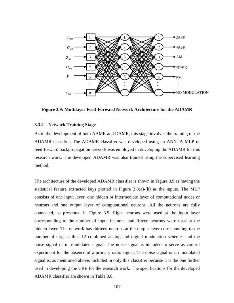
xi
2.1 Radio Evolution Technology ............................................................................ 16 2.2 Software Defined Radio .................................................................................... 17 2.3 Implementation of Software Defined Radio ..................................................... 19
2.3.1 GNU Radio ............................................................................................... 20 2.3.1.1 Gnu Radio Sources ....................................................................................... 21 2.3.1.2 Gnu Radio Sinks ........................................................................................ 21 2.3.1.3 Gnu Radio Flow Graphs ........................................................................... 21 2.3.1.4 Gnu Radio Schedulers............................................................................... 22 2.3.2 Universal Software Radio Peripheral........................................................ 22
2.4 Artificial Intelligence Techniques in Cognitive Radio ..................................... 23 2.5 Cognitive Engine .............................................................................................. 24 2.6 Area of Application of Cognitive Radio ........................................................... 26
2.6.1 Dynamic Exclusive Use Model ................................................................ 27 2.6.2 Open Sharing Model ................................................................................. 28 2.6.3 Hierarchical Access Model ....................................................................... 28 2.6.3.1 Spectrum Underlay ................................................................................... 28 2.6.3.2 Spectrum Overlay...................................................................................... 29
2.12.2.3 Reinforcement Learning............................................................................ 73 2.12.3 Transfer Function ...................................................................................... 74
4.1 Cooperative Sensing Time Algorithm Development ...................................... 115 4.2 Cooperative Spectrum Sensing Optimization ................................................. 119
4.2.1 Number of Cognitive Radios Collaborating ........................................... 120 4.2.2 Effect of Fine Frequency Sensing Resolution Selection ......................... 121
xiv
4.2.3 Impact of Effect of α value Selection ..................................................... 122 4.3 Comparative Analysis of the Developed Sensing Time Algorithm................ 123 4.4 Summary ......................................................................................................... 125
CHAPTER 5 ................................................................................................................... 126 5.0 DEVELOPMENT OF THE STUDY COGNITIVE RADIO ENGINE ............. 126
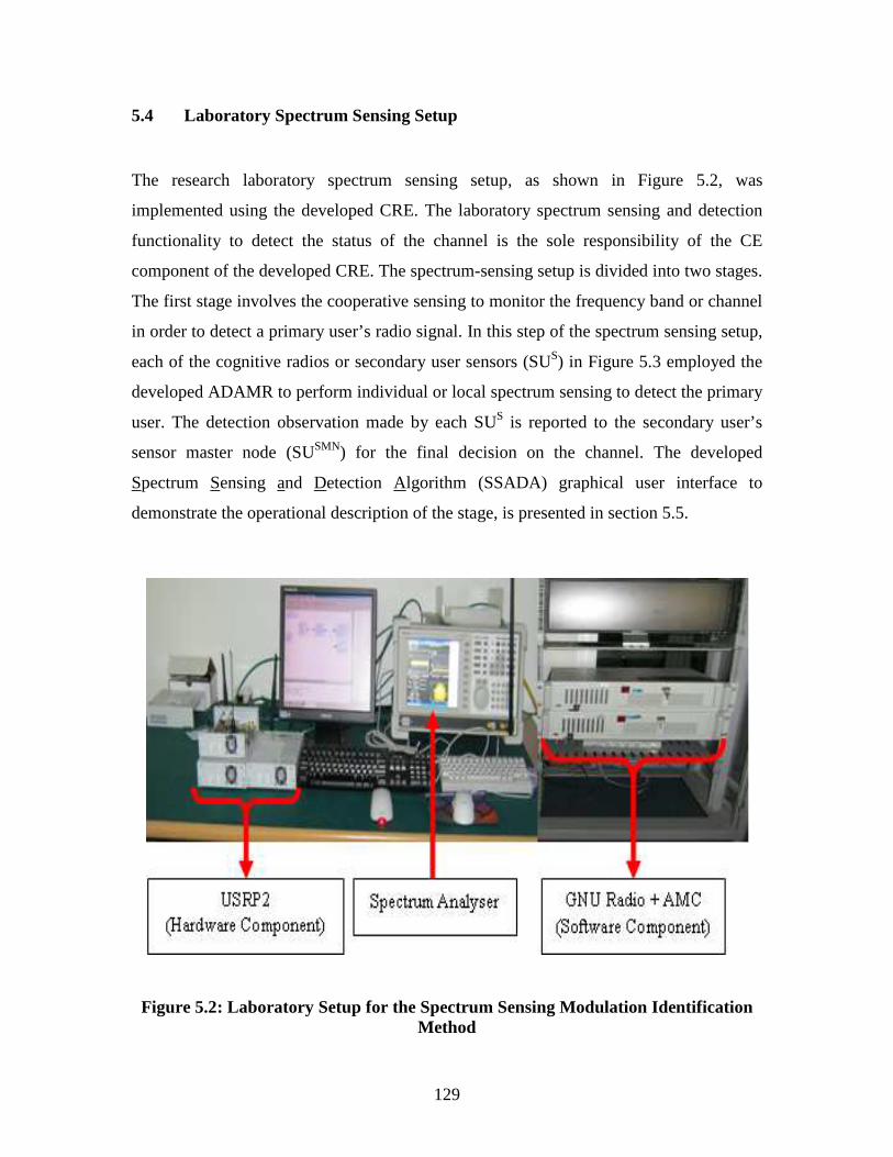
5.1 Cognitive Engine Development ...................................................................... 126 5.2 Software Defined Radio Development ........................................................... 128 5.3 Coupling of the Developed SDR and CE ....................................................... 128 5.4 Laboratory Spectrum Sensing Setup ............................................................... 129 5.5 Developed Spectrum Sensing and Detection Algorithm Description ............. 132 5.6 Summary ......................................................................................................... 139
CHAPTER 6 ................................................................................................................... 140 6.0 THE DEVELOPED COGNITIVE RADIO ENGINE EVALUATION ............. 140
6.1 Experimental Evaluation of the Developed Cognitive Radio Engine ............ 140
6.1.1 Detection States ...................................................................................... 140 6.1.2 Probability of Detection .......................................................................... 142 6.1.3 Detection Response Time ....................................................................... 145
CHAPTER 7 ................................................................................................................... 154 7.0 RESEARCH SUMMARY AND CONCLUSION.............................................. 154
xv
7.1 Thesis Summary.............................................................................................. 154 7.2 Conclusion and Recommendation .................................................................. 156 7.3 Future Work Recommendations ..................................................................... 158
APPENDIX A: M-FILE FOR THE THREE CLASSIFIERS ........................................ 176 APPENDIX B: GNU RADIO INSTALLATION AND USRP2 CONFIGURATION .. 189 APPENDIX C: USER MANUAL FOR SPECTRUM SENSING AND DETECTION ALGORITHM................................................................................................................. 195
xvi
LIST OF FIGURES Figure 1.1: Spectrum Utilization......................................................................................... 6
Figure 1.2: Relationship between Applications, Ownership and Spectrum ....................... 8
Figure 1.3: The Dissertation Outline Flowchart ............................................................... 15
Figure 2.1: The Evolution of Radio Technology .............................................................. 17
Figure 2.2: Software Defined Radio Communication System.......................................... 19
Figure 2.3: USRP Motherboard without Daughterboard .................................................. 20
Radio spectrum is a natural resource with some special characteristics (Hatfield, 1993).
The key characteristics of the radio spectrum are the propagation features and the amount
of information that signals can carry (Cave et al., 2006). In general, according to these
authors, signals sent using the higher frequencies reach shorter distances, but have a
higher information-carrying capacity. These physical characteristics of radio spectrum
limit the currently identified range of applications for which any particular frequency
band is suitable.
On the other hand, unlike most natural resources, such as oil, coal, iron or other mineral
resources, radio spectrum’s unique characteristics is that it is not consumed by use. This
means that the resource is infinitely renewable. Since it is renewable, radio spectrum
cannot be accumulated for later use but must be properly managed. These factors
therefore necessitate an efficient process for making radio spectrum available for
purposes which are useful to society (Cave et al., 2006).
1.2 Radio Spectrum Management
As a public resource, radio spectrum is being managed by governments to ensure that it is
shared equitably to promote the public interest, convenience, or necessity (Nunno, 2002).
It is being tightly regulated around the world by both the international and national
regulators. At international level, the International Telecommunication Union (ITU) is
managing spectrum. The International Telecommunication Union-Radiocommunication
(ITU-R) Sector maintains a table of frequency allocations which identifies spectrum
bands for about forty (40) categories of wireless services with the aim of avoiding
interference among those services. Once the broad categories are established, each
country may allocate spectrum for various services within its own borders in compliance
with ITU’s table of frequency allocations. The table divides the world into three regions.
Region 1 includes Africa and Europe, region 2 includes North and South America, and
region 3 includes Australia and Asia.
5
At the national level, the use of radio spectrum in most countries is currently being
managed by government agencies rather than by market forces. For instance, in the
United Kingdom, it is being regulated by the Office of Communications (Ofcom) while
the Federal Communications Commission (FCC) is responsible for radio spectrum
regulation in the United States. The Independent Communications Authority of South
Africa (ICASA), the Nigerian Communications Commission (NCC), the Ministry of
Communication Technology and Transport (MCTT), the Communications Commission
of Kenya (CCK) and the National Communications Authority (NCA) to mention but a
few, are responsible for radio spectrum regulation in South Africa, Nigeria, Tunisia,
Kenya and Ghana respectively. In most of these countries, the primary tool of spectrum
management by government is a licensing system. This involves spectrum being
apportioned into blocks for specific uses, and assigned licenses for these blocks to
specific users or companies. This divide and set aside policy grants exclusive right to use
the assigned spectrum to licensed users on a long-term basis.
The main advantage of the licensing approach is that the licensee completely controls its
assigned spectrum and can thus unilaterally manage interference between its users and
their quality of service. However, there has recently been numbers of identifying
disadvantages of traditional “once and for all” means of allocation of radio spectrum. One
of the disadvantages of this policy is the impossibility of re-allocating spectrum to
different technologies or other users who might have better use for the spectrum
(Olafsson et al., 2007). Another observed disadvantage of the approach according to
Olafsson et al. (2007) is that the allocation procedures were lengthy and bureaucratic,
opening up the possibility that the decision-making process could be influenced by non-
relevant factors.
Furthermore, the once and for all allocation of radio spectrum that gives exclusive right
of using the spectrum to the licensed owners has been observed as the main cause of both
spectrum underutilization and spectrum artificial scarcity (Akyildiz et al., 2006; Haykin,
2005). This is because allocation by fixed spectrum assignment policy encourages the
sporadic usage of spectrum as shown in Figure 1.1. The figure, which shows the signal
strength distribution over a large portion of the radio spectrum, reveals that while the
6
spectrum usage is concentrated on certain portions of the spectrum, a significant amount
of the spectrum remains unutilized in some bands. This necessitates the need for a more
flexible means of controlling radio spectrum usage and control.
Sources: Akyildiz et al. (2006).
Figure 1.1: Spectrum Utilization
1.3 The Need for Flexibility in Spectrum Management
Based on the disadvantages of the current fixed or rigid spectrum assignment policy, as
well as increase in demand for radio spectrum, coupled with the increase in deployment
of new wireless applications and devices in the last decade, it is obvious that strict
command-and-control management of the spectrum is not suitable for the increasingly
dynamic nature of spectrum usage. This has geared the regulatory body, such as the FCC,
to begin to consider more flexible and comprehensive uses of available spectrum (FCC,
2002). The essence of this flexibility in spectrum usage is to deal with the conflicts
between spectrum scarcity and spectrum underutilization, as well as to provide spectrum
for emerging wireless communication technologies. Flexible usage means that an
unlicensed or secondary user can opportunistically operate in an unused licensed
7
spectrum bands. According to Song et al., (2007) and Chen et al., (2008), this new
scheme is termed Opportunistic Spectrum Access (OSA) or Dynamic Spectrum Access
(DSA).
In this new scheme for spectrum access control and management, the secondary users
must not cause any interference to the primary or licensed users, as well as the other
unlicensed users sharing the same portion of the spectrum. As the primary user still holds
exclusive right to the spectrum; it is not its responsibility to mitigate any additional
interference caused by unlicensed or secondary user’s operation. It is the secondary user
that periodically has to sense the spectrum to detect both the primary and other secondary
users’ transmissions and should be able to adapt to the varying spectrum conditions for
mutual interference avoidance. An approach, which can meet these goals according to
Čabrić et al. (2005), is to develop a radio that is able to reliably sense the spectral
environment over a wide bandwidth, detect the presence/absence of a legacy or primary
user, and use the spectrum only if communication does not interfere with the legacy user.
Radios that have such capability are termed cognitive radios (Chakravarthy et al., 2005;
Haykin, 2005; Akyildiz et al., 2006).
1.4 Enabler of Flexibility Spectrum Management
In order to implement dynamic spectrum management and break the spectrum
inflexibility policy, Olafsson et al., (2007) suggested that the following three close-
coupling elements: spectrum, ownership and applications needs to be broken. This is
because the tight relationships, as shown in Figure 1.2, among these three elements
support the present rigid regulatory policy. Hence, to break the interdependence of these
three elements, a radio device that is neither application-bound nor licensed-bound will
be the only solution.
8
Source: Olafsson et al. (2007)
Figure 1.2: Relationship between Applications, Ownership and Spectrum
Cognitive radio has been observed as the only radio that has such capability. It is such a
radio that changes its transmitter parameters based on interaction with the environment in
which it operates (Akyildiz et al., 2006). Cognitive radio is a promising technology for
overcoming the apparent spectrum scarcity problem, as well as improving
communications efficiency. It has been described as an intelligent wireless
communication device capable of adapting and reconfiguring itself to achieve the goal of
satisfying the needs of the end-user. The idea of cognitive radio is that spectrum licensed
to primary users may be used in an unlicensed fashion by secondary users, if these
secondary users do not create harmful interference for the primary users. Therefore, a
cognitive radio needs to continuously observe and learn the environmental parameters,
identify the primary requirements and objectives of the user, and appropriately decide
upon the transmission parameters in order to improve the overall efficiency of the radio
communications.
Historically, Mitola and Maguire (1999) first coined the term cognitive radio, and it has
recently become a topic of great research interests. Cognitive radio is a spectrum sharing
technology like Ultra-Wide-Band (UWB) (FCC, 2002). The key differences between
them is the fact that while the UWB signal spectrum overlaps with the primary user
signal spectrum, a cognitive radio’s signal spectrum resides solely in the unused spectrum
Ownership
Applications
Spectrum
9
segments or “spectrum hole” (Tang, 2005). Though cognitive radios can coexist with the
primary user or owner of the spectrum, they are considered the lower priority or
secondary users. Hence, their fundamental requirement is to ensure interference-free to
communication for the potential primary owner or user in their vicinity. Therefore, to
ensure interference-free communication, the cognitive radio must frequently sense all
degrees of freedom, which include time, frequency and space, Čabrić and Brodersen
(2005) while minimizing the time in sensing (Čabrić et al., 2006)
Spectrum sensing has been observed as a key enabling functionality to ensure that
cognitive radios do not interfere with primary users (Haykin, 2005; Akyildiz et al., 2006;
Gandetto and Regazzoni, 2007; Čabrić et al., 2006; Larsson and Regnoli, 2007). One way
to sense the spectrum is by scanning the corresponding band for sometime and detect
whether any primary signal is present. If no signal is detected, which is a condition
known as vacant frequency or spectrum hole, it may be concluded safe to begin
transmission at a small-predetermined power (Larsson and Regnoli, 2007).
There are two spectrum-sensing techniques proposed and theoretically analyzed in the
literature using different detection methods. These detection methods can be categorized
into different classes. Two of such classes are coherent and non-coherent detection
methods. The different between them is that, while a coherent detection method is used
when the cognitive radio has a priori knowledge of the primary user signal’s
characteristic, the non-coherent detection method is used for radio environment where the
cognitive radio has no a priori knowledge of the characteristic of the primary user’s
signal. Other classes of detection methods are narrow band and wide band detection
methods. However, with these two spectrum sensing techniques and different detection
schemes in place, the fundamental problem remains is how to detect the presence of weak
primary user’s signal in a cognitive radio environment or network (Larsson and Regnoli,
2007).
The problem of weak signal detection for cognitive radio has previously been studied in
Larsson and Regnoli (2007), Čabrić and Brodersen (2005), Hoven (2005), Wild and
Ramachandran (2005), Haartsen et al. (2005) and Čabrić et al. (2005). Hoven (2005) for
10
instance, in his Master’s Thesis, as reported by Reddy (2008) showed that signal
detection is very difficult if there is uncertainty in the receiver noise variance. Wild and
Ramachandran (2005) in detecting weak primary signals, took the advantage of Local
Oscillator (LO) leakage power emitted by the Radio Frequency (RF) front end to locate
the primary receivers and guaranteed that cognitive radio will not interfere with primary
receivers once their locations are known. Haartsen et al., (2005) after establishing the fact
that it will be very hard for cognitive radio to detect weak signals without a priori
knowledge of the existing service signal signature, then suggested a new methodology to
identify weak signals based on studying signal characteristics. This suggestion supports
the suggestions of Čabrić et al. (2005) and Le et al. (2005) that had also suggested that
the perfect identification of a primary user signal would be based upon the signal
characteristics or signatures and signal classification system respectively.
Based on these suggestions, Artificial Intelligence (AI) techniques using rule-based
systems, neural networks and stochastic models, are various approaches for the detection
of a signal with known signature. However, these methods may have problems in
detecting signals deviating from known signature, since most of the wireless signatures
have either static, which are previously known signatures or dynamic, which are those
deviating from the known signatures.
Judging from this number of recent research works on radio spectrum sensing and
detection, it is clear that primary radios’ signals sensing and detection is important for the
successful adoption of a cognitive radio in a licensed spectrum. However, with the
limitations observed in virtually all the sensing and detection methods proposed and
analyzed in the literature, it is also clear that there is not a single sensing and detection
method that can currently detect all forms of primary radios’ signals in a cognitive radio
environment or network. Hence, for general acceptability of cognitive radio operation, it
has become a matter of urgency to devise an effective sensing and detection method that
can sense and detect the presence of all forms of primary radio signals, irrespective of
their natures, whether they are weak or strong, pre-known or unknown. This is the
motivation behind this research work, because being able to reliably detect and sense
different radio environments will definitely enhance the general acceptability of cognitive
11
radio technology. In addition, it will indeed enhance spectrum usage efficiency and
reduce both spectrum scarcity and underutilization.
1.5 Problem Statement/Motivation
In sensing and detecting the presence of a primary user signal, numerous detection
schemes have been employed. However, the challenges being presently researched are
devising the effective technique(s) that can detect all forms of primary radios signals
present in the cognitive radio environment. In this research work, therefore, an automatic
modulation identification technique using an Artificial Neural Network (ANN) is
proposed since all signal transmitting in the spectrum bands are modulated using one
form of modulation technique or another. The main motivation behind using Automatic
Modulation Recognition (AMR) in this research work is based on the inherent potential
of AMR in accurate recognition of modulation communication signals without fore-
knowledge of its feature. The AMR for the study is developed using ANN, which has
ability to learn from past data and generalize its past experience when responding to new
input data (Kasabov, 1998). In addition, ANN was considered as the best choice for this
study because of its following advantages.
• The network can make fast decisions due to its massively parallel and
decentralized computing system, being an analogy of the human brain; and
• It gives results or outcomes that are very reliable and robust to interference
from noise (Kasabov, 1998).
The approach used in this thesis, assumed exclusive use of the channel by the primary
user. Hence, once the cognitive radio or secondary user identifies any modulation scheme
on a channel, the presence of a primary user is automatically inferred. Similarly, when it
is safe to transmit on the licensed spectrum by a secondary user or cognitive radio to
avoid interference to the primary user, the secondary user or cognitive radio can easily
determine when it does identify or recognize any modulation scheme on the channel.
12
1.6 Research Aim and Objectives
From the discussions in the previous sections it is evident that the development of a
reliable and accurate spectrum-detection method is fundamental to adoption of a DSA,
which obviously can mitigate the current inefficient usage of radio spectrum, as well as
enhance the availability of radio spectrum for emerging wireless devices as both the users
and applications of wireless communication is increasing. In light of this, this research
work is conceived to develop a cognitive radio engine that can detect all forms of radio
signals in a cognitive radio environment. This aim of the research work will be achieved
through the following objectives:
(i) By developing an automatic modulation recognition that can automatically detect both analog and digital modulation schemes without any pre-knowledge about the modulation scheme;
(ii) By developing a sensing time algorithm that can improve cooperative spectrum
sensing reliability among secondary users collaborating together to detect a primary radio signal in a cognitive radio environment; and.
(iii) By developing a cognitive radio engine that is self-sufficient for automatic
recognition/identification of all forms of modulation schemes.
1.7 The Relevance of this Research Work
Despite the fact that a series of studies have been carried out on the development of a
cognitive radio engine that can detect different primary radio signals in a cognitive radio
environment or network, none of these has been able to detect all forms of radio signals
due to fundamental limitations of the central features employed in developing those
detection methods. Preliminary investigations into a series of earlier-developed detection
methods reveal that most of their central detection features are based on specific
characteristic of radio signals, instead of on general features common to all radio signals.
13
Based on this observation, a novel detection method is proposed in this research work
using the only best-known feature common to all radio transmitting signals in the radio
spectrum. The common feature employed as the core detection feature in this research
work is an Automatic Modulation Recognition (AMR) classifier that can recognize all
forms of modulation signals without any pre-knowledge of the signals.
In this research work, spectrum sensing and detection is defined as a combination of
signal detection and modulation recognition. Hence, automatic modulation recognition or
classification was used as the general term to denote this combined process. The
numerical results of performance from the developed cognitive radio engine for this
research work proves the suitability and practicability of using automatic modulation
identification or recognition as means of detecting the presence of all forms of
communication signals in the cognitive radio environment, which is the major
contribution of this research work to knowledge.
1.8 The Thesis Outline
This thesis contains seven chapters, as illustrated in Figure 1.3. This chapter, which is the
first chapter, contains the introduction, the study background, motivation for the study
and the problem statement. Other information presented in this chapter includes the aim
and objectives of the study, as well as the relevance of the research work.
The second chapter provides a literature survey on software-defined radio and cognitive
radio technology. The chapter also provides in-depth reviews on different sensing and
detection methods in the literature. Reviews on different automatic modulation
recognition techniques for different modulation schemes, such as analog and digital, are
also presented in the chapter. It also presents a literature review on Artificial Neural
Networks (ANNs). Various extraction keys for both analog and digital modulation
schemes classifiers are equally reviewed in the chapter.
14
The third chapter focuses on the development of the three automatic modulation
recognition classifiers, namely analog, digital, and combined analog and digital, for the
research work. The methodology employed in extracting the feature keys used as input
data sets for the three classifiers is fully discussed in this chapter. The chapter highlights
the training and testing of the three classifiers, as well as the classifiers’ architectures.
The performances of the three developed classifiers are presented also in the chapter.
The fourth chapter of this thesis focuses on cooperative spectrum sensing optimization.
The sensing time algorithm used in chapter five for the development of the cognitive
radio engine for the research work is developed in this chapter. This chapter also provides
detailed information on how to improve cooperative spectrum sensing gain without
incurring cooperative overhead.
The fifth chapter of this thesis focuses on the development of the Cognitive Radio Engine
(CRE) for the research work. Details on the CRE’s development are described in the
chapter. The sixth chapter contains details on analysis carried out on the developed CRE.
The results obtained in the course of testing the developed CRE is presented and
discussed in line with the aim and objectives of the study. The seventh chapter, which is
the final chapter of this thesis, summarizes the study output based on the analysis carried
out in chapter six. Conclusions and recommendations based on the findings from the
research work are also presented in this chapter.
15
Figure 1.3: The Dissertation Outline Flowchart
Chapter 1 • introduction • background of the study • study motivation • research aim and objectives • research contribution
Chapter 2
• literature survey SDR • literature survey CR • review on AMR • review on ANN
Chapter 3 (PART C) • development of combine analog and digital
classifier • performance evaluation of the developed
combined classifier
Chapter 3 (PART B) • feature keys extraction from
digital modulated signals • development of digital classifier using
ANN • performance evaluation of the developed
digital classifier
Chapter 3 (PART A) • feature keys extraction from analog
modulated signals • development of analog classifier using
ANN • performance evaluation of the developed
analog classifier
Chapter 4 • sensing time algorithm development • improving cooperative gain
Chapter 7 • study summary • study conclusion • study recommendation
The
con
trib
utio
ns o
f thi
s st
udy
to k
now
ledg
e
Chapter 6 • the study analysis • overall performance evaluation of
the CRE
Chapter 5 • development of the study CE • development of the study SDR • development of the study CRE
16
CHAPTER 2
2.0 LITERATURE REVIEW
This chapter provides an in-depth literature survey on radio evolution, Software Defined
Radio (SDR), Cognitive Radio (CR), automatic modulation classification using various
methods and artificial neural network. In addition, the chapter reviews the principle of
operation of CR as well as different sensing and detection methods in the literature. The
goal of the chapter is to enlighten readers on some of the developmental history in radio
technology and terms that will be later employed.
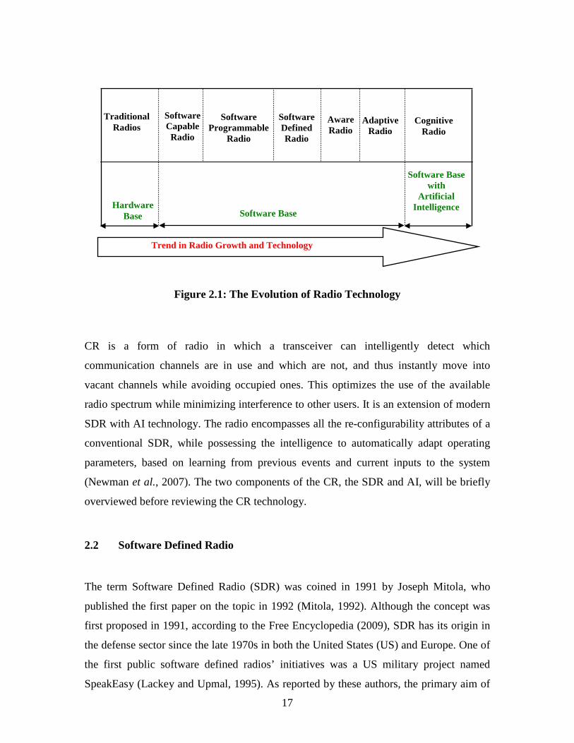
2.1 Radio Evolution Technology
Historically, radios have been fixed-point designs (Fette, 2006). However, over the last
decade, the design and implementation of wireless devices has undergone a substantial
transition from pure hardware-based radios to radios that involve a combination of
hardware and software. The functions that were formerly carried out by hardware can
now be performed by software, and the new functionality can easily be deployed on a
radio by simply updating the software running on it. Part of this change has ushered in
the advent of SDR, which is currently standard radio in the military arena and is gaining
favour in academic and commercial environments because of its ability to support
wireless communication research and implementation of real-world radio system.
Unlike the traditional radio devices that had fixed design and configuration, emerging
designs are allowing for much more flexibility in these areas. The culmination of this
additional flexibility produced the software capable radio, which later transitioned into
the software programmable radios that gave birth to SDR (Polson, 2004). The next step
along this path yielded the aware radio and the adaptive radio (Polson, 2004). In the
same vein, a more recent development has been the advent of CR. The transition in the
radio technology is illustrated in Figure 2.1.
17
Figure 2.1: The Evolution of Radio Technology
CR is a form of radio in which a transceiver can intelligently detect which
communication channels are in use and which are not, and thus instantly move into
vacant channels while avoiding occupied ones. This optimizes the use of the available
radio spectrum while minimizing interference to other users. It is an extension of modern
SDR with AI technology. The radio encompasses all the re-configurability attributes of a
conventional SDR, while possessing the intelligence to automatically adapt operating
parameters, based on learning from previous events and current inputs to the system
(Newman et al., 2007). The two components of the CR, the SDR and AI, will be briefly
overviewed before reviewing the CR technology.
2.2 Software Defined Radio
The term Software Defined Radio (SDR) was coined in 1991 by Joseph Mitola, who
published the first paper on the topic in 1992 (Mitola, 1992). Although the concept was
first proposed in 1991, according to the Free Encyclopedia (2009), SDR has its origin in
the defense sector since the late 1970s in both the United States (US) and Europe. One of
the first public software defined radios’ initiatives was a US military project named
SpeakEasy (Lackey and Upmal, 1995). As reported by these authors, the primary aim of
Software Capable Radio
Traditional Radios
Software Programmable
Radio
Software Defined Radio
Aware Radio
Cognitive Radio
Hardware Base Software Base
Software Base with
Artificial Intelligence
Trend in Radio Growth and Technology
Adaptive Radio
18
the SpeakEasy project was to use programmable processing to emulate more than ten
existing military radios, operating in frequency bands between 2 and 2000 MHz. Another
designed goal of the radio, as reported, was to easily be able to incorporate new coding
and modulation standards in the future, so that military communications can keep pace
with advances in coding and modulation techniques.
Conventionally, software defined radio is a radio communication system where
components that have typically been implemented in hardware, like mixers, filters,
amplifiers, modulators/demodulators, detectors and so forth, are instead implemented
using software on a personal computer (PC) or other embedded computing devices (Free
Encyclopedia, 2009).
According to Lackey and Upmal (1995), a SDR consists of the same basic functional
blocks as any digital communication systems. However, SDR lays new demands on many
of these blocks in order to provide multiple bands, multiple service operation and re-
configurability needed for supporting various air interface standards. In order to achieve
this flexibility, the boundary of digital processing should be moved as closely as possible
to antenna, while specific integrated circuits that are used for baseband signal processing,
need to be replaced with programmable implementations (Salcic and Mecklenbrauker,
2002). The idea behind SDR is to do all the modulation and demodulation with software,
instead of using dedicated circuitry.
In SDR, like the traditional radio, the signal is still being received by an antenna.
However, in SDR, the signal is digitally converted to a sequence of numbers representing
the value of the signal at regular time intervals (Katz and Flynn, 2009). These digital
values are then processed in software, while the resulting output can then be converted
back into audio, video or remaining data. The waveforms in SDR are therefore generated
as sampled digital signals, converted from digital to analog via a wideband Digital-to-
Analog Converter (DAC). The receiver similarly employs a wideband Analog-to-Digital
Converter (ADC) that extracts, down-converts, and demodulates the receive waveform or
signal using software built into a general-purpose processor or PC (Bedell, 2005). The
radio employs a combination of techniques that include multiband antennas and RF
conversion; wideband ADC and DAC conversion and the implementation of Intermediate
19
Frequency (IF), baseband and bit stream-processing functions in general-purpose
programmable processors, as shown in Figure 2.2.
Figure 2.2: Software Defined Radio Communication System
2.3 Implementation of Software Defined Radio
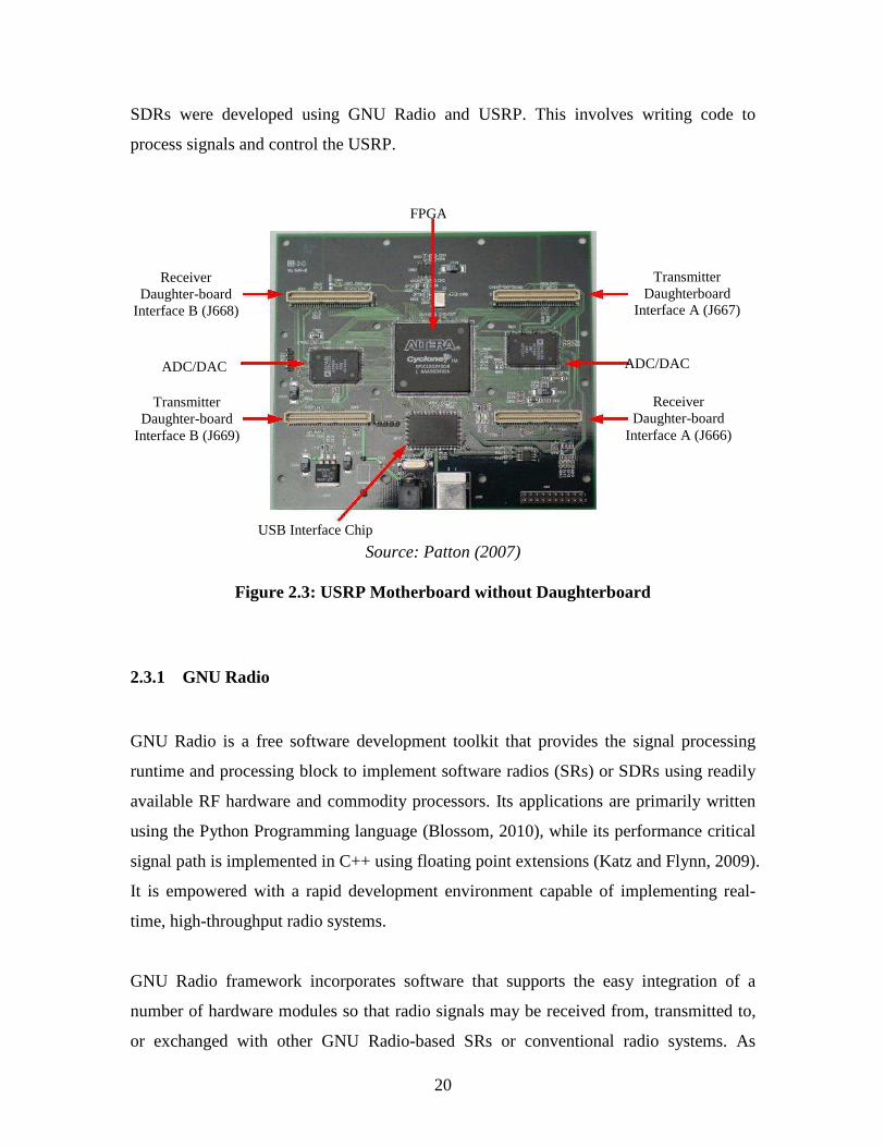
Figure 2.2 shows a typical block diagram for a software-defined radio. It implementation
involves using GNU Radio and the Universal Software Radio Peripheral’s (USRP)
motherboard and its associated daughterboard. The USRP motherboard provides the
ADC/DAC and Field Programmable Gate Array (FPGA) functionality, while
daughterboard attached to the USRP motherboard provides the frequency translation
functionality of the RF front-end (FE). The picture of a USRP motherboard with the
basic daughterboard’s slots is shown in Figure 2.3. The daughterboard’s slots are labeled
J66X (where X = 6, 7, 8 and 9).
There are number of experimental SDR platforms that have been developed to support
individual research projects. A selection of these platforms included (Minden et al., 2007;
Polydoros et al., 2003; Mishra et al., 2005; Adachi et al., 2007). These experimental
Receive RF Front-End
ADC Personal
Computer
Receive Signal Path
Transmit RF Front-End DAC
FPGA Personal
Computer
Transmit Signal Path
USRP (MOTHERBOARD) GNU RADIO DAUGHTERBOARD
Antenna
Antenna
FPGA Data out
Data in
20
SDRs were developed using GNU Radio and USRP. This involves writing code to
process signals and control the USRP.
Source: Patton (2007)
Figure 2.3: USRP Motherboard without Daughterboard
2.3.1 GNU Radio
GNU Radio is a free software development toolkit that provides the signal processing
runtime and processing block to implement software radios (SRs) or SDRs using readily
available RF hardware and commodity processors. Its applications are primarily written
using the Python Programming language (Blossom, 2010), while its performance critical
signal path is implemented in C++ using floating point extensions (Katz and Flynn, 2009).
It is empowered with a rapid development environment capable of implementing real-
time, high-throughput radio systems.
GNU Radio framework incorporates software that supports the easy integration of a
number of hardware modules so that radio signals may be received from, transmitted to,
or exchanged with other GNU Radio-based SRs or conventional radio systems. As
USB Interface Chip
Transmitter
Daughterboard Interface A (J667)
ADC/DAC
Receiver Daughter-board
Interface A (J666)
Receiver Daughter-board
Interface B (J668)
ADC/DAC
Transmitter Daughter-board
Interface B (J669)
FPGA
21
mentioned above, GNU Radio uses a modular block-based architecture with a hybrid
Python/C++ programming model. This combination of Python and C++ provides a
convenient and high performance platform for developers to use in the development of
SR systems (Troxel et al., 2008). According to these authors, one of the features of the
GNU Radio framework is an extensive library of pre-defined and tested functional blocks.
The essence of these blocks is to provide signal processing functionality, encapsulate
sources and sinks of data, as well as providing simple type conversions. According to
them, the blocks are written in C++ with an automatic generated Python wrapper or
interface that allows them to be manipulated, connected and utilized in Python.
GNU Radio software typically consists of four different elements: Sources, Sinks, Flow
graphs and Schedulers.
2.3.1.1 Gnu Radio Sources
Normally, typical GNU Radio sources usually have at least one source. Each source
forms the head of a processing chain or flow graph. A good example of a GNU Radio
source is USRP radio. The USRP radio is a radio FE that can be connected to a computer
via a USB 2.0 or Gigabit Ethernet. USB 2.0 is used for connecting USRP version 1 or
USRP1 to PC while Gigabit Ethernet is used for USRP version 2 or USRP2.
2.3.1.2 Gnu Radio Sinks
Like GNU Radio sources, typical GNU Radio will normally have a least one sink. Each
sink is the tail of a flow graph. An example of a sink is a sound card.
2.3.1.3 Gnu Radio Flow Graphs
A GNU Radio also has a flow graph. The flow graph links together each source and sink
pair as well as any intermediate blocks. The intermediate block(s) is or are required to
transform the data stream from a source into a format that is understandable by the sink.
A good example of such conversion is the conversion of an FM radio signal that is
received by a USRP into an audio signal that can be played through a sound card.
22
2.3.1.4 Gnu Radio Schedulers
A scheduler of a GNU Radio is associated with each active flow graph. The essence of
each scheduler is to move data through its flow graph. A scheduler iterates through the
blocks in the flow graph in order to identify blocks’ conditions per time. In its iteration
process, it will discover blocks that have sufficient data on their input(s) and sufficient
data on their output(s), it will then trigger the processing function for those blocks to
enable it to process data. Figure 5.4 shows a typical example of GNU Radio application
with these four components.
2.3.2 Universal Software Radio Peripheral
The common hardware platform to run GNU Radio on is the USRP. USRP is a device
that enables the creation of a SDR (Gahadza et al., 2009), using any computer with either
a USB 2.0 port or Gigabit Ethernet port depending on the version of USRP. With
different plug-on daughterboards nowadays, it is now possible to use USRP on different
radio frequency bands. A good example of USRP is Ettus’ USRP that allows general-
purpose computers to function as a high bandwidth SRs.
The USRP1 motherboard for instance, contains four 12-bits 64M samples/sec ADCs, four
14-bit 128M samples/sec DACs, an FPGA for IF up/down conversion, and a
programmable USB 2.0 controller to transfer control signals and baseband data sequences
between the host and the hardware. The motherboard can support up to two pairs of
transmitter/receiver (Tx/Rx) radio front ends in the form of daughterboards. Figure 2.4
shows a simple block diagram of USRP1.
There are multiple daughterboards options for different frequency bands. XCVR2450
transceiver daughterboards in junction with USRP2 are employed in this research work.
The USRP2 full description and mode of operation are presented in Appendix B of this
thesis.
23
Figure 2.4: USRP1 Block Diagram
2.4 Artificial Intelligence Techniques in Cognitive Radio
The heart of a CR’s application is in its ability to improve performance through learning.
This behavioral capability is achieved by the Artificial Intelligence Technique (AIT)
associated with CR. Artificial Intelligence is a field that is concerned with the design and
development of an algorithm that enables computer to learn. It is suitable for situations
based on experience, as they learn by example and act by analogy.
In CR, the integration of a learning engine has been established as very important
(Tsagkaris, et al., 2008; Katidiotis, et al., 2010). This has led to the proposal of different
intelligence algorithms for CR in literature. For instance, a cognitive engine developed at
Virginia Tech was developed using a Genetic Algorithm (GA). Their simulation results
validate that their GA implementation does change the transmission parameters to
ADC
ADC Receive
Daughterboard
FPGA
FX2 USB 2
Controller
ADC
ADC
Receive
Daughterboard
DAC
DAC Transmit
Daughterboard
DAC
DAC
Transmit
Daughterboard
24
different settings (Maldonado et al., 2005; Rondeau et al., 2004). In a similar research
conducted by Newman et al. (2007), GA was equally employed. Their work goes beyond
only demonstrating GA output selection, but also provides the numerical analysis of the
relationships between the environmental parameters and the transmission parameters.
Several other AI methods have been employed in the implementation of a cognitive radio
engine. A few of such methods are rule-based systems (Newman, 2008), case-based
reasoning (He et al., 2009), fuzzy logic (Shatila et al., 2009), and neural networks
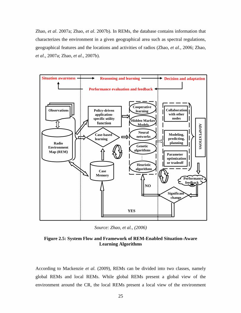
(Tsagkaris, et al., 2008). A schematic diagram of the AI cognitive radio-learning
algorithm employed by Zhao et al. (2006) is shown in Figure 2.5. The AI cognitive radio-
learning algorithm is referred to as a Radio Environment Map (REM) enabled situation-
aware learning algorithm. It comprises both a high-level and low-level learning loop. The
high-level loop is based on case-based learning/reasoning, which leverages various
learning algorithms to select the most appropriate learning method for the current radio
scenario. The low-level loop is responsible for optimizing the corresponding parameters
used in the specific learning algorithm.
2.5 Cognitive Engine
The Cognitive Engine (CE) is the intelligence system behind a CR or a node in a
Cognitive Network (CN). The CE combines sensing, learning and optimization to control
the CR or CN. A distinctive feature of CRs is their capability of making decisions and
adaptations based on past experience, on current operational conditions and possibly also
on future behaviour predictions (Mackenzie et al., 2009). According to these authors, an
underlying aspect of this concept is that CRs must efficiently represent and store
environmental and operational information in databases. These resulting databases, which
can be individual or shared, enable different functionalities of the CE. A possible
embodiment of such databases is discussed in form of REMs.
The application of REMs to CR systems was first proposed in the context of unlicensed
wireless wide area networks in Batra et al. (2004) and Krenik and Batra (2005). A
detailed study of the use of REMs by different CEs is discussed in (Zhao et al., 2006;
25
Zhao, et al. 2007a; Zhao, et al. 2007b). In REMs, the database contains information that
characterizes the environment in a given geographical area such as spectral regulations,
geographical features and the locations and activities of radios (Zhao, et al., 2006; Zhao,
et al., 2007a; Zhao, et al., 2007b).
Source: Zhao, et al., (2006)
Figure 2.5: System Flow and Framework of REM-Enabled Situation-Aware Learning Algorithms
According to Mackenzie et al. (2009), REMs can be divided into two classes, namely
global REMs and local REMs. While global REMs present a global view of the
environment around the CR, the local REMs present a local view of the environment
Collaboration with other
nodes
Parameter optimization or tradeoff
AD
AP
TA
TIO
NS
Significant change
YES
NO
Case-based learning
Case Memory
Policy-driven application-
specific utility function
Radio Environment Map (REM )
Observations
M
Performance feedback
Modeling, predicting, planning
Cooperative learning
Hidden Markov Models
Neural networks
Genetic algorithms
Heuristic algorithms
Situation awareness Reasoning and learning Decision and adaptation
Performance evaluation and feedback
26
around the CR. A source of global REM is usually the network infrastructure, while a
local REM is usually obtained, for example, by each radio from its own spectrum sensing
and by monitoring transmissions of nearby CRs and Primary Users (PUs). The
information in REMs is vital, as CRs uses it to optimize their transmit waveforms and
other parameters across the protocol stack.
2.6 Area of Application of Cognitive Radio
Technology is futile without its application. Out of many applications of CR, DSA has
been the most recognized application of CR. DSA is a decentralized approach to
spectrum allocation policy that allows a communication device to operate on any unused
spectrum. In this new paradigm, unlicensed or secondary users can opportunistically
operate in an unused licensed spectrum, as long it does not cause interference to the
licensed or primary users, thereby increasing the efficiency of spectrum utilization.
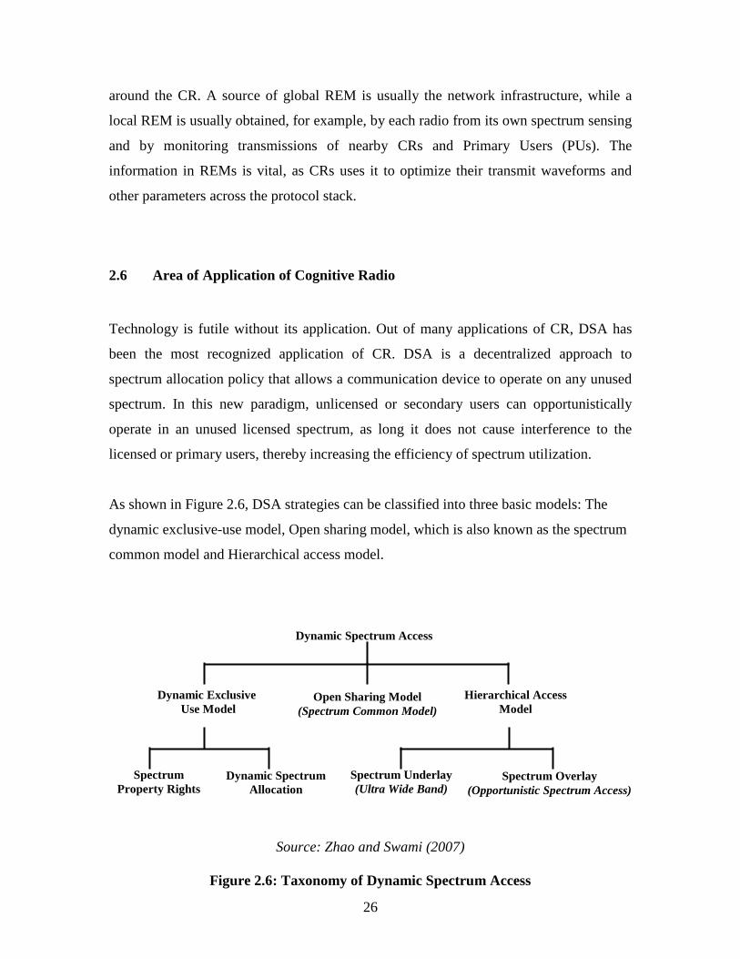
As shown in Figure 2.6, DSA strategies can be classified into three basic models: The
dynamic exclusive-use model, Open sharing model, which is also known as the spectrum
common model and Hierarchical access model.
Source: Zhao and Swami (2007)
Figure 2.6: Taxonomy of Dynamic Spectrum Access
Spectrum Overlay (Opportunistic Spectrum Access)
Dynamic Spectrum Access
Dynamic Exclusive Use Model
Open Sharing Model (Spectrum Common Model)
Hierarchical Access Model
Spectrum Property Rights
Dynamic Spectrum Allocation
Spectrum Underlay (Ultra Wide Band)
27
2.6.1 Dynamic Exclusive Use Model
This model maintains the basic structure of the current spectrum allocation policy,
whereby spectrum bands are licensed to users for exclusive use. This method of spectrum
allocation policy has led to many successful applications, like broadcasting and cellular,
which can be cited as evidence by the proponents of spectrum property rights (Ileri and
Mandayam, 2008). However, the method has also been criticized as inefficient in the
overall use of spectrum. For instance, a recent report presenting statistics regarding
spectrum utilization show that only about 13% of the allocated spectrums were utilized
(McHenry and McCloskey, 2004). In addition to the problem of underutilization
characterizing the current fixed spectrum allocation policy, the inherent political
inefficiency of government controllers also plays a role in the poor effectiveness of the
current allocation policy.
To correct this problem, the proposed idea is to introduce flexibility to spectrum access.
Two approaches have been proposed under this model. The first approach is spectrum
property rights (Coase, 1959; Hatfield and Wieser, 2005). As reported by Zhao and
Swami (2007), this approach allows licensees to sell and trade spectrum, and to freely
choose technology.
The second approach is dynamic spectrum allocation (Xu et al., 2000), which was
brought about by the European DRiVE project. Its aim, as reported by Zhao and Swami
(2007), was to improve spectrum efficiency through dynamic spectrum assignment by
exploiting the spatial and temporal traffic statistics of different services. Similar to the
current fixed spectrum allocation policy, this strategy allocates, at a given time and
region, a portion of the spectrum to a radio access network for its exclusive use. Based on
an exclusive-use model, it has been established that both spectrum property rights and
dynamic spectrum allocation cannot eliminate the current problem of spectrum
underutilization with increasing wireless traffic (Zhao and Swami, 2007).
28
2.6.2 Open Sharing Model
The open sharing model, which is also referred to as spectrum commons model (Lehr and
Crowcroft, 2005), puts all users on equal footing (Zhao and Swami, 2007), provided that
users obey specific rules similar to current unlicensed Industrial, Scientific and Medical
(ISM) radio bands. According to Zhao and Swami (2007), advocates of this model draw
support from the phenomenal success of wireless services operating in the current
unlicensed ISM radio band, like Wireless Fidelity (Wi-Fi).
2.6.3 Hierarchical Access Model
Under this radio spectrum access model, the radio spectrum is viewed as having a
primary or licensed user, as well as a secondary or unlicensed user. The model is
considered a hybrid of the other two models previously discussed. It is fundamentally
different from the other two models in both technical and regulatory aspects. The
fundamental idea of the model is to open licensed spectrum to unlicensed users, but with
Interference Avoidance (IA) to the licensed users. Based on this concept, two different
approaches to radio spectrum sharing between licensed and unlicensed users have been
considered, namely spectrum underlay and spectrum overlay, which are further discussed
below.
2.6.3.1 Spectrum Underlay
The spectrum underlay technique is a spectrum access system whereby signals with a
very low spectral power density can coexist as secondary users (SUs) with the PUs of the
frequency bands. The technique imposes severe restraints on the transmission power of
SUs so that they operate below the noise floor of PUs. An UWB transmitter that uses this
technology usually spreads its transmitted signal over a wide frequency band in order to
achieve short-range high data rate with extremely low transmission power. The detection
component for PUs is not required in spectrum underlay, since the energy of the
transmission signals by the SUs are spread over a very wide frequency range, thus only
negligibly increasing the interference temperature (Berthold et al., 2007).
29
However, according to Khoshkholgh et al., (2010), satisfying the interference constraint
is technically challenging, since the interference power constraints associated with
underlay access strategy only allows short-range communications (Srinivasa and Jafar,
2007). In addition, in underlay spectrum sharing, the secondary user must satisfy the
interference threshold condition even when the primary user is idle. During this idle
period, fulfilling the interference constraint limits the transmission power of the
secondary user, hence reducing its achievable transmission capability. More so, in
underlay access strategy, the achievable capability of the secondary user is further
reduced during the busy periods of the primary user because of the interference imposed
by the primary user’s activity at the secondary user’s receiver. In order to tackle these
aforementioned issues, overlay spectrum sharing was proposed.
2.6.3.2 Spectrum Overlay
The spectrum overlay technique is a spectrum access system whereby a SU uses a
spectrum band from a PU only when it is free. Unlike the underlay system, which hides
the transmission signal under the noise level of the PU, overlay system must have the
capability of dynamic spectrum access, as they must work dynamically around the
licensed system’s allocation. This technique is based on a detection and interference-
avoidance mechanism. This mechanism requires the SU to sense the frequency spectrum
and thus, if a PU is active, the channel will not be used.
The spectrum overlay access strategy was first envisioned by Mitola (1999) under the
term spectrum pooling. It was later investigated by the Defense Advance Research
Projects Agency neXt Generation (DARPA XG) program under the term OSA (Zhao and
Swami, 2007). Unlike the spectrum underlay, this radio spectrum access strategy does not
impose severe restrictions on the transmission power of SUs, but rather there are
restrictions on when and where SUs can transmit.
Spectrum overlay, according to Fujii and Suzuki (2005), can be applied in either temporal
or spatial domain. When using the radio spectrum in temporal domain, SUs aim to exploit
temporal spectrum opportunities resulting from the busy traffic of primary users. On the
other hand, when the radio spectrum is used in spatial domain, SUs aim to exploit
30
frequency bands that are not used by PUs in a particular geographic area. This unused
portion of the licensed spectrum is known as ‘white space’ or ‘spectrum hole’. Haykin
(2005) defines it as, “a band of frequencies assigned to a primary user but at a particular
time and specific geographic location the band is not being utilized by that user”. The
special radios that are enablers of OSA or DSA that can use spectrum holes in an
opportunistic fashion are known as cognitive radios.
2.7 Cognitive Radio
A cognitive radio is a new paradigm in radio communications that promises an enhanced
utilization of the limited radio spectral resource (Simeone et al., 2007). According to
these authors, the basic idea is to employ a hierarchical model, where both primary and
secondary users coexist in the same frequency spectrum. Unlike the conventional radio
that is only allowed to operate in a designated spectrum band due to regulatory
restrictions, CR has the capability to operate in different spectrum bands. It is a form of
wireless communication system in which a transceiver can intelligently detect which
communication channels are in use and which are not in use, and instantly move into
vacant channels while avoiding occupied ones.
The term ‘cognitive radio’ was first used in Mitola III and Maguire (1999). It is a term
that defines the wireless system that can sense, be aware of, learn from, and adapt to the
surrounding environment according to inner and outer stimuli. The radio provides a
tempting solution to the spectral crowding problem by introducing the opportunistic
usage of frequency bands that are not occupied by their licensed users. The radio concept
proposes to furnish the radio system with the abilities to measure and be aware of
parameters related to the radio channel characteristics, availability of spectrum and power,
interference and noise temperature, available networks, nodes, and infrastructures, as well
as local policies and other operating restrictions (Arslan and Şahin, 2007).
Recently, CR has emerged as a prime candidate for exploiting the increasing flexible
licensing of wireless spectrum. The flexible licensing of radio spectrum was suggested as
31
the spectrum resources are facing both huge usage and demands with the rapid growth of
wireless services and applications in recent decades. This increase in both spectrum
usage and demands has led to the belief that scarcity of radio spectrum is due to the
emergence of new wireless services and applications. However, this misconception about
spectrum scarcity is being tempered by a recent survey by a Spectrum Policy Task Force
(SPTF) within FCC. The result of their survey shows that the actual licensed spectrum
under the current fixed spectrum allocation policy is largely underutilized in vast
temporal and geographic dimensions (FCC, 2002).
As reported by Letaief and Zhang (2007), a field spectrum measurement taken in New
York City showed that the maximum total spectrum occupancy is only 13.1% from 30
MHz to 3 GHz. A similar measurement result undertaken in an urban setting, reported by
Čabrić and Brodersen (2005), revealed a typical utilization of 0.5% in the 3-4 GHz band.
The authors reported that the utilization drop amounted to 0.3% in the 4-5 GHz band.
Another related survey’s result reported by Song et al. (2007) also showed that, on
average, there is only about 5.2% of the allocated spectrum below 3 GHz actually in use.
These exciting findings shed light on the problem of spectrum scarcity and motive a new
direction to solve the paradox between spectrum scarcity and spectrum underutilization.
A remedy to spectrum scarcity as a result of spectrum underutilization is then to improve
spectrum utilization by allowing secondary users to access underutilized licensed
frequency bands dynamically when and where licensed users are absent. The main
enabler of this opportunistic spectrum access, as mentioned above, is cognitive radio.
Based on its abilities to sense and adapt to different radio environments, cognitive radio
has been defined in various ways (Haykin, 2005; Akyildiz et al., 2006; Ghozzi et al.,
2006; Hamdi et al., 2007). For instance, it was defined in Akyildiz et al. (2006) as, “a
radio that can change its transmitter parameters based on interaction with the
environment in which it operates.” Similarly, Haykin (2005) defines CR as “an intelligent
wireless communication system that is aware of its surrounding environment (i.e., outside
world), and uses the methodology of understanding-by-building to learn from the
environment and adapt its internal states to statistical variations in the incoming radio
32
frequency (RF) stimuli by making corresponding changes in certain operating
parameters (e.g., transmit-power, carrier-frequency, and modulation strategy) in real-
time, with two primary objectives in mind:
• highly reliable communications whenever and wherever needed; and
• efficient utilization of the radio spectrum.”
For CR to operate in an interference-avoidance way, one of most critical components of
CR is spectrum sensing. By sensing and adapting to the environment, a CR is able to
utilize spectrum holes and serves its users without causing interference to the licensed
user. To ensure interference-free communication, different sensing and detection methods
have been proposed for detecting the presence of primary or licensed radio signals. These
different sensing and detection methods are reviewed in section 2.8.
2.8 Spectrum Sensing Techniques
Spectrum sensing is a key element in CR communications, as it should be firstly
performed before allowing unlicensed users to access an unused licensed spectrum. The
essences of spectrum sensing are two-fold: one to ensure CR or secondary user does not
cause interference to a PU and two, to assist CR or secondary user to identify and exploit
the spectrum holes for the required quality of service (Popoola and van Olst 2011c). This
sensing operation is a binary hypothesis-testing problem. The goal of spectrum sensing is
to decide between the following two hypotheses:
( ) ( )( ) ( ) ( )tntstxH
tntxH
+==
:
:
1
0 (2.1)
where, 0H denotes the absence of the primary user, 1H denotes the presence of the
primary user, ( )tx is the received signal at the cognitive radio, ( )ts is the transmitted
signal from the primary transmitter and ( )tn is the Additive White Gaussian Noise
(AWGN). The determination of the two hypotheses is called the spectrum sensing.
33
Generally, spectrum sensing techniques are classified into either non-cooperative or
cooperative. However, from the perspective of signal detection, sensing techniques are
classified into four broad categories (Akyildz et al., 2011). The first two broad categories
are coherent and non-coherent detection techniques. In coherent detection, a priori
knowledge of the primary users’ signals is required, which will be compared with the
received signal to coherently detect the primary signal. In non-coherent detection, no a
priori knowledge of primary users’ signals is required for coherent detection. The last
two broad categories, which are based on the bandwidth of the spectrum of interest for
sensing, are narrowband and wideband detection techniques. The classification of sensing
techniques is shown in Figure 2.7.
Source: Akyildz et al., (2011)
Figure 2.7: Classification of Spectrum Sensing Techniques
2.8.1 Non-cooperative Spectrum Sensing Method
An individual CR device or secondary user does the non-cooperative spectrum sensing
method locally. Each secondary user will sense the spectrum channel to detect the
presence or absence of a primary user. Since the sensing method does not involve
spectrum sensing results’ sharing, as well as final decision making, energy consumption
is very low compare to cooperative spectrum sensing where users consume significant
energy because of heavy communication. However, the detection accuracy of the method
Spectrum Sensing Techniques: Cooperative or Non-cooperative
Narrowband Coherent Non-Coherent Wideband
Cyclostationary Detection
Matched Filter Detection
Wavelet Detection
Compressed Detection
Energy Detection
34
is very low compared to the cooperative method. This is because poor channel conditions
do affect single user spectrum sensing results (Lee and Wolf, 2008).
2.8.2 Cooperative Spectrum Sensing Method
Unlike non-cooperative spectrum sensing methods, where an individual cognitive radio
surveys the spectrum to gather information, the cooperative spectrum sensing method
usually involves two or more cognitive radios working together. In this spectrum sensing
method, an individual cognitive radio or secondary user will perform local spectrum
sensing independently and then makes a decision. Thereafter, all the cognitive users will
forward their decisions to a common receiver or Master Node (MN). The common
receiver will combine these decisions and makes a final decision to infer the presence or
absence of the primary user in the observed frequency band.
In general, activities in cooperative spectrum sensing can be summarized in three basic
steps as follows:
• Step I: Each cognitive radio performs its own local spectrum sensing
measurement independently and then makes a binary decision on whether the
primary user is present or not.
• Step II: All the cognitive radios forward their decisions to the MN or common
receiver.
• Step III: The MN aggregates the cognitive radios binary decisions received using
an “OR” logic and finally makes a decision to either infer the presence or absence
of the primary user.
The primary idea of cooperative spectrum sensing is to enhance the spectrum sensing
performance by exploiting the spatial diversity in the observations of spatially located
secondary users. Since it is unlikely that all spatially distributed secondary users in a
cognitive radio environment will concurrently experience the fading or receiver
uncertainty problem. Hence, when users collaborate and share the spectrum sensing
35
results among themselves, the combined cooperative decision derived from the spatially
collected observations can overcome the deficiency of individual observation of each
secondary user. This is why the cooperative spectrum sensing method has been observed
as an effective method to combat fading and shadowing, as well as mitigating the
receiver-uncertainty problem in a cognitive radio environment (Akyildz et al., 2011;
Mishra et al., 2006).
Architecturally, cooperative spectrum sensing is categorized into three classes based on
how cooperating cognitive radio users share the sensing information or data in the
network (Akyildz et al., 2011; Popoola and van Olst, 2011a). The classes are namely
centralized, distributed and relay-assisted. The three classes of cooperative spectrum
sensing illustrated in Figure 2.8 are briefly discussed in the following subsections.
Adapted from: Popoola and van Olst (2011a)
Figure 2.8: Classification of Cooperative Sensing: (a) Centralized, (b) Distributed, and (c) Relay-assisted
2.8.2.1 Centralized Cooperative Spectrum Sensing
In centralized cooperative spectrum sensing, a central identity called the master node or
fusion centre controls the three steps involved in cooperative sensing described above. In
Figure 2.8(a), CR1 is the master node and CR2-CR6 are the cooperative cognitive radio
(b)
CR1
CR2 CR3
CR4
PU
Reporting Channels
Sensing Channels
(a)
CR2
CR3
CR4
CR5
PU
(c)
Sensing Channels
Reporting Channels
CR1 (MN)
CR1 (MN) CR2
CR3
CR4
CR5
PU
Sensing Channels
Reporting Channels
CR6 CR6
36
users performing local sensing and reporting the results back to CR1. CR1 or MN collects
sensing information from CR2-CR6, identifies unused spectrum and broadcasts the
information to CR2-CR6.
2.8.2.2 Distributed Cooperative Spectrum Sensing
Unlike centralized cooperative sensing, distributed cooperative sensing, as shown in
Figure 2.8(b), does not rely on a MN for making the final cooperative decision. In this
cooperative sensing, after local sensing, the cognitive nodes CR1-CR4 share the local
sensing results amongst each other, but they make their own decisions as to which part of
the spectrum they can use. If there is no clear decision after this initial process, cognitive
radio users send their combined results to other users and repeat the sensing process until
the algorithm is converged and a decision is reached (Akyildz et al., 2011). The
disadvantage of distributed cooperative sensing is a decision delay possibility because
several iterations may be involved to reach a unanimous cooperative decision.
Maximum PSD of normalized centered amplitude, standard deviations of normalized centered amplitude, phase and frequency, standard deviations of direct value of instantaneous amplitude, standard deviations of the normalized instantaneous frequency, evaluated over the non-weak segment of the intercepted signal and maximum PSD of the normalized instantaneous frequency of the intercepted signal
2ASK, 4ASK, MSK, 2FSK, 4FSK, 2PSK, 4PSK
AWGN
Dobre et al., (2003)
Eighth-order cyclic cumulants of the received signal
BPSK, QPSK, 8PSK 4ASK, 8ASK, 16QAM, 64QAM, 256QAM
AWGN
Yu et al., (2003)
Discrete Fourier Transform (DFT) of the received signal
2FSK, 4FSK, 8FSK, 16FSK, 32FSK
AWGN
Dobre et al., (2004)
Eighth-, sixth-, and fourth-order cyclic cumulants of the received signal
4QAM,16QAM AWGN, impulsive noise
Zadeh et al., (2006)
Normalized eighth-order moments and cumulants of the received signal
Maximum PSD of normalized centered amplitude, standard deviations of normalized centered amplitude, phase and frequency
AM, FM, DSB, SSB (LSB, USB), CW4
AWGN
Wu et al., (2008)
Normalized fourth-order cumulants of the received signal
BPSK, QPSK AWGN and Multipath Fading
Source: Dobre et al.(2007)
1These are the modulation schemes used in the original papers. 3 Star-8QAM is a star shaped M-QAM modulation where M = 2n (M = 4, 8, 16, etc, n is the number of bits per one symbol). 4If the signal has no phase information and no amplitude information, it is called a CW signal. In this case, the instantaneous phase is a linear function of time and the instantaneous amplitude is constant, meaning that the CW signal has no useful information; no amplitude and no phase information.
66
In contrast to the DT approaches, the PR methods may be non-optimal, but simple to
implement and can often achieve the nearly optimal performance, if carefully designed.
Furthermore, the PR methods can be robust with respect to the aforementioned model
mismatches. In addition, observation from Table 2.4 and Table 2.5 revealed that
classifiers developed using feature based PR methods were capable of handling or
classifying more modulation schemes when compared with classifiers developed using
likelihood-based DT approaches. Also, the high computational complexity involved in
likelihood-based DT approaches compared to the feature based PR classifiers does hinder
these types of classifiers from handling more modulation schemes. These capabilities of
feature-based PR classifiers over the likelihood-based DT approach were considered in
this thesis. Thus, the PR approach was used in developing the automatic modulation
classifiers for this research work. In this study, the maximum PSD of normalized
centered amplitude, standard deviations of normalized centered amplitude, phase and
frequency are used as the primary feature extraction keys for the three classifiers
developed. In all the three classifiers, an artificial neural network was used for the
development of the AMC. Details on the development of the three classifiers for this
research work were presented in chapter 3.
2.12 Artificial Neural Networks
Artificial Neural Networks (ANNs) are information-processing systems that have certain
performance characteristics in common with biological neural networks. They are
computational modeling tools that have recently emerged and found extensive acceptance
in many disciplines for modeling complex real-world problems (Liao and Wen, 2007;
Basheer and Hajmeer, 2000). They are defined as structures consisting of densely
interconnected adaptive simple processing elements called artificial neurons or nodes that
are capable of performing massively parallel computations for data processing and
knowledge representation (Hecht-Nielsen, 1990; Schalkoff, 1997). The main objective of
developing ANN-based computing, like neurocomputing, is to develop mathematical
algorithms that will enable ANNs to learn by mimicking information processing and
knowledge acquisition in the human brain (Basheer and Hajmeer, 2000).
67
Though ANNs are drastic abstractions of biological neural network, the idea of ANNs is
not to replicate the operation of the biological systems, but simply to make use of what is
known about the functionality of the biological neural networks for solving complex
problems. According to Basheer and Hajmeer (2000), the attractiveness of ANNs comes
from the remarkable information processing characteristics of the biological neural
networks, namely non-linearity, high parallelism, robustness, fault and failure tolerance,
learning, ability to handle imprecise and fuzzy information and their capability to
generalize (Jain et al., 1996).
Artificial models possessing these processing characteristics of the biological neural
networks are desirable firstly because nonlinearity allows a better fit to the data; secondly
because high parallelism implies fast processing and hardware failure tolerance; thirdly
because learning and adaptivity allow the system to update or modify its internal
structure in response to the changing environment, and lastly because generalization
enables application of the model to unlearned data.
The main features of ANNs are that they have the ability to learn complex nonlinear
input-output relationships, use sequential training procedures, and adapt themselves to the
data. Based on these characteristics, an ANN has emerged as an important tool for
classification, which is one of the most frequently encountered decision-making tasks of
human activity. Usually, a classification problem occurs when an object needs to be
assigned into a predefined group or class based on a number of observed attributes related
to that object. Many problems in science, engineering, business and medicine can be
treated as classification problems. Common examples include character recognition,
speech recognition, quality control, modulation scheme recognition, medical diagnosis,
fraud and bankruptcy prediction to mention a few.
Recent research activities in neural classification have established that ANNs or simply
neural networks (NNs) are a promising alternative to various conventional classification
methods (Zhang, 2000). Its effectiveness as classifier has been empirically tested. Many
researchers (Packianather and Drake, 2005; Robert et al., 1997; Curram and Mingers,
1994; Huang and Lippmann, 1987) have carried out different performance comparisons
68
between NNs and conventional classifiers. Similarly, several computer experimental
evaluations of NNs for classification problems have been conducted under different
conditions (Patwo et al., 1993; Subramanian et al., 1993) confirming the superiority of
the NN classifier over other classifiers.
There are three main features that normally characterize an ANN:
(i) The pattern of connectivity among neurons, that is the ANN architecture
or structure;
(ii) The method of determining connection strengths i.e. ANN learning or
training algorithm; and
(iii) The activation functions of the network neurons.
2.12.1 Artificial Neural Network Architecture
ANNs contain a sequence of layers. Each layer consists of set of neurons, also called
Processing Elements (PEs). The arrangement of neurons or PEs into layers and the
connection patterns within and between layers give rise to the neural network architecture.
In neural network architecture, the first and the last layers are called input and output
layers (Suryanarayana et al., 2008).
To cope with nonlinearly separable problems, additional layer(s) of neurons are usually
placed in between the input layer and the output layer to form a Multi-Layer Perceptron
(MLP) architecture (Basheer and Hajmeer, 2000). This intermediate layer(s) of neurons,
are called hidden layer(s) and the nodes are called hidden nodes, because they do not
interact with the external environment. The inclusion of intermediate or hidden layer(s)
usually empowers the perceptron by extending its ability to solve nonlinear classification
problems. The number of hidden layers is usually not known; hence its number of
neurons only depends on the problem considered. Except for purely linear networks, the
more neurons used in the hidden layer, the more powerful the network (Demuth and
Beale, 2000). The number of both input and output neurons, on the other hand, are
usually problem dependent (Aggarwal et al., 2005).
69
In terms of architectural structure, neural networks are classified into two major
categories, namely Feed-Forward Neural Networks (FFNNs) and Recurrent Neural
Networks (RNNs). In a FFNN, the connections between neurons are in a feed-forward
manner. Similarly, the signal’s flow is usually from the input layer to the output layer in a
forward direction without feedback. The network is usually arranged in the form of layers.
The arrangement is such that there is no connection between the neurons within the same
layer and no feedback between layers.
A fully connected single layer and multilayer neural network, as shown in Figure 2.12 (a)
and (b) respectively are examples of FFNNs. On the other hand, the fully interconnected
multilayer neural network shown in Figure 2.13 is an example of RNN. The fundamental
feature of RNN is that the network usually contains at least one feedback connection.
In NNs, learning or training corresponds to the process by which the network’s
parameters, or weights, are adapted or adjusted through a mechanism of the presentation
of an input stimulus. It is an algorithm for finding suitable weights, W , and/or other
network parameters. NNs are usually trained by epoch. An epoch is a complete run when
all training examples are presented to the network and processed using the learning
algorithm only once.
Generally, when NNs are to be used, it is believed that the exact nature of the relationship
between inputs and outputs are not known, otherwise the user would have modeled the
system directly. Hence for NNs to model the relationship between the inputs and outputs,
they need to learn the inputs and outputs relationship through training. There are three
types of training used in NNs, with different types of networks using different types of
training. These training types are supervised learning, unsupervised learning and
reinforcement learning. Supervised learning is the most common and is the training
method applied in this research work.
Hidden Layer Input Layer Output Layer
Propagating neuron Processing neuron
Inpu
t
Output
71
Supervised learning is widely used in problems which involve pattern recognition or
classification, approximation, control modeling and identification, signal processing and
optimization. Unsupervised learning schemes, on the other hand are mainly used for
pattern recognition, clustering, vector quantization, signal coding and data analysis while
reinforcement learning is usually used in control. More details about the three types of
learning methods in a neural network are presented in following subsections.
2.12.2.1 Supervised Learning
This learning method embeds the concept of a supervisor or teacher, who has the prior-
knowledge about the environment in which the network is operating. This prior-
knowledge is represented in form of a set of input-output samples or patterns. These
input-output samples or patterns are provided in form of input data and desired output or
target (Torrecilla et al., 2007). In order words, the desired output or target is the output
expected to be received from the given input data.
The input data is propagated forward through the network until activation reaches the
output neurons. The output from the network will be compared with the desired output. If
the output from the network agrees with the desired output, there will be no need to
change the network parameters. However, if the output from the network differs from the
desired output then there will be a need to adjust the network parameters to ensure that
the network gives the correct answer in the future when it is presented with the same or
similar input data. This adjustment of the network parameters is carried out by adjusting a
combination of the training pattern set and the corresponding errors between the desired
output and the actual network response.
This network parameters adjustment scheme is what is known as supervised learning or
learning with a teacher. It is being regarded as a closed-loop feedback system where the
error is the feedback signal. It is being done so that the network can emulate the system.
A diagrammatic representation of a supervised learning algorithm is shown in Figure
2.14. The environment in Figure 2.14 provides the input patterns to train the network.
72
Figure 2.14: Diagrammatic Representation of Supervised Learning Algorithm
In order to control the learning process, a criterion is needed to decide the time for
terminating the learning process. In supervised learning, an error measure, which
indicates the difference between the network output and the output from the training
sample, is normally used to control the learning process. This error measure is obtained
by the Mean Squared Error (MSE), which is mathematically expressed as:
2
1
||1∑
=
∧−=
N
xxxR yy
NE (2.24)
where N is the number of the pattern pairs in the sample, xy is the output part of the xth
pattern pair and xy∧
is the network output corresponding to the pattern pair x . The
error,E , is calculated afresh after each epoch, while the learning process terminates when
E is sufficiently small (Du and Swamy, 2006).
According to Du and Swamy (2006), error E can be made to decrease toward zero by
applying a gradient-descent procedure. The gradient-descent method converges to a local
minimum in a neighborhood of the initial solution of the network parameters. The least
mean square and back-propagation (BP), as reported by the authors, are the two early and
most popular supervised learning algorithms. The two of them are derived using the
Environment Neural
Network ∑
Supervisor
Error signal
Network output
Desired output
Input patterns
+
_
73
gradient-descent procedure. In this research work, the BP learning algorithm was used in
reducing the error.
2.12.2.2 Unsupervised Learning
Unlike supervised learning, the unsupervised or self-organized learning method does not
involve a supervisor or target values to evaluate the network performance in relation to
the input data set, as shown in Figure 2.15. The network is only provided with the input
data to teach itself depending on some structures in the input data. These structures may
be some form of redundancy in the input data or clusters in the input data. The learning
method is particularly suitable for biological learning, in that it does not rely on a teacher.
Figure 2.15: Diagrammatic Representation of an Unsupervised Learning Algorithm Like the supervised learning, an unsupervised learning method needs a criterion to
terminate the learning process. This is to prevent the learning process from continuing
indefinitely. In this regard, Du and Swamy (2006) reported that, Hebbian learning,
competitive learning and Kohonen’s self-organization maps are the three mostly used
unsupervised learning criteria. Generally unsupervised learning has been observed to be
slow to settle into stable conditions.
2.12.2.3 Reinforcement Learning
This learning method is half-way between the supervised and unsupervised learning
methods. It is distinguished from the other learning methods as it only relies on learning
from direct interaction with the environment, but does not rely on explicit supervision or
complete models of the environment as shown in Figure 2.16. In this learning method,
the network is provided with the input data. The activation will then be propagated
forward with additional information, such as a reinforcement signal, telling the network
Environment Neural Network
Input patterns
Network output
74
whether it has produced the desired output or not. If the network produces an output
different from the desired output, some adjustment of the network weights will be done
so that a desired output is obtained in the future presentation of that particular input. In
this learning method, the network’s output provides the environment with information
about how the neural network is performing.
Figure 2. 16: Diagrammatic Representation of Reinforcement Algorithm In the real sense, reinforcement learning is a special case of supervised learning (Barto et
al., 1983). It is useful for learning control strategies only from a performance index
without any teacher who instructs how to control a system at each moment. It is a
learning procedure that rewards the NN for its good output result and punishes it for a
bad output result. It is normally used in a situation where the correct output for an input
pattern is not available and there is need for developing a certain output. It is a less
powerful method when compare with supervised learning and sometimes requires a large
amount of time. Reinforcement learning teaches the network structure by trial-and-error
and is suitable for online learning (Barto et al., 1983; Kaelbling et al., 1996).
2.12.3 Transfer Function
An activation or transfer function is a function used to transform the activation level of a
neuron into an output signal. It determines how the state of a neuron and its internal
activation is going to be modified in order to produce the neuron output. They are
monotonically non-decreasing and present non-linearity associated with saturation (De
Castro and Timmis, 2002). The most common activation functions employed in artificial
neural networks are hard limit, linear, logistic, and log-sigmoid transfer functions.
Environment Neural
Network
Input patterns
Reinforcement signal
Network output
75
• The hard limit transfer function usually sets the output of the neuron to zero if the
function argument is less than zero, or one if its argument is greater than or equal
to zero.
• The linear transfer function usually set its output to its input.
• The log-sigmoid transfer function takes an input that has any value between plus
and minus infinity and squashes the output into the range 0 to 1, according to the
expression:
111
−+=
eu (2.25)
• The log-sigmoid (logsig), tan-sigmoid (tansig) and linear (purelin) transfer
functions are commonly used in multilayer networks that are trained using a BP
algorithm because these transfer functions are differentiable and also monotonic
increasing functions. Meaning that, the output of each function increases with
increase in its input value (Demuth and Beale, 2000).
In BP networks, one or more layers of sigmoid neurons are usually used as the hidden
layer, followed by an output layer of linear neurons. The multiple layers of sigmoid or
non-linear transfer functions allow the network to learn non-linear and linear
relationships between input and output vectors. On the other hand, the linear transfer
function at the output layer allows the network to produce values outside the range -1 and
+1. However, when it is desirable to constrain the outputs of a network to have values
between 0 and +1, then a sigmoid or non-linear transfer function, such as logsig, can be
used at the output layer. The mathematical definitions of commonly used activation
functions are presented in Table 2.6.
76
Table 2.6: Activation Functions
Function Definition Range Identity x ( )infinf, +−
Logistic 11
1−− e
( )1,0 +
Hyperbolic
xx
xx
ee
ee−
−
+−
( )1,1 +−
Exponential xe− ( )inf,0 +
Softmax
∑i
x
x
ie
e
( )1,0 +
Unit sum ∑
iix
x
( )1,0 +
Square root x ( )inf,0 + Sine ( )xsin ( )1,0 +
Ramp
+≥++<<−
−≤−
1:1
11:
1:1
x
xx
x
( )1,1 +−
Step
≥+<
0:1
0:0
x
x
( )1,0 +
2.13 Summary
The focus of this chapter was to present basic background to this thesis, as well as to
enlighten all classes of readers on some of the developmental history in radio technology
and terms that will be later employed in this thesis. To fulfill these objectives, the chapter
has provided an overview of radio evolution, which led to both digital radio realizations
and software radio capabilities. The inclusion of software in radio systems has made
possible software capable radio that processes radio signals digitally. In the pursuit of
flexibility, software programmable radio, which eventually gave birth to the SDR, is
currently a standard in the military domain and gradually gaining recognition in the
commercial world especially in an academic environment, as reviewed in Section 2.1.
77
In Sections 2.2 and 2.3, a detailed background on SDR and GNU Radio in the
development of CR was reviewed. Section 2.4 presented various AIT associated with CR,
while the intelligence systems behind CR or CN are reviewed in section 2.5. Sections 2.6
and 2.7 presented full reviews of CR applications. The sections also provided reviews on
the demerits of the current radio spectrum management policy and the suitability of
cognitive radio technology as a novel technology in solving spectrum management
problems. The DSA application, based on cognitive radio technology to enhance radio
spectrum efficiency, was fully reviewed.
Section 2.8 and Section 2.9 of this chapter focused on the analyses of various sensing and
detection techniques in the surveyed literature respectively. The review shows that none
of the available sensing and detection methods is capable of sensing and detecting all
forms of radio signals in the cognitive radio environment. An attempt to address this
challenge motivated this research work, which proposes an alternative sensing and
detection technique using AMC. The proposed sensing and detection method using AMC
was envisioned because all users of the radio spectrum make use of one form of
modulation scheme or another. Hence, the ability to accurately detect the modulation
schemes of radio signals is sufficient to confirm the presence of radio signal in a
cognitive radio environment.
Section 2.10 is therefore devoted to the in-depth reviews of both fundamental analog and
digital modulation schemes. In Section 2.11, a comprehensive review of AMC for
various fundamental analog and digital modulation schemes used in wireless
communications systems and applications was carried out. Section 2.12, concludes the
study literature review work with a comprehensive review on ANNs.
Finally, having observed the demerits of the various available spectrum sensing detection
methods in the surveyed literature, this research work is embarked upon finding a novel
technique for sensing and detecting all forms of radio signals in a cognitive radio
environment. The execution of the research work is presented in two phases. The first
phase involves the development of the AMR used using MATLAB ®. The second phase
involves the experimental development of the CRE using an USRP2 coupled with a
78
combined analog and digital AMR classifier developed in the first stage of the study. The
diagrammatic representation of the radio environment model for the study is shown in
Figure 2.17.
Figure 2.17: Cognitive Radio Environment Model
In order to ensure reliable and effective spectrum sensing, each SUS (secondary user
sensor), in Figure 2.17 will individually perform spectrum sensing and relay its decision
to the master node secondary user sensor (SUSMN). The SUSMN will finally broadcast the
condition of the spectrum to all the SUs connected to it for dynamic spectrum access. The
other function of the SUSMN is to determine the SU terminal or node to access the free
spectrum per time, while the SUS are continuing spectrum sensing. The SUSMN also
ensures even distribution of the spectral resources amongst the SUs.
The condition for DSA of licensed spectrum in this research work is based on non-
detection of any form of modulation scheme on any channel considered. This condition is
fulfilled by the in-built capability of the AMR incorporated into the developed CRE.
Therefore, the focus of the next chapter will be on development of automatic modulation
classifiers for the research work. The next chapter discusses details on how the feature
extraction keys used in developing the AMR classifiers for the research are obtained
using simulation. The chapter also provides in-depth information on how the three AMR
classifiers were developed using ANNs, as well as their individual performance.
Licensed Network
SUS
SUS
SUSMN
PU
PU
PU
PU
SU
SU
SU
79
CHAPTER 3
3.0 DEVELOPMENT OF AUTOMATIC MODULATION CLASSIFIERS
This chapter presents details on the development of the three automatic modulation
classifiers developed in this study. The developed classifiers are: analog automatic
modulation recognition (AAMR), digital automatic modulation recognition (DAMR) and
combined analog and digital automatic modulation recognition (ADAMR). The AAMR
was developed to discriminate between four of the best-known analog modulation
schemes, namely AM, DSB modulation, SSB modulation FM. The developed DAMR
was developed to discriminate between eight of the best-known digital modulation
schemes, which are:
- two symbol amplitude shift keying (2ASK);
- four symbol amplitude shift keying (4ASK);
- two symbol frequency shift keying (2FSK);
- two symbol phase shift keying (BPSK);
- four symbol phase shift keying (QPSK);
- orthogonal frequency division multiplexing (OFDM);
- sixteen symbol quadrature amplitude modulation (16-QAM); and
- sixty-four symbol quadrature amplitude modulation (64-QAM).
The combined ADAMR was developed to discriminate between twelve, four analog and
eight digital modulation schemes considered, as well as un-modulated noise. The
classifiers are feature based modulation recognition algorithms using statistical features.
The classifiers are developed using MATLAB. They are implemented in a hierarchical
approach to classify radio signals using the smallest amount of required data, while
simultaneously maximizing the reliability of the classifiers. The twelve simulated
modulation schemes were realized using MATLAB codes. In addition to the basic
MATLAB ® software, the Netlab Algorithm for pattern recognition was used in
developing the three classifiers.
80
This chapter’s focus, however, is not to develop a new feature extraction key algorithm
but simply to develop AMC classifiers that would be employed in developing the
spectrum sensing engine for the thesis. Hence, in developing the three developed
classifiers for the thesis, earlier existing feature extraction keys algorithms were
employed. However, the employed feature extraction keys algorithms were not from a
single study but from various studies based on the effectiveness of those feature
extraction keys.
3.1 Analog Classifier Development
The development of the three AMR classifiers for this research work involved three
different stages as shown in Figure 3.1. For the AAMR classifier, the four analog
modulation schemes employed were first simulated using MATLAB codes in the first
stage. In addition, in this first stage, the three feature keys that were used as input data
sets to the classifier to discriminate between the four analog modulation schemes were
extracted using MATLAB codes. The second step involved the development of the
classifier, while the third step was on the performance evaluation of the developed
classifier. Details on each of the three stages are presented in the following subsections.
Source: Azzouz and Nandi (1996a)
Figure 3.1: Functional Blocks for AMR Development
3.1.1 Pre-Processing Stage
This stage deals with the extraction of the feature keys used in discriminating between the
four analog modulation schemes considered. In an automatic modulation identification
study, finding the proper feature extraction keys is very important (Zadeh et al., 2006). In
the development of the AAMR for this research work, three feature keys were used to
*: Data’s second decimal points are approximate values extracted from graphs.
150
6.3 SSADA Proof of Concept Evaluation
Due to limitations of the USRP2 daughterboards availability, the tests results presented
above were carried out using an XCVR2450 daughterboard operating in an ISM
frequency band. Therefore, in order to extend the testing, as well as showcase the
practicability of the proposed spectrum sensing and detection method in other usable
frequency bands, the CE, which is the brain of the developed CRE, was further developed
in a graphical user interface called SSADA. The SSADA’s development was fully
described in chapter 5, while its performance is briefly examined in this chapter.
Additional information on the performance evaluation of SSADA is presented in
Appendix C. Meanwhile, its performance evaluation in a hypothetical television
frequency allocation table is presented below using two of its features. The two features
demonstrated are its spectrum scanning and cooperative gain optimization prediction’s
capabilities presented in section 6.3.1 and 6.3.2 respectively.
6.3.1 SSADA Spectrum Scanning Capability Test
A typical spectrum scanning result by the developed SSADA is presented here. Based on
the current radio spectrum allocation policy, the Television (TV) frequency bands shown
in Table 5.4 are randomly allocated among the six cities used. The frequency bands’
random allocation was carried out to conform to the current frequency allocation policy.
Figure 6.4 shows typical cooperative spectrum sensing for the hypothetical TV frequency
band. The algorithm scans each frequency band to detect spectrum holes in each band
before proceeding to the next band. The result shows that the developed SSADA
functions well, with a high capability of detecting occupied bands and spectrum holes
respectively in the TV frequency bands used to illustrate it capability.
151
Figure 6.4: A Section of Typical TV Frequency Bands Scanning Result
: Represent some cut off parts of the scanning result’s screen
152
Careful observation of the developed SSADA shows that, irrespective of the allocated
frequency bands for each of the locations, the developed SSADA is designed to scan the
overall frequency bands for each wireless service. This approach enables OSA or DSA
deployment in all the locations as the overall scanning of the spectrum provides
information on primary user activity on each channel per time period, and therefore
enhances overall optimal spectrum utilization. Further evaluations of the SSADA are
presented in Appendix C.
6.3.2 Sensing Time versus FFT size
The second evaluation test carried out on the developed SSADA is its capability of
predicting the appropriate setting of the FFT size (N), so as not to incur a cooperative
overhead. The parameter, N, was not considered in chapter 4, however, observation
shows that its indiscriminate selection can affect the sensing time and increase the
cooperative overhead. Considering Figure 6.5, which shows the plot of the sensing time
against N obtained from the developed SSADA, with value of N varying from 16 to
1024; the figure shows that the sensing time increases with increase in N. This is
expected since processing gain is proportional to FFT size N and observation or sensing
time (Čabrić et al., 2004). However, Figure 6.5 shows that indiscriminate choice of N
will increase the sensing time and cooperative overhead rather than increasing the sensing
accuracy. Thus, in this research work, FFT size of 32 was employed. The FFT size of 32
was chosen because values of FFT sizes above 32 only cause a sporadic increase in Ts.
This shows that the increase in N’s value above 32 only increases the sensing or
observation time, Ts, without enhancing the detection probability.
153
Figure 6.5: SSADA Sensing Time against FFT size N
6.4 Summary
In this chapter, the focus is on performance evaluation of the developed CRE for this
research work. The laboratory setup to evaluate the performance of the developed CRE
by determining its detection states and detection probabilities using various modulation
schemes at different SNR shows that primary aim and objectives of the research had been
achieved. Though the sensing time required for this sensing and detection method
varies from one modulation type to another, its high correct detection state with
negligible false and miss detection states is one of the significant advantages of the
proposed method. Its other advantage is its high average PD values that cut across all the
SNR values for all the modulation schemes considered.
In addition, the capability of the developed SSADA that could scan all the hypothetical
allocated frequency bands for the four wireless services within the country is an
indication that the CRE as developed, which incorporates implemented CE as its core,
can enhance OSA or DSA deployment in any part of the country. Similarly, since the
hypothetical allocated frequency bands can be replaced by any frequency bands of any
country, makes the developed CRE’s deployment applicable to any part of the world.
154
CHAPTER 7
7.0 RESEARCH SUMMARY AND CONCLUSION
This chapter concludes this thesis with a brief summary of the thesis and the
contributions of the work to the field of primary radios’ signals sensing and detection in a
cognitive radio environment. The chapter ends with recommendations on the adoption of
DSA as an alternative spectrum access strategy in mitigating the current challenge of
spectrum underutilization and enhancing the continued availability of radio spectrum for
future wireless devices.
7.1 Thesis Summary
The world as a whole is approaching the limits of the availability of useable radio
frequency for wireless communication, while at the same time the demand for and use of
radio spectrum for wireless services and applications are greatly increasing. Observations
have also shown that, as the demand for and use of the radio spectrum is increasing, so do
the challenges to the successful management of the radio spectrum using the current fixed
allocation policy. In light of this, there is a need to adopt an alternative radio spectrum
access strategy and management policy that would enhance both the management and
usage of radio spectrum in order to enhance radio spectrum availability for future
wireless devices. The aim of this research work, as stated in chapter 1, is to develop a
CRE that can sense and detect all forms of primary radio signals in a cognitive radio
environment. This is because the development of this type of radio engine that generates
little or no interference to primary users in a cognitive radio environment, such a radio
engine is one solution that can guarantee the general acceptance of cognitive radio
technology, which is a promising solution for overcoming radio spectrum scarcity and
underutilization currently experiencing worldwide.
In achieving this aim, a comprehensive literature review on conventional primary radio
detection methods in a cognitive radio environment was carried out in chapter 2. It was
155
during the literature survey that factors responsible for failure of most of these
conventional spectrum sensing and detection methods was discovered, as most of these
methods were developed based on features that are limited to certain types of radio
signals, instead of employing a feature that is common to all primary radio signals. This
shortfall was accounted for in this research work, by using an automatic modulation
identification methodology to develop this research work’s spectrum sensing and
detection method. The methodology was used because all radios using the radio spectrum
make use of one modulation or another.
Chapter 3 discussed in full the procedures involved in developing the Automatic
Modulation Recognition (AMR) classifier used for the research. The starting point for the
AMR classifiers’ development, which is the feature keys extraction process, was
presented in chapter 3. The chapter also contains detailed information on the development
and evaluation of the three AMR classifiers developed. In chapter 4, the sensing time
algorithm for enhancing cooperative spectrum sensing performance was developed.
Chapter 5 of this thesis was devoted to one of the major components of this research
work, which is on the development of a CRE to sense and detect a primary radio signal in
a cognitive radio environment. The importance of CRE in cognitive radio technology was
reviewed in section 2.5. Different AI schemes employed in developing previous CREs
were also reviewed in that section. The review of these schemes revealed their limitations,
such as non-resistance to noise, which was adequately taken care of in the ANN
employed for the development of the CRE in this research work.
The other major component of this research is the development of an SSADA or CE
using the JAVA programming language. The user-friendly interface program was
developed to provide a proof of concept evaluation of the developed CRE, where the
developed SSADA is its core brain. The SSADA incorporates the following three
modules:
- Preferred service and location for radio spectrum scanning and random
table of frequency allocation per geographical location;
156
- The plotting section, where the sensing time parameters selection for
optimizing cooperative spectrum sensing gain can be done; and
- The manual calculations section for calculating the spectrum sensing
time (Ts).
The three modules incorporated in the developed SSADA are shown in Figure C.1 in
Appendix C.
Testing of the developed CRE and SSADA using different performance criteria and
metrics was undertaken. Although the proposed sensing and detection method’s response
time varies with the modulation schemes, the overall results revealed that the developed
CRE and SSADA were versatile. In addition, the favouarble comparative analysis result
obtained when the results of the proposed sensing and detection method in this research
work was compared with the generally acclaimed best detection method in the literature
provides a good assessment of the proposed sensing and detection method in this research.
7.2 Conclusion and Recommendation
The dynamic spectrum access, which is one of the applications of cognitive radio
technology, has been observed as a promising solution to the problem of radio spectrum
scarcity and underutilization by introducing the opportunistic usage of licensed frequency
bands that are not efficiently utilized by licensed owners. Following the general belief
that spectrum sensing is the key functionality to enable DSA, this research work focused
on issues of spectrum sensing. The thesis discussed merits and demerits of most of the
current detection methods or algorithms presented in literature. After a careful, neutral
and constructive analysis of most of the current detection methods in literature, it showed
that none of the methods can adequately and reliably detect all forms of primary radio
signals in a cognitive radio environment. This leads to the novel detection method
proposed in this research work using an automatic modulation recognition method.
157
The implementation of this study’s detection method using both hardware and software
components has been fully discussed. Also the results obtained in this study, when
compared with other conventional detection methods, showed high reliability of the
proposed detection method in detecting all forms of primary radio signals in a cognitive
radio environment. Although the proposed sensing and detection method’s observation
time or sensing time varies with modulation schemes, the numerical result from the study
shows the significant performance of the proposed detection method, even at a low SNR
values, where the conventional detection methods usually perform poorly.
In addition to these, another significant contribution of this research work is the practical
implementation of the proposed detection method using practical and available
components. This study has shown that the practical development of a reliable detection
method is possible and attainable using AMR. The AMR, which is the core identification
feature employed in this detection method, has confirmed the preliminary investigated
discovery during the literature survey that most conventional detection methods in
literature perform poorly because the features used were not features common to all radio
signals like the modulation identification scheme employed in this study. The proposed
detection method in this research shows a favourable comparison with the energy
detection method, whereby signal energy content, which is also a feature common to all
radio signals, shows that a single spectrum sensing and detection method can only be
achieved when a feature common to all radio signals is employed in its development
rather than using features that are limited to certain signal types.
Another significant factor or contribution of this research work is the bedrock
information it has provided on how to improve cooperative spectrum sensing gain
without incurring a cooperative overhead. Numerical results from the study have shown
that not only does the detection method perform well, but that the overall objectives of
the research work have been achieved.
Based on the results obtained from this research work and the performance of the novel
spectrum sensing detection method proposed in this study, it is hereby recommended that
the adoption of an opportunistic spectrum access, also known as DSA, as an alternative
158
spectrum access strategy be adopted. The access strategy is proposed because it will not
only solve the current problem of radio spectrum underutilization, but will equally reduce
the current problem of radio spectrum scarcity. Furthermore, because the proposed
detection method in this thesis guarantees no interference amongst users of the spectrum,
which is the primary objective of the traditional fixed spectrum allocation policy, thus the
adoption of DSA will not compromise the performance of existing radio systems that will
continue to adopt the traditional radio spectrum regulation system with the
implementation of the novel detection method devised in this research work.
7.3 Future Work Recommendations
With the success recorded in this research work, there is guarantee now that the perceived
danger of interference due to DSA radio operation has been solved and the adoption of
DSA using CR technology for radio spectrum management and access is gradually
becoming a reality. However, some research work still needs to be done. The
recommended work is actually outside the scope of this research project but it is
recommended for future work so as to enhance the CRE developed in this research as
well as accelerating the immediate adoption of DSA. The future work recommended is as
follows:
• Firstly, future work needs to be carried out on how to incorporate an efficient and
adaptive channel access scheme that can support both dynamic channel selection
and power allocation in a cognitive radio environment to the CRE developed. To
achieve this, instead of the random allocation of the radio spectrum band by MN
in this study, game theory for spectral resources, such as power and spectrum
bands, allocation can be incorporated into the CRE developed. The use of game
theory was specified because of its inherent capability to check users that behave
in a selfish manner by seeking a performance advantage over other users at the
cost of overall network performance.
159
• Secondly, future work needs to be carried out on the developed ADAMR
classifier incorporated in the developed CRE in this thesis. This is to improve the
classifier operational time and the developed CRE detection time. Another
alternative work to this is to replace the ADAMR classifier employed in the
development of the CRE for this thesis with DAMR with better operational time
performance especially now that most systems and nations are shifting from
analog communication system to digital communication system. Furthermore, the
number of the modulation schemes can be increased to accommodate more
modulation schemes.
• Thirdly, comparative future work analysis on this thesis algorithm complexity and
that of energy method needs to be carried. This future work is essential as it will
provide basis for comparing the two spectrum sensing and detection methods on
their respective complexity, which is different from the comparative PD
performance analysis carried out in this thesis.
160
References
Abdi, A., Dobre, O.A., Choudhry, R., Bar-Ness, Y., and Su, W. (2004). Modulation classification in fading channels using antenna arrays. In Proceedings of IEEE Military Communications Conference 2004 (MILCOM 2004), vol. 1, pp. 211-217. Abdullah, K., Hinai, N.A., Sadik, A.Z., and Hussain, Z.M. (2009). Circular 16-QAM modulation scheme for wavelet and Fourier based OFDM systems. In Proceedings of the 5th IEEE Gulf Cooperation Council (GCC) Conference, Kuwait City, pp. 1-6. Adachi, F., Wakana, H., Morikawa, H., Kuroda, M., Harada, H., Isobe, S., Miura, R. and Ogawa, H. (2007). Network and access technologies for new generation mobile communications - overview of National R&D Project in NICT. Wireless Communications and Mobile Computing, vol. 7, no. 8, pp. 937-950. Aggarwal, K.K., Singh, Y., and Kaur, A. (2005). Empirical studies on applications of neural networks as approximation oracle. Journal of Computer Science, vol.1, no. 3, pp. 341-345 Akyildiz, I.F., Lee W.Y., Vuran, M.C. and Mohanty, S. (2006). Next generation/dynamic spectrum access/cognitive radio wireless networks: A survey. Computer Networks, vol. 50, no. 13, pp. 2127-2159. Akyildz, I.F., Lo, B.F. and Balakrishnan, R. (2011). Cooperative spectrum sensing in cognitive radio networks: A survey. Physical Communication, vol. 4, no. 1, pp. 40-62. An, N. Li B. and Huang, M. (2010). Modulation classification of higher order MQAM signals using mixed-order moments and Fisher criterion. In Proceedings of 2nd IEEE International Conference on Computer and Automation Engineering 2010 (ICCCA 2010), Singapore, pp. 150-153. Anibal, L.I. (2000). Orthogonal frequency division multiplexing for wireless networks,” pp. 1-43 Online [Available]: http://www.create.ucsb.edu/ATON/01.01/OFDM.pdf. Accessed on 18 May 2011. Arslan, H. and Şahin, M.E. (2007). UWB-based cognitive radio networks. Chapter 8, Cognitive Wireless Communication Networks. Edited by Ekram and Vijay K. Bhargava, Springer, US, pp. 213-230. Arulampalam, G., Ramakonar, V., Bouzerdoum, A. and Habibi, D. (1999). Classification of digital modulation schemes using neural networks. In Proceedings of 5th International Symposium on Signal Processing and its Applications,(ISSPA 1999), Brisbane, Australia, pp. 649-652. Azzouz, E.E. and Nandi, A.K. (1996a). Automatic modulation recognition of communication signals. Kluwer Academic Publishers, Boston.
161
Azzouz, E.E. and Nandi, A.K. (1996b). Procedure for automatic recognition of analogue and digital modulations. In IEEE Proceedings on Communications, vol. 143, no. 5. pp. 259-266. Azzouz, E.E. and Nandi, A.K. (1997a). Automatic modulation recognition-I. Journal of the Franklin Institute, vol.334B, no.2, pp. 241-273. Azzouz, E.E. and Nandi, A.K. (1997b). Automatic modulation recognition-II. Journal of the Franklin Institute, vol.334B, no.2, pp. 275-305. Baghdady, E.J. (1961). Analog modulation systems. Chapter 19, Lectures on communication system theory. Edited by Elie J. Baghdady. McGraw-Hill, New York. Barto, A.G., Sutton, R.S. and Anderson, C.W. (1983). Neuronlike adaptive elements that can solve difficult learning control problems. IEEE Transactions on Systems, Man and Cybernetics, vol. SMC-13, no. 5, pp. 834-846. Basheer, I.A., and Hajmeer, M. (2000). Artificial neural networks: fundamentals, computing, design, and application. Journal of Microbiological Methods, vol. 43, no. 1, pp. 3-31. Batra, A., Krenik, W. and Panasik, C. (2004). Cognitive radios for unlicensed WANs. A paper presented at the BWRC Cognitive Radio Workshop. Bedell, P. (2005). Wireless Crash Course. The McGraw-Hill Companies, Inc. 2nd Edition. Beidas, B.F. and Weber, C.L. (1995). Higher-order correlation-based approach to modulation classification of digitally frequency-modulated signals. IEEE Journal on Selected Areas in Communication, vol. 13, no. 1, pp. 89-101. Beidas, B.F. and Weber, C.L. (1996). Higher-order correlation-based classification of asynchronous MFSK signals. In Proceedings of IEEE Military Communications Conference 1996 (MILCOM 1996), McLean, VA, USA, vol. 3, pp. 1003-1009. Beidas, B.F. and Weber, C.L. (1998). Asynchronous classification of asynchronous MFSK signals using higher order correlation domain. IEEE Transaction on Communications, vol. 46, no. 4, pp. 480-493. Berthold, U., Jondral, F.K., Brandes, S. and Schnell, M. (2007). OFDM-based overlay system: a promising approach for enhancing spectral efficiency. IEEE Communications Magazine, vol. 45, no. 12, pp. 52-58. Blossom, E. (2010). Welcome to GNU Radio”, pp. 1. Online [Available]: http://gnuradio.org/redmine/wiki/1/WikiStart?version=76. Accessed on 5th March, 2010. Čabrić, D. and Brodersen, R.W. (2005). Physical layer design issues unique to cognitive radio systems. In Proceedings of 16th IEEE International Symposium on Personal, Indoor and Mobile Radio Communications (PIMRC 2005), Berlin, pp.759-763.
162
Čabrić, D., Mishra, S.M. and Brodersen, R.W. (2004). Implementation issues in spectrum sensing for cognitive radios. In the Proceedings of 38th Asilomar Conference on Signals, Systems and Computers 2004 (ASILOMAR 2004), Pacific Grove, California, USA, vol. 1, pp. 772-776. Čabrić, D., Mishra, S.M., Willkomm, D., Brodersen, R. and Wolisz, A. (2005). A cognitive radio approach for usage of virtual unlicensed spectrum. In Proceedings of 14th
1st Mobile and Wireless Communications and Applied Electromagnetics Conference. Online [Available]: http://www.eecs.berkeley.edu/~smm/IST_paper.pdf . Accessed on 15 March 2008. Čabrić, D., Tkachenko, A. and Brodersen, R.W. (2006). Spectrum sensing measurements of pilot, energy, and collaborative detection. In Proceedings of IEEE Military Communications Conference 2006, (MILCOM 2006), Washington, DC, USA, pp. 1–7. Candes, E., Romberg, J. and Tao, T. (2006). Robust uncertainty principles: exact signal reconstruction from highly incomplete frequency information. IEEE Transactions on Information Theory, vol. 52, no. 2, pp. 489-509. Cave, M., Foster, A. and Jones, R.W. (2006). Radio spectrum management: overview and trends. pp. 1-22, September 20, 2006, Online [Available]: http://www.itu.int/osg/spu/stn/spectrum/workshop_proceedings/Background_Papers_Final/Adrian%20Foster%20-%20CONCEPT_PAPER_20_9_06_Final.pdf. Accessed on 4 November 2008. Chakravarthy, V., Nunez, A.S. and Stephens, J.P. (2005). TDCS, OFDM, and MC-CDMA: A brief tutorial. IEEE Radio Communications, pp. S11 – S16. Chen, J-H., and Tsao, H-W. (1998). FM subcarrier fiber optical transmission system design and its application in next-generation wireless access. Journal of Lightwave Technology, vol. 16, no. 7, pp. 1137-1148. Chen, R., Park, J-M. and Reed, J.H. (2008). Defense against primary user emulation attacks in cognitive radio networks. IEEE Journal on Selected Areas in Communications, vol. 26, no. 1, pp. 25 – 37. Cheng, S., Seshadri, R.I., Valenti, M.C., and Torrier, D. (2007). The capacity of noncoherent continuous-phase frequency shift keying. In Proceedings of Conference on Information Sciences and Systems 2007 (CISS 2007), Baltimore, MD, pp. 396-401. Chugg, K.M., Long, C.S. and Polydoros, A. (1995). Combined likelihood power estimation and multiple hypothesis modulation classification. In Proceedings of the 29th
Asilomar Conference on Signals, Systems and Computers (ASILOMAR 1995), Pacific Grove, CA, USA, vol. 2, pp. 1137-1141. Clancy, C., Hecker, J., Stuntebeck, E. and O’Shea, T. (2007). Applications of machine learning to cognitive radio networks. IEEE Wireless Communications, vol. 14, no. 4, pp. 47-52.
163
Coase, R.H. (1959). The Federal Communications Commission. Journal of Law and Economics, vol. 2, pp. 1-40. Curram, S.P., and Mingers, J. (1994). Neural networks, decision tree induction and discriminant analysis: an empirical comparison. The Journal of the Operational Research Society, vol. 45, no. 4, pp. 440-450. De Castro, L.N., and Timmis, J. (2002). Artificial immune systems: A new computational intelligence approach. Springer, Great Britain Demuth, H. and Beale, M. (2000). Neural network toolbox- for use with MATLAB®. The Mathworks, Inc, Sixth Printing Revised for Version 4 (Release 12). Djordjevic, I.B. and Vasic, B. (2006). Orthogonal frequency division multiplexing for high-speed optical transmission. Optics Express, vol. 14, no. 9, pp. 1-9. Dobre, O.A., Abdi, A., Bar-Ness Y. and Su, W (2005). The classification of joint analog and digital modulations. In Proceedings of IEEE Military Communications Conference 2005 (IEEE MILCOM 2005), Atlantic City, NJ, vol. 5, pp. 3010-3015. Dobre, O.A., Abdi, A., Bar-Ness, Y. and Su, W. (2007). Survey of automatic modulation classification techniques: Classical approaches and new trends. IET Communications, vol.1, no. 2, pp. 137-156. Dobre, O.A., Bar-Ness, Y. and Su, W. (2003). Higher-order cycle cumulants for high order modulation classification. In Proceedings of IEEE Military Communications Conference 2003 (MILCOM 2003), vol.1, pp. 112-117. Dobre, O.A., Bar-Ness, Y. and Su, W. (2004). Robust QAM modulation classification algorithm based on cyclic cumulants. In Proceedings of Wireless Communications and Networking Conference 2004 (WCNC 2004), pp. 745-748. Dominguez, L.V., Borrallo J.M.P. and Garcia, J.P. (1991). A general approach to the automatic classification of radiocommunication signals. Signal Processing, vol. 22, no. 3, pp. 239-250. Donoho, D.L. (2006). Compressed sensing. IEEE Transactions on Information Theory, vol. 52, no. 4, pp. 1289-1306. Du, K-L. and Swamy, M.N.S. (2006). Neural Networks in a Softcomputing Framework, Springer, London, 1st Edition. Du, K-L. and Swamy, M.N.S. (2010). Wireless communication systems – from RF subsystems to 4G enabling technologies, Cambridge University Press, USA. 2nd Edition. Dubuc, C., Boudreau, D., Patenaude, F. and Inkol, R. (1999). An automatic modulation recognition algorithm for spectrum monitoring applications. In Proceedings of IEEE
164
International Conference on Communications, 1999 (ICC, 1999), Vancouver, BC, Canada, vol. 1, pp. 570-574. Ekström, H., Furuskär, A., Karlsson, J., Meyer, M., Parkvall, S., Torsner, J., and Ericsson, M.W. (2006). Technical solutions for the 3G long term evolution. IEEE Communications Magazine, vol. 44, no. 3, pp. 38-45. FCC, (2002). Spectrum policy task force report,” FCC Document ET Docket No. 02-135. pp. 1-22. Online [Available]: http://transition.fcc.gov/sptf/files/E&UWGFinalReport.pdf. Accessed on 19 May 2008. Fette, B.A. (2006). Cognitive radio technology. Newness publications, United States of America. Free Encyclopedia (2009): Software-defined radio – Wikipedia” pp. 1-6. Online [Available]: http://en.wikipedia.org/wiki/software_defined_radio. Accessed on 28th August, 2009. Fujii, T. and Suzuki, Y. (2005). Ad-Hoc cognitive radio. In Proceedings of the 1st IEEE Symposium on New Frontiers in Dynamic Spectrum Access Networks 2005 (DySPAN 2005), Baltimore, MD, USA, pp. 589-592. Gahadza, M., Kim, M. and Takad, J. (2009). Implementation of a channel sounder using GNU Radio open source SDR platform. The Institute of Electronics, Information and Communication Engineers (IEICE) Report, pp. 33-37. Gandetto, M. and Regazzoni, C. (2007). Spectrum sensing: A distributed approach for cognitive terminals. IEEE Journal on Selected Areas in Communications, vol. 25, no. 3, pp. 546 – 557. Gardner, W.A., Napolitano, A. and Paura, L. (2006). Cyclostationarity: Half a century of research,” Signal Processing, vol. 86, no. 4, pp. 639-697. Ghozzi, M., Dohler, Marx, F. and Palicot, J. (2006). Cognitive radio: methods for the detection of free bands. Comptees Rendus Physique, vol. 77, pp. 794-804. Glover, I. and Grant, P. (2000). Digital Communications. Prentice Hall, Great Britian. Goldsmith, A. (2005). Wireless communication. Cambridge University Press, 1st Edition. Guldemir, H. and Sengur, A. (2007). Online modulation recognition of analog communication signals using neural network. Expert System with Applications, vol. 33, no. 1, pp. 206-214. Haartsen, J.C., Wieweg, L. and Huschke, J. (2005). Spectrum management and radio resources management considering cognitive radio systems. pp. 1 – 4. Online [Available]: http://www.ursi.org/Proceedings/ProcGA05/pdf/C09.6(02005).pdf. Accessed on 29 October 2008.
165
Hamdi, K. and Letaief, K.B. (2007). Cooperative communications for cognitive radio networks. In Proceedings of the 8th Postgraduate Symposium, The Convergence of Telecommunications, Networks and Broadcasting, Liverpool John Moores University, pp. 1-5. Online [Available]:http://www.cms.livjm.ac.uk/pgnet2007/proceedings/Papers/2007-087.pdf . Accessed on 19 February 2009. Hamdi, K., Zhang, W. and Letaief, K.B. (2007). Power control in cognitive radio systems based on spectrum sensing side information. In Proceedings of IEEE International Conference on Communications 2007(ICC 2007), vol. 30, no. 1, pp. 5161-5165. Haniz, A., Rahman, M.A., Kim, M. and Takada, J. (2010). Spectrum Sensing on emergency radio spectrum management system. In Proceedings of the IEEE International Symposium on Communications and Information Technologies 2010, (ISCIT 2010), Tokyo, Japan, pp. 985-990. Hannan M.A., Islam M., Samad S.A., and Hussain A. (2010). QAM in software defined radio for vehicle safety application. Australian Journal of Basic and Applied Sciences, vol. 4, no. 10, pp. 4904-4909. Hatfield, D.N. (1993). Spectrum issue for the 1990s: New challenges for spectrum management. Prepared for the conference of National Spectrum management: Policies and Strategies for the 1990s and Beyond, South Melbourne, Australia, November 1993, pp. 1-23. Online [Available]: http://www.ictregulationtoolkit.org/en/Document.3291.pdf. Accessed on 16 August 2008. Hatfield, D.N, and Weiser, P. (2005). Property rights in spectrum: taking the next step. In Proceedings of the 1st IEEE Symposium on New Frontiers in Dynamic Spectrum Access Networks, (DySPAN 2005), Baltimore, MD, USA, pp. 43-55. Haykin, S. (2001). Communication Systems. Wiley, New York Haykin, S. (2005). Cognitive radio: Brain-empowered wireless communications. IEEE Journal on Selected Areas in Communications. vol. 23, no. 2, pp. 201-220. He, A., Gaeddert, J., Bae, K.K., Newman, T.R., Reed, J.H., Morales, L. and Park, C-C. (2009). Development of a case-base reasoning cognitive radio for IEEE 802.22 WRAN applications, Mobile Computing and Communications Review, vol. 13, no. 2, pp. 37-48. Hecht-Nielsen, R. (1990): “Neurocomputing,” Addison-Wesley, Reading, MA. Hong, L. and Ho, K.C. (2002). An antenna array likelihood modulation classifier for BPSK and QPSK signals. In Proceedings of IEEE Military Communications Conference 2002 (MILCOM 2002), Anaheim, California, vol. 1, pp. 647-651.
166
Hong, L. and Ho, K.C. (2003). Classification of BPSK and QPSK signals with unknown signal level using the Bayes techniques. In Proceedings of IEEE International Symposium on Circuits and Systems 2003 (ISCAS 2003), pp. IV.1-IV.4 Hossen, A., Al-Wadahi, F. and Jervase, J.A. (2007). Classification of modulation signals using statistical signal characterization and artificial neural networks. Engineering Applications of Artificial Intelligence, vol. 20, pp. 463-472. Hoven, N.K. (2005). On feasibility of Cognitive Radio. Master Thesis, University of California, Berkeley. Online [Available]: http://www.eecs.berkeley.edu/~sahai/Theses/Niels_MSThesis.pdf . Accessed on 23 April 2008. Hsue, S.Z. and Soliman, S.S. (1990). Automatic modulation classification using zero crossing”, IEE Proceedings, vol. 137, no. 6, pp. 459-464. Huang, C.Y. and Polydoros, A. (1995). Likelihood methods for MPSK modulation classification. IEEE Transaction on Communications, vol. 43, no. 234, pp. 1493-1504.
Huang, F.-Q., Zhong, Z.-M., Xu, Y.-T. and Ren, G.C. (2008). Modulation recognition of symbol shaped digital signals. In Proceedings of International Conference on Communications, Circuits and Systems, 2008 (ICCCAS, 2008), Fujian, pp. 328-332.
Huang, W.Y., and Lippmann, R.P. (1987). Comparisons between Neural Net and Conventional Classifiers. In Proceedings of IEEE 1st International Conference on Neural Networks, San Diego, California, pp. 485-493. Ileri, O. and Mandayam, N.B. (2008). Dynamic Spectrum access models: Towards an engineering perspective in the spectrum debate. IEEE Communications Magazine, vol. 46, pp. 153-160. Jain, A.K., Mao, J. and Mohiuddin, K.M., (1996). Artificial neural networks: a tutorial. Computer, vol. 29, no. 3, pp. 31-44. Kaelbling, L.P., Littman, M.L. and Moore, A.P. (1996). Reinforcement learning: A survey. Journal of Artificial Intelligence Research, vol. 4, pp. 237-285. Kasabov, N.N. (1998): “Foundations of neural networks, fuzzy systems, and knowledge engineering. MIT Press, Cambridge, Massachusetts, London. Katidiotis, A., Tsagkaris, K. and Demestichas, P. (2010). Pefromance evaluation of artificial neural network-based learning schemes for cognitive radio systems. Computers and Electrical Engineering, vol. 36, no. 3, pp. 518-535. Katz, S. and Flynn, J. (2009). Using software defined radio (SDR) to demonstrate concepts in communications and signal processing courses. In Proceedings of the 39th
167
ASEE/IEEE Frontiers in Education Conference, San Antonio, TX, Session W2B, pp. T1A-1- T1A-6. Kavalov, D. (2001). Improved noise characteristics of a saw artificial neural network RF signal processor for modulation recognition. 2001 IEEE Ultrasonics Symposium, Atlanta, GA, USA, vol. 1, pp. 19-22. Khoshkholgh, M.G., Navaie, K. and Yanikomeroglu, H. (2010). Access strategies for spectrum sharing in fading environment: overlay, underlay, and mixed. IEEE Transactions on Mobile Computing, vol. 9, no. 12, pp. 1780-1793. Kim, K. and Polydoros, A. (1988). Digital modulation classification: The BPSK versus QPSK case. In Proceedings of IEEE Military Communications Conference (MILCOM 1988), San Diego, CA, USA, vol. 2, pp. 431-436. Krenik, W. and Batra, A. (2005). Cognitive radio techniques for wide area networks. In 42nd Proceedings of Design Automation Conference, Anaheim, CA, pp. 409-412. Lackey, R.L. and Upmal, D.W. (1995). Speakeasy: The military software radio. IEEE Communications Magazine, vol. 33, no. 5, pp. 56-61. Laroia, R., Uppala, S., and Li J. (2004). Designing a mobile broadband wireless access network. IEEE Signal Processing Magazine, vol. 21, no. 5, pp. 20-28. Larsson, E.G. and Regnoli, G. (2007). Primary system detection for cognitive radio: Does small-scale fading help? IEEE Communication Letters, vol. 11, no. 10, pp. 799–801. Lataief, K.B. and Zhang, W. (2009). Cooperative communications for cognitive radio networks. In Proceedings of the IEEE, vol. 97, no. 5, pp. 878-893. Lataief, K.B. and Zhang, W. (2007). Cooperative Spectrum Sensing, Chapter 4, Cognitive Wireless Communication Networks, Edited by Ekram and Vijay K. Bhargava, Springer, US, pp. 115-138. Le, B., Rondeau, T.W., Maldonado, D. and Bostian, C.W. (2005). Modulation identification using neural networks for cognitive radios. In the Proceedings of 2005 Software Defined Radio (SDR 2005) Technical Conference, Orange County, CA, Paper 2.4, pp. 1-6. Online [Available]: http://www.cognitiveradio.wireless.vt.edu/papers/le-SDR05-modulation_classification.pdf. Accessed on 19 April 2008. Lee, C.-H and Wolf, W. (2008). Energy efficient techniques for cooperative spectrum sensing in cognitive radios. In Proceedings of 5th IEEE Consumer Communications and Networking Conference, 2008 (CCNC, 2008), Las Vegas, NV, pp. 968-972. Lehr, W. and Crowcroft, J. (2005). Managing shared access to a spectrum commons. In Proc. of the 1st IEEE Symposium on New Frontiers in Dynamic Spectrum Access Networks, (DySPAN 2005), Baltimore, MD, USA, pp. 420-444.
168
Li, H., Dobre, O.A., Bar-Ness, Y. and Su, W. (2005). Quasi-hybrid likelihood modulation classification with nonlinear carrier frequency offsets estimation using antenna arrays. In Proceedings of IEEE Military Communications Conference 2005 (MILCOM 2005), Atlantic City, NJ, vol. 1, pp. 570-575. Liao, S-H., and Wen, C-H. (2007). Artificial neural networks classification and clustering of methodologies and applications – literature analysis from 1995 to 2005. Experts Systems with Applications, vol. 32, no. 1, pp. 1-11. Long, C., Chugg, K. and Polydoros, A. (1994). Further result in likelihood classification of qam signals. In Proceedings of IEEE Military Communications Conference 1994 (MILCOM 1994), Fort Monmouth, NJ, USA, vol. 1, pp. 57-61. Lopatka, J. and Pedzisz, M. (2000). Automatic modulation classification using statistical moments and a fuzzy classifier. In Proceedings of IEEE 5th International Conference on Signal Processing (IEEE-ICSP 2000), Beijing, China, vol. 3, pp. 1500-1506. Ma, J., Li, G.Y. and Juang, B.H.F. (2009). Signal processing in cognitive radio. Proceedings of the IEEE, vol. 97, no. 5, pp. 805-823. Mackenzie, A.B., Reed, J.H., Athanas, P., Bostian, C.W., Buehrer, R.M., DaSilva L.A., Ellingson, S.W., Hou, Y.T., Hsiao, M., Park, J,-M., Patterson, C., Raman, S. and DaSilva, R.C.M. (2009). Cognitive radio and networking research at Virginia Technology. Proceedings of the IEEE, vol. 97, no. 4, pp. 660-688. Maldonado, D., Le, B., Hugine, A., Rondeau, T.W. and Bostian, C.W. (2005). Cognitive radio applications to dynamic spectrum allocation. In Proceedings of 1st IEEE International Symposium on New Frontiers in Dynamic Spectrum Access 2005, (DySPAN 2005), Baltimore, MD, USA, pp. 597-600. Malik, S.A., Shah, M.A., Dar, A.H., Haq, A., Khan, A.U., Javed, T. and Khan, S.A. (2010). Comparative analysis of primary transmitter detection based spectrum sensing techniques in cognitive radio systems. Australian Journal of Basic and Applied Sciences, vol. 4, no. 9, pp. 4522-4531. McHenry, M. and McCloskey, D. (2004). New York City spectrum occupancy measurements. Technical Report. Online [Available]: http://www.sharedspectrum.com/inc/content/measurements/nsf/NYC_report.pdf. Accessed on 10 May 2008. Minden, G.J., Evans, J.B., Searl, L., DePardo, D., Petty, V.R., Rajbanshi, R., Newman, T, Chen, Q., Weidling, F., Guffey, J., Datla, D., Barker, B., Peck, M., Cordill, B., Wyglinski, A.M. and Agah, A. (2007). KUAR: A flexible software-defined radio development platform. In Proceedings of the 2nd IEEE International Symposium on New Frontiers in Dynamic Spectrum Access Networks (DySPAN 2007), Dublin, Ireland, pp. 428-439. Mishra, S.M., Cabric, D., Chang, C., Willkomm, D., van Schewick, B., Wolisz, A. and Broderson, W. (2005). A real time cognitive radio testbed for physical and link layer
169
experiments. In Proceedings of the 1st IEEE International Symposium on New Frontiers in Dynamic Spectrum Access Networks 2005 (DySPAN 2005), Baltimore, MD, USA, pp. 562-567. Mishra, S.M., Sahai, A. and Brodersen, R. (2006). Cooperative sensing among cognitive radios. In Proceedings of IEEE International Conference on Communications 2006 (ICC 2006), Istanbul, pp. 1658-1663. Mitola, J. (1992). Software radios-survey, critical evaluation and future directions. IEEE National Telesystems Conference, 1992 (NTC 1992), Washington, DC, pp. 13/15-13/23. Mitola, J. (1999). Cognitive radio for flexible mobile multimedia communications. In Proceedings of IEEE International Workshop on Mobile Multimedia Communications, San Diego, CA, USA, pp. 3-10. Mitola, III J. and Maguire, Jr., G.Q. (1999). Cognitive Radios: Making software radios more personal. IEEE Personal Communications, vol. 6, no. 4, pp. 13-18. Mobasseri, B.G. (1999). Constellation shape as a robust signature for digital modulation recognition. In Proceedings of IEEE Military Communications Conference 1999 (MILCOM 1999), Atlantic City, NJ, USA, pp. 442-446. Mobasseri, B.G. (2000). Digital modulation classification using constellation shape. Signal Processing, vol. 80, pp. 251-277. Mohamad, N., Zaini, F., Johari, A., Yassin, I and Zabidi, A. (2010). Comparison between Levenberg-Marquardt and Scaled conjugate gradient training algorithms for breast cancer diagnosis using MLP. In Proceedings of 6th International Colloquium on Signal Processing and It Applications 2010 (CSPA 2010), Mallaca City, Malaysia, pp. 1-7, 21 – 23. Molisch, A.F. (2005). Wireless communications. John Wileys & Sons, England, 2nd Edition. Moller, M.F. (1993). A scaled conjugate gradient algorithm for fast supervised learning. Neural Networks, vol. 6, no. 4, pp. 525-533. Nandi, A.K. and Azzouz, E.E. (1995). Automatic analogue modulation recognition. Signal Processing, vol. 46, no. 2, pp. 211-222. Nandi, A.K. and E.E. Azzouz (1998). Algorithms for automatic modulation recognition of communication signals. IEEE Transaction on Communications, vol. 46, no. 4, pp. 431-436. Neihart, N.M., Roy, S. and Allstot, D.J. (2007). A parallel, multi-resolution sensing technique for multiple antenna cognitive radios. In Proceedings of IEEE International Symposium on Circuits and Systems 2007, (ISCAS 2007), New Orleans, LA, pp. 2530-2533.
170
Newman, T. (2008). Multiple Objective Fitness Functions for Cognitive Adaptation Engines. PhD thesis, University of Kansas 2008. pp. 1-142. Online [Available]: http://kuscholarworks.ku.edu/dspace/bitstream/1808/4046/1/umi-ku-2533_1.pdf. Accessed on 28 June 2009. Newman, T.R., Barker, B.A., Wyglinski, A.M., Agah, A. and Evans, J.B. (2007). Cognitive engine implementation for wireless multicarrier transceivers. Wireless Communications and Mobile Computing, vol. 7, pp. 1129-1142. Nunno, R.M. (2002). Review of spectrum management practices. Federal Communications Commission International Bureau Strategic Analysis and Negotiations Division, pp. 1-15 Online [Available]: http://www.ictregulationtoolkit.org/en/Document.2270.pdf. Accessed on 16 August 2008. Olafsson, S., Glover, B. and Nekovee, M. (2007). Future management of spectrum. BT Technology Journal, vol. 25, no. 2, pp. 52-63. Packianather, M.S., and Drake, P.R. (2005). Comparison of neural and minimum distance classifiers in wood veneer defect identification. In Proceedings of the Institution of Mechanical Engineers, Part B: Journal of Engineering Manufacture, vol. 219, no. 11, pp. 831-841. Panagiotou, P., Anastasoupoulos, A. and Polydoros, A. (2000). Likelihood ratio tests for modulation classifications. In Proceedings of 21st IEEE Military Communications Conference 2000 (MILCOM 2000), Los Angeles, CA, USA, vol. 2, pp. 670-674. Pappi, K.N., Lioumpas, A.S., Karagiannidis, G.K., and Kotsopoulos, S.A. (2009). Performance analysis of variable-angle quadrature amplitude constellations. In Proceedings of IEEE International Conference on Wireless and Mobile Computing, Networking and Communications, Marrakech, Morocco, pp. 314-319. Patton, L.K. (2007). A GNU Radio Based Software-Defined Radar. A Master of Science in Engineering (MSEgr) Thesis at the Wright State University, Dayton, Ohio, p 125. Online [Available]: http://etd.ohiolink.edu/view.cgi?acc_num=wright1176142845. Accessed on 23 February 2010. Patwo, E., Hu, M.Y., and Hung, M.S. (1993). Two-group classification using neural networks. Decision Sciences, vol. 24, no. 4, pp. 825-845. Polson, J. (2004). Cognitive radio applications in software defined radio. In Proceedings of 2004 SDR Technical Conference and Product Exposition, pp. 1-6. Polydoros, A. and Kim, K. (1990). On the detection and classification of quadrature digital modulations in broadband noise, IEEE Transaction on Communications, vol. 38, no. 8, pp. 1199-1211.
171
Polydoros, A., Razzano, G., Ragazzi, D. and Mämmelä, A. (2003). WIND-FLEX: Developing a novel testbed for exploring flexible radio concepts in an indoor environment. IEEE Communications Magazine, vol. 41, vo. 7, pp. 116-122. Popoola, J.J. and Adeloye, V.S.A. (2007). A study of effectiveness of space transmit-diversity technique for combating signal fading in mobile communication system in Nigeria. FUTA International Journal of Engineering and Engineering Technology (FUTAJEET), vol. 5, no. 2, pp. 77-82. Popoola, J.J. and van Olst, R. (2011a). Novel modulation sensing method as a remedy for uncertainty around the practical use of cognitive radio technology. In Proceedings of 26th Wireless World Research Forum 2011 (WWRF 2011), Doha, Qatar, 11-13 April 2011. Popoola, J. J. and Rex van Olst (2011b). Automatic recognition of analog modulated signals using artificial neural networks. Journal of Computer Technology and Applications, vol. 2, no. 1, pp. 29-35. Popoola, J.J. and van Olst, R. (2011c). Cooperative sensing reliability improvement for primary radio signal detection in cognitive radio environment. In Proceedings of Southern Africa Telecommunication Networks and Applications Conference 2011 (SATNAC 2011), East London, South Africa, pp. 131-136, 4 – 7 September 2011. Prakasam, P. and Madheswaran, M. (2008). M-ary shift keying modulation scheme identification algorithm using wavelet transform and higher order statistical moment. Journal of Applied Sciences, vol. 8, no. 1, pp. 112-119. Prakasam, P. and Madheswaran, M. (2009). Modulation identification algorithm for adaptive demodulator in software defined radios using wavelet transform. International Journal of Signal Processing, vol. 5, no. 1, pp. 74-81. Prasad, K.V. (2003). Principle of digital communication systems and computer networks. Charles River Media, INC, Dreamtech Press, Hingham Massachusetts, 1st Edition. Proakis, J.G., Salehi, M. and Bauch, G. (2004). Contemporary communication systems using MATLAB® and Simulink®. Thomson Brooks/Cole, USA, 2nd Edition. Rappaport, T.S. (2002). Wireless communications- principles and practice. Prentice Hall PTR, USA, 2nd Edition. Reddy, Y.B. (2008). Detecting primary signals for efficient utilization of spectrum using Q-learning. In Proceedings of 5th International Conference on Information Technology New Generations (ITNG 2008), Las Vegas, Nevada, USA, pp. 360 – 365. Robert, C., Guilpin, C., and Limoge, A. (1997). Comparisons between neural net and conventional classifiers for rat sleep-wake stage discrimination. Neuropsychobiology International Journal of Experimental and Clinical Research in Biological Psychiatry, Pharmacopsychiatry, Biological Psychology/Pharmacopsychology and Pharacoelutroencephalography, vol. 35, no. 4, pp. 221-225.
172
Rondeau, T.W., Le, B., Rieser, c. and Bostian, C.W. (2004). Cognitive radio with genetic algorithms: Intelligent control of software defined radios. In Proceedings of the SDR 2004 Technical Conference and Products Exposition, Phoenix, AZ, USA, pp. C3-C8. Salcic, Z. and Mecklenbrauker, C.F. (2002). Software radio –architectural requirements, research and development challenges. In the Proceedings of the 8th International Conference on Communication Systems 2002, (ICCS 2002), vol. 2, pp. 711-716. Sapiano, P.C. and Martin, J.D. (1996). Maximum likelihood PSK classifier. In Proceedings of IEEE Military Communications Conference 1996 (MILCOM 1996), McLean VA, USA, vol. 3, pp. 1010-1014. Schalkoff, R.J. (1997). Artificial Neural Networks, McGraw-Hill, New York. Shankar, N.S. , Cordeiro, C. and Challapali, K. (2005). Spectrum agile radios: Utilization and sensing architectures. In Proceedings of 1st IEEE International Symposium on New Frontiers in Dynamic Spectrum Access Networks 2005 (DySPAN 2005), Baltimore, MD, USA, pp. 160-169. Sharma, D.K., Mishra, A. and Saxena, R. (2010). Analog and digital modulation techniques: An overview. TECKNIA – International Journal of Computing Science and Communication Technologies, vol. 3, no. 1, pp. 551- 561. Shanthi, D., Sahoo, G. and Saravanan N. (2009). Comparison of neural network training algorithms for the prediction of the patient’s post-operation recovery area. Journal of Convergence Information Technology, vol. 4, no. 1, pp. 24-32. Shatila, H., Khedr, M. and Reed, J.H. (2009). Channel estimation for WiMaX systems using fuzzy logic cognitive radio. In Proceedings of IFIP International Conference on Wireless and Optical Communications Networks 2009 (WOCN 2009),Cairo, pp. 1-6. Sills, J.A. (1999). Maximum-likelihood modulation classification for PSK/QAM. In Proceedings of IEEE Military Communications Conference 1999 (MILCOM 1999), Atlantic City, NJ, USA, vol. 1, pp. 217-220. Simeone, O., Gambini, J., Bar-Ness, Y. and Spagnolini, U. (2007). Cooperation and cognitive radio. In Proceedings of IEEE International Conference on Communications 2007 (ICC 2007), Glasgow, Scotland, pp. 6511-5615. Song, Y., Fang, Y. and Zhang, Y. (2007). Stochastic channel selection in cognitive radio networks. In IEEE Proceedings of Global Communications Conference, 2007 (GLOBECOM, 2007), Washington, DC, pp. 4878-4882. Srikanth, S., Kumaran, V., Manikandan, C. and Murugesapandian, (2006). Orthogonal frequency division multiple access: Is it the multiple access system of the future? A tutorial paper delivered at AU-KBU Research Center, Anna University, India. Online [Available]: http://www.au-kbc.org/comm/comm_resource.htm. Accessed on 8 July 2011.
173
Srinivasa, S. and Jafar, S.A. (2007). The throughput potential of cognitive radio: A theoretical perspective. IEEE Communications Magazine, vol. 45, no. 5, pp. 73- 79. Subramanian, V., Hung M.S., and Hu, M.Y. (1993). An experimental evaluation of neural networks for classification. Computers and Operations Research, vol. 20, no. 7, pp. 769-782. Suryanarayana, I., Braibanti, A., Rao, R.S., Ramam, V.A., Sudarsan, D., and Rao, G.N. (2008). Review neural networks in fisheries research, Fisheries Research, vol. 92, no. 2-3, pp.115-139. Swami, A. and Sadler, B.M. (2000). Hierarchical digital modulation classification using cumulants. IEEE Transaction on Communications, vol. 48, no. 3, pp. 416-429. Tang, H. (2005). Some physical layer issues of wide-band cognitive radio systems. In Proceedings of 1st IEEE International Symposium on New Frontiers in Dynamic Spectrum Access Networks 2005 (DySPAN 2005), Baltimore, MD, USA, pp. 151-159. Tang X., Alouini M.-S., and Goldsmith A.J. (1999). Effect of channel estimation error on M-QAM BER performance in Rayleigh fading. IEEE Transactions on Communications, vol. 47, no. 12, pp. 1856-1864. Torrecilla, J.S., Otero, L. and Sanz, P.D. (2007). Optimization of an artificial neural network for thermal/pressure food processing: Evaluation of training algorithms. Computers and electronics in agriculture, vol. 56, no. 2, pp. 101-110. Troxel, G.D., Blossom, E., Boswell, S., Caro, A., Castineyra, I., Colvin, A., Dreier, T., Evans, J.B., Goffee, N., Haigh, K.Z., Hussain, T., Kawadia, V., Lapsley, D., Livadas, C., Medina, A., Mikkelson, J., Minden, G.J., Morris, R., Patridge, C., Raghunathan, V., Ramanathan, R., Rubel, P.G., Santivanez, C., Schmid, T., Sumorok, D., Srivastava, M., Vincent, R.S., Wiggins, D., Wyglinski, A.M. and Zahedi, S. (2008). Enabling open-source cognitively-controlled collaboration among software-defined radio nodes” Computer Networks, vol. 52, no. 4, pp. 898-911. Tsagkaris, K., Katidiotis, A. and Demestichas, P. (2008). Neural network-based learning schemes for cognitive radio systems. Computer Communications, vol. 31, no. 14, pp. 3394–3404. Vitthaladevuni, P.K., Alouini, M.-S., and Kieffer, J.C. (2005). Exact BER computation for cross QAM constellations. IEEE Transactions on Wireless Communications, vol. 4, no. 6, pp. 3039-3050. Wang, B. and Ge, L. (2005). A novel algorithm for identification of OFDM signal. In Proceedings of International Conference on Wireless Communications, Networking and Mobile Computing 2005 (WCNM 2005), pp. 261-264. Wei, W. and Mendel, J.M. (1999). A fuzzy logic method for modulation classification in non ideal environments. IEEE Transactions on Fuzzy Systems, vol. 7, pp. 333-344.
174
Wei, W. and Mendel, J.M. (2000). Maximum-likelihood classification for digital amplitude-phase modulations. IEEE Transactions on Communications, vol. 48, no. 2, pp. 189-193. Wild, B. and Ramachandran, K. (2005). Detecting primary receivers for cognitive radio applications. In Proceedings of 1st IEEE International Symposium on Dynamic Spectrum Access Networks 2005 (DySPAN 2005), Baltimore, MD, USA, pp. 124 – 130. Wong, M.L.D. and Nandi, A.K. (2001). Automatic digital modulation recognition using spectral and statistical features with multi-layer perceptrons. In Proceedings of the 6th International Symposium on Signal Processing and its Applications 2001(ISSPA 2001), Kuala Lumpur, Malaysia, pp. 390-393. Wornell, G. (1996). Emerging applications of multirate signal processing and wavelet in digital communications. Proceedings of the IEEE, vol. 84, no.4, pp. 586-603. Wu, H-C., Saquib, M. and Yun, Z. (2008). Novel automatic modulation classification using cumulant features for communications via multipath channels. IEEE Transactions on Wireless Communications, vol. 7, no. 8, pp. 3098-3105. Xu, L., Tonjes, R., Paila, T. Hansmann, W., Frank, M. and Albrecht, M. (2000). DRiVE-ing to the internet: Dynamic radio for IP services in vehicular environments. In Proceedings of 25th Annual IEEE Conference on Local Computer Networks 2000 (LCN 2000), Tampa, FL, USA, pp. 281-289. Zamat, H. and Nataarajan, B. (2009). Practical architecture of a broadband sensing receiver for use in cognitive radio. Physical Communication, vol. 2, no. 1-2, pp. 87-102. Yaqin, Z., Guanghui, R., Xuexia, W., Zhilu, W. and Xuemai, G. (2003). Automatic digital modulation recognition using artificial neural networks. In Proceedings of IEEE International Conference on Neural Networks and Signal processing, Nanjing, China, pp. 257-260. Yu, Z., Shi, Y.Q. and Su, W. (2003). M-ary frequency shift keying signal classification based on discrete Fourier transform. In Proceedings of IEEE Military Communications Conference 2003 (MILCOM 2003), vol. 2, pp. 1167-1172. Yücek, T. and Arslan, H. (2004). A novel sub-optimum maximum-likehood modulation classification algorithm for adaptive ofdm system. In Proceedings of IEEE Wireless Communications and Networking Conference, vol. 2, pp. 739-744. Zadeh, A.E., Seyedin, S.A. and Dehghan, M. (2006). An intelligent method for modulation type identification. In Proceedings of 3rd International Conference on Mobile Technology, Applications and Systems, Bangkok, Thailand, pp. 1-4. Zhang, G.P. (2000). Neural networks for classification: A survey. IEEE Transactions on Systems, Man, and Cybernetics- Part C: Applications and Reviews, vol. 30, no.4, pp. 451-462.
175
Zhao, C., Hnang, Y. and Shi, C. (2010). Implementation and evaluation of energy-based spectrum sensing schemes in USRP testbed. In Proceedings of OAPS Working Paper Series, Paper No. 2010-007, pp. 1-10. Online [Available]: http://wenku.baidu.com/view/668d30fc910ef12d2af9e717.html. Accessed on 22 July 2011. Zhao, Y., Gaeddert, J., Bae, K.K., and Reed, J.H. (2006). Radio environment map enabled situation-aware cognitive radio learning algorithms. In Proceedings of Software Defined Radio (SDR) Technical Conference and Product Exposition, Orlando, FL, pp. 1-6. Zhao, Q. and Swami, A. (2007). A survey of dynamic spectrum access: Signal Processing and Networking Perspectives. In Proceedings of IEEE International Conference on Acoustics, Speech, Signal Processing (ICASSP), Honolulu, HI, vol. 4, pp.IV-1349-IV-1352. Zhao, Y., Gaeddert, J., Morales, L., Bae, K., Um, J.-S. and Reed, J.H. (2007a). Development of radio environment map enabled case- and knowledge-based learning algorithms for IEEE 802.22 WRAN cognitive engines. In Proceedings of 2nd International Conference on Cognitive Radio Oriented Wireless Networks and Communication (CrownCom 2007), Orlando, FL, USA, pp. 44-49. Zhao, Y., Morales, L., Gaeddert, J., Bae, K.K., Um, J.-S. and Reed, J.H. (2007b). Applying radio environment map to cognitive wireless regional area networks. In Proceedings of IEEE 2nd International Symposium on New Frontiers in Dynamic Spectrum Access Networks 2007(DySPAN 2007), Dublin, Ireland, pp. 115-118. Zhao, Z. and Tao, L. (2004). A modulation classification method based on the maximum likelihood criterion. In Proceedings of International Conference on Signal Processing, vol. 2, pp. 1805-1808. Zhang, G.P. (2000). Neural Networks for Classification: A Survey. IEEE Transactions on Systems, Man, and Cybernetics- Part C: Applications and Reviews, vol. 30, no.4, pp. 451-462. Ziemer, R.E. and Tranter, W.H. (1990). Principles of communications systems, modulation, and noise,” Houghton Mifflin Company, USA, 3rd Edition.
176
APPENDIX A: M-FILE FOR THE THREE CLASSIFIERS
177
APPENDIX A1: ANALOG CLASSIFIER M-FILE % ================================================= =================== % Author: J.J. Popoola % Date: 17/02/2011 % ------------------------------------------------- -------------------- % Script for preparing the Analog generated data fo r Automatic % Modulation Classification (AMC) % The 3 feature extracted keys generated form the i nputs to the % classifier % The classifier has 4 outputs corresponding to the four modulation % schemes (AM, DSB, SSB and FM) intended to classif y or identify % Inputs features and output target are combined in matrix form % Database is split into training data, validation data and test data % Prepare_Features(traindata,validdata,testdata) % ================================================= ==================== % Load the generated feature extracted data importe d to MATLAB % environment from excel called data already in inp ut-output matrix % form load data % ------------------------------------------------- -------------------- % Normalize each column of the 400 x 7 data matrix [r,c] =size(data); Max = repmat(max(data), [r 1]); Min = repmat(min(data), [r 1]); output1 = (data - Min)./(Max - Min); % ------------------------------------------------- -------------------- % Randomizing the normalized data matrix each colum n of the 400 x 7 data matrix output2 = output1(randperm(size(output1,1)),:); % ------------------------------------------------- -------------------- % Now split the randomized data i.e. output2 into t rainingset, validationset and testset data sets in 50%, 25% and 25% respectively % Save the divided data sets as Prepared_Features.m at trainingset = output2([1:200],:); trainingsetinput = trainingset(:,[1:3]); trainingsetoutput = trainingset(:,[4:7]); X_trn = [trainingsetinput,trainingsetoutput]; save trn_data X_trn; validationset = output2([201:300],:); validationsetinput = validationset(:,[1:3]); validationsetoutput = validationset(:,[4:7]); X_valid = [trainingsetinput,trainingsetoutput]; save valid_data X_valid; testset = output2([301:400],:); testsetinput = testset(:,[1:3]); testsetoutput = testset(:,[4:7]); X_test = [testsetinput,testsetoutput];
178
save test_data X_test; save('Prepared_Features.mat', 'testsetinput', 'test setoutput', 'validationsetinput', 'validationsetoutput', 'train ingsetinput', 'trainingsetoutput') % start stopwatch timer for the "operation" using t ic, which save the % current time tic
% Load features load Prepared_Features.mat % classifying the input-output size no_input = size(validationsetinput,2); no_out = size(validationsetoutput,2); % ------------------------------------------------- -------------------- % Set up Network Parameters % net = mlp(nin,nhidden,nout,outfunc,alpha) nin = no_input; % Number of inputs. nhidden = 7; % Number of hidden units or neurones. nout = no_out; % Number of outputs. alpha = 0.01; % Coefficient of weight-dec ay prior. outfunc = 'logistic'; % String describing the out put unit activation function % Create and initialize network weight vector. net = mlp(nin,nhidden,nout,outfunc,alpha); % Training the network % ------------------------------------------------- -------------------- % Set up vector of options for the optimiser options = zeros(1,18); options(1) = 1; % This provides display of err or values options(14) = 100; % Number of training cycles ob served % Train using scaled conjugate gradients. [net, options] = netopt(net, options, trainingsetin put,… trainingsetoutput, 'scg'); % Test the Network
179
% ------------------------------------------------- -------------------- Output_Ts_mlp = mlpfwd(net, testsetinput); Output_Ts_mlp = round(Output_Ts_mlp); error = Output_Ts_mlp - testsetoutput; % ------------------------------------------------- -------------------- % Script for displaying the network training output figure, subplot(3, 1, 1); imagesc(Output_Ts_mlp'); xlabel('Network Output Pattern'),ylabel('Success Ra te'),title('Network MLP Output'); subplot(3, 1, 2); imagesc(testsetoutput'); xlabel('Testset Pattern'),ylabel('Success Rate'),ti tle('Testset MLP Output'); subplot(3,1,3), hold on; imagesc(error'); xlabel('Network Error Pattern'),ylabel('Failure Rat e'),title('Network Error MLP Output'); figure, subplot(3, 1, 1); bar(Output_Ts_mlp'); xlabel('Network Output Pattern'),ylabel('Success Ra te'),title('Network MLP Output'); subplot(3, 1, 2); bar(testsetoutput'); xlabel('Testset Pattern'),ylabel('Success Rate'),ti tle('Testset MLP Output'); subplot(3,1,3); bar(error'); xlabel('Network Error Pattern'),ylabel('Failure Rat e'),title('Network Error MLP Output'); % ------------------------------------------------- -------------------- % Save the AANN classifier save ('AANN_Model.mat', 'net');
% Loading of the ('AANN_Model.mat','net') at Comman d Window can be used % to evaluate the developed AANN classifier; thus: % ------------------------------------------------- -------------------- % load ('AANN_Model.mat','net')
mlpfwd(net,[training/validation/test data set]); roundedValues = round(mlpfw(net,[training/validatio n/test data set]));
180
for i=1:4 if i==1 && roundedValues(i,1)==1 disp 'AM'; end if i==2 && roundedValues(i,2)==1 disp 'DSB'; end if i==3 && roundedValues(i,3)==1 disp 'SSB'; end if i==4 && roundedValues(i,4)==1 disp 'FM'; end end %toc at the end of the "operation" measures the ela psed time for the "operation" toc % round(mlpfw(net,[training/validation/test data se t])); rounding up % not necessary in order to give actual percentage of classification of % each modulation scheme % ------------------------------------------------- --------------------
181
APPENDIX A2: DIGITAL CLASSIFIER M-FILE % ================================================= ==================== % Author: J.J. Popoola % Date: 17/02/2011 % ------------------------------------------------- -------------------- % Script for preparing the Digital generated data f or the Digital % Automatic Modulation Recognition (DAMR) % The 7 feature extracted keys generated form the i nputs to the % classifier % The classifier has 8 outputs corresponding to the 8 modulation % schemes (2ASK, 4ASK, 2FSK, BPSK, QPSK, OFDM, 16-Q AM and 64-QAM) % intended to classify or identify % Inputs features and output target are combined in matrix form % Database is split into training data, validation data and test data % Prepare_Features_Digital_new(traindatasetdn,valid datasetdn,… % testdatasetdn) % ================================================= ==================== % Load the generated feature extracted data importe d to MATLAB % environment from excel called newdigitaldata alre ady in input-output % matrix form load newdigitaldata % ------------------------------------------------- -------------------- % Normalize each column of the 800 x 15 data matrix [r,c] = size(newdigitaldata); Max = repmat(max(newdigitaldata), [r 1]); Min = repmat(min(newdigitaldata), [r 1]); outputdd1 = (newdigitaldata - Min)./(Max - Min); % ------------------------------------------------- -------------------- % Randomizing the normalized data matrix each colum n of the 500 x 9 % data matrix outputdd2 = outputdd1(randperm(size(outputdd1,1)),: ); % ------------------------------------------------- -------------------- % Now split the randomized data i.e. outputd2 into trainingsetdn, % validationsetdn and testsetdn data sets in 50%, 2 5% and 25% % respectively
% Save the divided data sets as Prepared_Features_D igital.mat trainingsetdn = outputdd2([1:400],:); trainingsetinputdn = trainingsetdn(:,[1:7]); trainingsetoutputdn = trainingsetdn(:,[8:15]); X_trndn = [trainingsetinputdn,trainingsetoutputdn]; save trndn_data X_trndn;
182
validationsetdn = outputdd2([401:600],:); validationsetinputdn = validationsetdn(:,[1:7]); validationsetoutputdn = validationsetdn(:,[8:15]); X_validdn = [trainingsetinputdn,trainingsetoutputdn ]; save validdn_data X_validdn; testsetdn = outputdd2([601:800],:); testsetinputdn = testsetdn(:,[1:7]); testsetoutputdn = testsetdn(:,[8:15]); X_testdn = [testsetinputdn,testsetoutputdn]; save testdn_data X_testdn; save('Prepared_Features_Digital_new.mat', 'testseti nputdn', 'testsetoutputdn', 'validationsetinputdn', 'validat ionsetoutputdn', 'trainingsetinputdn', 'trainingsetoutputdn') % start stopwatch timer for the "operation" using t ic, which save the % current time tic % Load features load Prepared_Features_Digital_new.mat % classifying the input-output size no_input = size(validationsetinputdn,2); no_out = size(validationsetoutputdn,2); % ------------------------------------------------- -------------------- % Set up Network Parameters % net = mlp(nin,nhidden,nout,outfunc,alpha) nin = no_input; % Number of inputs. nhidden = 7; % Number of hidden units or neurones. nout = no_out; % Number of outputs. alpha = 0.01; % Coefficient of weight-dec ay prior. outfunc = 'logistic'; % String describing the out put unit activation function % Create and initialize network weight vector. net = mlp(nin,nhidden,nout,outfunc,alpha); % Training the network % ------------------------------------------------- -------------------- % Set up vector of options for the optimiser options = zeros(1,18); options(1) = 1; % This provides display of erro r values options(14) = 100; % Number of training cycles ob served
183
% Train using scaled conjugate gradients. [net, options] = netopt(net, options, trainingsetin putdn,… trainingsetoutputdn, 'scg'); % Test the Network % ------------------------------------------------- -------------------- Output_Ts_mlpdn = mlpfwd(net, testsetinputdn); Output_Ts_mlpdn = round(Output_Ts_mlpdn); Error = Output_Ts_mlpdn - testsetoutputdn; % ------------------------------------------------- -------------------- % Script for displaying the network training output figure, subplot(3, 1, 1); imagesc(Output_Ts_mlpadnoise'); xlabel('Network Output Pattern'),ylabel('Success Ra te'),title('Network MLP Output'); subplot(3, 1, 2); imagesc(testsetoutputadnoise'); xlabel('Testset Pattern'),ylabel('Success Rate'),ti tle('Testset MLP Output'); subplot(3,1,3), hold on; imagesc(error'); xlabel('Network Error Pattern'),ylabel('Failure Rat e'),title('Network Error MLP Output'); figure, subplot(3, 1, 1); bar(Output_Ts_mlpadnoise'); xlabel('Network Output Pattern'),ylabel('Success Ra te'),title('Network MLP Output'); subplot(3, 1, 2); bar(testsetoutputadnoise'); xlabel('Testset Pattern'),ylabel('Success Rate'),ti tle('Testset MLP Output'); subplot(3,1,3); bar(error'); xlabel('Network Error Pattern'),ylabel('Failure Rat e'),title('Network Error MLP Output'); % ------------------------------------------------- -------------------- % Save the DAMR classifier save ('DAMRn_Model.mat', 'net'); % Loading of the 'DAMRn_Model.mat' at Command Windo w can be used to % evaluate % the developed DAMR classiifer; thus: % ------------------------------------------------- -------------------- % load ('DAMRn_Model.mat', 'net') mlpfwd(net,[training/validation/test data set]); roundedValues = round(mlpfw(net,[training/validatio n/test data set]));
184
for i=1:8 if i==1 && roundedValues(i,8)==1 disp '2ASK'; end if i==2 && roundedValues(i,7)==1 disp '4ASK'; end if i==3 && roundedValues(i,6)==1 disp '2FSK'; end if i==4 && roundedValues(i,5)==1 disp 'BPSK'; end if i==5 && roundedValues(i,4)==1 disp 'QPSK'; end if i==6 && roundedValues(i,3)==1 disp 'OFDM'; end if i==7 && roundedValues(i,2)==1 disp '16-QAM'; end if i==8 && roundedValues(i,1)==1 disp '64-QAM'; end end %toc at the end of the "operation" measures the ela psed time for the "operation" toc % round(mlpfwd(net,[trainingd/validationd/test data d set])); rounding % up not necessary in order to give actual percenta ge of classification % of each modulation scheme % ------------------------------------------------- --------------------
185
APPENDIX A3: COMBINED ANALOG AND DIGITAL CLASSIFIER M-FILE % ================================================= ==================== % Author: J.J. Popoola % Date: 17/02/2011 % ------------------------------------------------- -------------------- % Script for preparing the Combined Analog-Digital generated data with % Noise for the Combined Analog-Digital Automatic M odulation % Modulation Recognition (ADAMR) % The 8 feature extracted keys generated form the i nputs to the % classifier % The classifier has 13 outputs corresponding to th e 12 combined % analog and digital modulation schemes (2ASK, 4ASK , 2FSK, BPSK, QPSK, % AM, DSB, SSB, FM, OFDM, 16-QAM, 64-QAM and Noise) intended to % classify or identify % Inputs features and output target are combined in matrix form % Database is split into training data, validation data and test data % Prepare_Features_ADcn(traindatasetadnoise,validda tasetadnoise,… % testdatasetadnoise) % ================================================= ==================== % Load the generated feature extracted data importe d to MATLAB % environment from excel called adnoisedata already in input-output matrix % form load adnoisedata % ------------------------------------------------- -------------------- % Normalize each column of the 1300 x 21 data matri x [r,c] = size(adnoisedata); Max = repmat(max(adnoisedata), [r 1]); Min = repmat(min(adnoisedata), [r 1]); outputadnoise1 = (adnoisedata - Min)./(Max - Min); % ------------------------------------------------- -------------------- % Randomizing the normalized data matrix each colum n of the 1300 x 21 % data matrix outputadnoise2 = outputadnoise1(randperm(size(outpu tadnoise1,1)),:); % ------------------------------------------------- ------------------- % Now split the randomized data i.e. outputdnoise2 into % trainingsetadnoise, validationsetadnoise and test setadnoise data sets % in 50%, 25% and 25% respectively % Save the divided data sets as Prepared_Features_A DNOISE.mat trainingsetadnoise = outputadnoise2([1:650],:); trainingsetinputadnoise = trainingsetadnoise(:,[1:8 ]); trainingsetoutputadnoise = trainingsetadnoise(:,[9: 21]); X_trnadnoise = [trainingsetinputadnoise,trainingset outputadnoise]; save trnadnoise_data X_trnadnoise;
186
validationsetadnoise = outputadnoise2([651:975],:); validationsetinputadnoise = validationsetadnoise(:, [1:8]); validationsetoutputadnoise = validationsetadnoise(: ,[9:21]); X_validadnoise = [trainingsetinputadnoise,trainings etoutputadnoise]; save validadnoise_data X_validadnoise; testsetadnoise = outputadnoise2([976:1300],:); testsetinputadnoise = testsetadnoise(:,[1:8]); testsetoutputadnoise = testsetadnoise(:,[9:21]) X_testadnoise = [testsetinputadnoise,testsetoutputa dnoise]; save testadnoise_data X_testadnoise; save('Prepared_Features_ADNOISE.mat','testsetinputa dnoise', 'testsetoutputadnoise','validationsetinputadnoise', 'validationsetoutputadnoise', 'trainingsetinputadno ise', 'trainingsetoutputadnoise') % start stopwatch timer for the "operation" using t ic, which save the % current time tic % Load features
load Prepared_Features_ADNOISE.mat % classifying the input-output size no_input = size(validationsetinputadnoise,2); no_out = size(validationsetoutputadnoise,2); % ------------------------------------------------- -------------------- % Set up Network Parameters % net = mlp(nin,nhidden,nout,outfunc,alpha) nin = no_input; % Number of inputs. nhidden = 15; % Number of hidden units o r neurones. nout = no_out; % Number of outputs. alpha = 0.01; % Coefficient of weight-de cay prior. outfunc = 'logistic'; % String describing the ou tput unit activation function % Create and initialize network weight vector. net = mlp(nin,nhidden,nout,outfunc,alpha); % Training the network % ------------------------------------------------- -------------------- % Set up vector of options for the optimiser options = zeros(1,18);
187
options(1) = 1; % This provides display of error values options(14) = 150; % Number of training cycles observed % Train using scaled conjugate gradients. [net, options] = netopt(net, options, trainingsetin putadnoise,… trainingsetoutputadnoise, 'scg'); % Test the Network % ------------------------------------------------- -------------------- Output_Ts_mlpadnoise = mlpfwd(net, testsetinputadno ise); Output_Ts_mlpadnoise = round(Output_Ts_mlpadnoise); ErroR = Output_Ts_mlpadnoise - testsetoutputadnoise ; % ------------------------------------------------- -------------------- % Script for displaying the network training output figure, subplot(3, 1, 1); imagesc(Output_Ts_mlp'); xlabel('Network Output Pattern'),ylabel('Success Ra te'),title('Network MLP Output'); subplot(3, 1, 2); imagesc(testsetoutput'); xlabel('Testset Pattern'),ylabel('Success Rate'),ti tle('Testset MLP Output'); subplot(3,1,3), hold on; imagesc(error'); xlabel('Network Error Pattern'),ylabel('Failure Rat e'),title('Network Error MLP Output'); figure, subplot(3, 1, 1); bar(Output_Ts_mlp'); xlabel('Network Output Pattern'),ylabel('Success Ra te'),title('Network MLP Output'); subplot(3, 1, 2); bar(testsetoutput'); xlabel('Testset Pattern'),ylabel('Success Rate'),ti tle('Testset MLP Output'); subplot(3,1,3); bar(error'); xlabel('Network Error Pattern'),ylabel('Failure Rat e'),title('Network Error MLP Output'); % ------------------------------------------------- -------------------- % Save the ADNAMR classifier save ('ADNAMR_Model.mat', 'net'); % Loading of the 'ADNAMR_Model.mat' at Command Wind ow can be used to % evaluate the developed DAMR classifier; thus: % ------------------------------------------------- -------------------- % load ('ADNAMR_Model.mat', 'net')
188
mlpfwd(net,[training/validation/test data set]); roundedValues = round(mlpfw(net,[training/validatio n/test data set])); for i=1:13 if i==1 && roundedValues(i,13)==1 disp '2ASK'; end if i==2 && roundedValues(i,12)==1 disp '4ASK'; end if i==3 && roundedValues(i,11)==1 disp '2FSK'; end if i==4 && roundedValues(i,10)==1 disp 'BPSK'; end if i==5 && roundedValues(i,9)==1 disp 'QPSK'; end if i==6 && roundedValues(i,8)==1 disp 'AM'; end if i==7 && roundedValues(i,7)==1 disp 'DSB'; end if i==8 && roundedValues(i,6)==1 disp 'SSB'; end if i==9 && roundedValues(i,5)==1 disp 'FM'; end if i==10 && roundedValues(i,4)==1 disp 'OFDM'; end if i==11 && roundedValues(i,3)==1 disp '16-QAM'; end if i==12 && roundedValues(i,2)==1 disp '64-QAM'; end if i==13 && roundedValues(i,1)==1 disp 'NO MODULATION'; end end %toc at the end of the "operation" measures the ela psed time for the "operation" toc % round(mlpfwd(net,[trainingd/validationd/test data sets])); rounding % up not necessary in order to give actual percenta ge of classification % of each modulation scheme % ------------------------------------------------- --------------------
189
APPENDIX B: GNU RADIO INSTALLATION AND USRP2 CONFIG URATION
190
B.1 GNU Radio Installation GNU Radio runs in virtually all the operating systems or platforms. However, some
installations are easier than others. In order to ensure a complete installation of GNU
Radio, the software must be compiled from source, and all the dependencies have to be
included. The Ubuntu operating system is an ideal platform for a GNU Radio installation,
because all the dependencies can be easily accommodated. The installer simply needs to
select the correct check boxes and select “install”.
However, installing GNU Radio is somewhat more tedious in other platforms. For this
research work, GNU Radio was installed on a Microsoft Windows Operating System
(OS) using Cygwin, which is a Linux emulation environment. The steps involve in GNU
Radio installation on Microsoft Windows OS in this research work is highlighted as
follows:
Step I: Downloading and installation of Universal Hardware Driver (UHD). The latest
UDH installer driver was downloaded and installed from
http://code.ettus.com/redmine/ettus/projects/uhd/wiki. The goal of a UHD is to provide a
host driver and Application Programming Interface (API) for current and future Ettus
Research products.
Step II: Downloading and the installation of the latest GNU Radio installer. This was
downloaded and installed from http://www.ettus.com/downloads/gnuradio/.
Step III: Downloading and the installation of the PYTHONPATH environment variable
for the GNU Radio installation using the syntax: “c:\program files
(x86)\gnuradio\lib\site-packages”.
Step IV: Installation of the Microsoft Visual C++ (MSVC) 2010 redistributable package
(x86) from http://www.microsoft.com/downloads/en/details.aspx?FamilyID=a7b7a05e-
6de6-4d3a-a423-37bf0912db84
191
Step V: Finally, at the last step, the installer for the dependencies was downloaded and
installed from http://www.ettus.com/downloads/gnuradio/other_deps_with_installers/.
The command window (cmd.exe) was opened and “c:\program files
(x86)\gnuradio\bin\gnuradio-companion.py” was entered. By pressing the enter key, the
GNU Radio Companion (GRC) page was opened, showing that the installation was
comprehensive and completed. The online installation procedure followed is available on
http://www.joshknows.com/gnuradio.
B.2 USRP2 Components Description and Configuration The hardware component employed in the development of the SDR for the CRE in this
research work is the USRP2. The USRP2 is an upgraded version of its earlier release,
USRP1. The four USRP2s used were purchased from Ettus Research LLC, Mountain
View, California, USA.
B.2.1 USRP2 Component Description The USRP2 employed consists of two main boards, namely the motherboard and the
daughterboard. The motherboard has four 14-bit 100 MS/s ADC, four 16-bit 400 MS/s
DAC, two digital down converter (DDC) and two digital up converter (DUC) with
programmable interpolation rates. The four input and output channels of the ADCs and
DACs are connected to Xilinx Spartan 3 200 FPGA. The FPGA, in turn, connects to a
Gigabit Ethernet (1000 MBits/s) interface chip and on to the host PC.
In the USRP2, high sampling rate processing takes place in the FPGA, while the low
sampling rate processing takes place in the host PC. The two DDCs mix, filter and
decimate incoming signals in the FPGA. The two DUCs interpolate baseband signals to
100 MS/s before translating them to the selected output frequency. This process is
illustrated in Figure B.1, while Figure B.2 shows a picture of a typical USRP2
motherboard.
192
Source: Zhao et al. (2010)
Figure B.1: USRP2 Flow Graph
Source: Zhao et al. (2010)
Figure B.2: USRP2 Motherboard
The second main board of USRP2 is the daughterboard, which acts as the RF FEs of the
SDR. Therefore, for the USRP2 to function as a SDR in conjunction with GNU Radio,
the daughterboard needs to be connected to the four RF FEs slots on the motherboard.
The four FEs slots are TXA, RXA, TXB and RXB, as shown in Figure 5.3. Two of the
ADC DDC
DAC DUC
RF
Front-end
Baseband Processing
RF Section
IF Section
RF Section Antenna
Tx
Rx
193
four slots labeled TXA and TXB are meant for signal transmission via the daughterboard,
while the other two slots labeled RXA and RXB are for signal reception.
A wide variety of available daughterboards permit usage of different frequencies for a
broad range of applications. In this research work, the XCVR2450 daughterboard was
employed. This daughterboard is a dual-band transceiver operating at 2.4 GHz and 5 GHz.
It transmits and/or receives signals around the ISM band, namely between 2.4 GHz and
2.5 GHz.
B.2.2 USRP2 Configuration For the host PC, where the GNU Radio software was installed to recognize USRP2, the
USRP2 needs to be configured and to interface with it. The host interface is setup by
connecting the USRP2 to the host PC using the Gigabit Ethernet cable with a RJ-45 jack
at both ends. The USRP2 communicates at the user datagram protocol/internet protocol
(UDP/IP) layer over the Gigabit Ethernet. The default IP address of the USRP2 is
192.168.10.2. Hence, the host Ethernet interface was configured with a static IP address
to enable communication. An address of 192.168.10.1 and a subnet mask of
255.255.255.0 were used in the interface setup.
The multiple USRP2 devices were connected via a Gigabit Ethernet switch. In such cases,
each Ethernet interface has its own subnet, and the corresponding USRP2 device was
assigned an address in that subnet. Therefore, for the four USRP2 devices used, the
USRP2s were configured as follows:
Configuration for USRP2 device D1:
• Ethernet interface IPv4 address: 192.168.10.1
• Ethernet interface subnet mask: 255.255.255.0
• USRP2 device IPv4 address: 192.168.10.2
194
Configuration for USRP2 device D2:
• Ethernet interface IPv4 address: 192.168.20.1
• Ethernet interface subnet mask: 255.255.255.0
• USRP2 device IPv4 address: 192.168.20.2
Configuration for USRP2 device D3:
• Ethernet interface IPv4 address: 192.168.30.1
• Ethernet interface subnet mask: 255.255.255.0
• USRP2 device IPv4 address: 192.168.30.2
Configuration for USRP2 device D4:
• Ethernet interface IPv4 address: 192.168.40.1
• Ethernet interface subnet mask: 255.255.255.0
• USRP2 device IPv4 address: 192.168.40.2
After connecting the USRP2 with GNU Radio and bringing it to an up-and-running
condition to form SDR, a GNU Radio Companion (GRC) was then executed. The GNU
Radio and USRP2 are utilized to implement the spectrum sensing system. The sensing
system was developed to detect a primary user’s signal modulation scheme for spectrum
monitoring. The specifications of the host PC used are presented in Table B.1.
Table B.1: Host Computer Specifications
Component Specifications Processor Intel(R) Core (TM) CPU 930 @ 2.80 GHz RAM 6. 00 GB Operating System 64-bit, 5.4 Windows 2010 Programs Python, JAVA, C++ and MATLAB.
195
APPENDIX C: USER MANUAL FOR SPECTRUM SENSING AND DETECTION
ALGORITHM
196
C.1 Introduction
The spectrum sensing and detection algorithm employed as the core brain of the
developed CRE in this thesis was further implemented in a user friendly program called
SSADA. SSADA is an acronym for Spectrum Sensing and Detection Algorithm. It is a
software algorithm developed to demonstrate spectrum sensing procedures, as well as
series of measures to ensure optimal cooperative gain without incurring cooperative
overhead.
C.2 SSADA Manual Purpose and Target User
The essence of this manual is to provide fundamental information about the operation of
SSADA, as well as to provide a general overview of the basic functions and editing
conventions each of the program modules performs. It is assumed that user(s) of SSADA
has/have some background knowledge of wireless communication systems, as well as
being familiar with the Microsoft Windows OS. The assumption was made because the
information in the manual is not sufficient enough to serve as a tutorial for novices in
either wireless communication system or Microsoft Window system. The main
application of SSADA is to demonstrate spectrum sensing and primary radio signal
detection activities in a cognitive radio environment or network.
C.3 SSADA System Requirements
SSADA was written using the Java programming language. It does require a compatible
Microsoft Windows 98 or later version with JAVA . It requires at least a 32-bit
operating system with a minimum random access memory (RAM) of 256 MB and about
1.8 GHz processor. Its size on disk is about 1.80 MB.
C.4 SSADA working Environment
The SSADA working environment is shown in Figure C.1. It consists of three modules
and is capable of performing three basic functions. The first module is the preferred
service and location, which enables SSADA to scan the overall preferred service
allocated frequency band in South Africa. The location included enables SSADA to
decide upon an appropriate idle channel to claim opportunistically using DSA so as not to
cause co-channel interference to a primary user resulting from a re-used frequency.
197
Figure C.1: The Developed SSADA Attributes
The second module on an SSADA working environment is the plotting section, where the
sensing time parameters selection for optimizing cooperative spectrum sensing gain can
be derived. The third module in an SSADA working environment is the manual
calculations section, for determining sensing time (Ts). The basic different between this
module and the second module is that it presents its results in numerals, while the second
module presents its results in a graphical form.
C.4. SSADA Applications
This section of this manual is devoted to showcase some of the capabilities of SSADA.
The three modules on SSADA are demonstrated using the four wireless services
employed. Detailed activities of each module are showcased with examples in section
C.4.1 to section C.4.3.
198
C.4.1 SSADA Spectrum Scanning Module Application
This section presents the application of the first module of SSADA. In using the module,
the user needs to choose the preferred services. The preferred service is chosen by
selecting either the block or the drop down arrow (∇) beside it. This will bring down a
dialog box that contains the four services, namely radio broadcasting, television
broadcasting, mobile telephone and ISM. The user then selects the preferred one. The
user can subsequently run the program by selecting ‘run-block’. Selecting this option
activates the program to carry out overall spectrum sensing or scanning for the selected or
preferred wireless service. A typical result of such an overall radio broadcasting system
scanning exercise is shown in Figure C.2.
199
Figure C.2: Typical SSADA Spectrum Sensing Result for Radio Broadcasting
200
The user likewise needs to select the preferred location by selecting either the location
block or the drop down arrow (∇) beside it. This will also bring down a dialog box that
contains the lists of all the six location or cities, namely Johannesburg, Cape Town,
Durban, Port Elizabeth, Bloemfontein and Pretoria. The user then selects the preferred
location. After selecting the appropriate or preferred location, the user needs to select the
‘view-block’ to view the drop down box contains the list of all the allocated frequency
tables for that location and the four services. Figure C.3 shows a typical result for
Bloemfontein. The scanning result presented in Figure C.3, for instance, enables an
SSADA to predict the appropriate idle channel to use in each location per time, so as not
to cause co-channel interference, as explained earlier. The copying of the spectrum
sensing and location results from the SSADA working environment was done by pressing
‘Ctrl + Alt + Print Scrn’ keys together to copy the screen and paste the copied results on a
Microsoft Word environment using ‘paste’ command.
Figure C.3: SSADA Overall Table of Frequency Allocation for Bloemfontein
201
C.4.2 SSADA Sensing Time (Ts) Plots Module Application
This section is devoted to demonstration of the second module of the developed SSADA.
The module was developed to generate four different plots for determining ideal sensing
time parameters settings for optimal cooperative gain, without incurring a cooperative
overhead. In this module, the user needs to first select the type of service parameter to use
its table of allocation. The second step is to select the type of plot to be generated by
selecting either the plot block or the drop down arrow (∇) beside it and a dialog box that
contains the four plots, namely variation of Ts with M, variation of Ts with FRES,
variation of Ts with M at different values of alpha (α) and the variation of Ts with N, will
drop down for the user to select the preferred plot type. The next step is to input the
values of α, the FFT size (N) and the fine resolution frequency (FRES). The user does not
need to input the system’s bandwidth (BSYS) value because the SSADA plot’s module
takes the value directly from the table of frequency allocation.
C.4.2.1 Sensing Time (Ts) Plot against Number of Cognitive Radio (M)
In demonstrating the usage of this module, the four wireless services were used. The plot
of the variation of Ts with M was demonstrated using the TV broadcasting frequency
band for Cape Town as the preferred location. The resulted plot, as shown in Figure C.4,
when compared with Figure 4.3, looks exactly alike in nature. The difference in values of
Ts is as a result of differences in value of BSYS employed though the values of α, N and
FRES are equal. For plot shown in Figure 4.3, BSYS value is 2.5 GHz, while the value of
BSYS was automatically selected by SSADA from the frequency of allocation for Cape
Town’s TV broadcasting system. The SSADA design system enable automatically
generation of the system bandwidth (BSYS) values for the plot module.
A comparison between the two figures, as demonstrated in Figure 4.3 and Figure C.4,
shows that they are identical in nature. The similarity in these figures shows that the
sensing time algorithm developed using MATLAB in chapter 4, which was used in
developing the CRE for this research, and the SSADA used to showcase the research
work proof of concept are accurately developed and perfectly executed.
202
Figure C.4: SSADA Generated Ts Plot against Number of Cognitive Radios (M)
C.4.2.2 Sensing Time (Ts) Plot against FRES
This second SSADA plotting module application follows the same step described in
section C.4.2.1. In demonstrating this plot, the mobile phone parameters for
Johannesburg were used. The system bandwidth (BSYS) was automatically selected by
SSADA with constant values of α = 10 and N = 32 while FRES was varied from 10 kHz to
100 kHz. The result obtained is shown in Figure C.5. When comparing Figure 4.4 with
Figure C.5, the two graphs look alike in nature, except their Ts values that differ as a
result of the difference in BSYS values employed.
Figure C.5: SSADA Generated Ts Plot against FRES
203
C.4.2.3 Sensing Time (Ts) Plot against M at Different Values of α
This SSADA module application also follows the same steps described in section C.4.2.1.
In demonstrating this plot, the TV broadcasting parameters were used with Durban as the
preferred location or test site. The BSYS was automatically selected by SSADA. The
values of M were varied from 2 to 4, while the values of alpha (α) were also varied from
10 to 50 with constant values of N = 32 and FRES = 10 Hz respectively. The plot obtained
is shown in Figure C.6. When comparing Figure 4.5 with Figure C.6, the two graphs look
alike in nature except their Ts values that differ as a result of difference in BSYS values
employed. This is an indication of high accuracy in developing both the MATLAB form
of the algorithm in chapter 4 and the developed SSADA, being evaluating here.
Figure C.6: SSADA Generated Ts Plot against M at Different Values of α
C.4.2.4 Sensing Time (Ts) Plot against FFT size (N)
This SSADA module demonstration was carried out using the radio broadcasting
frequency table. Pretoria was chosen as the preferred location or test site. The BSYS was
automatically selected by SSADA. The values of N were varied from 16 to 1024 with
204
constant values of M = 4, α = 10 and FRES = 10 Hz respectively. The plot obtained is
shown in Figure C.7.
Figure C.7: SSADA Generated Ts Plot against FFT Size (N)
C.4.3 SSADA Plot Module Editing Environment
In SSADA plot module, copying of the plots can be done in two ways. The first is by
following the process for the first module whereby the ‘Ctrl + Alt + Print Scrn’ keys are
pressed together to copy the screen and paste the plots on Microsoft Word. The second
approach is by right-clicking the mouse on the plot environment to bring down the inbuilt
editing feature incorporated in this second module, as shown in Figure C.8. Apart from
copying the plot, other editing can be done on the plots.
205
Figure C.8: In-built Editing Capability for SSADA P lot Module
C.4.4 SSADA Manual Calculations
The manual calculation module is the third working module on the developed SSADA
working environment. Unlike the two other modules, the BSYS value is not automatically
selected. The user has to input all the required values on the keyboard for SSADA
manual calculations’ module to work. Copying of the manual calculations’ module result
follows the same procedure as the first module, whereby the ‘Ctrl + Alt + Print Scrn’
keys are pressed together to copy the screen and paste the results on Microsoft Word
using the paste command. A typical example of its usage is presented in Figure C.9 using