119
END-OF-CHAPTER SOLUTIONS Fundamentals of Investments, 4 th edition Jordan and Miller 10/24/2006
| Date post: | 17-Jul-2015 |
| Category: |
Business |
| Upload: | nelahammad182 |
| View: | 130 times |
| Download: | 0 times |

END-OF-CHAPTER SOLUTIONS
Fundamentals of Investments, 4th edition Jordan and Miller
10/24/2006
Chapter 1
A Brief History of Risk and Return Concept Questions 1. For both risk and return, increasing order is b, c, a, d. On average, the higher the risk of an
investment, the higher is its expected return. 2. Since the price didn’t change, the capital gains yield was zero. If the total return was four percent,
then the dividend yield must be four percent. 3. It is impossible to lose more than –100 percent of your investment. Therefore, return distributions
are cut off on the lower tail at –100 percent; if returns were truly normally distributed, you could lose much more.
4. To calculate an arithmetic return, you simply sum the returns and divide by the number of returns.
As such, arithmetic returns do not account for the effects of compounding. Geometric returns do account for the effects of compounding. As an investor, the more important return of an asset is the geometric return.
5. Blume’s formula uses the arithmetic and geometric returns along with the number of observations to
approximate a holding period return. When predicting a holding period return, the arithmetic return will tend to be too high and the geometric return will tend to be too low. Blume’s formula statistically adjusts these returns for different holding period expected returns.
6. T-bill rates were highest in the early eighties since inflation at the time was relatively high. As we
discuss in our chapter on interest rates, rates on T-bills will almost always be slightly higher than the rate of inflation.
7. Risk premiums are about the same whether or not we account for inflation. The reason is that risk
premiums are the difference between two returns, so inflation essentially nets out. 8. Returns, risk premiums, and volatility would all be lower than we estimated because after-tax returns
are smaller than pretax returns. 9. We have seen that T-bills barely kept up with inflation before taxes. After taxes, investors in T-bills
actually lost ground (assuming anything other than a very low tax rate). Thus, an all T-bill strategy will probably lose money in real dollars for a taxable investor.
10. It is important not to lose sight of the fact that the results we have discussed cover over 70 years,
well beyond the investing lifetime for most of us. There have been extended periods during which small stocks have done terribly. Thus, one reason most investors will choose not to pursue a 100 percent stock (particularly small-cap stocks) strategy is that many investors have relatively short horizons, and high volatility investments may be very inappropriate in such cases. There are other reasons, but we will defer discussion of these to later chapters.

B-2 SOLUTIONS -
Solutions to Questions and Problems NOTE: All end of chapter problems were solved using a spreadsheet. Many problems require multiple steps. Due to space and readability constraints, when these intermediate steps are included in this solutions manual, rounding may appear to have occurred. However, the final answer for each problem is found without rounding during any step in the problem. Core Questions 1. Total dollar return = 100($97 – 89 + 1.20) = $920.00 Whether you choose to sell the stock or not does not affect the gain or loss for the year, your stock is
worth what it would bring if you sold it. Whether you choose to do so or not is irrelevant (ignoring commissions and taxes).
2. Capital gains yield = ($97 – 89)/$89 = 8.99%
Dividend yield = $1.20/$89 = 1.35% Total rate of return = 8.99% + 1.35% = 10.34%
3. Dollar return = 750($81.50 – 89 + 1.20) = –$4,275.00
Capital gains yield = ($81.50 – 89)/$89 = –8.43% Dividend yield = $1.20/$89 = 1.35% Total rate of return = –8.43% + 1.35% = –7.08%
4. a. average return = 5.8%, average risk premium = 2.0%
b. average return = 3.8%, average risk premium = 0% c. average return = 12.2%, average risk premium = 8.4% d. average return = 16.9%, average risk premium = 13.1%
5. Jurassic average return = (–8% + 34% – 16% + 8% + 19%) / 5 = 7.40% Stonehenge average return = (–18% + 27% – 9% + 24% + 17%) / 5 = 8.20% 6. Stock A: RA = (0.24 + 0.06 – 0.08 + 0.19 + 0.15)/5 = 0.56 / 5 = 11.20% Var = 1/4[(.24 – .112)2 + (.06 – .112)2 + (–.08 – .112)2 + (.19 – .112)2 + (.15 – .112)2] = 0.015870 Standard deviation = (0.015870)1/2 = 0.1260 = 12.60% Stock B: RB = (0.32 + 0.02 – 0.15 + 0.21 + 0.11)/5 = 0.51 / 5 = 10.20% Var = 1/4[(.32 – .102)2 + (.02 – .102)2 + (–.15 – .102)2 + (.21 – .102)2 + (.11 – .102)2] = 0.032370 Standard deviation = (0.032370)1/2 = 0.1799 = 17.99% 7. The capital gains yield is ($74 – 66)/$74 = –.1081 or –10.81% (notice the negative sign). With a
dividend yield of 2.4 percent, the total return is –8.41%. 8. Geometric return = [(1 + .11)(1 – .06)(1 – .12)(1 + .19)(1 + .37)](1/5) – 1 = .0804 9. Arithmetic return = (.29 + .11 + .18 –.06 – .19 + .34) / 6 = .1117 Geometric return = [(1 + .18)(1 + .11)(1 + .18)(1 – .06)(1 – .19)(1 + .34)](1/6) – 1 = .0950

CHAPTER 1 B-3
Intermediate Questions 10. That’s plus or minus one standard deviation, so about two-thirds of the time or two years out of
three. In one year out of three, you will be outside this range, implying that you will be below it one year out of six and above it one year out of six.
11. You lose money if you have a negative return. With an 8 percent expected return and a 4 percent
standard deviation, a zero return is two standard deviations below the average. The odds of being outside (above or below) two standard deviations are 5 percent; the odds of being below are half that, or 2.5 percent. (It’s actually 2.28 percent.) You should expect to lose money only 2.5 years out of every 100. It’s a pretty safe investment.
12. The average return is 5.8 percent, with a standard deviation of 9.2 percent, so Prob( Return < –3.4 or
Return > 15.0 ) ≈ 1/3, but we are only interested in one tail; Prob( Return < –3.4) ≈ 1/6, which is half of 1/3. 95%: 5.8 ± 2σ = 5.8 ± 2(9.2) = –12.6% to 24.2% 99%: 5.8 ± 3σ = 5.8 ± 3(9.2) = –21.8% to 33.4%
13. Expected return = 16.9% ; σ = 33.2%. Doubling your money is a 100% return, so if the return
distribution is normal, Z = (100 – 16.9)/33.2 = 2.50 standard deviations; this is in-between two and three standard deviations, so the probability is small, somewhere between .5% and 2.5% (why?). Referring to the nearest Z table, the actual probability is = 0.616%, or less than once every 100 years. Tripling your money would be Z = (200 – 16.9)/ 33.2 = 5.52 standard deviations; this corresponds to a probability of (much) less than 0.5%, or once every 200 years. (The actual answer is less than once every 1 million years, so don’t hold your breath.)
14. Year Common stocks T-bill return Risk premium 1973 –14.69% 7.29% –21.98% 1974 –26.47% 7.99% –34.46% 1975 37.23% 5.87% 31.36% 1796 23.93% 5.07% 18.86% 1977 –7.16% 5.45% –12.61% 12.84% 31.67% –18.83%
a. Annual risk premium = Common stock return – T-bill return (see table above). b. Average returns: Common stocks = 12.84 / 5 = 2.57% ; T-bills = 31.67 / 5 = 6.33%; Risk premium = –18.83 / 5 = –3.77% c. Common stocks: Var = 1/4[ (–.1469 – .0257)2 + (–.2647 – .0257)2 + (.3723 – .0257)2 + (.2393 – .0257)2 + (–.0716 – .0257)2] = 0.072337 Standard deviation = (0.072337)1/2 = 0.2690 = 26.90%
T-bills: Var = 1/4[(.0729 – .0633)2 + (.0799 – .0633)2 + (.0587 – .0633)2 + (.0507–.0633)2 + (.0545 – .0633)2] = 0.0001565
Standard deviation = (0.000156)1/2 = 0.0125 = 1.25% Risk premium: Var = 1/4[(–.2198 – .0377)2 + (–.3446 – .0377)2 + (.3136 – .0377)2 + (.1886 – .0377)2 + (–.1261 – .0377)2] = 0.077446 Standard deviation = (0.077446)1/2 = 0.2783 = 27.83%

B-4 SOLUTIONS -
d. Before the fact, the risk premium will be positive; investors demand compensation over and above the risk-free return to invest their money in the risky asset. After the fact, the observed risk premium can be negative if the asset’s nominal return is unexpectedly low, the risk-free return is unexpectedly high, or any combination of these two events.
15. ($197,000 / $1,000)1/48 – 1 = .1164 or 11.64% 16. 5 year estimate = [(5 – 1)/(40 – 1)] × 10.15% + [(40 – 5)/(40 – 1)] × 12.60% = 12.35% 10 year estimate = [(10 – 1)/(40 – 1)] × 10.15% + [(40 – 10)/(40 – 1)] × 12.60% = 12.03% 20 year estimate = [(20 – 1)/(40 – 1)] × 10.15% + [(40 – 20)/(40 – 1)] × 12.60% = 11.41% 17. Small company stocks = ($6,816.41 / $1)1/77 – 1 = .1215 or 12.15% Long-term government bonds = ($59.70 / $1)1/77 – 1 = .0545 or 5.45% Treasury bills = ($17.48 / $1)1/77 – 1 = .0379 or 3.79% Inflation = ($10.09 / $1)1/77 – 1 = .0305 or 3.05% 18. RA = (0.21 + 0.07 – 0.19 + 0.16 + 0.13)/5 = 7.60% RG = [(1 + .21)(1 + .07)(1 – .19)(1 + .16)(1 + .12)]1/5 – 1 = 6.57% 19. R1 = ($61.56 – 58.12 + 0.55) / $58.12 = 6.87% R2 = ($54.32 – 61.56 + 0.60) / $61.56 = –10.79% R3 = ($64.19 – 54.32 + 0.63) / $54.32 = 19.33% R4 = ($74.13 – 64.19 + 0.72) / $64.19 = 16.61% R5 = ($79.32 – 74.13 + 0.81) / $74.13 = 8.09% RA = (0.0687 – .1079 + 0.1933 + 0.1661 + 0.0809)/5 = 8.02% RG = [(1 + .0687)(1 – .1079)(1 + .1933)(1 + .1661)(1 + .0809)]1/5 – 1 = 7.48% 20. Stock A: RA = (0.11 + 0.11 + 0.11 + 0.11 + 0.11)/5 = 11.00% Var = 1/4[(.11 – .11)2 + (.11 – .11)2 + (.11 – .11)2 + (.11 – .11)2 + (.11 – .11)2] = 0.000000 Standard deviation = (0.000)1/2 = 0.000 = 0.00%
RG = [(1 + .11)(1 + .11)(1 + .11)(1 +.11)(1 + .11)]1/5 – 1 = 11.00%
Stock B: RA = (0.08 + 0.15 + 0.10 + 0.09 + 0.13)/5 = 11.00% Var = 1/4[(.08 – .11)2 + (.15 – .11)2 + (.10 – .11)2 + (.09 – .11)2 + (.13 – .11)2] = 0.000850 Standard deviation = (0.000850)1/2 = 0.0292 = 2.92%
RG = [(1 + .08)(1 + .15)(1 + .10)(1 +.09)(1 + .13)]1/5 – 1 = 10.97%
Stock C: RA = (–0.15 + 0.34 + 0.16 + 0.08 + 0.12)/5 = 11.00% Var = 1/4[(–.15 – .11)2 + (.34 – .11)2 + (.16 – .11)2 + (.08 – .11)2 + (.12 – .11)2] = 0.031000 Standard deviation = (0.031000)1/2 = 0.1761 = 17.61%
RG = [(1 – .15)(1 + .34)(1 + .16)(1 +.08)(1 + .12)]1/5 – 1 = 9.83%
The larger the standard deviation, the greater will be the difference between the arithmetic return and geometric return. In fact, for lognormally distributed returns, another formula to find the geometric return is arithmetic return – ½ variance. Therefore, for Stock C, we get .1100 – ½(.031000) = .0945. The difference in this case is because the return sample is not a true lognormal distribution.
CHAPTER 1 B-5
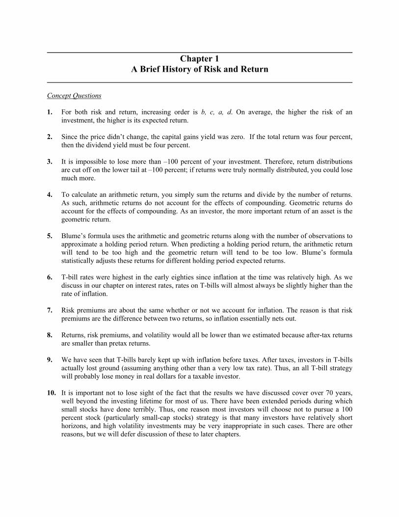
Spreadsheet Problems

Chapter 2 Buying and Selling Securities
Concept Questions 1. Purchasing on margin means borrowing some of the money used to buy securities. You do it because
you desire a larger position than you can afford to pay for, recognizing that using margin is a form of financial leverage. As such, your gains and losses will be magnified. Of course, you hope you only experience the gains.
2. Shorting a security means borrowing it and selling it, with the understanding that at some future date
you will buy the security and return it, thereby “covering” the short. You do it because you believe the security’s value will decline, so you hope to sell high now, then buy low later.
3. Margin requirements amount to security deposits. They exist to protect your broker against losses. 4. Asset allocation means choosing among broad categories such as stocks and bonds. Security
selection means picking individual assets within a particular category, such as shares of stock in particular companies.
5. They can be. Market timing amounts to active asset allocation, moving money in and out of certain
broad classes (such as stocks) in anticipation of future market direction. Of course, market timing and passive asset allocation are not the same.
6. Some benefits from street name registration include:
a. The broker holds the security, so there is no danger of theft or other loss of the security. This is
important because a stolen or lost security cannot be easily or cheaply replaced.
b. Any dividends or interest payments are automatically credited, and they are often credited more quickly (and conveniently) than they would be if you received the check in the mail.
c. The broker provides regular account statements showing the value of securities held in the
account and any payments received. Also, for tax purposes, the broker will provide all the needed information on a single form at the end of the year, greatly reducing your record-keeping requirements.
d. Street name registration will probably be required for anything other than a straight cash
purchase, so, with a margin purchase for example, it will be required. 7. Probably none. The advice you receive is unconditionally not guaranteed. If the recommendation
was grossly unsuitable or improper, then arbitration is probably your only possible means of recovery. Of course, you can close your account, or at least what’s left of it.
8. If you buy (go long) 500 shares at $18, you have a total of $9,000 invested. This is the most you can
lose because the worst that could happen is that the company could go bankrupt, leaving you with worthless shares. There is no limit to what you can make because there is no maximum value for your shares – they can increase in value without limit.
CHAPTER 2 B-7
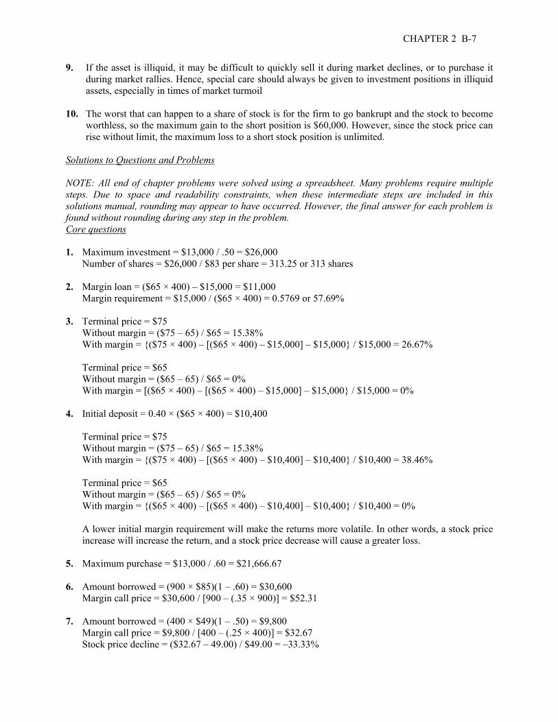
9. If the asset is illiquid, it may be difficult to quickly sell it during market declines, or to purchase it during market rallies. Hence, special care should always be given to investment positions in illiquid assets, especially in times of market turmoil
10. The worst that can happen to a share of stock is for the firm to go bankrupt and the stock to become
worthless, so the maximum gain to the short position is $60,000. However, since the stock price can rise without limit, the maximum loss to a short stock position is unlimited.
Solutions to Questions and Problems NOTE: All end of chapter problems were solved using a spreadsheet. Many problems require multiple steps. Due to space and readability constraints, when these intermediate steps are included in this solutions manual, rounding may appear to have occurred. However, the final answer for each problem is found without rounding during any step in the problem. Core questions 1. Maximum investment = $13,000 / .50 = $26,000 Number of shares = $26,000 / $83 per share = 313.25 or 313 shares 2. Margin loan = ($65 × 400) – $15,000 = $11,000 Margin requirement = $15,000 / ($65 × 400) = 0.5769 or 57.69% 3. Terminal price = $75 Without margin = ($75 – 65) / $65 = 15.38% With margin = {($75 × 400) – [($65 × 400) – $15,000] – $15,000} / $15,000 = 26.67% Terminal price = $65 Without margin = ($65 – 65) / $65 = 0% With margin = [($65 × 400) – [($65 × 400) – $15,000] – $15,000} / $15,000 = 0% 4. Initial deposit = 0.40 × ($65 × 400) = $10,400 Terminal price = $75 Without margin = ($75 – 65) / $65 = 15.38% With margin = {($75 × 400) – [($65 × 400) – $10,400] – $10,400} / $10,400 = 38.46% Terminal price = $65 Without margin = ($65 – 65) / $65 = 0% With margin = {($65 × 400) – [($65 × 400) – $10,400] – $10,400} / $10,400 = 0% A lower initial margin requirement will make the returns more volatile. In other words, a stock price
increase will increase the return, and a stock price decrease will cause a greater loss. 5. Maximum purchase = $13,000 / .60 = $21,666.67 6. Amount borrowed = (900 × $85)(1 – .60) = $30,600 Margin call price = $30,600 / [900 – (.35 × 900)] = $52.31 7. Amount borrowed = (400 × $49)(1 – .50) = $9,800 Margin call price = $9,800 / [400 – (.25 × 400)] = $32.67 Stock price decline = ($32.67 – 49.00) / $49.00 = –33.33%

B-8 SOLUTIONS
8. Proceeds from short sale = 900 × $64 = $57,600 Initial deposit = $57,600(.50) = $28,800 Account value = $57,600 + 28,800 = $86,400 Margin call price = $86,400 / [900 + (.30 × 900)] = $73.85 9. Proceeds from short sale = 1,000($56) = $56,000 Initial deposit = $56,000(.50) = $28,000 Account value = $56,000 + 28,000 = $84,000 Margin call price = $84,000 / [1,000 + (.30 × 1,000)] = $64.62 Account equity = $84,000 – (1,000 × $64.62) = $19,380 10. Pretax return = ($98.00 – 86.00 + 1.40) / $86.00 = 15.58% Aftertax capital gains = ($98.00 – 86.00)(1 – .20) = $9.60 Aftertax dividend yield = $1.40(1 – .31) = $0.966 Aftertax return = ($9.60 + .966) / $86.00 = 12.29% Intermediate questions 11. Assets Liabilities and account equity 313 shares $25,979 .00 Margin loan $12,989.50 Account equity 12,989.50 Total $25,979 .00 Total $25,979.00
Stock price = $90 Assets Liabilities and account equity 320 shares $28,170.00 Margin loan $12,989.50 Account equity 15,180.50 Total $28,170.00 Total $28,170.00
Margin = $15,180.50/$28,170 = 53.89
Stock price = $65
Assets Liabilities and account equity 320 shares $20,345.00 Margin loan $12,989.50 Account equity 7,355.50 Total $20,345.00 Total $20,345.00
Margin = $7,355.50/$20,345 = 36.15% 12. 450 shares × $41 per share = $18,450 Initial margin = $10,000/$18,450 = 54.20% Assets Liabilities and account equity 450 shares $18,450 Margin loan $8,450 Account equity 10,000 Total $18,450 Total $18,450

CHAPTER 2 B-9
13. Total purchase = 400 shares × $72 = $28,800 Margin loan = $28,800 – 15,000 = $13,800 Margin call price = $13,800 / [400 – (.30 × 400)] = $49.29
To meet a margin call, you can deposit additional cash into your trading account, liquidate shares until your margin requirement is met, or deposit additional marketable securities against your account as collateral.
14. Interest on loan = $13,800(1.065) – 13,800 = $897 a. Proceeds from sale = 400($96) = $38,400 Dollar return = $38,400 – 15,000 – 13,800 – 897 = $8,703 Rate of return = $8,703 / $15,000 = 58.02% Without margin, rate of return = ($96 – 72)/$72 = 33.33% b. Proceeds from sale = 400($72) = $28,800 Dollar return = $28,800 – 15,000 – 13,800 – 897 = –$897 Rate of return = –$897 / $15,000 = –5.98% Without margin, rate of return = $0% c. Proceeds from sale = 400($64) = $25,600 Dollar return = $25,600 – 15,000 – 13,800 – 897 = –$4,097 Rate of return = –$4,097 / $15,000 = –27.31% Without margin, rate of return = ($64 – 72) / $72 = –11.11% 15. Amount borrowed = (1,000 × $46)(1 – .50) = $23,000 Interest = $23,000 × .0870 = $2,001 Proceeds from sale = 1,000 × $53 = $53,000 Dollar return = $53,000 – 23,000 – 23,000 – 2,001 = $4,999
Rate of return = $4,999 / $23,000 = 21.73% 16. Total purchase = 800 × $32 = $25,600 Loan = $25,600 – 15,000 = $10,600 Interest = $10,600 × .083 = $879.80 Proceeds from sale = 800 × $37 = $29,600 Dividends = 800 × $.64 = $512 Dollar return = $29,600 + 512 – 15,000 – 10,600 – 879.80 = $3,632.20
Return = $3,632.20 / $15,000 = 24.21% 17. $45,000 × (1.087)6/12 – 45,000 = $1,916.68 18. $32,000 × (1.069)2/12 – 32,000 = $357.85 19. (1 + .15)12/7 – 1 = 27.07% 20. (1 + .15)12/5 – 1 = 39.85% All else the same, the shorter the holding period, the larger the EAR. 21. Holding period return = ($41 – 48 + .15) / $48 = –14.27% EAR = (1 – .1427)12/5 – 1 = –30.90%

B-10 SOLUTIONS
22. Initial purchase = 450 × $41 = $18,450 Amount borrowed = $18,450 – 10,000 = $8,450 Interest on loan = $8,450(1 + .0725)1/2 – 8,450 = $300.95 Dividends received = 450($.25) = $112.50 Proceeds from stock sale = 450($46) = $20,700 Dollar return = $20,700 + 112.50 – 10,000 – 8,450 – 300.95 = $2,061.55 Rate of return = $2,061.55 / $10,000 = 20.62 per six months Effective annual return = (1 + .2062)2 – 1 = 45.48%
23. Proceeds from sale = 2,000 × $54 = $108,000 Initial margin = $108,000 × 1.00 = $108,000 Assets Liabilities and account equity Proceeds from sale $108,000 Short position $108,000 Initial margin deposit 108,000 Account equity 108,000 Total $216,000 Total $216,000 24. Proceeds from sale = 2,000 × $54 = $108,000 Initial margin = $108,000 × .75 = $81,000 Assets Liabilities and account equity Proceeds from sale $108,000 Short position $108,000 Initial margin deposit 81,000 Account equity 81,000 Total $189,000 Total $189,000 25. Proceeds from short sale = 1,200($86) = $103,200 Initial margin deposit = $103,200(.50) = $51,600 Total assets = Total liabilities and equity = $103,200 + 51,600 = $154,800 Cost of covering short = 1,200($73) = $87,600 Account equity = $154,800 – 87,600 = $67,200 Cost of covering dividends = 1,200($1.20) = $1,440 Dollar profit = $67,200 – 51,600 – 1,440 = $14,160 Rate of return = $14,160 / $51,600 = 27.44%

CHAPTER 2 B-11
26. Proceeds from sale = 1,600 × $83 = $132,800 Initial margin = $132,800 × .50 = $66,400 Initial Balance Sheet Assets Liabilities and account equity Proceeds from sale $132,800 Short position $132,800 Initial margin deposit 66,400 Account equity 66,400 Total $199,200 Total $199,200 Stock price = $73 Assets Liabilities and account equity Proceeds from sale $132,800 Short position $116,800 Initial margin deposit 66,400 Account equity 82,400 Total $199,200 Total $199,200 Margin = $82,400 / $116,800 = 70.55% Four-month return = ($82,400 – 66,400) / $66,400 = 24.10% Effective annual return = (1 + .2410)12/5 – 1 = 67.89% Stock price = $93 Assets Liabilities and account equity Proceeds from sale $132,800 Short position $148,800 Initial margin deposit 66,400 Account equity 50,400 Total $199,200 Total $199,200 Margin = $50,400 / $148,800 = 33.87% Four-month return = ($50,400 – 66,400) / $66,400 = –24.10% Effective annual return = (1 – .2410)12/5 – 1 = –48.40%

Chapter 3 Overview of Security Types
Concept Questions 1. The two distinguishing characteristics are: (1) all money market instruments are debt instruments
(i.e., IOUs), and (2) all have less than 12 months to maturity when originally issued. 2. Preferred stockholders have a dividend preference and a liquidation preference. The dividend
preference requires that preferred stockholders be paid before common stockholders. The liquidation preference means that, in the event of liquidation, the preferred stockholders will receive a fixed face value per share before the common stockholders receive anything.
3. The PE ratio is the price per share divided by annual earnings per share (EPS). EPS is the sum of the
most recent four quarters’ earnings per share. 4. The current yield on a bond is very similar in concept to the dividend yield on common and preferred
stock 5. Volume in stocks is quoted in round lots (multiples of 100). Volume in corporate bonds is the actual
number of bonds. Volume in options is reported in contracts; each contract represents the right to buy or sell 100 shares. Volume in futures contracts is reported in contracts, where each contract represents a fixed amount of the underlying asset.
6. You make or lose money on a futures contract when the futures price changes, not the current price
for immediate delivery (although the two are closely related). 7. Open interest is the number of outstanding contracts. Since most contract positions will be closed
before maturity, it will usually shrink as maturity approaches. 8. A futures contact is a contract to buy or sell an asset at some point in the future. Both parties in the
contract are legally obligated to fulfill their side of the contract. In an option contract, the buyer has the right, but not the obligation, to buy (call) or sell (put) the asset. This option is not available to the buyer of a futures contract. The seller of a futures or options contract have the same responsibility to deliver the underlying asset. The difference is the seller of a future knows she must deliver the asset, while the seller of an option contract is uncertain about delivery since delivery is at the option purchasers discretion.
9. A real asset is a tangible asset such as a land, buildings, precious metals, knowledge, etc. A financial
asset is a legal claim on a real asset. The two basic types of financial assets are primary assets and derivative asset. A primary asset is a direct claim on a real asset. A derivative asset is basically a claim (or potential claim) in a primary asset or even another derivative asset.

CHAPTER 3 B-13
10. Initially, it might seem that the put and the call would have the same price, but this is not correct. If the strike price is exactly equal to the stock price, the call option must be worth more. Intuitively, there are two reasons. First, there is no limit to what you can make on the call, but your potential gain on the put is limited to $100 per share. Second, we generally expect that the stock price will increase, so the odds are greater that the call option will be worth something at maturity.
Core Questions 1. Dividend yield = .013 = $.30 / P0 thus P0 = $.30 / .013 = $23.08 Stock closed up $.26, so yesterday’s closing price = $23.08 – $.26 = $22.82 2,855 round lots of stock were traded. 2. PE = 16; EPS = P0 / 16 = $23.08 / 16 = $1.44 EPS = NI / shares; so NI = $1.44(25,000,000) = $36,057,692 3. Dividend yield is 3.8%, so annualized dividend is .038($84.12) = $3.20. This is just four times the
last quarterly dividend, which is thus $3.20/4 = $.80/share. 4. PE = 21; EPS = P0 / 21 = $84.12 / 21 = $4.01 5. The total par value of purchase = 4,000($1,000) = $400,000 Next payment = ($400,000 × .084) / 2 = $16,800 Payment at maturity = $16,800 + 400,000 = $416,800 Remember, the coupon payment is based on the par value of the bond, not the price. 6. Contract to buy = 700 / 50 = 14 Purchase price = 14 × 50 × $860 = $602,000 P = $895: Gain = ($895 – 860) × 14 × 50 = $24,500 P = $840: Gain = ($840 – 860) × 14 × 50 = –$14,000 7. Cost of contracts = $3.20 × 10 × 100 = $3,200 If the stock price is $78.14, the value is: ($78.14 – 70) × 10 × 100 = $8,140 Dollar return = $8,140 – 3,200 = $4,940 If the stock price is $67.56, the call is worthless, so the dollar return is –$3,200. 8. The stock is down 1.50%, so the price was $51.80/(1 – .015) = $52.59 9. Price = (126.326/100)$1,000 = $1,263.26 Current yield = Annual coupon payment / Price = $77 / $1,263.26 = 6.10% YTM of comparable Treasury = 5.768% – 1.41% = 4.358% 10. Next payment = 25(.0770/2)($1,000) = $962.50 Intermediate Questions 11. Open interest in the March contract is 64,967 contracts. Since the standard contract size is 50,000 lbs., sell 400,000/50,000 = 8 contracts. You’ll deliver 8(50,000) = 400,000 pounds of cotton and receive 8(50,000)($0.4864) = $194,560.
B-14 SOLUTIONS
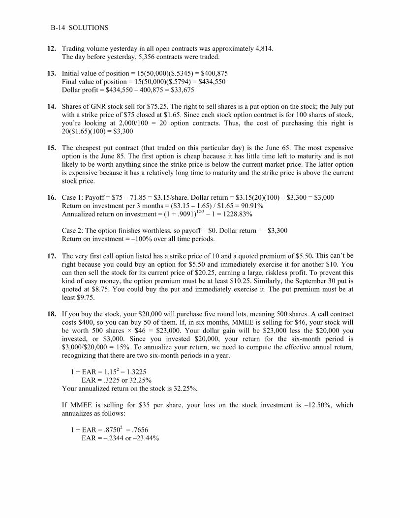
12. Trading volume yesterday in all open contracts was approximately 4,814. The day before yesterday, 5,356 contracts were traded. 13. Initial value of position = 15(50,000)($.5345) = $400,875 Final value of position = 15(50,000)($.5794) = $434,550 Dollar profit = $434,550 – 400,875 = $33,675 14. Shares of GNR stock sell for $75.25. The right to sell shares is a put option on the stock; the July put
with a strike price of $75 closed at $1.65. Since each stock option contract is for 100 shares of stock, you’re looking at 2,000/100 = 20 option contracts. Thus, the cost of purchasing this right is 20($1.65)(100) = $3,300
15. The cheapest put contract (that traded on this particular day) is the June 65. The most expensive
option is the June 85. The first option is cheap because it has little time left to maturity and is not likely to be worth anything since the strike price is below the current market price. The latter option is expensive because it has a relatively long time to maturity and the strike price is above the current stock price.
16. Case 1: Payoff = $75 – 71.85 = $3.15/share. Dollar return = $3.15(20)(100) – $3,300 = $3,000 Return on investment per 3 months = ($3.15 – 1.65) / $1.65 = 90.91% Annualized return on investment = (1 + .9091)12/3 – 1 = 1228.83% Case 2: The option finishes worthless, so payoff = $0. Dollar return = –$3,300 Return on investment = –100% over all time periods. 17. The very first call option listed has a strike price of 10 and a quoted premium of $5.50. This can’t be
right because you could buy an option for $5.50 and immediately exercise it for another $10. You can then sell the stock for its current price of $20.25, earning a large, riskless profit. To prevent this kind of easy money, the option premium must be at least $10.25. Similarly, the September 30 put is quoted at $8.75. You could buy the put and immediately exercise it. The put premium must be at least $9.75.
18. If you buy the stock, your $20,000 will purchase five round lots, meaning 500 shares. A call contract
costs $400, so you can buy 50 of them. If, in six months, MMEE is selling for $46, your stock will be worth 500 shares × $46 = $23,000. Your dollar gain will be $23,000 less the $20,000 you invested, or $3,000. Since you invested $20,000, your return for the six-month period is $3,000/$20,000 = 15%. To annualize your return, we need to compute the effective annual return, recognizing that there are two six-month periods in a year.
1 + EAR = 1.152 = 1.3225 EAR = .3225 or 32.25% Your annualized return on the stock is 32.25%. If MMEE is selling for $35 per share, your loss on the stock investment is –12.50%, which
annualizes as follows: 1 + EAR = .87502 = .7656 EAR = –.2344 or –23.44%

CHAPTER 3 B-15
At the $46 price, your call options are worth $46 – 40 = $6 each, but now you control 5,000 shares (50 contracts), so your options are worth 5,000 shares × $6 = $30,000 total. You invested $20,000, so your dollar return is $30,000 – 20,000 = $10,000, and your percentage return is $10,000/$20,000 = 50%, compared to 32.25 on the stock investment. This annualizes to:
1 + EAR = 1.502 = 2.25 EAR = 1.25 or 125% However, if MMEE is selling for $35 when your options mature, then you lose everything ($20,000
investment), and your return is –100%. 19. You only get the dividend if you own the stock. The dividend would increase the return on your
stock investment by the amount of the dividend yield, $.50/$40 = .0125, or 1.25%, but it would have no effect on your option investment. This question illustrates that an important difference between owning the stock and the option is that you only get the dividend if you own the stock.
20. At the $36.40 stock price, your put options are worth $40 – 36.40 = $3.60 each. The premium was
$2.50, so you bought 80 contracts, meaning you control 8,000 shares. Your options are worth 8,000 shares × $3.60 = $28,800 total. You invested $20,000, so your dollar return is $28,800 – 20,000 = $8,800, and your percentage return is $8,800/$20,000 = 44%. This annualizes to:
1 + EAR = 1.442 = 2.0736 EAR = 1.0736 or 107.36%

Chapter 4 Mutual Funds
Concept Questions 1. Mutual funds are owned by fund shareholders. A fund is run by the fund manager, who is hired by
the fund’s directors. The fund’s directors are elected by the shareholders. 2. A rational investor might pay a load because he or she desires a particular type of fund or fund
manager for which a no-load alternative does not exist. More generally, some investors feel you get what you pay for and are willing to pay more. Whether they are correct or not is a matter of some debate. Other investors simply are not aware of the full range of alternatives.
3. The NAV of a money market mutual fund is never supposed to change; it is supposed to stay at a
constant $1. It never rises; only in very rare instances does it fall. Maintaining a constant NAV is possible by simply increasing the number of shares as needed such that the number of shares is always equal to the total dollar value of the fund.
4. A money market deposit account is essentially a bank savings account. A money market mutual fund
is a true mutual fund. A bank deposit is insured by the FDIC, so it is safer, at least up to the maximum insured amount.
5. If your investment horizon is only one year, you probably should not invest in the fund. In this case,
the fund return has to be greater than five percent just to make back your original investment. Over a twenty-year horizon, you have more time to make up the initial load. The longer the investment horizon, the better chance you have of regaining the amount paid in a front-end load.
6. In an up market, the cash balance will reduce the overall return since the fund is partly invested in
assets with a lower return. In a down market, a cash balance should help reduce the negative returns from stocks or other instruments. An open-end fund typically keeps a cash balance to meet shareholder redemptions. A closed-end fund does not have shareholder redemptions so very little cash, if any, is kept in the portfolio.
7. 12b-1 fees are designed to pay for marketing and distribution costs. It does not really make sense that
a closed-end fund charges 12b-1 fees because there is no need to market the fund once it has been sold at the IPO and there are no distributions necessary for the fund since the shares are sold on the secondary market.
8. You should probably buy an open-end fund because the fund stands ready to buy back shares at
NAV. With a closed-end fund another buyer must make the purchase, so it may be more difficult to sell at NAV. We should note that an open-end fund may have the right to delay redemption if it so chooses.
9. Funds that accumulate a long record of poor performance tend to not attract investors. They are often
simply merged into other funds. This is a type of survivor bias, meaning that a mutual fund family’s typical long-term track record may look pretty good, but only because the poor performing funds did not survive. In fact, several hundred funds disappear each year.

CHAPTER 4 B-17
10. It doesn’t matter! For example, suppose we have a fund with a NAV of $100, a two percent fee, and a 10 percent annual return. If the fee is charged up front, we will have $98 invested, so at the end of the year, it will grow to $107.80. If the fee is charged at the end of the year, the initial investment of $100 will grow to $110. When the two percent fee is taken out, we will be left with $107.80, the same amount we would have if the fee was charged up front.
Core Questions NOTE: All end of chapter problems were solved using a spreadsheet. Many problems require multiple steps. Due to space and readability constraints, when these intermediate steps are included in this solutions manual, rounding may appear to have occurred. However, the final answer for each problem is found without rounding during any step in the problem. 1. NAV = $4,500,000,000 / 130,000,000 = $34.62 2. Load = ($36.10 – 34.62)/$36.10 = 4.11% 3. NAV = $48.65(1 – .015) = $47.92; Market value of assets = $47.92(13,400,000) = $642,128,000 4. Initial shares = 15,000. Final shares = 15,000(1.046) = 15,690, and final NAV = $1 because this is a
money market fund. 5. Total assets = (4,000 × $68) + (9,000 × $32) + (6,500 × $44) + (8,400 × $56) = $1,316,400 NAV = $1,316,400 / 50,000 = $26.33 6. NAV = ($1,316,400 – 75,000) / 50,000 = $24.83 7. Offering price = $24.83 / (1 – .05) = $26.14 8. $68,000,000 / $120,000,000 = 56.67% 9. NAV = ($350,000,000 – 800,000) / 20,000,000 = $17.46 ($15.27 – 17.46) / $17.46 = –12.54% 10. ($43.51 – 41.86 + 0.34 + 1.25) / $41.86 = 7.74% Intermediate 11. Turnover = X/$2,700,000,000 = .47; X = $1,269,000,000. This is less than the $1.45 billion in sales,
so this is the number used in the calculation of turnover in this case. 12. Management fee = .0085($2,700,000,000) = $22,950,000 Miscellaneous and administrative expenses = (.0125 – .0085)$2,700,000,000 = $10,800,000 13. Initial NAV = $41.20(1 – .05) = $39.14 Final NAV = $39.14[1 + (.12 – .0165)] = $43.19 Sale proceeds per share = $43.19(1 – .02) = $42.33 Total return = ($42.33 – 41.20) / $41.20 = 2.74% You earned 2.74% even thought the fund’s investments grew by 12%! The various fees and loads
sharply reduced your return.

B-18 SOLUTIONS
Note, there is another interpretation of the solution. To calculate the final NAV including fees, we would first find the final NAV excluding fees with a 12 percent return, which would be:
NAV excluding fees = $39.14(1 + .12) = $43.84 Now, we can find the final NAV after the fees, which would be: Final NAV = $43.84(1 – .0165) = $43.11 Notice this answer is $0.08 different than our original calculation. The reason is the assumption
behind the fee withdrawal. The second calculation assumes the fees are withdrawn entirely at the end of the year, which is generally not true. Generally, fees are withdrawn periodically throughout the year, often quarterly. The actual relationship between the return on the underlying assets, the fees charged, and the actual return earned is the same as the Fisher equation, which shows the relationship between the inflation, the nominal interest rate, and the real interest rate. In this case, we can write the relationship as:
(1 + Return on underlying assets) = (1 + Fees)(1 + Return earned) As with the Fisher equation, effective annual rates must be used. So, we would need to know the
periodic fee withdrawal and the number of fee assessments during the year to find the exact final NAV. Our first calculation is analogous to the approximation of the Fisher equation, hence it is the method of calculation we will use going forward, that is:
Return earned = Return on underlying assets – Fees Assuming a small fee (which we hope the mutual fund would have), the answer will be closest to the
actual value without undue calculations. 14. Initial NAV = $41.20; Final NAV = $41.20[1 + (.12 – .0095)] = $45.75 = Sale proceeds Total return = ($45.75 – 41.20)/$41.20 = 11.05% 15. The OTC Portfolio (“OTC”) is classified as XG, which is multi-cap growth. Its one-year return is –26.9%, which is good for a B rating. This places the fund in the top 20 to 40 percent. 16. The highest load is a substantial 8.24 percent. 17. Of the funds listed, the one with the lowest costs (in terms of expense ratios) is the “Four-in-One”
Fund. That’s a little misleading, however, because this fund actually is a “fund of funds,” meaning that it invests in other mutual funds (in this case, four of them). The highest cost funds tend to be more internationally oriented.
18. This fund has a 3% load and a NAV of $7.16. The offer price, which is what you would pay, is
$7.16/(1 – .03) = $7.38, so 1,000 shares would cost $7,380. 19. Since we are concerned with the annual return, the initial dollar investment is irrelevant, so we will
calculate the return based on a one dollar investment. 1 year: [$0.95(1 + .12)1]1/1 – 1 = 6.40% 2 years: [$0.95(1 + .12)2]1/2 – 1 = 9.16% 5 years: [$0.95(1 + .12)5]1/5 – 1 = 10.86% 10 years: [$0.95(1 + .12)10]1/10 – 1 = 11.43%

CHAPTER 4 B-19
20 years: [$0.95(1 + .12)20]1/20 – 1 = 11.71% 50 years: [$0.95(1 + .12)50]1/50 – 1 = 11.89% 20. After 3 years: (For every dollar invested) Class A: $0.9425(1 + .11 – .0023 – .0073)3 = $1.25584 Class B: [$1.00(1 + .11 – .01 – .0073)3](1 – .02) = $1.27858 After 20 years: Class A: $0.9425(1 + .11 – .0023 – .0073)20 = $6.38694 Class B: $1.00(1 + .11 – .01 – .0073)3 = $5.88869 21. (1 + .04 – .002)2 = (1 – .05)(1 + R – .0140)2; 1.07744 = 0.95(1 + R – .0140)2; R = 7.90% (1 + .04 – .002)10 = (1 – .05)(1 + R – .0140)10; 1.45202 = 0.95(1 + R – .0140)10; R = 5.73% 22. National municipal fund: after-tax yield = .039(1 – .08) = 3.59% Taxable fund: after-tax yield = .061(1 – .35 – .08) = 3.48% New Jersey municipal fund: after-tax yield = 3.60% Choose the New Jersey fund. 23. Municipal fund: after-tax yield = 3.90% Taxable fund: after-tax yield = .061(1 – .35) = 3.97% New Jersey municipal fund: after-tax yield = 3.60% Choose the taxable fund. 24. ($18.43 – NAV)/NAV = –.128; NAV = $21.14 Shares outstanding = $360M/$21.14 = 17,029,328 For closed-end funds, the total shares outstanding are fixed, just as with common stock (assuming no
net repurchases by the fund or new share issues to the public). 25. NAV at IPO = $25(1 – .08) = $23.00 (P – $23.00)/$23.00 = –.10 so P = $20.70 The value of your investment is 5,000($20.70) = $103,500, a loss of $21,500 in one day.
Chapter 5 The Stock Market
Concept Questions 1. The new car lot is a primary market; every new car sold is an IPO. The used car lot is a secondary
market. The Chevy retailer is a dealer, buying and selling out of inventory. 2. Both. When trading occurs in the crowd, the specialist acts as a broker. If necessary, the specialist
will buy or sell out of inventory to fill an order. 3. A market order is an order to execute the trade at the current market price. A limit order specifies the
highest (lowest) price at which you are willing to purchase (sell) the stock. The downside of a market order is that in a volatile market, the market price could change dramatically before your order is executed. The downside of a limit order is that the stock may never hit the limit price, meaning your trade will not be executed.
4. A stop-loss order is an order to sell at market if the price declines to the stop price. As the name
suggests, it is a tool to limit losses. As with any stop order, however, the price received may be worse than the stop price, so it may not work as well as the investor hopes. For example, suppose a stock is selling for $50. An investor has a stop loss on at $45, thereby limiting the potential loss to $5, or so the naive investor thinks. However, after the market closes, the company announces a disaster. Next morning, the stock opens at $30. The investor’s sell order will be executed, but the loss suffered will far exceed $5 per share.
5. You should submit a stop order; more specifically, a stop buy order with a stop price of $120. 6. No, you should submit a stop order to buy at $70, also called a stop buy. A limit buy would be
executed immediately at the current price. 7. With a multiple market maker system, there are, in general, multiple bid and ask prices. The inside
quotes are the best ones, the highest bid and the lowest ask. 8. What market is covered; what types of stocks are included; how many stocks are included; and how
the index is calculated. 9. The issue is index staleness. As more stocks are added, we generally start moving into less frequently
traded issues. Thus, the tradeoff is between comprehensiveness and currency. 10. The uptick rule prohibits short selling unless the last stock price change was positive, i.e. an uptick.
Until recently, it applied primarily to the NYSE, but the NASDAQ now has a similar rule. It exists to prevent “bear raids,” an illegal market manipulation involving large-scale short selling intended to force down the stock price.

CHAPTER 5 B-21
Core Questions NOTE: All end of chapter problems were solved using a spreadsheet. Many problems require multiple steps. Due to space and readability constraints, when these intermediate steps are included in this solutions manual, rounding may appear to have occurred. However, the final answer for each problem is found without rounding during any step in the problem. 1. d = (46 + 128/2 + 75) / [(45 + 128 + 75) / 3] = 2.22892 2. d = (46 + 128/3 + 75) / [(45 + 128 + 75) / 3] = 1.97189 3. a. 100 shares at $70.56 b. 100 shares at $70.53 c. 100 shares at $70.56 and 300 shares at $70.57 4. Beginning index value = (84 + 41)/2 = 62.50 Ending index value = (93 + 49)/2 = 71.00 Return = (71.00 – 62.50)/62.50 = 13.60% 5. Beginning value = [($84 × 45,000) + ($41 × 60,000)] / 2 = $3,120,000 Ending value = [($93 × 45,000) + ($49 × 60,000)] / 2 = $3,562,500 Return = ($3,562,500 – 3,120,000) / $3,120,000 = 14.18% Note you could also solve the problem as: Beginning value = ($84 × 45,000) + ($41 × 60,000) = $6,240,000 Ending value = ($93 × 45,000) + ($49 × 60,000) = $7,125,000 Return = ($7,125,000 – 6,240,000) / $6,240,000 = 14.18% The interpretation in this case is the percentage increase in the market value of the market. 6. Beginning of year: $3,210,000 / $3,120,000 × 100 = 100.00 End of year: $3,562,500 / $3,120,000 × 100 = 114.18 Note you would receive the same answer with either initial valuation method: Beginning of year: $6,240,000 / $6,240,000 × 100 = 100.00 End of year: $7,125,000 / $6,240,000 × 100 = 114.18 7. 408.16(1 + .1418) = 466.05 8. Year 1: 6,251 million / 6,251 million × 500 = 500.00 Year 2: 6,483 million / 6,251 million × 500 = 518.56 Year 3: 6,124 million / 6,251 million × 500 = 489.84 Year 4: 6,503 million / 6,251 million × 500 = 520.16 Year 2: 6,698 million / 6,251 million × 500 = 535.75 Intermediate Questions 9. d = (46/(1/3) + 128 + 75) / [(46 + 128 + 75) / 3] = 4.10843 10. Feb. 6: ∑P / 0.12560864 = 10,412.82; ∑P = 1307.94 Feb 7: ∑P = 1307.94 + 5 = 1312.94; Index level = 1312.94 / 0.12560864 = 10,452.63

B-22 SOLUTIONS
11. IBM: ∑P = 1307.94 + 80.54(.05) = 1311.967; Index level = 1311.967 / 0.12560864 = 10,444.88 Disney: ∑P = 1307.94 + 25.29(.05) = 1309.2045; Index level = 1309.2045 / 0.12560864 = 10,422.89 12. ∑P = 1307.94 + 30 = 1337.94; Index level = 1337.94 / 0.12560864 = 10,651.66 13. ∑P / d = 3,487.25; d = ∑P / 3,487.25 (∑P + 5) / d = 3,502.18; d = (∑P + 5) / 3,502.18 ∑P / 3,487.25 = (∑P + 5) / 3,502.18 3,502.18∑P = 3,487.25∑P + 17,436.25 14.93∑P = 17,436.25 ∑P = 1,167.87 1,167.87 / d = 3,487.25 d = 0.33489618 14. a. 1/1/04: Index value = (119 + 35 + 62)/3 = 72.00 b. 1/1/05: Index value = (123 + 31 + 54)/3 = 69.33 2004 return = (69.33 – 72.00)/72.00 = –3.70% 1/1/06: Index value = (132 + 39 + 68)/3 = 79.67 2005 return = (79.67 – 69.33)/69.33 = 14.90% 15. Share price after the stock split is $41. Index value on 1/1/05 without the split is 69.33 (see above). (41 + 31 + 54)/d = 69.33; d = 126 / 69.33 = 1.8317308 1/1/06: Index value = (44 + 39 + 68)/1.8317308 = 83.0899 2005 return = (83.0899 – 69.33)/69.33 = 19.84%. Notice without the split the index return for 2004 is 14.90%. 16. a. 1/1/04: Index value = [119(220) + 35(400) + 62(350)] / 10 = 6188.00 b. 1/1/05: Index value = [123(220) + 31(400) + 54(350)] / 10 = 5836.00 2004 return = (5836 – 6188) / 6188 = –5.69% 1/1/06: Index value = [132(220) + 39(400) + 68(350)] /10 = 6844.00 2005 return = (6844 – 5836) / 5836 = 17.27% 17. The index values and returns will be unchanged; the stock split changes the share price, but not the
total value of the firm.
CHAPTER 5 B-23
18. 2004: Douglas McDonnell return = (123 – 119)/119 = 3.36% Dynamics General return = (31 – 35)/35 = –11.43% International Rockwell return = (54 – 62)/62 = –12.90% 2004: Index return = (.0336 – .1143 – .1290)/3 = –6.99% 1/1/05: Index value = 100(1 – .0699) = 93.01 2005: Douglas McDonnell return = (132 – 123)/123 = 7.32% Dynamics General return = (39 – 31)/31 = 25.81% International Rockwell return = (68 – 54)/54 = 25.93% 2005: Index return = (.0732 + .2581 + .2593)/3 = 19.68% 1/1/06: Index value = 93.01(1.1968) = 111.32 19. Looking back at Chapter 1, you can see that there are years in which small cap stocks outperform
large cap stocks. In years with better performance by small companies, we would expect the returns from the equal-weighted index to outperform the value-weighted index since the value-weighted index is weighted toward larger companies. In years where large cap stocks outperform small cap stocks, we would see the value-weighted index with a higher return than an equal-weighted index.
20. 2004: Douglas McDonnell return = (123 – 119)/119 = 3.36% Dynamics General return = (31 – 35)/35 = –11.43% International Rockwell return = (54 – 62)/62 = –12.90% 2004: Index return = [(1 + .0336)(1 – .1143)(1 – .1290)]1/3 – 1 = –7.27% 1/1/05: Index value = 100(1 – .0727) = 92.73 2005: Douglas McDonnell return = (132 – 123)/123 = 7.32% Dynamics General return = (39 – 31)/31 = 25.81% International Rockwell return = (68 – 54)/54 = 25.93% 2005: Index return = [(1 + .0732)(1 + .2851)(1 + .2593)]1/3 – 1 = 19.35% 1/1/06: Index value = 92.73(1.1935) = 110.67 21. A geometric index is most suitable to capture the short-term price movements of the stocks in the
index, but is not suitable for long-term investment performance measurement. A geometric index is an attempt to capture the median stock return. There are two reasons for the difference in the index levels. First, the geometric index systematically understates performance. The second reason is volatility. The geometric index, by its construction, filters out volatility. On the other hand, an equal-weighted index tends to capture market upswings.

B-24 SOLUTIONS
22. For price-weighted indices, purchase an equal number of shares for each firm in the index. For value- weighted indices, purchase shares (perhaps in fractional amounts) so that the investment in each stock, relative to your total portfolio value, is equal to that stock’s proportional market value relative to all firms in the index. In other words, if one company is twice as big as the other, put twice as much money in that company. Finally, for equally-weighted indices, purchase equal dollar amounts of each stock in the index.
Assuming no cash dividends or stock splits, both the price-weighted and value-weighted replication strategies require no additional rebalancing. However, an equally weighted index will not stay equally weighted through time, so it will have to be rebalanced by selling off investments that have gone up in value and buying investments that have gone down in value.
A typical small investor would most likely use something like the equally-weighted index replication strategy, i.e., buying more-or-less equal dollar amounts of a basket of stocks, but the portfolio probably would not stay equally weighted. The value-weighted and equally-weighted index replication strategies are more difficult to implement than the price-weighted strategy because they would likely involve the purchase of odd lots and fractional shares, raising transactions costs. The value-weighted strategy is the most difficult because of the extra computation needed to determine the initial amounts to invest.

Chapter 6 Common Stock Valuation
Concept Questions 1. The basic principle is that we can value a share of stock by computing the present value of all future
dividends. 2. P/E ratios measure the price of a share of stock relative to current earnings. All else the same, future
earnings will be larger for a growth stock than a value stock, so investors will pay more relative to today’s earnings.
3. As you know, firms can have negative earnings. But, for a firm to survive over a long period,
earnings must eventually become positive. The residual income model will give a negative stock value when earnings are negative, thus it cannot be used reliably in this situation.
4. It is computed by taking net income plus depreciation and then dividing by the number of shares
outstanding. 5. The value of any investment depends on its cash flows; i.e., what investors will actually receive. The
cash flows from a share of stock are the dividends. 6. Investors believe the company will eventually start paying dividends (or be sold to another company). 7. In general, companies that need the cash will often forgo dividends since dividends are a cash
expense. Young, growing companies with profitable investment opportunities are one example; another example is a company in financial distress.
8. The general method for valuing a share of stock is to find the present value of all expected future
dividends. The constant perpetual growth model presented in the text is only valid (i) if dividends are expected to occur forever, that is, the stock provides dividends in perpetuity, and (ii) if a constant growth rate of dividends occurs forever. A violation of the first assumption might be a company that is expected to cease operations and dissolve itself some finite number of years from now. The stock of such a company would be valued by the methods of this chapter by applying the general method of valuation. A violation of the second assumption might be a start-up firm that isn’t currently paying any dividends, but is expected to eventually start making dividend payments some number of years from now. This stock would also be valued by the general dividend valuation method of this chapter.
9. The two components are the dividend yield and the capital gains yield. For most companies, the
capital gains yield is larger. This is easy to see for companies that pay no dividends. For companies that do pay dividends, the dividend yields are rarely over five percent and are often much less.
10. Yes. If the dividend grows at a steady rate, so does the stock price. In other words, the dividend
growth rate and the capital gains yield are the same.

B-26 SOLUTIONS
Solutions to Questions and Problems NOTE: All end of chapter problems were solved using a spreadsheet. Many problems require multiple steps. Due to space and readability constraints, when these intermediate steps are included in this solutions manual, rounding may appear to have occurred. However, the final answer for each problem is found without rounding during any step in the problem. Core Questions 1. V(0) = $3.25/(1.11)1 + $3.25/(1.11)2 + $3.25/(1.11)3 + $3.25/(1 + .11)4 + $50/(1.11)4 = $43.02 2. V(0) = $3.25/(1.11)1 + $3.25/(1.11)2 + $3.25/(1.11)3 + $3.25/(1 + .11)4 + $LD/(1.11)4 = $50.00 $39.92 = LD/(1 + .11)4 LD = $60.60 3. V(0) = [$2(1.06)/(.12 – .06)][1 – (1.06/1.12)5] = $8.50 V(0) = [$2(1.06)/(.12 – .06)][1 – (1.06/1.12)10] = $14.96 V(0) = [$2(1.06)/(.12 – .06)][1 – (1.06/1.12)30] = $28.56 V(0) = [$2(1.06)/(.12 – .06)][1 – (1.06/1.12)100] = $35.19 4. V(0) = $30 = [D(1.07)/(.14 – .07)][1 – (1.07/1.14)10] ; D = $4.18 5. V(0) = [$4.00(1.20)/(.10 – .20)][1 – (1.20/1.10)25] = $374.63 V(0) = [$4.00(1.12)/(.10 – .12)][1 – (1.12/1.10)25] = $127.46 V(0) = [$4.00(1.06)/(.10 – .06)][1 – (1.06/1.10)25] = $64.01 V(0) = [$4.00(1.00)/(.10 – .00)][1 – (1.00/1.10)25] = $36.31 V(0) = [$4.00(0.95)/(.10 + .05)][1 – (0.95/1.10)25] = $24.68 6. V(0) = [$1.80(1.062)]/(.1180 – .0620) = $34.14 7. V(0) = $60 = $4.10/(k – .04) , k = .04 + 4.10/60 = 10.833% 8. V(0) = $35 = [$1.80(1+g)]/(.12 – g) ; g = 6.52% 9. V(0) = $48 = D(1)/(.09 – .045) ; D(1) = $2.16 D(3) = $2.16(1.045)2 = $2.36 10. Retention ratio = 1 – ($0.75/$2.20) = .6591 Sustainable growth rate = .18(.6591) = 11.86% 11. Sustainable growth = .06 = .17r ; retention ratio = .3529 Payout ratio = 1 – .3529 = .6471 = D/EPS = $1.40/EPS ; EPS = $1.40/.6471 = $2.16 P/E = 23, EPS = $2.16, so V(0) = $2.16(23) = $49.76 12. E(R) = .045 + .70(.085) = .1045 or 10.45% E(R) = .045 + 1.25(.085) = .1513 or 15.13% 13. P0 = $4.50 + [$5.00 – ($4.50 × .012)]/(0.12 – 0.04) = $60.25 14. P0 = $4.50 + [($5.00 × 1.04) – ($4.50 × .012)]/(0.12 – 0.04) = $67.25

CHAPTER 6 B-27
Intermediate Questions 15. V(0) = [$1.45(1.25)/(.14 – .25)][1 – (1.25/1.14)8] + [(1 + .25)/(1 + .14)]8[$1.45(1.07)/(.14 – .07)] = $64.26 16. V(0) = [$1.34(1.21)/(.12 – .21)][1 – (1.21/1.12)12] + [(1 + .21)/(1 + .12)]12[$1.34(1.06)/(.12 – .06)] = $87.38 17. V(9) = D(10)/(k – g) = $5/(.15 – .07) = $62.50 V(0) = V(9)/(1.15)9 = $62.50/(1.15)9 = $17.77 18. D(3) = D(0)(1.25)3 ; D(4) = D(0)(1.25)3(1.2) V(4) = D(4)(1 + g)/(k–g) = D(0)(1.25)3(1.2)(1.07)/(.13–.07) = 41.7696D(0) V(0) = $62.10 = D(0){ (1.25/1.13) + (1.25/1.13)2 + (1.25/1.13)3 + [1.353(1.2) + 41.7696]/1.144 } D(0) = $62.10/$30.756 = $2.02 ; D(1) = $2.02(1.25) = $2.52 19. V(4) = $1.50(1.07)/(.14 – .07) = $22.93 V(0) = $9.00/1.14 + $11.00/1.142 + $7.00/1.143 + ($1.50 + 22.93)/1.144 = $35.55 20. V(6) = D(7)/(k – g) = $3.50(1.065)7/(.11 – .065) = $120.87 V(3) = $3.50(1.065)4/1.14 + $3.50(1.065)5/1.142 + $3.50(1.065)6/1.143 + $120.87/1.143 = $92.67 V(0) = $3.50(1.065)/1.19 + $3.50(1.065)2/1.192 + $3.50(1.065)3/1.193 + $92.67/1.193 = $63.43 21. P/E ratio: values are: 25.10, 26.26, 27.50, 30.69, 25.29, 28.20 ; average = 27.34 EPS growth rates: 5.88%, 3.70%, 3.57%, 17.24%, 10.29% ; average = 8.14% Expected share price using P/E = 27.34($3.75)(1.0814) = $110.87 P/CFPS: values are: 12.31, 12.52, 12.58, 13.63, 12.74, 15.13 ; average = 13.15 CFPS growth rates = 10.58%; 6.43%, 6.70%, 3.73%, 5.78% ; average = 6.57% Expected share price using P/CFPS= 13.15($7.14)(1.0657) = $100.07 P/S: values are: 1.362, 1.417, 1.389, 1.477, 1.324, 1.592 ; average = 1.427 SPS growth rates: 8.09%, 9.11%, 8.73%, 7.78%, 4.45% ; average = 7.63% Expected share price = 1.427($67.85)(1.0763) = $104.19 A reasonable price range would seem to be $100 to $111 per share. 22. k = .05 + 0.85(.085) = 12.23% Dividend growth rates: 7.27%, 7.63%, 5.51%, 4.48%, 7.14% ; average = 6.41% V(2005) = $1.50(1.0641)2 / (.1223 – .0641) = $29.19 Notice the last dividend is for 2005. To find the price in 2006, we must use the dividend in 2007 in
the constant perpetual dividend growth model.

B-28 SOLUTIONS
23. P/E ratio: N/A, N/A, N/A, 12,400, 3,366.67, 180.00 ; average = 1,773.33 EPS growth rates: 46.67%, 34.38%, 33.335%, 102.14%, 66.67% ; average = 56.64% Expected share price using P/E = 1,773.33($0.05)(1.5664) = $138.88 P/CFPS: N/A, N/A, N/A, N/A, 2,520.00, 112.50 ; average = 1,318.75 CFPS growth rates: 35.00%, 50.00%, 67.31%, 104.71%, 100.00% ; average = 71.40% Expected share price using P/CFPS = 1,318.75($0.09)(1.7140) = $180.83 P/S: values are 2.250, 4.077, 8.412, 10.722, 4.927, 0.516 ; average = 5.150 SPS growth rates: 62.50%, 30.77%, 14.12%, 5.67%, –14.88% ; average = 19.64% Expected share price using P/S = 5.150($17.45)(1.1964) = $107.52 This price range is from $107 to $181! As long as the stellar growth continues, the stock should do
well. But any stumble will likely tank the stock. Be careful out there! 24. P/E ratios and P/CFPS are all negative, so these ratios are unusable. P/S: values are 25.867, 6.063, 1.127 ; average = 11.019 SPS growth rates = 91.22%, 43.66% ; average = 70.44% Expected share price using SPS = 11.019($10.20)(1.7044) = $191.57 This price is ridiculous, $192! Notice that sales have been exploding, but the company still can’t
make money. The market price of $11.50 might be fair considering the risks involved. Might be a buyout candidate, but at what price?
25. Parador’s expected future stock price is $70 × 1.14 = $79.80, and expected future earnings per share
is $4.50 × 1.08 = $4.89. Thus, Parador’s expected future P/E ratio is $79.80 / $4.86 = 16.42. 26. Parador’s expected future stock price is $70 × 1.14 = $79.80, and expected future sales per share is
$23 × 1.09 = $25.07. Thus, Parador’s expected future P/E ratio is $79.80 / $25.07 = 3.183. 27. b = 1 – ($1.10 / $2.50) = .56; g = 26.50% × .56 = 14.84% k = 3.79% + 0.85(8%) = 10.59% P0 = $1.10(1 + .0840) / (.1059 – .1584) = –$29.72 Since the growth rate is higher than required return, the dividend growth model cannot be used. 28. Average stock price: $49.60, $43.90, $40.50, $42.95, $44.050 P/E ratio: 26.38, 21.31, 18.33, 18.92, 17.62; Average P/E = 20.51 EPS growth rates: 9.57%, 7.28%, 2.71%, 10.13%; Average EPS growth = 7.43% P/E price: 20.51(1.0743)($2.50) = $55.09 P/CF ratio: 18.72, 15.51, 13.46, 14.08, 12.96; Average P/CF = 14.94 CF growth rates: 6.79%, 6.36%, 1.33%, 11.48%, Average CF growth rate = 6.49% P/CF price = 14.94(1.0649)($3.40) = $54.11 P/S ratios: 4.733, 3.882, 3.253, 3.439, 3.048; Average P/S = 3.671 SPS growth rates: 7.92%, 10.08%, 0.32%, 15.69%; Average SPS growth rate = 8.50% P/S price = 3.671(1.0850)($14.45) = $57.56 29. EPS next year = $2.50(1.0840) = $2.71 Book value next year = $9.50(1.0840) = $10.30 V(0) = $9.50 + [$2.71 – ($9.50 × .1059)]/(0.1059 – 0.0840) = $87.31 30. Clean dividend = $2.71 – ($10.30 – 9.50) = $1.91 V(0) = $1.91 / (.1059 – .1484) = –$34.38

CHAPTER 6 B-29
31. Based on price ratio analysis, it appears the stock should be priced around $55. All three ratios give remarkably consistent prices for Abbott. The constant perpetual growth model and RIM model cannot be used because the growth rate is greater than the required return.
32. The values for the end of the year are: Book value = $10.85(1.1250) = $12.21 EPS = $2.88(1.11) = $3.20 Note, to find the book value in the first year, we can use the following relationship: B2 – B1 = B1(1 + g) – B1 = B1 + B1g – B1 = B1g We will use this relationship to calculate the book value in the following years, so:
V(0) = 1.082
10.85) - ($12.21 - $3.20 + 21.082.1250) ($12.21 - 1.11) ($3.20 ××
+ 3
2
1.082.1250) 1.125 ($12.21 - )1.11 ($3.20 ××× + 4
23
1.082.1250) 1.125 ($12.21 - )1.11 ($3.20 ×××
+ 4
3
1.0821.1250 $12.21× + 4
33
1.082.06) - 820.0820)/(.0 1.1250 ($12.21 - 1.06) 1.11 ($3.20 ××××
V(0) = $126.08 33. ROE = Net income / Equity = $80 / $674 = 11.87%; Retention ratio = 1 – $24 / $80 = .70 Sustainable growth = 11.87%(.30) = 8.3086% 34. An increase in the quarterly dividend will decrease the growth rate as it will lower the retention ratio.
A stock split affects none of the components, therefore will have no effect. 35. V(0) = [$0.286(1.32)/(.13 – .32)][1 – (1.32/1.14)2] + [(1 + .32)/(1 + .13)]2[$0.286(1.14)/(.14 – .13)] V(0) = $44.04 36. P/E on next year’s earnings = .30 / (.14 – .13) = 30.00 37. Using the following relationships: P0 = D1 / k – g; DPS1 = EPS1(1 – b); g = ROE× b; k = Rf + β(MRP) The P/E ratio can be re-written as: P/E = (1 – b) / {[Rf +β(MRP)] – (ROE × b)} a. As the beta increases, the P/E ratio should decrease. The required return increases, decreasing the present value of the future dividends. b. As the growth rate increases, the P/E ratio increases. c. An increase in the payout ratio would increase the P/E ratio. Although b is in the numerator and the denominator, the effect is greater in the denominator d. As the market risk premium increases, the P/E ratio decreases. The required return increases, decreasing the present value of the future dividends. 38. Signaling theory can explain the paradox. If investors believe that the increased dividend is a signal of
no potential growth opportunities for the company, investors may re-evaluate the expected growth rate of the company. A lower growth rate could offset the higher dividend. It is also possible that investors believe the company does have potential growth opportunities, but is not exploiting them. In this case, the growth rate of the company would also be lowered.

Chapter 7 Stock Price Behavior and Market Efficiency
Concept Questions 1. The market is not weak-form efficient. 2. Unlike gambling, the stock market is a positive sum game; everybody can win. Also, speculators
provide liquidity to markets and thus help promote efficiency. 3. The efficient markets paradigm only says, within the bounds of increasingly strong assumptions about
the information processing of investors, that assets are fairly priced. An implication of this is that, on average, the typical market participant cannot earn excess profits from a particular trading strategy. However, that does not mean that a few particular investors cannot outperform the market over a particular investment horizon. Certain investors who do well for a period of time get a lot of attention from the financial press, but the scores of investors who do not do well over the same period of time generally get considerably less attention.
4. a. If the market is not weak-form efficient, then this information could be acted on and a profit
earned from following the price trend. Under 2, 3, and 4, this information is fully impounded in the current price and no abnormal profit opportunity exists.
b. Under 2, if the market is not semistrong form efficient, then this information could be used to buy the stock “cheap” before the rest of the market discovers the financial statement anomaly. Since 2 is stronger than 1, both imply a profit opportunity exists; under 3 and 4, this information is fully impounded in the current price and no profit opportunity exists.
c. Under 3, if the market is not strong form efficient, then this information could be used as a
profitable trading strategy, by noting the buying activity of the insiders as a signal that the stock is underpriced or that good news is imminent. Since 1 and 2 are weaker than 3, all three imply a profit opportunity. Under 4, the information doesn’t signal a profit opportunity for traders; pertinent information the manager-insiders may have is fully reflected in the current share price.
d. Despite the fact that this information is obviously less open to the public and a clearer signal of
imminent price gains than is the scenario in part (c), the conclusions remain the same. If the market is strong form efficient, a profit opportunity does not exist. A scenario such as this one is the most obvious evidence against strong-form market efficiency; the fact that such insider trading is also illegal should convince you of this fact.
5. Taken at face value, this fact suggests that markets have become more efficient. The increasing ease
with which information is available over the internet lends strength to this conclusion. On the other hand, during this particular period, large-cap growth stocks were the top performers. Value-weighted indexes such as the S&P 500 are naturally concentrated in such stocks, thus making them especially hard to beat during this period. So, it may be that the dismal record compiled by the pros is just a matter of bad luck or benchmark error.

CHAPTER 7 B-31
6. It is likely the market has a better estimate of the stock price, assuming it is semistrong form efficient. However, semistrong form efficiency only states that you cannot easily profit from publicly available information. If financial statements are not available, the market can still price stocks based upon the available public information, limited though it may be. Therefore, it may have been as difficult to examine the limited public information and make an extra return.
7. Beating the market during any year is entirely possible. If you are able to consistently beat the market,
it may shed doubt on market efficiency unless you are taking more risk than the market as a whole or are simply lucky.
8. a. False. Market efficiency implies that prices reflect all available information, but it does not
imply certain knowledge. Many pieces of information that are available and reflected in prices are fairly uncertain. Efficiency of markets does not eliminate that uncertainty and therefore does not imply perfect forecasting ability.
b. True. Market efficiency exists when prices reflect all available information. To be efficient in
the weak form, the market must incorporate all historical data into prices. Under the semi-strong form of the hypothesis, the market incorporates all publicly-available information in addition to the historical data. In strong form efficient markets, prices reflect all publicly and privately available information.
c. False. Market efficiency implies that market participants are rational. Rational people will
immediately act upon new information and will bid prices up or down to reflect that information.
d. False. In efficient markets, prices reflect all available information. Thus, prices will fluctuate
whenever new information becomes available. e. True. Competition among investors results in the rapid transmission of new market
information. In efficient markets, prices immediately reflect new information as investors bid the stock price up or down.
9. Yes, historical information is also public information; weak form efficiency is a subset of semi-strong
form efficiency. 10. Ignoring trading costs, on average, such investors merely earn what the market offers; the trades all
have zero NPV. If trading costs exist, then these investors lose by the amount of the costs. 11. a. Aerotech’s stock price should rise immediately after the announcement of the positive news. b. Only scenario (ii) indicates market efficiency. In that case, the price of the stock rises
immediately to the level that reflects the new information, eliminating all possibility of abnormal returns. In the other two scenarios, there are periods of time during which an investor could trade on the information and earn abnormal returns.
12. False. The stock price would have adjusted before the founder’s death only if investors had perfect
forecasting ability. The 12.5 percent increase in the stock price after the founder’s death indicates that either the market did not anticipate the death or that the market had anticipated it imperfectly. However, the market reacted immediately to the new information, implying efficiency. It is interesting that the stock price rose after the announcement of the founder’s death. This price behavior indicates that the market felt he was a liability to the firm.

B-32 SOLUTIONS
13. The announcement should not deter investors from buying UPC’s stock. If the market is semi-strong form efficient, the stock price will have already reflected the present value of the payments that UPC must make. The expected return after the announcement should still be equal to the expected return before the announcement. UPC’s current stockholders bear the burden of the loss, since the stock price falls on the announcement. After the announcement, the expected return moves back to its original level.
14. The market is generally considered to be efficient up to the semi-strong form. Therefore, no
systematic profit can be made by trading on publicly-available information. Although illegal, the lead engineer of the device can profit from purchasing the firm’s stock before the news release on the implementation of the new technology. The price should immediately and fully adjust to the new information in the article. Thus, no abnormal return can be expected from purchasing after the publication of the article.
15. Under the semi-strong form of market efficiency, the stock price should stay the same. The
accounting system changes are publicly available information. Investors would identify no changes in either the firm’s current or its future cash flows. Thus, the stock price will not change after the announcement of increased earnings.
16. Because the number of subscribers has increased dramatically, the time it takes for information in the
newsletter to be reflected in prices has shortened. With shorter adjustment periods, it becomes impossible to earn abnormal returns with the information provided by Durkin. If Durkin is using only publicly-available information in its newsletter, its ability to pick stocks is inconsistent with the efficient markets hypothesis. Under the semi-strong form of market efficiency, all publicly-available information should be reflected in stock prices. The use of private information for trading purposes is illegal.
17. You should not agree with your broker. The performance ratings of the small manufacturing firms
were published and became public information. Prices should adjust immediately to the information, thus preventing future abnormal returns.
18. Stock prices should immediately and fully rise to reflect the announcement. Thus, one cannot expect
abnormal returns following the announcement. 19. a. No. Earnings information is in the public domain and reflected in the current stock price. b. Possibly. If the rumors were publicly disseminated, the prices would have already adjusted for
the possibility of a merger. If the rumor is information that you received from an insider, you could earn excess returns, although trading on that information is illegal.
c. No. The information is already public, and thus, already reflected in the stock price. 20. The statement is false because every investor has a different risk preference. Although the expected
return from every well-diversified portfolio is the same after adjusting for risk, investors still need to choose funds that are consistent with their particular risk level.
21. The share price will decrease immediately to reflect the new information. At the time of the
announcement, the price of the stock should immediately decrease to reflect the negative information.
CHAPTER 7 B-33
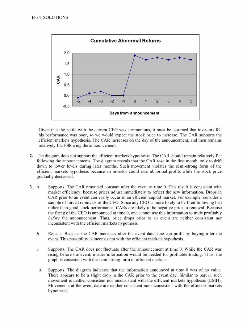
22. In an efficient market, the cumulative abnormal return (CAR) for Prospectors would rise substantially at the announcement of a new discovery. The CAR falls slightly on any day when no discovery is announced. There is a small positive probability that there will be a discovery on any given day. If there is no discovery on a particular day, the price should fall slightly because the good event did not occur. The substantial price increases on the rare days of discovery should balance the small declines on the other days, leaving CARs that are horizontal over time. The substantial price increases on the rare days of discovery should balance the small declines on all the other days, leavings CARs that are horizontal over time.
Solutions to Questions and Problems NOTE: All end of chapter problems were solved using a spreadsheet. Many problems require multiple steps. Due to space and readability constraints, when these intermediate steps are included in this solutions manual, rounding may appear to have occurred. However, the final answer for each problem is found without rounding during any step in the problem. Core Questions 1. To find the cumulative abnormal returns, we chart the abnormal returns for the days preceding and
following the announcement. The abnormal return is calculated by subtracting the market return from the stock’s return on a particular day, Ri – RM. Calculate the cumulative average abnormal return by adding each abnormal return to the previous day’s abnormal return.
Daily Cumulative Days from Abnormal Abnormal Announcement Return Return -5 -0.1 -0.1 -4 0.2 0.1 -3 0.1 0.2 -2 -0.2 0.0 -1 0.0 0.0 0 1.9 1.9 1 -0.2 1.7 2 0.1 1.8 3 -0.1 1.7 4 0.1 1.8 5 -0.1 1.7
B-34 SOLUTIONS
Cumulative Abnormal Returns
-0.5
0.0
0.5
1.0
1.5
2.0
-5 -4 -3 -2 -1 0 1 2 3 4 5
Days from announcement
CAR
Given that the battle with the current CEO was acrimonious, it must be assumed that investors felt
his performance was poor, so we would expect the stock price to increase. The CAR supports the efficient markets hypothesis. The CAR increases on the day of the announcement, and then remains relatively flat following the announcement.
2. The diagram does not support the efficient markets hypothesis. The CAR should remain relatively flat
following the announcements. The diagram reveals that the CAR rose in the first month, only to drift down to lower levels during later months. Such movement violates the semi-strong form of the efficient markets hypothesis because an investor could earn abnormal profits while the stock price gradually decreased.
3. a. Supports. The CAR remained constant after the event at time 0. This result is consistent with
market efficiency, because prices adjust immediately to reflect the new information. Drops in CAR prior to an event can easily occur in an efficient capital market. For example, consider a sample of forced removals of the CEO. Since any CEO is more likely to be fired following bad rather than good stock performance, CARs are likely to be negative prior to removal. Because the firing of the CEO is announced at time 0, one cannot use this information to trade profitably before the announcement. Thus, price drops prior to an event are neither consistent nor inconsistent with the efficient markets hypothesis.
b. Rejects. Because the CAR increases after the event date, one can profit by buying after the
event. This possibility is inconsistent with the efficient markets hypothesis. c. Supports. The CAR does not fluctuate after the announcement at time 0. While the CAR was
rising before the event, insider information would be needed for profitable trading. Thus, the graph is consistent with the semi-strong form of efficient markets.
d. Supports. The diagram indicates that the information announced at time 0 was of no value.
There appears to be a slight drop in the CAR prior to the event day. Similar to part a, such movement is neither consistent nor inconsistent with the efficient markets hypothesis (EMH). Movements at the event date are neither consistent nor inconsistent with the efficient markets hypothesis.

CHAPTER 7 B-35
4. Once the verdict is reached, the diagram shows that the CAR continues to decline after the court decision, allowing investors to earn abnormal returns. The CAR should remain constant on average, even if an appeal is in progress, because no new information about the company is being revealed. Thus, the diagram is not consistent with the efficient markets hypothesis (EMH).
Intermediate Questions 5. To find the cumulative abnormal returns, we chart the abnormal returns for each of the three
companies for the days preceding and following the announcement. The abnormal return is calculated by subtracting the market return from a stock’s return on a particular day, Ri – RM. Group the returns by the number of days before or after the announcement for each respective company. Calculate the cumulative average abnormal return by adding each abnormal return to the previous day’s abnormal return.
Abnormal returns (Ri – RM)
Days from announcement
Ross
W’field
Jaffe
Sum
Average abnormal return
Cumulative average residual
–4 –0.2 –0.2 –0.2 –0.6 –0.2 –0.2–3 0.2 –0.1 0.2 0.3 0.1 –0.1–2 0.2 –0.2 0.0 0.0 0.0 –0.1–1 0.2 0.2 –0.4 0.0 0.0 –0.1
0 3.3 0.2 1.9 5.4 1.8 1.71 0.2 0.1 0.0 0.3 0.1 1.82 –0.1 0.0 0.1 0.0 0.0 1.83 –0.2 0.1 –0.2 –0.3 –0.1 1.74 –0.1 –0.1 –0.1 –0.3 –0.1 1.6
Cumulative Abnormal Returns
-0.5
0.0
0.5
1.0
1.5
2.0
-4 -3 -2 -1 0 1 2 3 4
Days from announcement
CAR
The market reacts favorably to the announcements. Moreover, the market reacts only on the day of
the announcement. Before and after the event, the cumulative abnormal returns are relatively flat. This behavior is consistent with market efficiency.

Chapter 8 Behavioral Finance and the Psychology of Investing
Concept Questions 1. There are three trends at all times, the primary, secondary, and tertiary trends. For a market timer, the
secondary, or short-run trend, might be the most important, but, for most investors, it is the primary, or long-run trend that matters.
2. A support area is a price or level below which a stock price or market index is not likely to drop. A
resistance area is a price or level above which a stock price or market index is not likely to rise. 3. A correction is movement toward the long-run trend. A confirmation is a signal that the long-run
trend has changed direction. 4. The fact that the market is up is good news, but market breadth (the difference between the number of
gainers and losers) is negative. To a technical analyst, a market advance on narrow or negative breadth is not a particularly positive event.
5. The Arms (or trin) is a ratio. The numerator has the average number of shares traded in stocks that
were down for the day; the denominator has the average number of shares traded that were up for the day. It indicates whether trading is heavier in down or up issues.
6. If the market is efficient, then market timing is a bad idea. Trying to time the market will only mean
that over a long period, the investor will underperform a strategy that stays fully invested. A timing strategy will incur significant costs and, likely, taxes as well.
7. At the time the theory was developed, large companies in the U.S. were either involved in the
manufacturing of goods or the transportation of them (primarily railroads). The basic idea behind the Dow theory is that these activities are fundamentally related, so the two averages must move in the same direction over time.
8. The least likely limit to arbitrage is firm-specific risk. For example, in the 3Com/Palm case, the stocks
are perfect substitutes after accounting for the exchange ratio. An investor could invest in a risk neutral portfolio by purchasing the underpriced asset and selling the overpriced asset. When the prices of the assets revert to an equilibrium, the positions could be closed.
9. A contrarian investor goes against the crowd. For example, when investors are bullish, a contrarian
would argue the market is overbought and short sell. Conversely, when investors are pessimistic, a contrarian would begin purchasing stocks.
10. Consider support and resistance lines. If it is agreed the resistance line is $90, what would a rational
investor do when the stock price reaches $89 (or some other suitable close price)? The investor would sell the stock. This means the new resistance line is $89. Now, an investor would sell at $88. This logic implies the support and resistance lines would collapse on each other.
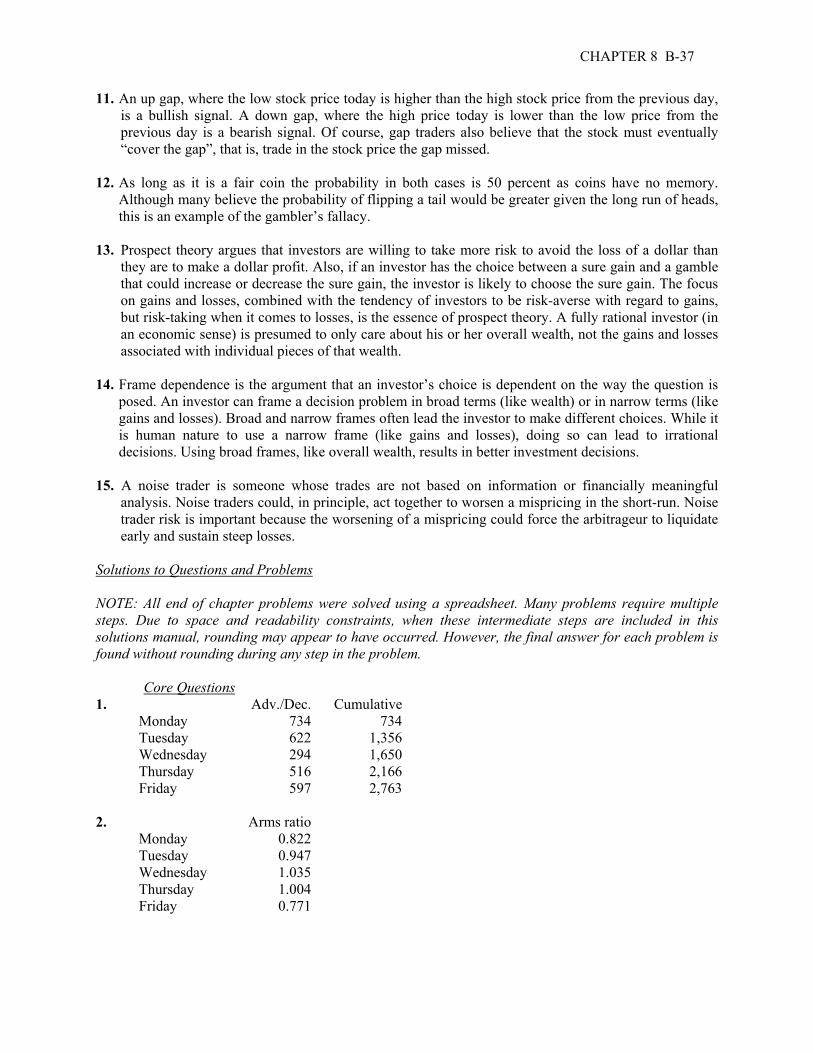
CHAPTER 8 B-37
11. An up gap, where the low stock price today is higher than the high stock price from the previous day, is a bullish signal. A down gap, where the high price today is lower than the low price from the previous day is a bearish signal. Of course, gap traders also believe that the stock must eventually “cover the gap”, that is, trade in the stock price the gap missed.
12. As long as it is a fair coin the probability in both cases is 50 percent as coins have no memory.
Although many believe the probability of flipping a tail would be greater given the long run of heads, this is an example of the gambler’s fallacy.
13. Prospect theory argues that investors are willing to take more risk to avoid the loss of a dollar than
they are to make a dollar profit. Also, if an investor has the choice between a sure gain and a gamble that could increase or decrease the sure gain, the investor is likely to choose the sure gain. The focus on gains and losses, combined with the tendency of investors to be risk-averse with regard to gains, but risk-taking when it comes to losses, is the essence of prospect theory. A fully rational investor (in an economic sense) is presumed to only care about his or her overall wealth, not the gains and losses associated with individual pieces of that wealth.
14. Frame dependence is the argument that an investor’s choice is dependent on the way the question is
posed. An investor can frame a decision problem in broad terms (like wealth) or in narrow terms (like gains and losses). Broad and narrow frames often lead the investor to make different choices. While it is human nature to use a narrow frame (like gains and losses), doing so can lead to irrational decisions. Using broad frames, like overall wealth, results in better investment decisions.
15. A noise trader is someone whose trades are not based on information or financially meaningful
analysis. Noise traders could, in principle, act together to worsen a mispricing in the short-run. Noise trader risk is important because the worsening of a mispricing could force the arbitrageur to liquidate early and sustain steep losses.
Solutions to Questions and Problems NOTE: All end of chapter problems were solved using a spreadsheet. Many problems require multiple steps. Due to space and readability constraints, when these intermediate steps are included in this solutions manual, rounding may appear to have occurred. However, the final answer for each problem is found without rounding during any step in the problem. Core Questions 1. Adv./Dec. Cumulative Monday 734 734 Tuesday 622 1,356 Wednesday 294 1,650 Thursday 516 2,166 Friday 597 2,763 2. Arms ratio Monday 0.822 Tuesday 0.947 Wednesday 1.035 Thursday 1.004 Friday 0.771
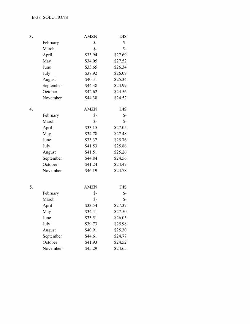
B-38 SOLUTIONS
3. AMZN DIS February $- $- March $- $- April $33.94 $27.69 May $34.05 $27.52 June $33.65 $26.34 July $37.92 $26.09 August $40.31 $25.34 September $44.38 $24.99 October $42.62 $24.56 November $44.38 $24.52
4. AMZN DIS February $- $- March $- $- April $33.15 $27.05 May $34.78 $27.48 June $33.37 $25.76 July $41.53 $25.86 August $41.51 $25.26 September $44.84 $24.56 October $41.24 $24.47 November $46.19 $24.78
5. AMZN DIS February $- $- March $- $- April $33.54 $27.37 May $34.41 $27.50 June $33.51 $26.05 July $39.73 $25.98 August $40.91 $25.30 September $44.61 $24.77 October $41.93 $24.52 November $45.29 $24.65

CHAPTER 8 B-39
6. MSI 1 0.5200 2 0.5333 3 0.4733 4 0.5467 5 0.5800
If the MSI is used as a contrarian indicator, the market appears to be headed upward, although the
indicator is relatively neutral at the moment.
7. Price Up/Down Price times
Volume Positive Money
Flow Negative Money
Flow Net Money
Flow $84.12 $84.16 + $420,800.00 $420,800.00 $84.15 - $201,960.00 $201,960.00 $84.17 + $151,506.00 $572,306.00 $84.19 + $286,246.00 $858,552.00 $84.23 + $143,191.00 $1,001,743.00 $84.20 - $387,320.00 $589,280.00 Money flow at the end of the day $412,463.00
In this case, the money flow is a bullish signal. 8. Simple Exponential 8-Nov-05 - - 9-Nov-05 - - 10-Nov-05 1,223.40 1,227.18 11-Nov-05 1,228.78 1,231.75 14-Nov-05 1,233.15 1,233.45 15-Nov-05 1,232.50 1,230.75 16-Nov-05 1,231.33 1,231.27 17-Nov-05 1,234.34 1,238.57 18-Nov-05 1,240.76 1,244.52 21-Nov-05 1,248.64 1,251.75
The reason to calculate the moving average on an index is the same for an individual stock. It can
give an indication of whether the market as a whole is moving upward or downward compared to its recent past. If the index closed above the 3-day moving average, it would be a buy indicator.
9. There appears to be a support level at $17 and a resistance level at $20. A support level is a level
below which the stock or market is unlikely to go. A resistance level is a level above which the stock or market is likely to rise.
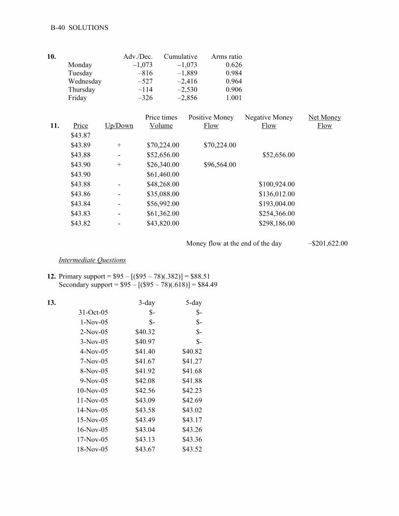
B-40 SOLUTIONS
10. Adv./Dec. Cumulative Arms ratio Monday –1,073 –1,073 0.626 Tuesday –816 –1,889 0.984 Wednesday –527 –2,416 0.964 Thursday –114 –2,530 0.906 Friday –326 –2,856 1.001
11. Price Up/Down Price times
Volume Positive Money
Flow Negative Money
Flow Net Money
Flow $43.87 $43.89 + $70,224.00 $70,224.00 $43.88 - $52,656.00 $52,656.00 $43.90 + $26,340.00 $96,564.00 $43.90 $61,460.00 $43.88 - $48,268.00 $100,924.00 $43.86 - $35,088.00 $136,012.00 $43.84 - $56,992.00 $193,004.00 $43.83 - $61,362.00 $254,366.00 $43.82 - $43,820.00 $298,186.00 Money flow at the end of the day –$201,622.00
Intermediate Questions
12. Primary support = $95 – [($95 – 78)(.382)] = $88.51 Secondary support = $95 – [($95 – 78)(.618)] = $84.49 13. 3-day 5-day 31-Oct-05 $- $- 1-Nov-05 $- $- 2-Nov-05 $40.32 $- 3-Nov-05 $40.97 $- 4-Nov-05 $41.40 $40.82 7-Nov-05 $41.67 $41.27 8-Nov-05 $41.92 $41.68 9-Nov-05 $42.08 $41.88 10-Nov-05 $42.56 $42.23 11-Nov-05 $43.09 $42.69 14-Nov-05 $43.58 $43.02 15-Nov-05 $43.49 $43.17 16-Nov-05 $43.04 $43.26 17-Nov-05 $43.13 $43.36 18-Nov-05 $43.67 $43.52

CHAPTER 8 B-41
14. 3-day 5-day 31-Oct-05 $- $- 1-Nov-05 $- $- 2-Nov-05 $40.70 $- 3-Nov-05 $41.26 $- 4-Nov-05 $41.49 $41.26 7-Nov-05 $41.77 $41.62 8-Nov-05 $42.11 $42.04 9-Nov-05 $42.08 $42.00 10-Nov-05 $42.94 $42.86 11-Nov-05 $43.49 $43.39 14-Nov-05 $43.55 $43.32 15-Nov-05 $43.27 $43.10 16-Nov-05 $42.79 $42.84 17-Nov-05 $43.47 $43.62 18-Nov-05 $44.17 $44.19
$40.50
$41.00
$41.50
$42.00
$42.50
$43.00
$43.50
$44.00
30-Oct-05 4-Nov-05 9-Nov-05 14-Nov-05 19-Nov-05
3-day5-day
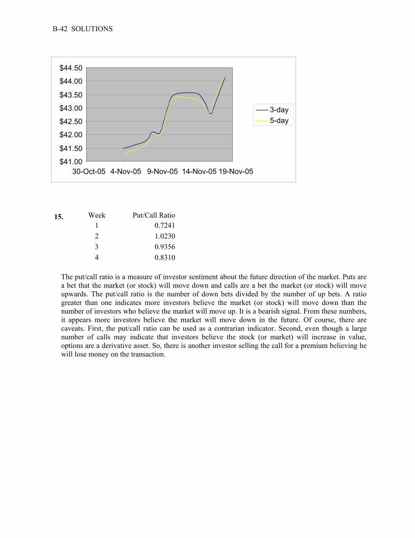
B-42 SOLUTIONS
15. Week Put/Call Ratio
1 0.7241
2 1.0230
3 0.9356
4 0.8310 The put/call ratio is a measure of investor sentiment about the future direction of the market. Puts are
a bet that the market (or stock) will move down and calls are a bet the market (or stock) will move upwards. The put/call ratio is the number of down bets divided by the number of up bets. A ratio greater than one indicates more investors believe the market (or stock) will move down than the number of investors who believe the market will move up. It is a bearish signal. From these numbers, it appears more investors believe the market will move down in the future. Of course, there are caveats. First, the put/call ratio can be used as a contrarian indicator. Second, even though a large number of calls may indicate that investors believe the stock (or market) will increase in value, options are a derivative asset. So, there is another investor selling the call for a premium believing he will lose money on the transaction.
$41.00
$41.50
$42.00
$42.50
$43.00
$43.50
$44.00
$44.50
30-Oct-05 4-Nov-05 9-Nov-05 14-Nov-05 19-Nov-05
3-day5-day
Chapter 9 Interest Rates
Concept Questions 1. Short-term rates have ranged between zero and 14 percent. Long-term rates have fluctuated between
about two and 13 percent. Long-term rates, which are less volatile, have historically been in the four-to-five percent range (the 1960 - 1980 experience is the exception). Short-term rates have about the same typical values, but more volatility (and lower rates in the unusual 1930 - 1960 period).
2. A pure discount security is a financial instrument that promises a single fixed payment (the face
value) in the future with no other payments in between. Such a security sells at a discount relative to its face value, hence the name. Treasury bills and commercial paper are two examples.
3. The Fed funds rate is set in a very active market by banks borrowing and lending from each other.
The discount rate is set by the Fed at whatever level the Fed feels is appropriate. The Fed funds rate changes all the time; the discount rate only changes when the Fed decides; the Fed funds rate is therefore much more volatile. The Fed funds market is much more active. Banks usually borrow from the Fed only as a last resort, which is the primary reason for the Fed’s discount rate-based lending.
4. Both are pure discount money market instruments. T-bills, of course, are issued by the government;
while commercial paper is issued by corporations. The primary difference is that commercial paper has default risk, so it offers a higher interest rate.
5. LIBOR is the London Interbank Offered Rate. It is the interest rate offered by major London banks
for dollar-denominated deposits. Interest rates on loans are often quoted on a LIBOR–plus basis, so the LIBOR is an important, fundamental rate in business lending, among other things.
6. Such rates are much easier to compute by hand; they predate (by hundreds of years or more)
computing machinery. 7. They are coupon interest, note principal, and bond principal, respectively. Recalling that each
STRIPS represents a particular piece of a Treasury note or bond, these designations tell us which piece is which. A “ci” is one of the many coupon payments on a note or bond; an “np” is the final principal payment on a Treasury note; and a “bp” is the final principal payment on a Treasury bond.
8. We observe nominal rates almost exclusively. Which one is more relevant actually depends on the
investor and, more particularly, what the proceeds from the investment will be used for. If the proceeds are needed to make payments that are fixed in nominal terms (like a loan repayment, perhaps), then nominal rates are more important. If the proceeds are needed to purchase real goods (like groceries) and services, then real rates are more important.
9. Trick question! It depends. Municipals have a significant tax advantage, but they also have default
risk. Low risk municipals usually have lower rates; higher risk municipals can (and often do) have higher rates.

B-44 SOLUTIONS
10. AIMR suggested answer: a. The pure expectations theory states the term structure of interest rates is explained entirely by
interest rate expectations. The theory assumes that forward rates of interest embodied in the term structure are unbiased estimates of expected future spot rates of interest. Thus, the pure expectations theory would account for a declining yield curve by arguing that interest rates are expected to fall in the future rather than rise. Investors are indifferent to holding (1) a short-term bond at a higher rate to be rolled over at a lower expected future short-term rate, and (2) a longer-term bond at a rate between the higher short-term rate and the lower expected future short-term rate.
b. Liquidity preference theory (Maturity preference) states that the term structure is a combination of
future interest rate expectations and an uncertainty “risk” or uncertainty yield “premium.” The longer the maturity of a bond, the greater the perceived risk (in terms of fluctuations of value) to the investor, who accordingly prefers to lend short term and thus requires a premium to lend longer term. This yield “premium” is added to the longer-term interest rates to compensate investors for their additional risk. Theoretically, liquidity preference could account for a downward slope if future expected rates were lower than current rates by an amount greater than their respective term risk premium. Liquidity preference theory is consistent with any shape of the term structure but suggests and upward bias or “tilt” to any term structure shape given by unbiased expectations.
c. Market segmentation theory states that the term structure results from different market participants
establishing different yield equilibriums between buyers and seller of funds at different maturity preferences. Market segmentation theory can account for any term structure shape because of the different supply/demand conditions posted at maturity ranges. Borrowers and lenders have preferred maturity ranges, based largely on institutional characteristics, and the yield curve is the average of these different suppliers’ and demanders’ maturity preferences. These maturity preferences are essentially fixed; that is, the participants do not tend to move between or among maturity ranges, so different supply and demand conditions exist across the maturity spectrum. In each maturity range, a higher demand for funds (supply of bonds) relative to the supply of funds will drive bond prices down, and rates up, in that maturity range. A downward sloping yield curve, in the context of market segmentation, indicates that a larger supply of short-term debt relative to demand has led to lower short-term bond prices and/or a small supply of long-term debt relative to demand has led to higher long-term bond prices. Either set of supply/demand conditions works to drive long-term rates lower and short-term rates higher.
Solutions to Questions and Problems NOTE: All end of chapter problems were solved using a spreadsheet. Many problems require multiple steps. Due to space and readability constraints, when these intermediate steps are included in this solutions manual, rounding may appear to have occurred. However, the final answer for each problem is found without rounding during any step in the problem. Core Question 1. Price = $100 / (1 + .056/2)2(7) = $68.8674 = $68.8674/$100 = 68.8674% or 68:28 2. Price = $100,000 / (1 + .069/2)2(7.5) = $60,123.27 = $60,123.27/$100,000 = 60.1233% or 60:04 3. YTM = 2 × [(100 / 78.75)1/(2 × 6) – 1] = .0402
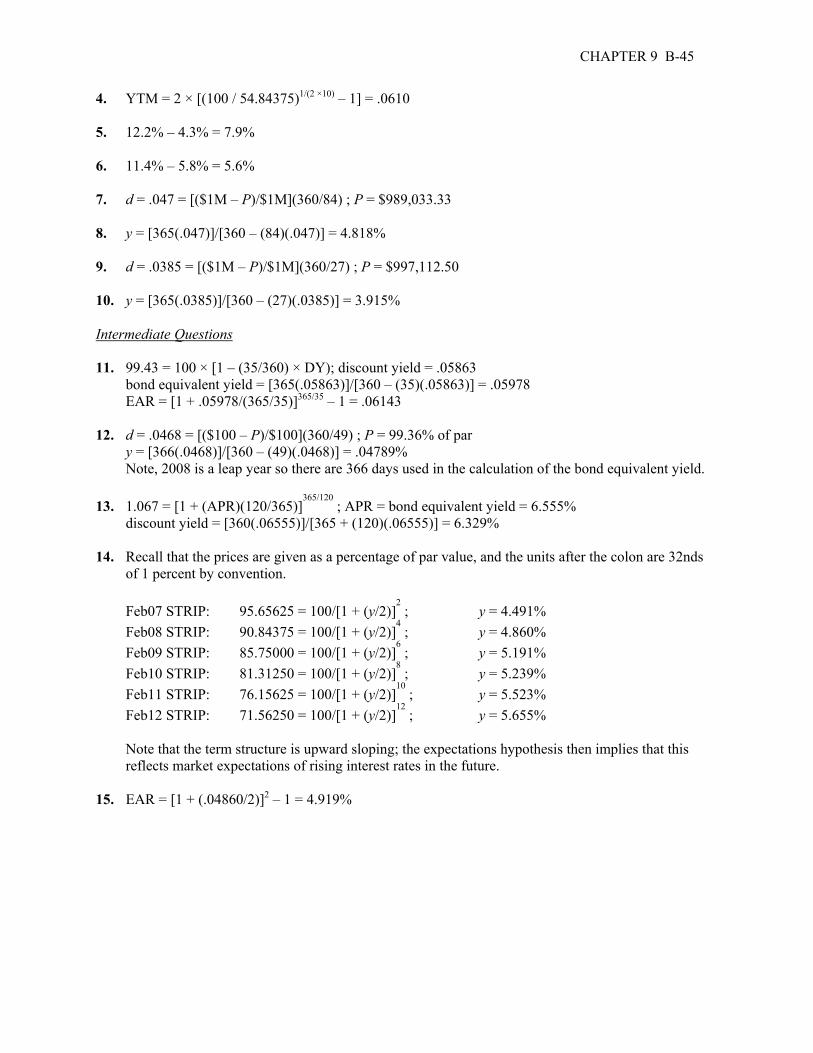
CHAPTER 9 B-45
4. YTM = 2 × [(100 / 54.84375)1/(2 ×10) – 1] = .0610 5. 12.2% – 4.3% = 7.9% 6. 11.4% – 5.8% = 5.6% 7. d = .047 = [($1M – P)/$1M](360/84) ; P = $989,033.33 8. y = [365(.047)]/[360 – (84)(.047)] = 4.818% 9. d = .0385 = [($1M – P)/$1M](360/27) ; P = $997,112.50 10. y = [365(.0385)]/[360 – (27)(.0385)] = 3.915% Intermediate Questions 11. 99.43 = 100 × [1 – (35/360) × DY); discount yield = .05863 bond equivalent yield = [365(.05863)]/[360 – (35)(.05863)] = .05978 EAR = [1 + .05978/(365/35)]365/35 – 1 = .06143 12. d = .0468 = [($100 – P)/$100](360/49) ; P = 99.36% of par y = [366(.0468)]/[360 – (49)(.0468)] = .04789% Note, 2008 is a leap year so there are 366 days used in the calculation of the bond equivalent yield. 13. 1.067 = [1 + (APR)(120/365)]
365/120 ; APR = bond equivalent yield = 6.555%
discount yield = [360(.06555)]/[365 + (120)(.06555)] = 6.329% 14. Recall that the prices are given as a percentage of par value, and the units after the colon are 32nds
of 1 percent by convention. Feb07 STRIP: 95.65625 = 100/[1 + (y/2)]
2 ; y = 4.491%
Feb08 STRIP: 90.84375 = 100/[1 + (y/2)]4 ; y = 4.860%
Feb09 STRIP: 85.75000 = 100/[1 + (y/2)]6 ; y = 5.191%
Feb10 STRIP: 81.31250 = 100/[1 + (y/2)]8 ; y = 5.239%
Feb11 STRIP: 76.15625 = 100/[1 + (y/2)]10
; y = 5.523% Feb12 STRIP: 71.56250 = 100/[1 + (y/2)]
12 ; y = 5.655%
Note that the term structure is upward sloping; the expectations hypothesis then implies that this
reflects market expectations of rising interest rates in the future. 15. EAR = [1 + (.04860/2)]2 – 1 = 4.919%

B-46 SOLUTIONS
16. [1 + (.04860/2)]4 = [1 + (.04491/2)]2 (1 + f 1,1); f1,1 = 5.298% = EAR f1,1 = 100/[1.05268] = 94.9690% of par = 94:31 rounded to the nearest 32nd. Note that this price can be found directly from the relationship ft,k = 100Pt,k/Pt; where the first
subscript refers to the time when the forward rate/price begins, the second subscript refers to the length of the forward rate/price, and P represents current or spot prices of various maturities. Similarly, ft,k = [(Pt/Pt+k)]
1/n – 1. Thus: f1,1 = 100(90.84375/95.65625) = 94.9690 ; f1,1 = (95.65625/90.84375) – 1 = 5.298% The implied 1-year forward rate is larger than the current 1-year spot rate, reflecting the expectation
that interest rates will go up in the future. Hence, for upward-sloping term structures, the implied forward rate curve lies above the spot rate curve.
17. f1,5 = 100(71.5625/95.65625) = 74.8122% of par = 74:26 rounded to the nearest 32nd. 74.8122 = 100/(1 + f1,5)
5 ; f1,5 = 5.976% f3,2 = 100(76.15625/85.75) = 88.8120% of par = 88:26 rounded to the nearest 32nd. 88.8120 = 100/(1 + f3,2)2 ; f3,2 = 6.112% 18. [1 + (.04860/2)]4 = [1 + (.04491/2)]2 (1 + f1,1 + .0030) ; f1,1 = 4.998% f1,1 = 100/(1.04998) = 95.2403% of par = 95:08 rounded to the nearest 32nd. Intuitively, the maturity premium on 2-year investments makes the future 1-year STRIP more
valuable; hence, the forward price is greater and the forward rate lower. Alternatively, verify that if the forward rate and 1-year spot rate stayed the same as before, the spot 2-year price would become 90.5168% of par and the corresponding yield would be 5.108%; i.e., the longer maturity investment would be less valuable.
19. Feb07 STRIPS: P* = 100/[1 + (.0491 + .0025) / 2 ]
2 = 95.4228% of par
∆%P = (95.4228 – 995.6563)/95.6563 = – 0.244% Feb09 STRIPS: P* = 100/[1 + (.05191 + .0025) / 2 ]
6 = 85.1258% of par
∆%P = (85.1258 – 85.7500)/85.7500 = – 0.728% Feb12 STRIPS: P* = 100/[1 + (.05655 + .0025) / 2 ]
12 = 70.5268% of par
∆%P = (70.5268 – 71.5625)/71.5625 = – 1.447% For equal changes in yield, the longer the maturity, the greater the percentage price change. Hence,
for parallel yield curve shifts, the price volatility is greater for longer-term instruments.

CHAPTER 9 B-47
Feb07 STRIPS: 95.6563 – .50 = 100/[1 + (y*/2)]2; y* = 5.027% ∆y = 5.027 – 4.491 = + 0.536% ; ∆% = .536/4.491 = 11.95% Feb09 STRIPS: 85.7500 – .50 = 100/[1 + (y*/2)]6’; y* = 5.391% ∆y = 5.391 – 5.191 = + 0.500% ; ∆% = .500/5.191 = 3.85% Feb12 STRIPS: 71.5625 – .50 = 100/[1 + (y*/2)]
12 ; y* = 5.775%
∆y = 5.775 – 5.655 = + 0.120% ; ∆% = .120/5.655 = 2.13% For equal changes in price, the absolute yield volatility is greater the shorter the maturity; the effect
is magnified for percentage yield volatility when the yield curve is upward sloping, because yields (the divisor) are smaller for short maturities. Because of this, note that for sharply downward sloping yield curves, it’s possible for shorter maturity instruments to have less percentage yield volatility, but greater absolute yield volatility, than slightly longer maturity instruments.
20. Approximate real rate = 4.24% – 3.50% = 0.74% Real interest rates are not observable because they do not correspond to any traded asset (at least not
until very recently in the U.S.); hence, they must be inferred from nominal interest rates (which do correspond to traded assets), and from estimated inflation data. Real interest rate estimates are therefore only as good as (1) the inflation estimates used in the Fisher relation and (2) the degree to which the Fisher relation itself actually describes the behavior of economic agents.
21. f1,1 = (1.0572/1.049)1/1 – 1 = 6.51% f1,2 = (1.0643/1.049)1/2 – 1 = 7.16% f1,3 = (1.0714/1.049)1/3 – 1 = 7.84% 22. f2,1 = 1.0643/1.0572 – 1 = 7.81% f3,1 = 1.0714/1.0643 – 1 = 9.23% 23. I1 = r1 – 2% = 4.90% – 2% = 2.90% I2 = f1,1 – 2% = 6.51% – 2% = 4.51% I3 = f2,1 – 2% = 7.81% – 2% = 5.81% I4 = f3,1 – 2% = 9.23% – 2% = 7.23%

B-48 SOLUTIONS
Spreadsheet Problems

Chapter 10 Bond Prices and Yields
Concept Questions 1. Premium (par, discount) bonds are bonds that sell for more than (the same as, less than) their face or
par value. 2. The face value is normally $1,000 per bond. The coupon is expressed as a percentage of face value
(the coupon rate), so the annual dollar coupon is calculated by multiplying the coupon rate by $1,000. Coupons are normally paid semi-annually; the semi-annual coupon is equal to the annual coupon divided by two.
3. The coupon rate is the annual dollar coupon expressed as a percentage of face value. The current
yield is the annual dollar coupon divided by the current price. If a bond’s price rises, the coupon rate won’t change, but the current yield will fall.
4. Interest rate risk refers to the fact that bond prices fluctuate as interest rates change. Lower coupon
and longer maturity bonds have greater interest rate risk. 5. For a premium bond, the coupon rate is higher than the yield. The reason is simply that the bonds
sell at a premium because it offers a coupon rate that is high relative to current market required yields. The reverse is true for a discount bond: it sells at a discount because its coupon rate is too low.
6. A bond’s promised yield is an indicator of what an investor can expect to earn if (1) all of the bond’s
promised payments are made and (2) market conditions do not change. The realized yield is the actual, after-the-fact return the investor receives. The realized yield is more relevant, of course, but it is not knowable ahead of time. A bond’s calculated yield to maturity is the promised yield.
7. The yield to maturity is the required rate of return on a bond expressed as a nominal annual interest
rate. For noncallable bonds, the yield to maturity and required rate of return are interchangeable terms. Unlike YTM and required return, the coupon rate is not used as the interest rate in bond cash flow valuation, but is a fixed percentage of par over the life of the bond used to set the coupon payment amount. For the example given, the coupon rate on the bond is still 10 percent, and the YTM is 8 percent.
8. The yield to maturity is the required rate of return on a bond expressed as a nominal annual interest
rate. For noncallable bonds, the yield to maturity and required rate of return are interchangeable terms. Unlike YTM and required return, the coupon rate is not used as the interest rate in bond cash flow valuation, but is a fixed percentage of par over the life of the bond used to set the coupon payment amount. For the example given, the coupon rate on the bond is still 10 percent, and the YTM is 8 percent.
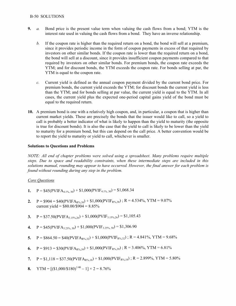
B-50 SOLUTIONS
9. a. Bond price is the present value term when valuing the cash flows from a bond; YTM is the interest rate used in valuing the cash flows from a bond. They have an inverse relationship.
b. If the coupon rate is higher than the required return on a bond, the bond will sell at a premium,
since it provides periodic income in the form of coupon payments in excess of that required by investors on other similar bonds. If the coupon rate is lower than the required return on a bond, the bond will sell at a discount, since it provides insufficient coupon payments compared to that required by investors on other similar bonds. For premium bonds, the coupon rate exceeds the YTM; and for discount bonds, the YTM exceeds the coupon rate. For bonds selling at par, the YTM is equal to the coupon rate.
c. Current yield is defined as the annual coupon payment divided by the current bond price. For
premium bonds, the current yield exceeds the YTM; for discount bonds the current yield is less than the YTM; and for bonds selling at par value, the current yield is equal to the YTM. In all cases, the current yield plus the expected one-period capital gains yield of the bond must be equal to the required return.
10. A premium bond is one with a relatively high coupon, and, in particular, a coupon that is higher than
current market yields. These are precisely the bonds that the issuer would like to call, so a yield to call is probably a better indicator of what is likely to happen than the yield to maturity (the opposite is true for discount bonds). It is also the case that the yield to call is likely to be lower than the yield to maturity for a premium bond, but this can depend on the call price. A better convention would be to report the yield to maturity or yield to call, whichever is smaller.
Solutions to Questions and Problems NOTE: All end of chapter problems were solved using a spreadsheet. Many problems require multiple steps. Due to space and readability constraints, when these intermediate steps are included in this solutions manual, rounding may appear to have occurred. However, the final answer for each problem is found without rounding during any step in the problem. Core Questions 1. P = $45(PVIFA4.1%, 30) + $1,000(PVIF4.1%, 30) = $1,068.34 2. P = $904 = $40(PVIFAR%,38) + $1,000(PVIFR%,38) ; R = 4.534%, YTM = 9.07% current yield = $80.00/$904 = 8.85% 3. P = $37.50(PVIFA3.15%,26) + $1,000(PVIF3.15%,26) = $1,105.43 4. P = $45(PVIFA3.25%, 50) + $1,000(PVIF3.25%, 50) = $1,306.90 5. P = $864.50 = $40(PVIFAR%,32) + $1,000(PVIFR%,32) ; R = 4.841%, YTM = 9.68% 6. P = $913 = $30(PVIFAR%,39) + $1,000(PVIFR%,39) ; R = 3.406%, YTM = 6.81% 7. P = $1,118 = $37.50(PVIFAR%,18) + $1,000(PVIFR%,18) ; R = 2.899%, YTM = 5.80% 8. YTM = [($1,000/$180)1/40 – 1] × 2 = 8.76%

CHAPTER 10 B-51
9. YTC = [($500/$180)1/20 – 1] × 2 = 10.48% 10. YTC = [($475/$180)1/10 – 1] × 2 = 9.94% Intermediate Questions 11. P = $1,082.20 = $C(PVIFA3.75%,26) + $1,000(PVIFA3.75%,26) ; C = $42.50 coupon rate = 2(0.0425) = 8.50% 12. P = $47(PVIFA4.51%,38) + $1,000(PVIF4.51%,38) = $1,034.25 13. P = $780 = $42.50(PVIFAR%,56) + $1,000(PVIFR%,56) ; R = 5.529%; YTM = 11.06%
14. Assuming a $1,000 face value, the current price of the bond is $1,000 / (1.04)40 = $208.29. Two
years later the bond has 13 years to maturity and the same price, so the new yield to maturity must be [($1,000/$208.29)1/36 – 1] × 2 = 8.91%.
15. If held to maturity, a zero-coupon bond will always have a realized yield equal to its original yield to
maturity, which in this case is 8 percent. 16. P: P0 = $45(PVIFA3.5.5%,30) + $1,000(PVIF3.5.5%,30) = $1,183.92 P1 = $45(PVIFA3.5.5%,28) + $1,000(PVIF3.5.5%,28) = $1,176.67 P5 = $45(PVIFA3.5.5%,20) + $1,000(PVIF3.5.5%,20) = $1,142.12 P10 = $45(PVIFA3.5.5%,10) + $1,000(PVIF3.5.5%,10) = $1,083.17 P14 = $45(PVIFA3.5.5%,2) + $1,000(PVIF3.5.5%,2) = $1,019.00
P15 = $1,000 D: P0 = $45(PVIFA5.5%,30) + $1,000(PVIF5.5%,30) = $854.66 P1 = $45(PVIFA5.5%,28) + $1,000(PVIF5.5%,28) = $858.79 P5 = $45(PVIFA5.5%,20) + $1,000(PVIF5.5%,20) = $880.50 P10 = $45(PVIFA5.5%,10) + $1,000(PVIF5.5%,10) = $924.62 P14 = $45(PVIFA5.5%,2) + $1,000(PVIF5.5%,2) = $981.54
P15 = $1,000
All else held equal, the premium over par value for a premium bond declines as maturity is approached, and the discount from par value for a discount bond declines as maturity is approached. This is sometimes called the “pull to par.”
17. If both bonds sell at par, the initial YTM on both bonds is the coupon rate, 8 percent. If the YTM
suddenly rises to 10 percent, then: PA = $40(PVIFA5%,4) + $1,000(PVIF5%,4) = $964.54 PB = $40(PVIFA5%,30) + $1,000(PVIF5%,30) = $846.28 ∆PA% = (964.54 – 1,000)/1,000 = – 3.55% ∆PB% = (846.28 – 1,000)/1,000 = – 15.37%

B-52 SOLUTIONS
If the YTM suddenly falls to 6 percent, then: PA = $40(PVIFA3%,4) + $1,000(PVIF3%,4) = $1,037.17 PB = $40(PVIFA3%,30) + $1,000(PVIF3%,30) = $1,196.00 ∆PA% = (1,037.17 – 1,000)/1,000 = + 3.72% ∆PB% = (1,196.00 – 1,000)/1,000 = + 29.60%
All else the same, the longer the maturity of a bond, the greater is its price sensitivity to changes in interest rates.
18. Initially, at a YTM of 7 percent, the prices of the two bonds are: PJ = $25(PVIFA3.5%,20) + $1,000(PVIF3.5%,20) = $857.88 PK = $45(PVIFA3.5%,20) + $1,000(PVIF3.5%,20) = $1,142.12 If the YTM rises from 7 percent to 9 percent: PJ = $25(PVIFA4.5%,20) + $1,000(PVIF4.5%,20) = $739.84 PK = $45(PVIFA4.5%,20) + $1,000(PVIF4.5%,20) = $1,000.00 ∆PJ = (739.84 – 857.88)/857.88 = – 13.76% ∆PK = (1,000.00 – 1,142.12)/1,142.12 = – 12.44% If the YTM declines from 7 percent to 5 percent: PJ = $25(PVIFA2.5%,20) + $1,000(PVIF2.5%,20) = $1,000.00 PK = $45(PVIFA2.5%,20) + $1,000(PVIF2.5%,20) = $1,311.78 ∆PJ = (1,000.00 – 857.88)/857.88 = + 16.57% ∆PK = (1,311.78 – 1,142.12)/1,142.12 = + 14.85%
All else the same, the lower the coupon rate on a bond, the greater is its price sensitivity to changes in interest rates.
19. Current yield = .0722 = $75/P0 ; P0 = $75/.0722 = $1,038.78 P0 = $1,038.78 = $37.50[ (1 – (1/1.0349)
N ) / .0349 ] + $1,000/1.0349N
1,038.78(1.0349)
N = 1074.50(1.0349)N – 1,074.50 + 1,000
74.50 = 35.72(1.0349)N ; 2.0857 = 1.0349N ; N = log 2.0857 / log 1.0349 = 21.43 = 10.71 yrs.
20. The maturity is indeterminate; a bond selling at par can have any maturity length. 21. a. P0 = $1,080 = $45(PVIFAR%,30) + $1,000(PVIFR%,30) ; R = 4.035%, YTM = 8.07%
This is the rate of return you expect to earn on your investment when you purchase the bond.

CHAPTER 10 B-53
b. Price when sold = $45(PVIFA3.035%,26) + $1,000(PVIF3.035%,26) = $923.32 Future value of reinvested interest payments = $45(FVIFA4.035%,4) = $191.19 Realized return = ($923.32 – 1,080 + 191.19) / $1,080 = 3.20% The realized yield is less than the expected yield when the bond was purchased because interest
rates have increased by 2 percent; bond prices fall when yields rise. 22. The yield to call can be computed as: P = $1,180 = $60(PVIFAR%,30) + $1,080(PVIFR%,30) ; R = 4.674%, YTC = 9.35%
Since the bond sells at a premium to par value, you know the coupon rate must be greater than the yield. Thus, if interest rates remain at current levels, the bond issuer will likely call the bonds to refinance (at a lower coupon rate) at the earliest possible time, which is the date when call protection ends. The yield computed to this date is the YTC, and it will always be less than the YTM for premium bonds with a zero call premium. In the present example,
P = $1,180 = $60(PVIFAR%,40) + $1,000(PVIFR%,40) ; R = 4.957%, YTM = 9.91%
where if the bond is held until maturity, no call premium must be paid. Note that using the same analysis, a break-even call premium can also be computed:
P = $1,180 = $60(PVIFA4.957%,30) + ($1,000 + X)(PVIF4.957%,30) ; X = $161.10
Thus, if interest rates remain unchanged, the bond will not be called if the call premium is greater than $161.10.
23. P = $1,130.60 = $35(PVIFAR%,18) + $1,000(PVIFR%,18) ; R = 2.584%, YTM = 5.167%
Duration = (1.02584/.05167) – [(1.0284 + 9(.035 – .05167)) / (.05167 + .07(1.0258418 – 1))] Duration = 6.974 years
Modified duration = 6.974/(1.02584) = 6.799 years 24. Estimated percent change in price = –6.799(.02) = –.1360 = (P1/P0) – 1 so P1 = (1 – .1360)($1,130.60) = $976.87 Actual P1 = $35(PVIFA2.584%,18) + $1,000(PVIF2.584%,18) = $988.74 25. Dollar value of an 01 = (6.799/100) × $1,130.60 × .01 = $0.769
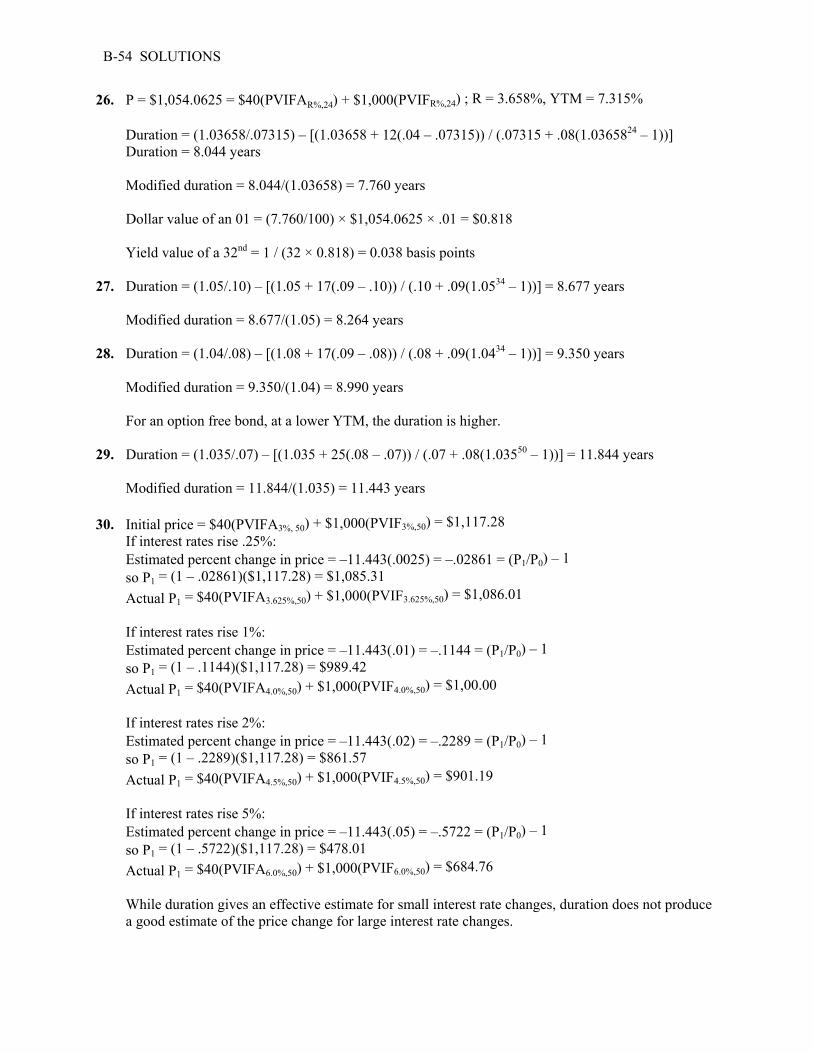
B-54 SOLUTIONS
26. P = $1,054.0625 = $40(PVIFAR%,24) + $1,000(PVIFR%,24) ; R = 3.658%, YTM = 7.315%
Duration = (1.03658/.07315) – [(1.03658 + 12(.04 – .07315)) / (.07315 + .08(1.0365824 – 1))] Duration = 8.044 years
Modified duration = 8.044/(1.03658) = 7.760 years Dollar value of an 01 = (7.760/100) × $1,054.0625 × .01 = $0.818 Yield value of a 32nd = 1 / (32 × 0.818) = 0.038 basis points 27. Duration = (1.05/.10) – [(1.05 + 17(.09 – .10)) / (.10 + .09(1.0534 – 1))] = 8.677 years Modified duration = 8.677/(1.05) = 8.264 years 28. Duration = (1.04/.08) – [(1.08 + 17(.09 – .08)) / (.08 + .09(1.0434 – 1))] = 9.350 years Modified duration = 9.350/(1.04) = 8.990 years For an option free bond, at a lower YTM, the duration is higher. 29. Duration = (1.035/.07) – [(1.035 + 25(.08 – .07)) / (.07 + .08(1.03550 – 1))] = 11.844 years Modified duration = 11.844/(1.035) = 11.443 years 30. Initial price = $40(PVIFA3%, 50) + $1,000(PVIF3%,50) = $1,117.28 If interest rates rise .25%: Estimated percent change in price = –11.443(.0025) = –.02861 = (P1/P0) – 1 so P1 = (1 – .02861)($1,117.28) = $1,085.31 Actual P1 = $40(PVIFA3.625%,50) + $1,000(PVIF3.625%,50) = $1,086.01 If interest rates rise 1%: Estimated percent change in price = –11.443(.01) = –.1144 = (P1/P0) – 1 so P1 = (1 – .1144)($1,117.28) = $989.42 Actual P1 = $40(PVIFA4.0%,50) + $1,000(PVIF4.0%,50) = $1,00.00 If interest rates rise 2%: Estimated percent change in price = –11.443(.02) = –.2289 = (P1/P0) – 1 so P1 = (1 – .2289)($1,117.28) = $861.57 Actual P1 = $40(PVIFA4.5%,50) + $1,000(PVIF4.5%,50) = $901.19 If interest rates rise 5%: Estimated percent change in price = –11.443(.05) = –.5722 = (P1/P0) – 1 so P1 = (1 – .5722)($1,117.28) = $478.01 Actual P1 = $40(PVIFA6.0%,50) + $1,000(PVIF6.0%,50) = $684.76
While duration gives an effective estimate for small interest rate changes, duration does not produce a good estimate of the price change for large interest rate changes.

CHAPTER 10 B-55
31. Strategy I: %∆ MV5 Year = –4.83(–.0075) = .036225; New MV = (1 + .036225)($5,000,000) = $5,181,125 %∆ MV25 Year = –23.81(.0050) = –.11905; New MV = (1 – .11905)($5,000,000) = $4,404,750 New market value of portfolio = $5,181,125 + 4,404,750 = $9,585,875 Strategy II: %∆ MV15 Year = –14.35(.0025) = –.035875; New MV = (1 – .035875)($10,000,000) = $9,641,250 For this interest rate change, Strategy II is a better alternative. 32. Zero coupon YTM = $952 = $1,000 / (1 + r); r = 5.04% Two year spot rate: $1,032 = $70/(1 + .0504) + $1,070/(1 + r2)2 ; r2 = 5.28% Three year spot rate: $1,060 = $80/(1 + .0504) + $80/(1 + .0528)2 + $1,080/(1 + r2)3; r3 = 5.81% 33. P = $80/(1 + .0520) + $80/(1 + .0585)2 + $80/(1 + .0615)3 + $1,080/(1 + .0675)4 = $1,046.00 P = $1,046.00 = $80(PVIFAR%,4) + $1,000(PVIFR%,4) ; YTM = 6.65% Spreadsheet Problems
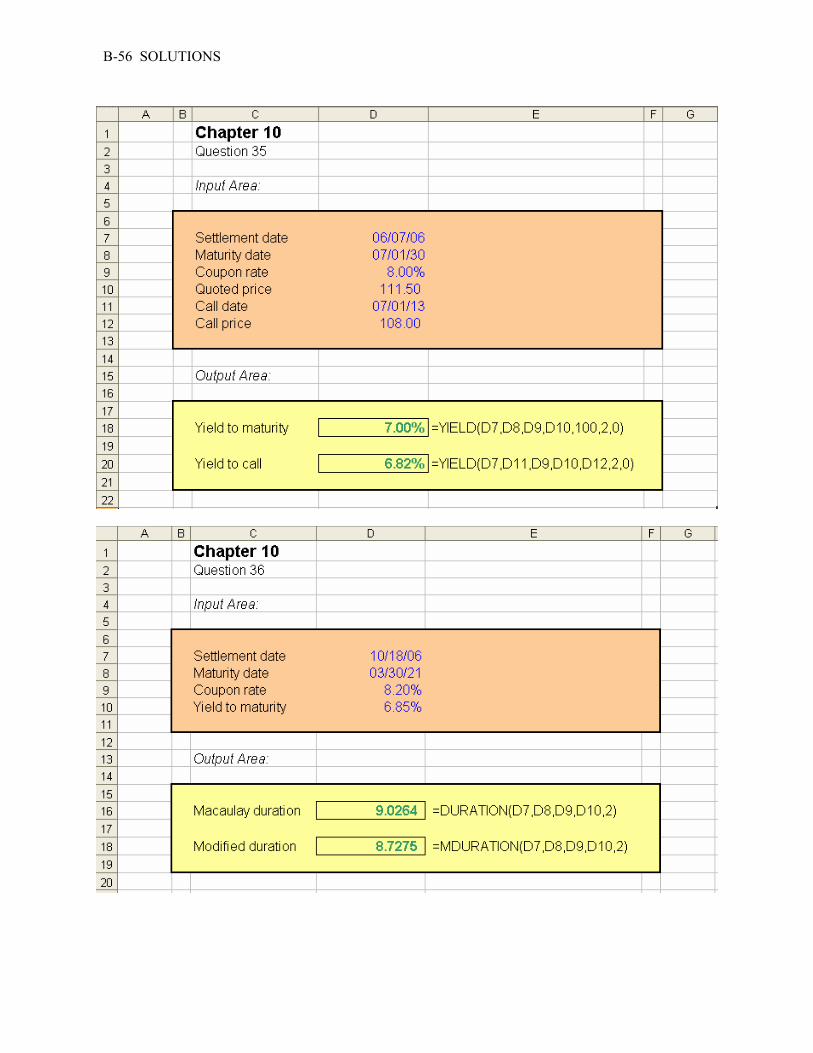
B-56 SOLUTIONS
Chapter 11 Diversification and Risky Asset Allocation
Concept Questions 1. Based on market history, the average annual standard deviation of return for a single, randomly
chosen stock is about 50 percent. The average annual standard deviation for an equally-weighted portfolio of many stocks is about 20 percent.
2. If the returns on two stocks are highly correlated, they have a strong tendency to move up and down
together. If they have no correlation, there is no particular connection between the two. If they are negatively correlated, they tend to move in opposite directions.
3. An efficient portfolio is one that has the highest return for its level of risk. 4. True. Remember, portfolio return is a weighted average of individual returns. 5. False. Remember the principle of diversification. 6. Because of the effects of diversification, an investor will never receive the highest return possible
from a single asset. However, the investor will also never receive the lowest return. More importantly, even though an investor does give up the potential “home run” investment, the reduction in return is more than offset by the reduction in risk. In other words, you give up a little return for a lot less risk.
7. You know your current portfolio is the minimum variance portfolio (or below). Below and to the
right of the minimum variance portfolio, as you add more of the lower risk asset, the standard deviation of your portfolio increases and the expected return decreases.
8. The importance of the minimum variance portfolio is that it determines the lower bond of the
efficient frontier. While there are portfolios on the investment opportunity set to the right and below the minimum variance portfolio, they are inefficient. That is, there is a portfolio with the same level of risk and a higher return. No rational investor would ever invest in a portfolio below the minimum variance portfolio.
9. False. Individual assets can lie on the efficient frontier depending on its expected return, standard
deviation, and correlation with all other assets. 10. If two assets have zero correlation and the same standard deviation, then evaluating the general
expression for the minimum variance portfolio shows that x = ½; in other words, an equally-weighted portfolio is minimum variance.

B-58 SOLUTIONS
Solutions to Questions and Problems NOTE: All end of chapter problems were solved using a spreadsheet. Many problems require multiple steps. Due to space and readability constraints, when these intermediate steps are included in this solutions manual, rounding may appear to have occurred. However, the final answer for each problem is found without rounding during any step in the problem. Core Questions 1. .2(–.10) + .6(.14) + .2(.27) = 11.80% 2. .2(–.10 – .1180)2 + .4(.14 – .1180)2 + .2(.27 – .1180)2 = .01442; σ = 12.01% 3. (1/3)(–.10) + (1/3)(.14) + (1/3)(.27) = 10.33% (1/3)(–.10 – .1033)2 + (1/3)(.14 – .1033)2 + (1/3)(.27 – .1033)2 = .02349; σ = 15.33% 4.
Calculating Expected Returns
Roll Ross
(1) State of
Economy
(2) Probability of State
of Economy
(3) Return if
State Occurs
(4) Product (2) × (3)
(5) Return if
State Occurs
(6) Product (2) × (5)
Bust .40 –10% –.0400 21% .0840Boom .60 28% .1680 8% .0480 E(R) = 12.80% E(R) = 13.20%
5.
(1) State
of Economy
(2) Probability of
State of Economy
(3) Return Deviation
from Expected Return
(4) Squared Return
Deviation
(5) Product (2) × (4)
Roll Bust .40 –.2280 .0520 .0208 Boom .60 .1520 .0231 .0139 σ2 = .0347 Ross Bust .40 .0780 .0061 .0024 Boom .60 –.0520 .0027 .0016 σ2 = .0041
Taking square roots, the standard deviations are 18.62% and 6.37%.
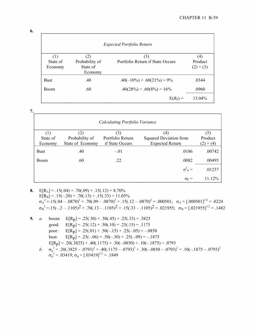
CHAPTER 11 B-59
6.
Expected Portfolio Return
(1) State of
Economy
(2) Probability of
State of Economy
(3) Portfolio Return if State Occurs
(4) Product (2) × (3)
Bust
.40
.40(–10%) + .60(21%) = 9%
.0344
Boom
.60
.40(28%) + .60(8%) = 16%
.0960
E(RP) =
13.04%
7.
Calculating Portfolio Variance
(1)
State of Economy
(2) Probability of
State of Economy
(3) Portfolio Return if State Occurs
(4) Squared Deviation from
Expected Return
(5) Product (2) × (4)
Bust
.40
–.01
.0186
.00742
Boom
.60
.22
.0082
.00495
σ2
P =
.01237
σP =
11.12%
8. E[RA] = .15(.04) + .70(.09) + .15(.12) = 8.70% E[RB] = .15(–.20) + .70(.13) + .15(.33) = 11.05% σA
2 =.15(.04 – .0870)2 + .70(.09 – .0870)2 + .15(.12 – .0870)2 = .000501; σA = [.000501]1/2 = .0224 σB
2 =.15(–.2 – .1105)2 + .70(.13 – .1105)2 + .15(.33 – .1105)2 = .021955; σB = [.021955]1/2 = .1482 9. a. boom: E[Rp] = .25(.30) + .50(.45) + .25(.33) = .3825 good: E[Rp] = .25(.12) + .50(.10) + .25(.15) = .1175 poor: E[Rp] = .25(.01) + .50(–.15) + .25(–.05) = –.0850 bust: E[Rp] = .25(–.06) + .50(–.30) + .25(–.09) = –.1875 E[Rp] = .20(.3825) + .40(.1175) + .30(–.0850) + .10(–.1875) = .0793 b. σp
2 = .20(.3825 – .0793)2 + .40(.1175 – .0793)2 + .30(–.0850 – .0793)2 + .10(–.1875 – .0793)2 σp
2 = .03419; σp = [.03419]1/2 = .1849

B-60 SOLUTIONS
10. Notice that we have historical information here, so we calculate the sample average and sample standard deviation (using n – 1) just like we did in Chapter 1. Notice also that the portfolio has less risk than either asset.
Annual Returns on Stocks A and B
Year
Stock A
Stock B Portfolio AB2001
18%
50%
40.40%
2002
40
–30
–9.00 2003
–15
45
27.00
2004
20
2
7.40 2005
4
20
15.20
Avg return 13.40 17.40 16.20
Std deviation 20.42 32.85 18.81 Intermediate Questions 11. Boom: .20(15%) + .35(18%) + .45(20%) = 18.30% Bust: .20(10%) + .35(0%) + .45(–10%) = –2.50% E(RP) = .70(.1830) + .30(–.0250) = 12.06% 2
Pσ = .70(.1830 – .1206)2 + .30(–.0250 – .1206)2 = .00909; σP = 9.53% 12. E(RP) = .40(.15) + .60(.10) = 12.00% 2
Pσ = .402(.502)+ .602(.382) + 2(.40)(.60)(.50)(.38)(.15) = .10566; σP = 32.51% 13. 2
Pσ = .402(.502) + .602(.382) + 2(.40)(.60)(.50)(.38)(1.0) = .18318; σP = 42.80% 2
Pσ = .402(.502) + .602(.382) + 2(.40)(.60)(.50)(.38)(0.0) = .09198; σP = 30.33% 2
Pσ = .402(.502) + .602(.382) + 2(.40)(.60)(.50)(.38)(–1.0) = .00078; σP = 2.80% As the correlation becomes smaller, the standard deviation of the portfolio decreases. In the extreme
with a correlation of –1, this means that as one asset has a higher than expected return, the other asset has a lower than expected return. The extra returns, whether positive or negative, will offset each other resulting in smoother portfolio return with less variance.
14. w3 Doors = .20 .38 .50 2 - .38 50
.20 .38 .60 - .3822
2
×××+××
.= 0.3435; wDoors = (1 – .3435) = .6565
E(RP) = .3435(.15) + .6565(.10) = 11.72% 2
Pσ = .34352(.502) + .65652(.382) + 2(.3435)(.6565)(.50)(.38)(.20) = .10459 σP = 32.34%
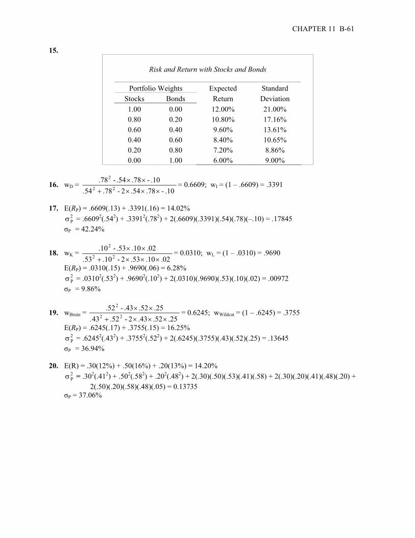
CHAPTER 11 B-61
15.
Risk and Return with Stocks and Bonds
Portfolio Weights
Expected
Standard
Stocks
Bonds
Return
Deviation
1.00
0.00 12.00% 21.00%
0.80
0.20 10.80% 17.16%
0.60
0.40 9.60% 13.61%
0.40
0.60 8.40% 10.65%
0.20
0.80 7.20% 8.86%
0.00
1.00 6.00% 9.00%
16. wD = .10- .78 .54 2 - .78 54
.10- .78 .54 - .7822
2
×××+××
.= 0.6609; wI = (1 – .6609) = .3391
17. E(RP) = .6609(.13) + .3391(.16) = 14.02% 2
Pσ = .66092(.542) + .33912(.782) + 2(.6609)(.3391)(.54)(.78)(–.10) = .17845 σP = 42.24%
18. wK = .02 .10 .53 2 - .10 53
.02 .10 .53 - .1022
2
×××+××
.= 0.0310; wL = (1 – .0310) = .9690
E(RP) = .0310(.15) + .9690(.06) = 6.28% 2
Pσ = .03102(.532) + .96902(.102) + 2(.0310)(.9690)(.53)(.10)(.02) = .00972 σP = 9.86%
19. wBruin = .25 .52 .43 2 - .52 43
.25 .52 .43 - .5222
2
×××+××
.= 0.6245; wWildcat = (1 – .6245) = .3755
E(RP) = .6245(.17) + .3755(.15) = 16.25% 2
Pσ = .62452(.432) + .37552(.522) + 2(.6245)(.3755)(.43)(.52)(.25) = .13645 σP = 36.94% 20. E(R) = .30(12%) + .50(16%) + .20(13%) = 14.20% 2
Pσ = .302(.412) + .502(.582) + .202(.482) + 2(.30)(.50)(.53)(.41)(.58) + 2(.30)(.20)(.41)(.48)(.20) + 2(.50)(.20)(.58)(.48)(.05) = 0.13735 σP = 37.06%

B-62 SOLUTIONS
21. wJ = .60 .24 .58 2 - .24 58
.60 .24 .58 - .2422
2
×××+××
.= –0.1142; wS = (1 – (–.1142)) = 1.1142
2Pσ = (–.11422)(.582) + (1.11422)(.242) + 2(.58)(.24)(–.1142)(1.1142)(.60) = .05464
σP = (.05464)1/2 = 23.38% E(RP) = –.1142(.15) + 1.1142(.06) = 8.31% Even thought it is possible to mathematically calculate the standard deviation and expected return of
a portfolio with a negative weight, an explicit assumption is that no asset can have a negative weight. The reason this portfolio has a negative weight in one asset is the relatively high correlation between the two assets. If you look at the investment opportunity sets in the chapter, you will notice that as the correlation decreases, the investment opportunity set bends further backwards. However, for a portfolio with a correlation of +1, there is no minimum variance portfolio with a variance lower than the lowest variance asset. This implies there is some necessary level of correlation to make the minimum variance portfolio have a variance lower than the lowest variance asset. The formula to determine if there is a minimum variance portfolio with a variance less than the lowest variance asset
is: max
min
σσ
> ρ. In this case, .58.24 = .414 < .60 so there is no minimum variance portfolio with a
variance lower than the lowest variance asset assuming non-negative asset weights. 22. Look at 2
Pσ : 2
Pσ = (xA × σA + xB × σB)2 = 1 x x 2 x x BABA
2B
2B
2A
2A ×σ×σ×××+σ×+σ× , which is precisely the expression for the
variance on a two–asset portfolio when the correlation is +1. 23. Look at 2
Pσ : 2
Pσ = (xA × σA – xB × σB)2 = (-1) x x 2 x x BABA
2B
2B
2A
2A ×σ×σ×××+σ×+σ× , which is precisely the expression for the
variance on a two–asset portfolio when the correlation is –1. 24. From the previous question, with a correlation of –1: σp = xA × σA – xB × σB = x × σA – (1 – x) × σB Set this to equal zero and solve for x to get: 0 = x × σA – (1 – x) × σB x = σB/ (σA + σB) This is the weight on the first asset.

CHAPTER 11 B-63
25. Let ρ stand for the correlation, then: 2
Pσ = ρ×σ×σ×××+σ×+σ× x x 2 x x BABA2B
2B
2A
2A
= x2 × σA2 + (1 – x)2 × σB
2 + 2 × x × (1 – x) × σA × σB × ρ Take the derivative with respect to x and set equal to zero: dσp
2/dx = 2 × x × σA2 – 2 × (1 – x) × σB
2 + 2 × σA × σB × ρ – 4 × x × σA × σB × ρ = 0 Solve for x to get the expression in the text.
Chapter 12 Return, Risk, and the Security Market Line
Concept Questions 1. Some of the risk in holding any asset is unique to the asset in question. By investing in a variety of
assets, this unique portion of the total risk can be almost completely eliminated at little cost. On the other hand, there are some risks that affect all investments. This portion of the total risk of an asset cannot be costlessly eliminated. In other words, systematic risk can be controlled, but only by a costly reduction in expected returns.
2. If the market expected the growth rate in the coming year to be 2 percent, then there would be no
change in security prices if this expectation had been fully anticipated and priced. However, if the market had been expecting a growth rate different than 2 percent and the expectation was incorporated into security prices, then the government's announcement would most likely cause security prices in general to change; prices would drop if the anticipated growth rate had been more than 2 percent, and prices would rise if the anticipated growth rate had been less than 2 percent.
3. a. systematic
b. unsystematic c. both; probably mostly systematic d. unsystematic e. unsystematic
f. systematic 4. a. An unexpected, systematic event occurred; market prices in general will most likely
decline. b. No unexpected event occurred; company price will most likely stay constant. c. No unexpected, systematic event occurred; market prices in general will most likely stay
constant. d. An unexpected, unsystematic event occurred; company price will most likely decline. e. No unexpected, systematic event occurred unless the outcome was a surprise; market
prices in general will most likely stay constant. 5. False. Expected returns depend on systematic risk, not total risk. 6. Earnings contain information about recent sales and costs. This information is useful for projecting
future growth rates and cash flows. Thus, unexpectedly low earnings lead market participants to reduce estimates of future growth rates and cash flows; price drops are the result. The reverse is often true for unexpectedly high earnings.
7. Yes. It is possible, in theory, for a risky asset to have a beta of zero. Such an asset’s return is simply
uncorrelated with the overall market. Based on the CAPM, this asset’s expected return would be equal to the risk-free rate. It is also possible to have a negative beta; the return would be less than the risk-free rate. A negative beta asset would carry a negative risk premium because of its value as a diversification instrument. A negative beta asset can be created by shorting an asset with a positive beta. A portfolio with a zero beta can always be created by combining long and short positions.
CHAPTER 12 B-65
8. The rule is always “buy low, sell high.” In this case, we buy the undervalued asset and sell (short) the overvalued one. It does not matter whether the two securities are misvalued with regard to some third security; all that matters is their relative value. In other words, the trade will be profitable as long as the relative misvaluation disappears; however, there is no guarantee that the relative misvaluation will disappear, so the profits are not certain.
9. If every asset has the same reward-to-risk ratio, the implication is that every asset provides the same
risk premium for each unit of risk. In other words, the only way to increase your return (reward) is to accept more risk. Investors will only take more risk if the reward is higher, and a constant reward-to-risk ratio ensures this will happen. We would expect every asset in a liquid, well-functioning to have the same reward-to-risk ratio due to competition and investor risk aversion. If an asset has a reward-to-risk ratio that is lower than all other assets, investors will avoid that asset, thereby driving the price down, increasing the expected return and the reward-to-risk ratio. Similarly, if an asset has a reward-to-risk ratio that is higher than other assets, investors will flock to the asset, increasing the price, and decreasing the expected return and the reward-to-risk ratio.
10. AIMR suggested answer: a. Systematic risk refers to fluctuations in asset prices caused by macroeconomic factors that are
common to all risky assets; hence systematic risk is often referred to as market risk. Examples of systematic risk include the business cycle, inflation, monetary policy, and technological changes. Firm-specific risk refers to fluctuations in asset prices caused by factors that are independent of the market such as industry characteristics or firm characteristics. Examples of firm-specific risk include litigation, patents, management, and financial leverage.
b. Trudy should explain to the client that picking only the top five best ideas would most likely result
in the client holding a much more risky portfolio. The total risk of the portfolio, or portfolio variance, is the combination of systematic risk and firm-specific risk. i.) The systematic component depends on the sensitivity of the individual assets to market movements as measured by beta. Assuming the portfolio is well-diversified, the number of assets will not affect the systematic risk component of portfolio variance. The portfolio beta depends on the individual security betas and the portfolio weights of those securities. ii.) On the other hand, the components of the firm-specific risk (sometimes called nonsystematic risk) are not perfectly positively correlated with each other and as more asset are added to the portfolio those additional assets tend to reduce portfolio risk. Hence, increasing the number of securities in a portfolio reduces firm-specific risk. For example, a patent expiring for one company would not affect the other securities in the portfolio. An increase in oil prices might hurt airline stock but aid an energy stock. As the number of randomly selected securities increases, the total risk (variance) of the portfolio approaches its systematic variance.
Solutions to Questions and Problems NOTE: All end of chapter problems were solved using a spreadsheet. Many problems require multiple steps. Due to space and readability constraints, when these intermediate steps are included in this solutions manual, rounding may appear to have occurred. However, the final answer for each problem is found without rounding during any step in the problem. Core Questions 1. E(Ri) = .136 = .04 + .075βi ; βi = 1.28 2. E(Ri) = .12 = .05 + (E(Rmkt) – .05)(.85); E(Rmkt) = .1324
B-66 SOLUTIONS
3. E(Ri) = .11 = Rf + (.13 – Rf)(.70); Rf = .0633 4. E(Ri) = .16 = .055 + 1.3(MRP); MRP = .0808 5. βP = .15(1.2) + .20(.6) + .25(1.5) + .40(.9) = 1.035 6. Portfolio value = 200($60) + 300($85) + 100($25) = $40,000.00 xA = 200($60)/$40,000 = .3000 xB = 300($85)/$40,000 = .6375 xC = 100($25)/$40,000 = .0625 βP = .3000(1.2) + .6375(.9) + .0625(1.6) = 1.03 7. βP = 1.0 = 1/3(0) + 1/3(1.2) + 1/3(βX) ; βX = 1.80 8. E(Ri) = .058 + (.12 – .058)(1.15) = .1293 9. E(Ri) = .045 + (.11 – .045)(1.2) = .1230 Dividend yield = $1.20/$48 = .0229 Capital gains yield = .1230 – .0229 = .1001 Price next year = $48(1 + .1001) = $52.80 10. a. E(RP) = (.15 + .06)/2 = .1050 b. βP = 0.5 = xS(1.1) + (1 – xS)(0) ; xS = 0.5/1.1 = .4545 ; xrf = 1 – .4545 = .5455 c. E(RP) = .12 = .15xS + .06(1 – xS); xS = .6667; βp = .6667(1.1) + .3333(0) = 0.73 d. βP = 1.8 = xS(1.1) + (1 – xS)(0) ; xS = 1.8/1.1 = 1.64; xrf = 1 – 1.64 = –0.64 The portfolio is invested 164% in the stock and –64% in the risk-free asset. This represents
borrowing at the risk-free rate to buy more of the stock. Intermediate Questions 11. βP = xW(1.2) + (1 – xW)(0) = 1.2xW E(RW) = .15 = .07 + MRP(1.20) ; MRP = .08/1.2 = .0667 E(RP) = .07 + .0667 βP; slope of line = MRP = .0667; E(RP) = .07 + .0667 βP = .07 + .08xW
xW
E[rp]
βp
xW
E[rp]
βp
0%
.0700
0.00
100%
.1500
1.20
25
.0900
0.30
125
.1700
1.50
50
.1100
0.60
150
.1900
1.80
75
.1300
0.90
12. E[Rii] = .06 + .07βi .18 > E[RY] = .06 + .07(1.50) = .1650; Y plots above the SML and is undervalued. reward-to-risk ratio Y = (.18 – .06) / 1.50 = .0800 .11 < E[RZ] = .06 + .07(0.80) = .1160; Z plots below the SML and is overvalued. reward-to-risk ratio Z = (.11 – .06) / .80 = .0625 13. [.18 – Rf]/1.50 = [.11 – Rf]/0.80 ; Rf = .0300

CHAPTER 12 B-67
14. (E(RA) – Rf)/σA = (E(RB) – Rf)/σB σA/σB = (E(RA) – Rf)/(E(RB) – Rf) 15. Here we have two equations with two unknowns: E(ROxy Co.) = .16 = Rf + 1.10(Rm – Rf); E(RMore-On Co.) = .12 = Rf + .75(Rm – Rf) .16 = Rf + 1.10Rm – 1.10Rf = 1.10Rm – .10Rf; .12 = Rf + .75(Rm – Rf) = Rf + .75Rm – .75Rf Rf = (1.10Rm – .16)/.10 Rm = (.12 – .25Rf)/.75 = .16 – .3333Rf Rf = [1.10(.16 – .3333Rf) – .16]/.10 4.6667Rf = .16 Rf = .0343 Rm = (.12 – .25Rf)/.75 = .16 – .3333Rf = .16 – .3333(.0343) = .1486 16. From the chapter, βi = Corr(Ri, RM) × (σi / σM). Also, Corr(Ri, RM) = Cov(Ri, RM)/ (σi × σM).
Substituting this second result into the expression for βi produces the desired result. 17. The relevant calculations can be summarized as follows:
Returns
Return deviations
Squared deviations
Product of
deviations Year
Security
Market
Security
Market
Security
Market
1995 12% 6% 3% 2% 0.00090 0.00040 0.00060 1996 –9 –12 –18% –16% 0.03240 0.02560 0.02880 1997 –6 0 –15% –4% 0.02250 0.00160 0.00600 1998 30 –4 21% –8% 0.04410 0.00640 –0.01680 1999 18 30 9% 26% 0.00810 0.06760 0.02340
Totals 45% 20% 0.10800 0.10160 0.04200 Average returns: Variances: Standard deviations: Security: 45/5 = 9.00% 0.10800/4 = 0.02700 √0.02700 = 16.43% Market: 20/5 = 4.00% 0.10160/4 = 0.02540 √0.02540 = 15.94% Covariance = Cov(Ri, RM) = 0.04200/4 = 0.01050 Correlation = Corr(Ri, RM) = 0.01050/(.1643 × .1594) = .40 Beta = β = .40(16.43/15.94) = 0.41
B-68 SOLUTIONS
18. E[Rp] = .15 = wX(.19) + wY(.122) + (1 – wX – wY)(.06) βp = .9 = wX(1.5) + wY(1.1) + (1 – wX – wY)(0) solving these two equations in two unknowns gives wX = 0.86400, wY = –0.36000 wRf = 0.49600 amount of stock Y to sell short = 0.36000($100,000) = $36,000 19. E[RI] = .25(.01) + .50(.21) + .25(.16) = .1475 ; .1475 = .05 + .08βI , βI = 1.22 2
Iσ = .25(.04 – .1475)2 + .5(.21 – .1475)2 + .25(.16 – .1475)2 = .00672; σI = [.00672]1/2 = .0820 E[RII] = .25(–.20) + .5(.11) + .25(.34) = .0900 ; .0900 = .05 + .08βII , βII = 0.50 2
IIσ = .25(–.20 – .0900)2 + .5(.11 – .0900)2 + .25(.34 – .0900)2 = .03685; σII = [.03685]1/2 = .1920 Although stock II has more total risk than I, it has much less systematic risk, since its beta is much
smaller than I’s. Thus, I has more systematic risk, and II has more unsystematic and more total risk. Since unsystematic risk can be diversified away, I is actually the “riskier” stock despite the lack of volatility in its returns. Stock I will have a higher risk premium and a greater expected return.
20. E(R) = .06 + 1.20[.13 – .06] = 14.40%
Unexpected
Returns Systematic
Portion Unsystematic
Portion
Year R – E(R) RM – E(RM) β × [RM – E(RM)] R – E(R) – β × [RM - E(RM)] 2001 11.60% 6.00% 7.20% 4.40% 2002 –2.40% –5.00% –6.00% 3.60% 2003 –35.40% –26.00% –31.20% –4.20% 2004 –17.40% –9.00% –10.80% –6.60% 2005 23.60% 9.00% 10.80% 12.80%
21. AIMR suggested answer: Furhman Labs: E(R) = 5.0% + 1.5(11.5% – 5.0%) = 14.75% Overvalued Garten Testing: E(R) = 5.0% + 0.8(11.5% – 5.0%) = 10.20% Undervalued *Supporting calculations Furhman: Required – Forecast = 13.25% – 14.75% = –1.50% Overvalued Garten: Required – Forecast = 11.25% – 10.20% = 1.05% Undervalued
If the forecast return is less (greater) than the required rate of return, the security is overvalued (undervalued).
22. AIMR suggested answer: Subscript OP refers to the original portfolio, ABC to the new stock, and NP to the new portfolio. E(RNP) = .9(.67) + .1(1.25) = 0.728% COV = 0.40(2.37)(2.95) = 2.7966 2
NPσ = .92(.02372) + .12(.02952) + 2(.9)(.1)(.0237)(.0295)(.40) = .000514 σNP = 2.27%

CHAPTER 12 B-69
23. AIMR suggested answer: Subscript OP refers to the original portfolio, GS to government securities, and NP to the new portfolio.
E(RNP) = .9(.67) + .1(0.42) = 0.645% COV = 0(2.37)(0) = 0 2
NPσ = .92(.02372) + .12(02) + 2(.9)(.1)(.0237)(.0295)(0) = .000455 σNP = 2.13% 24. AIMR suggested answer:
Adding the risk-free government securities would cause the beta of the new portfolio to be lower. The new portfolio beta will be a weighted average of the individual security betas in the portfolio; the presence of the risk-free securities would lower the weighted average.
25. AIMR suggested answer: The comment is not correct. Although the standard deviations and expected returns of the two
securities under consideration are the same, the covariances between each security and the original portfolio are unknown, making it impossible to draw the conclusion stated. For instance, if the covariances are different, selecting one security over another may result in a lower standard deviation for the portfolio as a whole. In such a case, the security would be the preferred investment if all other factors are equal.
Spreadsheet Problem

Chapter 13 Performance Evaluation and Risk Management
Concept Questions 1. The Sharpe ratio is calculated as a portfolio’s risk premium divided by the standard deviation of the
portfolio’s return. The Treynor ratio is the portfolio risk premium divided by the portfolio’s beta coefficient.
2. A common weakness of both the Jensen alpha and the Treynor ratio is that both require an estimate
of beta, which can differ a lot depending on the source, which in turn can lead to a mismeasurement of risk adjusted return.
3. Jensen’s alpha is the difference between a stock’s or a portfolio’s actual return and that which is
predicted by the CAPM. A positive alpha implies returns above the CML line (as drawn using the CAPM).
4. An advantage of the Sharpe ratio is that a beta estimate is not required; however, the Sharpe ratio is
not appropriate when evaluating individual stocks because it uses total risk rather than systematic. 5. The mean and standard deviation completely specify the normal distribution. 6. A Sharpe optimal portfolio is the portfolio with the highest possible Sharpe ratio given the available
investments. This portfolio has the characteristic of having the highest possible return for the least amount of risk.
7. The Markowitz efficient frontier is closely related to the Sharpe ratio. The Markowitz efficient
frontier tells us which portfolios are efficient (highest return for a given level of risk), but the Sharpe model helps to identify which of these efficient portfolios is actually the best.
8. After establishing the desired probability (x), the VaR statistic provides the minimum loss you
would receive x% of the time. As an example, given: Prob(R ≤ –.20) = 5% we would expect at least a 20% loss in one out of twenty periods (5% of the time). This is equivalent
to saying that 5% of the time the minimum loss is 20%, similar to the previous answer. 9. This is equivalent to saying that 5% of the time the minimum loss is 20%, similar to the previous
answer. 10. On a standard normal distribution, the mean is zero and standard deviation is one. One-half (50%) of
the observations lie below the mean and one-half above. Thus, if Pr(X < x) is 50%, then x = 0.
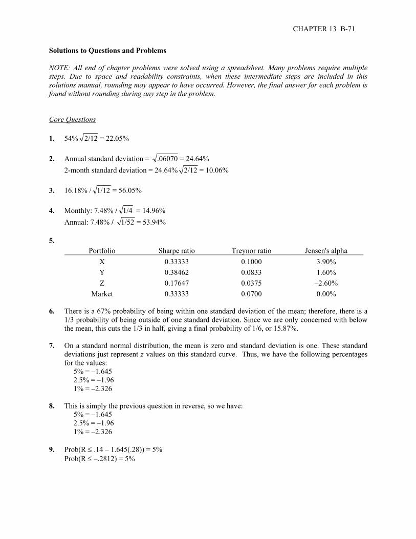
CHAPTER 13 B-71
Solutions to Questions and Problems NOTE: All end of chapter problems were solved using a spreadsheet. Many problems require multiple steps. Due to space and readability constraints, when these intermediate steps are included in this solutions manual, rounding may appear to have occurred. However, the final answer for each problem is found without rounding during any step in the problem. Core Questions 1. 54% 2/12 = 22.05% 2. Annual standard deviation = .06070 = 24.64% 2-month standard deviation = 24.64% 2/12 = 10.06% 3. 16.18% / 1/12 = 56.05% 4. Monthly: 7.48% / 1/4 = 14.96% Annual: 7.48% / 1/52 = 53.94% 5.
Portfolio Sharpe ratio Treynor ratio Jensen's alpha X 0.33333 0.1000 3.90% Y 0.38462 0.0833 1.60% Z 0.17647 0.0375 –2.60% Market 0.33333 0.0700 0.00%
6. There is a 67% probability of being within one standard deviation of the mean; therefore, there is a
1/3 probability of being outside of one standard deviation. Since we are only concerned with below the mean, this cuts the 1/3 in half, giving a final probability of 1/6, or 15.87%.
7. On a standard normal distribution, the mean is zero and standard deviation is one. These standard
deviations just represent z values on this standard curve. Thus, we have the following percentages for the values:
5% = –1.645 2.5% = –1.96 1% = –2.326 8. This is simply the previous question in reverse, so we have: 5% = –1.645 2.5% = –1.96 1% = –2.326 9. Prob(R ≤ .14 – 1.645(.28)) = 5% Prob(R ≤ –.2812) = 5%

B-72 SOLUTIONS
10. Prob(R ≤ (.16/12) – 1.96(.33)(1/12)1/2) = 2.5% Prob(R ≤ –.1734) = 2.5% 11. E(R) = (.13 + .16)/2 = .145 σ = (.52 × .252 + .52 × .332)1/2 = .2070 Prob(R ≤ (.145/12) – 1.96(.2070)(1/12)1/2) = 2.5% Prob(R ≤ –.1050) = 2.5% 12. Prob(R ≤ .15 – 2.326(.47)) = 1% Prob(R ≤ –.9434) = 1% 13. Prob(R ≤ (.18/52) – 1.96(.58)(1/52)1/2) = 2.5% Prob(R ≤ –.1542) = 2.5% 14. E(R) = (.15 + .18)/2 = .165 σ = (.52 × .472 + .52 × .582)1/2 = .3733 Prob(R ≤ (.165/12) – 1.645(.3733)(1/12)1/2) = 5% Prob(R ≤ –.1635) = 5% 15. For a portfolio with two investments having zero correlation, the Sharpe ratio would be calculated as
follows:
) x (x
R - )E(R x )E(Rx ratio Sharpe 1/22
B2B
2S
2S
fBBSS
σσ +
+=
16. ))]R,)(Corr(R)((.2(.5)(.5) .5 [.5
R - ).5E(R ).5E(R ratio Sharpe 1/2
BSBS2B
22S
2fBS
σσσσ ++
+=
17. Any portfolio of the two securities will also have the same expected return.
1/22B
2B
2S
2S
fB1/22
B2B
2S
2S
fS
) x (xR - )E(R
) x (x
R - )E(R ratio Sharpe
σσσσ +=
+=
18. Prob(R ≤ .14 – 2.326(.63)) = 1% Prob(R ≤ –1.3256) = 1% This number does not make sense since it is impossible to lose more than 100% in a stock. 19. Prob(R ≥ .14 + 2.326(.63)) = 1% Prob(R ≥ + 1.6056) = 1% While this is a large return, it is plausible, and even possible. Since it is not possible for a stock to
lose more than 100% but it is possible for a stock to gain more than 100%, stock returns are not truly normal.
20. E(R) = (.12 + .17) / 2 = .1450 σ = [(.52)(.412) + (.52)(.622) + 2(.5)(.5)(.41)(.61)(.5)]1/2 = .4491 Prob(R ≤ (.1450/12) – 1.645(.4491)(1/12)1/2) = 5% Prob(R ≤ –.2012) = 5%

CHAPTER 13 B-73
21. E(R) = (.12 + .17) / 2 = .1450 σ = [(.52)(.412) + (.52)(.622) + 2(.5)(.5)(.41)(.62)(–.5)]1/2 = .2731 Prob(R ≤ (.1450/12) – 1.645(.2731)(1/12)1/2) = 5% Prob(R ≤ –.1176) = 5% 22. E(R) = .16 σ = [(.3332)(.402) + (.3332)(.502) + (.3332)(.602) + 2(.333)(.333)(.40)(.50)(0) + 2(.333)(.333)(.40)(.60)(0) + 2(.333)(.333)(.50)(.60)(0)]1/2 = .2925 Prob(R ≤ .16 – 2.326(.2925)) = 1% Prob(R ≤ –.5205) = 1% 23. E(R) = .16 σ = [(.3332)(.402) + (.3332)(.502) + (.3332)(.602) + 2(.333)(.333)(.40)(.50)(.20) + 2(.333)(.333)(.40)(.60)(.20) + 2(.333)(.333)(.50)(.60)(.20)]1/2 = .3442 Prob(R ≤ .16 – 2.326(.3442)) = 1% Prob(R ≤ –.6406) = 1% 24. wA = [(.12 – .05)(.592) – (.16 – .05)(.34)(.59)(.20)] / {(.12 – .05)(.592) + (.16 – .05)(.342) – (.12 – .05 + .16 – .05)[(.34)(.59)(.20)]} wA = .6682 wB = .3318 E(RP) = .6682(.12) + .3318(.16) = .1333 σ = [(.66822)(.342) + (.33182)(.592) + 2(.6682)(.3318)(.34)(.59)(.20)]1/2 = .3282 Sharpe ratio = (.1333 – .05)/.3282 = .2537 Prob(R ≤ .1333 – 1.960(.3282)) = 2.5% Prob(R ≤ –.5100) = 2.5%

B-74 SOLUTIONS
Spreadsheet Problem 25. The Solver inputs are:
based on the following spreadsheet.

Chapter 14 Futures Contracts
Concept Questions 1. a. Three are visible in Figure 16.1; wheat futures are traded on the Chicago Board of Trade
(CBT), Kansas City Board of Trade (KC), and Minneapolis Grain Exchange (MPLS). There are two others, the Winnipeg Commodity Exchange (WPG) and the MidAmerica Commodity Exchange (MCE), not shown in Figure 16.1. Of these, the largest trading activity occurs in Chicago.
b. There are 100 troy oz. per contract, for a total of 1,000 troy oz. on ten contracts. It is traded on the COMEX division of the New York Mercantile Exchange.
c. At 5,000 bu. per contract, you must deliver 100,000 bushels. d. The April contract has the largest open interest and the October contract has the smallest open
interest. 2. Long hedge; i.e., buy corn futures. If corn prices do rise, then the futures position will show a profit,
offsetting the losses from higher corn prices when they are purchased. 3. Short the index futures. If the S&P 500 index subsequently declines in a market sell-off, the futures
position will show a profit, offsetting the losses on the portfolio of stocks. 4. Sell the futures. If interest rates rise, causing the value of the bonds to be less at the time of sale, the
corresponding futures hedge will show a profit. 5. Buy yen futures. If the value of the dollar depreciates relative to the yen in the intervening four
months, then the dollar/yen exchange rate will rise, and the payment required by the importer in dollars will rise. A long yen futures position would profit from the dollar's depreciation and offset the importer's higher invoice cost.
6. Sell crude oil futures. Price declines in the oil market would be offset by a gain on the short position. 7. Sell T-bond futures. Bond price declines in the market would be offset by a gain on the short
position. 8. It is true. Each contract has a buyer and a seller, a long and a short. One side can only profit at the
expense of the other. Including commissions, futures contracts, like most derivative assets, are actually negative sum gains. This doesn’t make them inappropriate tools, it just means that, on average and before commissions, they are a break-even proposition.

B-76 SOLUTIONS
9. In reality, two factors make stock index arbitrage more difficult than it might appear. First, the dividend yield on the index depends on the dividends that will be paid over the life of the contract; this is not known with complete certainty and must, therefore, be estimated. Second, buying or selling the entire index is feasible, but index staleness (discussed in our first stock market chapter) is an issue; the current up-to-the-second price of the index is not known because not all components will have just traded. Of course, trading costs must be considered as well.
Thus, there is some risk in that the inputs used to determine the correct futures price may be incorrect, and what appears to be a profitable trade may not be. Program traders usually establish bounds, meaning that no trade is undertaken unless a deviation from parity exceeds a preset amount. Setting the bounds is itself an issue. If they are set too narrow, then the risks described above exist. If they are set too wide, other traders will step in sooner and eliminate the profit opportunity.
10. There are two similarities. 1) You are selling an asset today that you do not currently own (you may
expect to own the asset in the future, say a wheat harvest). 2) Both contracts have an initial margin and a maintenance margin. There are several major differences between a futures contract and short selling a stock. 1) With a futures contract you are agreeing to a price at a specific date in the future. The price at settlement may be above or below the agreed upon price. In short selling the stock, you are selling at the current price and the price in the future is not set. 2) In a futures contract, the maturity date is determined when the contract is sold. A short stock sale can theoretically extend to infinity. 3) The cash flows from the short sale are different. In a futures contract, cash for the sale of a futures contract is not exchanged until the settlement of the contract. At the settlement date, you will receive the cash for the sale. In a short stock sale, you receive the cash for the sale of the stock today (although your broker may not allow you access to the cash). When you close the short stock position, you must pay cash to purchase the stock.
Solutions to Questions and Problems NOTE: All end of chapter problems were solved using a spreadsheet. Many problems require multiple steps. Due to space and readability constraints, when these intermediate steps are included in this solutions manual, rounding may appear to have occurred. However, the final answer for each problem is found without rounding during any step in the problem. Core Questions 1. a. The settle price is 95.40 cents per pound. One contract is valued as the contract size times the per
unit price, so 37,500 × $.09540 = $35,775.00. b. The settle price is 112:04, or 112.25% of par value. The value of a position in 10 contracts is 10 ×
$100,000 × 1.1225 = $1,121,250. c. The index futures price was up 64 for the day, or $10 × 64 = $640. For a position in 25 contracts,
this represents a change in value of 25 × 640 = $16,250, which would represent a gain to a long position in the futures contract and a loss to a short position in the futures contract.
d. The contract price closed up .03 cents for the day, so a short position would have had a loss of 10 × 60,000 × $0.0003 = $180.
2. The contract settled up 13.75 cents, so a long position gains: 20 × 5,000 × $0.0150 = $13,750. 3. The contract settled up 1.25 cents, so a short position loses: 15 × 5,000 × –$0.0125 = $937.50. 4. The contract settled up 6.5 points, so a short position loses: –30 × $100,000 × (4.5/32)% = –
$4,218.75.

CHAPTER 14 B-77
5. The total open interest on the December 2005 Japanese Yen is 132,895 contracts. This is the number of contracts. Each contract has a long and a short, so the open interest represents either the number of long positions or the number of short positions. Each contract calls for the delivery of ¥12,500,000, and the settle price on the contract is $.8342 per 100 yen, or $.8342/100 × ¥12,500,000 = $104,275.00. With 132,895 contracts, the total dollar value is about $13,857,626,125.
6. F4 = $64.87(1 + .05)4/12 = $65.93 7. $87.62 = S(1 + .045)3/12; S = $86.66 8. $33.53 = $32.17(1 + R)8/12; R = .0641 9. F4 = $74.13(1 + .054 – .015)4/12 = $75.08 10. $61.57 = S(1 + .061 – .0125)6/12; S = $60.13 Intermediate Questions 11. If the contract settles down, a long position loses money. The loss per contract is: 42,000 × $.02 =
$840, so when the account is marked-to-market and settled at the end of the trading day, your balance per contract is $660, which is less than the maintenance margin. The minimum price change for a margin call is $250 = 42,000 × X, or X = $.00595 = 0.595 cents per gallon.
12. Establish your account at an initial margin of 10 × $1,000 = $10,000. Your maintenance margin is
10 × $750 = $7,500. The initial value of the position is 10 × 100 × $480 = $480,000. Day 1: New position value = 10 × 100 × $473 = $473,000, for a loss of $7,000.
Your margin account balance is now $3,000. You must meet a margin call of $7,000, bringing your margin back to $10,000.
Day 2: New position value = 10 × 100 × $479 = $479,000, for gain of $6,000.
Your margin account balance is now $16,000. Day 3: New position value = 10 × 100 × $482 = $482,000, for a gain of $3,000.
Your margin account balance is now $19,000. Day 4: New position value = 10 × 100 × $486 = $486,000, for a gain of $4,000.
Your margin account balance is now $23,000. Your total profit is $486,000 – 480,000 = $6,000.

B-78 SOLUTIONS
13. Establish your account at an initial margin of 25 × $6,075 = $151,875. Your maintenance margin is 25 × $4,500 = $112,500. The initial value of the position is 25 × 42,000 × $1.52 = $1,596,000.
Day 1: New position value = 25 × 42,000 × $1.46 = $1,533,000, for a loss of
$63,000. Your margin account balance is $214,875, which is not below the maintenance margin level, so no margin deposit is required.
Day 2: New position value = 25 × 42,000 × $1.55 = $1,627,500, for a loss of
$94,500. Your margin account balance is now $120,375. Day 3: New position value = 25 × 42,000 × $1.59 = $1,669,500, for a loss of
$42,000. Your margin account balance is now $78,375. You must meet a margin call of $73,500, bringing your margin back to $151,875.
Day 4: New position value = 25 × 42,000 × $1.62 = $1,701,000, for a loss of
$31,500. Your margin account balance is now $120,375. Your total profit is $1,596,000 – 1,701,000 = –$105,000 14. 20 × 1,000 × ($63.69 – 58.75) = $98,800 15. –15 × 62,500 × ($1.7692 – 1.8550) = $80,437.50 16. Parity implies that F = 4,512(1 + .07 – .02)1/2 = 4,623.42. Thus, if the futures price is actually at
4,640, the futures are overpriced, and you would want to buy the index and sell the futures. 17. Since you are long in the asset (stocks), to create a hedge, you would short the futures contract. The
number of futures contracts to short is: Number of contracts = (1.15 × $300,000,000) / (740 × $500) = 923.43 or about 923 contracts. However, the Midcap 400 futures might not be liquid enough to handle such a large hedge. Also,
when the contract expires it will be necessary to “roll” the hedge into a subsequent contract month. 18. 1,253.80 = 1,231.21(1 + X)6/12; X = .0370 19. 1,274.19 = 1,241.71(1 + .07 – d)1/2; d = .0170 20. DF = 8.5 + (3/12) = 8.75 years Contracts to sell = (5.1 × $900,000,000) / (8.75 × 1.03 × $100,000) = 5,092.93 or about 5,093
contracts. 21. DF = 8 + (85/365) = 8.23 years Contracts to sell = (11.2 × $400,000,000) / (8.23 × 1.02 × $100,000) = 5,334.90 or about 5,335
contracts.

CHAPTER 14 B-79
22. F = $87.12(1 + .04)5/12 = $88.56; the futures is underpriced Opening transactions now: Buy the futures $0 Sell the stock –$87.12 Lend $87.12 at 4% for 5 months +$87.12 Total cash flow $0.00 Closing transactions: Accept delivery on the futures –$88.38 Cover the short position $0 Collect the loan +$88.56 Total cash flow $0.18 23. F = $92.12(1 + .04)5/12 = $95.29; the futures is overpriced Opening transactions now: Sell the futures $0 Buy the stock –$92.12 Borrow $92.12 at 7% for 6 months +$92.12 Total cash flow $0.00 Closing transactions: Deliver the futures +$95.87 Sell the stock $0 Repay the loan –$95.29 Total cash flow $0.58 24. AIMR suggested answers: a. The arbitrage strategy that would take advantage of the arbitrage opportunity is a Reverse Cash
and Carry. A Reverse Cash and Carry opportunity results from the following relationship not holding true:
F0,t ≥ S0 (1 + C) If the futures price is less than the spot price plus the cost of carrying the goods to the futures
delivery date, and arbitrage in the form of a Reverse Cash and Carry exists. A trader would be able to sell the asset short, use the proceeds to lend at the prevailing interest rate, and buy the asset for future delivery. At the future delivery, the trader would then collect the proceeds from the loan with interest, accept delivery of the asset, and cover the short position with the commodity.
b. Opening transactions now: Sell the commodity short +$120.00 Buy the commodity futures expiring in 1 year 0.00 Contract to lend $120 at 8% for 1 year –$120.00 Total cash flow $0.00 Closing transactions one year from now: Accept delivery on expiring futures –$125.00 Cover the short commodity position 0.00 Collect on loan of $120 +$129.60 Total cash flow $4.60
B-80 SOLUTIONS
c. Direct Transaction Costs: First, the trader must pay a fee to have an order executed. This fee includes commissions and various exchange fees. Second, in every market, there is a bid-ask spread. Market makers on the floor of the exchange must try to sell at a higher price (ask price) than the price at which they are willing to buy (bid price). Without the inclusion of transactions costs, the same arbitrage opportunity that is profitable without transaction costs may not be profitable after transaction costs. Rather than having a specific no-arbitrage price in which traders can profit, there is now a bond of no-arbitrage futures prices, bounded by the applicable transaction costs.
Unequal Borrowing and Lending Rates: In perfect markets, all traders can borrow and lend at the risk-free rate. This is not true in real markets. Generally, traders face a borrowing rate that exceeds the lending rate. As in the case of transaction costs, There is no longer a single no-arbitrage price but rather a transaction that has boundaries established by the differential between the borrowing and lending rates.
Restrictions on Short Selling: In perfect markets traders can sell assets short and use the proceeds from the short sale. In actual markets, however, there are serious impediments to short selling. First, for some goods, there is virtually no opportunity for short selling. This is particularly true for many physical goods. Second, even when short selling is permitted, restrictions limit the use of funds from the short sale. Often these restrictions mean that the short seller does not have the use of all of the proceeds from the short sale. This particularly is important in the reverse cash and carry, where the short sale is employed in the transaction. Short selling restrictions lower the boundary of the reverse cash and carry. If an investor can only use a portion of the short sale proceeds, that condition will depress the lower boundary, having little effect on the futures price.
Limitations on Storage: The storability of a commodity is important in the futures pricing of some commodities. While some goods store well, others do not. Perishable commodities are said to have infinite storage costs. This limitation to storage means that a cash and carry strategy cannot link futures and cash prices. Therefore, when the cash and carry or reverse cash and carry strategy are executed, the inability to store a commodity indefinitely can cause the no arbitrage bounds to be altered to reflect the actual limitations to storage.
Supply Shortage: The supple of commodities such as gold is large relative to its consumption, hence the market for gold will closely approximate its full carry market. The supply of some industrial metals is small relative to consumption and those markets are not full carry markets.
Seasonal Factors: Highly seasonal production or consumption factors can cause distortions in normal price relationships.
Tam must also realize that these imperfections differ widely across markets and have different
effects on different traders, and that their potential effect on her ability to implement a given arbitrage strategy depends on her unique circumstances.

CHAPTER 14 B-81
25. AIMR suggested answers: a. According to the cost-of-carry rule, the futures price must equal the spot price plus the cost of
carrying the spot commodity forward to the delivery date of the futures contract. F0,6 = 185.00 × (1 + .06/2) = 190.55 b. Assuming that the only carrying charge is the financing cost at an interest rate of 6.00 percent,
the lower bound imposed by the reverse cash-and-carry strategy including transaction costs is: Cash inflows: - Buy 1 contract of TOBEC stock index futures (December contract) - Sell the index spot at 185.00 × $100 = $18,500 - Invest the proceeds at the risk-free rate for six months (until the expiration of the contract) $18,500 × (1 + .06/2) = $19,055 Six months from now: At expiration the futures price is assumed to converge to the spot price, and - Sell 1 contract of the TOBEC stock index futures (December contract) - Buy the index spot - Collect on the investment ($19,055) - Pay transaction costs = $15.00 Total = $19,055 – 15.00 = $19,040 Lower bound = $19,040 / $100 = 190.40

Chapter 15 Stock Options
Concept Questions 1. Assuming American-style exercise rights, a call option confers the right, without the obligation, to
buy an asset at a given price on or before a given date. An American-style put option confers the right, without the obligation, to sell an asset at a given price on or before a given date. European-style options are the same except that exercise can only occur at maturity. One reason you would buy a call option is that you expect the price of the asset to increase. Similarly, you would buy a put option if you expect the price of the asset to decrease. In both cases, other reasons exist, but these are the basic ones. A call option has unlimited potential profit, while a put option has limited potential profit; the underlying asset's price cannot be less than zero.
2. a. The buyer of a call option pays money for the right to buy....
b. The buyer of a put option pays money for the right to sell.... c. The seller of a call option receives money for the obligation to sell.... d. The seller of a put option receives money for the obligation to buy....
3. In general, the breakeven stock price for a call purchase is the exercise price plus the premium paid.
For stock prices higher than this, the purchaser realizes a profit. For a put purchase, it’s the strike price less the premium. For stock prices lower than this, the purchaser realizes a profit.
4. If you buy a put option on a stock that you already own, you guarantee that you can sell the stock for
the strike price on the put. Thus, you have, in effect, insured yourself against stock price declines beyond this point. This is the protective put strategy.
5. The intrinsic value of a call option is max{0, S – K}. It is the value of the option if it were exercised
immediately. 6. The intrinsic value of a put option at expiration is max{0, K – S}. By definition, the intrinsic value
of an option is its value if it were exercised immediately. 7. The call is selling for less than its intrinsic value; an arbitrage opportunity exists. Buy the call for
$10, exercise the call by paying $35 in return for a share of stock, and sell the stock for $50. You've made a riskless $5 profit.
8. 42 contracts were traded, 25 calls and 17 puts; this represents options on 4,200 shares of Milson
stock. 9. The calls are in the money. The intrinsic value of the calls is $4. 10. The puts are out of the money. The intrinsic value of the puts is $0.
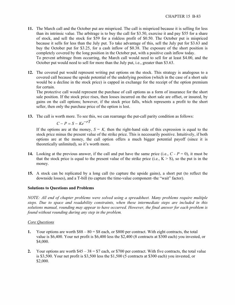
CHAPTER 15 B-83
11. The March call and the October put are mispriced. The call is mispriced because it is selling for less than its intrinsic value. The arbitrage is to buy the call for $3.50, exercise it and pay $55 for a share of stock, and sell the stock for $59 for a riskless profit of $0.50. The October put is mispriced because it sells for less than the July put. To take advantage of this, sell the July put for $3.63 and buy the October put for $3.25, for a cash inflow of $0.38. The exposure of the short position is completely covered by the long position in the October put, with a positive cash inflow today.
To prevent arbitrage from occurring, the March call would need to sell for at least $4.00, and the October put would need to sell for more than the July put, i.e., greater than $3.63.
12. The covered put would represent writing put options on the stock. This strategy is analogous to a
covered call because the upside potential of the underlying position (which in the case of a short sale would be a decline in the stock price) is capped in exchange for the receipt of the option premium for certain.
The protective call would represent the purchase of call options as a form of insurance for the short sale position. If the stock price rises, then losses incurred on the short sale are offset, or insured, by gains on the call options; however, if the stock price falls, which represents a profit to the short seller, then only the purchase price of the option is lost.
13. The call is worth more. To see this, we can rearrange the put-call parity condition as follows:
C P S Ke rT− = − − If the options are at the money, S = K, then the right-hand side of this expression is equal to the
stock price minus the present value of the strike price. This is necessarily positive. Intuitively, if both options are at the money, the call option offers a much bigger potential payoff (since it is theoretically unlimited), so it’s worth more.
14. Looking at the previous answer, if the call and put have the same price (i.e., C - P = 0), it must be
that the stock price is equal to the present value of the strike price (i.e., K > S), so the put is in the money.
15. A stock can be replicated by a long call (to capture the upside gains), a short put (to reflect the
downside losses), and a T-bill (to capture the time-value component–the “wait” factor). Solutions to Questions and Problems NOTE: All end of chapter problems were solved using a spreadsheet. Many problems require multiple steps. Due to space and readability constraints, when these intermediate steps are included in this solutions manual, rounding may appear to have occurred. However, the final answer for each problem is found without rounding during any step in the problem. Core Questions 1. Your options are worth $88 – 80 = $8 each, or $800 per contract. With eight contracts, the total
value is $6,400. Your net profit is $6,400 less the $2,400 (8 contracts at $300 each) you invested, or $4,000.
2. Your options are worth $45 – 38 = $7 each, or $700 per contract. With five contracts, the total value
is $3,500. Your net profit is $3,500 less the $1,500 (5 contracts at $300 each) you invested, or $2,000.

B-84 SOLUTIONS
3. The stock costs $80 per share, so if you invest $12,000, you’ll get 150 shares. The option premium is $3, so an option contract costs $300. If you invest $12,000, you’ll get $12,000/$300 = 40 contracts. If the stock is selling for $90 in 90 days, your profit on the stock is $10 per share, or $1,500 total. The percentage gain is $1,500/$12,000 = 12.50%. Your options are worth $10 per share, or $1,000 per contract. However, you have 40 contracts, so your options are worth $40,000 in all. Since you paid $12,000 for the 40 contracts, your profit is $28,000. Your percentage gain is a pleasant $28,000/$12,000 = 233.33%.
If the stock is selling for $80, your profit is $0 on the stock, so your percentage return is 0%. Your option is worthless (why?); the percentage loss is –100%. If the stock is selling for $70, verify that your percentage loss on the stock is –12.50% and your loss on the option is again –100%.
4. 50 contracts at $670 per contract = $33,500 5. Stock price = $84: option value = 50(100)($84 – 70) = $70,000 Stock price = $75: option value = 50(100)($75 – 70) = $25,000 6. Initial cost = 30(100)($3.90) = $11,700; maximum gain = 30(100)($70) – 11,700 = $198,300.
Terminal value = 30(100)($63 – 70) = $21,000; net gain = $21,000 – 11,700 = $9,300 7. Stock price = $55: net loss = $11,700 – 45,000 = –$33,300. Stock price = $100: net gain = $11,700. The breakeven stock price is the $70 exercise price less the premium of $3.90, or $66.10. For
terminal stock prices above $66.10, the premium received more than offsets any loss, so the writer of the put option makes a net profit (ignoring commissions and the effects of the time value of money).
8. P = C – S + Ke–rT
P = $6 – $61 + $60e–.05(.5) P = $8.40 9. S = C – P + Ke–rT
S = $8 – $4 + $80e–.04(.5) S = $82.42 10. C = S + P – Ke–rT
C = $78 + $8.90 – $75e–.05(2/12) C = $12.52 Intermediate Questions 11. P = C – Se–yT + Ke–rT
P = $9.40 – $58e–.02(5/12) + $55e–.05(5/12) P = $5.75 12. S = (C – P + Ke–rT) / e–yT S = ($3.80 – $7.10 + $70e–.06(3/12)) / e–.03(3/12)
S = $66.15 13. C = Se–yT + P – Ke–rT
C = $83e–.02(7/12) + $6.20 – $80e–.05(7/12) C = $10.54

CHAPTER 15 B-85
14. You get to keep the premium in all cases. For 20 contracts and a $3.50 premium, that’s $7,000. If the stock price is $40 or $50, the options expire worthless, so your net profit is $7,000. If the stock price is $60, you lose $10 per share on each of 2,000 shares, or $20,000 in all. You still have the premium, so your net loss is $13,000.
15. You get to keep the premium in all cases. For 15 contracts and a $2.40 premium, that’s $3,600. If the
stock price is $35 or $45, the options expire worthless, so your net profit is $3,600. If the stock price is $25, you lose $10 per share on each of 1,500 shares, or $15,000 in all. You still have the premium, so your net loss is $11,400.
16. The contract costs $2,100. At maturity, an in-the-money SPX option is worth 100 times the
difference between the S&P index and the strike, or $4,000 in this case. Your net profit is $1,900. 17.
Stock price
Short profit Covered put
payoff Short
put profit
Net profit $60 $10 –$10 –$6.50 $3.50 $65 $5 –$5 –$1.50 $3.50 $70 $0 $0 $3.50 $3.50 $75 –$5 $0 $3.50 –$1.50 $80 –$10 $0 $3.50 –$6.50 18.
Stock price
Short profit Protective call payoff
Protective call profit
Net profit
$60 $10 $0 –$5.20 $4.80 $65 $5 $0 –$5.20 –$0.20 $70 $0 $0 –$5.20 –$5.20 $75 –$5 $5 –$0.20 –$5.20 $80 –$10 $10 $4.80 –$5.20 19.
Stock price
Short profit Covered put
payoff Protective call payoff
Total payoff
$60 $10 –$10 $0 $0 $65 $5 –$5 $0 $0 $70 $0 $0 $0 $0 $75 –$5 $0 $5 $0 $80 –$10 $0 $10 $0 20. Stock price Put payoff Call payoff Total payoff $60 –$10 $0 –$10 $65 –$5 $0 –$5 $70 $0 $0 $0 $75 $0 $5 $5 $80 $0 $10 $10
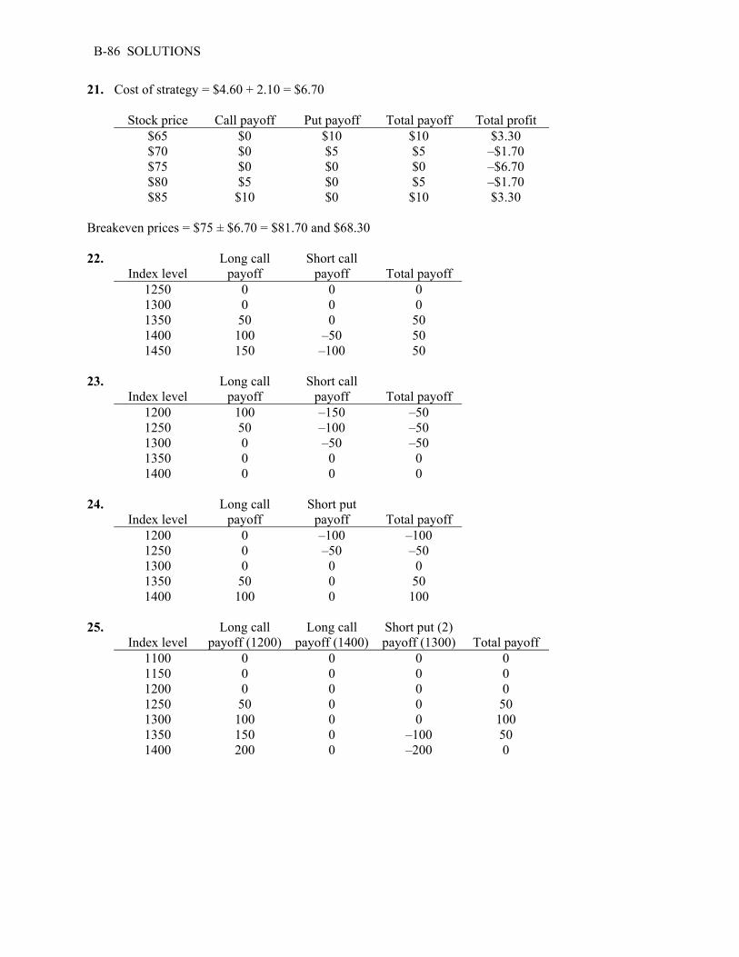
B-86 SOLUTIONS
21. Cost of strategy = $4.60 + 2.10 = $6.70 Stock price Call payoff Put payoff Total payoff Total profit $65 $0 $10 $10 $3.30 $70 $0 $5 $5 –$1.70 $75 $0 $0 $0 –$6.70 $80 $5 $0 $5 –$1.70 $85 $10 $0 $10 $3.30 Breakeven prices = $75 ± $6.70 = $81.70 and $68.30 22.
Index level Long call
payoff Short call
payoff
Total payoff 1250 0 0 0 1300 0 0 0 1350 50 0 50 1400 100 –50 50 1450 150 –100 50 23.
Index level Long call
payoff Short call
payoff
Total payoff 1200 100 –150 –50 1250 50 –100 –50 1300 0 –50 –50 1350 0 0 0 1400 0 0 0 24.
Index level Long call
payoff Short put
payoff
Total payoff 1200 0 –100 –100 1250 0 –50 –50 1300 0 0 0 1350 50 0 50 1400 100 0 100 25.
Index level Long call
payoff (1200) Long call
payoff (1400) Short put (2) payoff (1300)
Total payoff
1100 0 0 0 0 1150 0 0 0 0 1200 0 0 0 0 1250 50 0 0 50 1300 100 0 0 100 1350 150 0 –100 50 1400 200 0 –200 0

Chapter 16 Option Valuation
Concept Questions 1. The six factors are the stock price, the strike price, the time to expiration, the risk-free interest rate,
the stock price volatility, and the dividend yield. 2. Increasing the time to expiration increases the value of an option. The reason is that the option gives
the holder the right to buy or sell. The longer the holder has that right, the more time there is for the option to increase in value. For example, imagine an out-of-the-money option that is about to expire. Because the option is essentially worthless, increasing the time to expiration obviously would increase its value.
3. An increase in volatility acts to increase both put and call values because greater volatility increases
the possibility of favorable in-the-money payoffs. 4. An increase in dividend yields reduces call values and increases put values. The reason is that, all
else the same, dividend payments decrease stock prices. To give an extreme example, consider a company that sells all its assets, pays off its debts, and then pays out the remaining cash in a final, liquidating dividend. The stock price would fall to zero, which is great for put holders, but not so great for call holders.
5. Interest rate increases are good for calls and bad for puts. The reason is that if a call is exercised in
the future, we have to pay a fixed amount at that time. The higher the interest rate, the lower is the present value of that fixed amount. The reverse is true for puts in that we receive a fixed amount.
6. The time value of both a call option and a put option is the difference between the price of the option
and the intrinsic value. For both types of options, as maturity increases, the time value increases since you have a longer time to realize a price increase (decrease). A call option is more sensitive to the maturity of the contract.
7. An option’s delta tells us the (approximate) dollar change in the option’s value that will result from a
change in the stock price. If a call sells for $5.00 with a delta of .60, a $1 stock price increase will add $.60 to the option price, increasing it to $5.60.
8. The delta relates dollar changes in the stock to dollar changes in the option. The eta relates
percentage changes. So, if the stock price rises by 4 percent ($100 to $104), an eta of 10 implies that the option price will rise by 40 percent.
9. Vega relates the change in volatility in percentage points to the dollar change in the option’s price. If
volatility rises from 40 to 41 percent, a 1 point rise, and vega is .80, then the option’s price will rise by 80 cents.
10. Rho measures option price sensitivity to a change in the interest rate, where a 1 percent change in the
interest rate causes the option price to change by approximately the amount rho. If the interest rate rises from 4 percent to 5 percent (a 1 percent increase), the call price will increase by $.14 from $10.00 to $10.14.
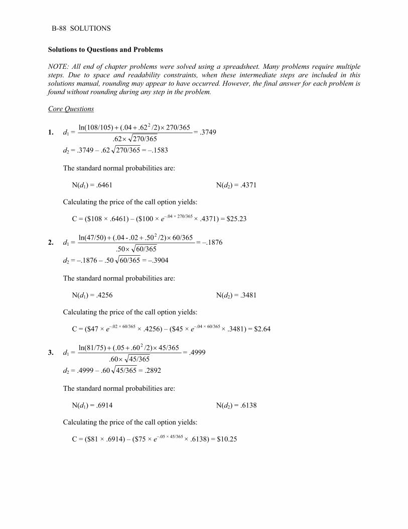
B-88 SOLUTIONS
Solutions to Questions and Problems NOTE: All end of chapter problems were solved using a spreadsheet. Many problems require multiple steps. Due to space and readability constraints, when these intermediate steps are included in this solutions manual, rounding may appear to have occurred. However, the final answer for each problem is found without rounding during any step in the problem. Core Questions
1. d1 = 270/365 .62
270/365 /2).62 (.04 )ln(108/105 2
×
×++ = .3749
d2 = .3749 – .62 270/365 = –.1583 The standard normal probabilities are: N(d1) = .6461 N(d2) = .4371 Calculating the price of the call option yields: C = ($108 × .6461) – ($100 × e–.04 × 270/365 × .4371) = $25.23
2. d1 = 60/365 .50
60/365 /2).50 .02 - (.04 ln(47/50) 2
×
×++ = –.1876
d2 = –.1876 – .50 60/365 = –.3904 The standard normal probabilities are: N(d1) = .4256 N(d2) = .3481 Calculating the price of the call option yields: C = ($47 × e–.02 × 60/365 × .4256) – ($45 × e–.04 × 60/365 × .3481) = $2.64
3. d1 = 45/365 .60
45/365 /2).60 (.05 ln(81/75) 2
×
×++ = .4999
d2 = .4999 – .60 45/365 = .2892 The standard normal probabilities are: N(d1) = .6914 N(d2) = .6138 Calculating the price of the call option yields: C = ($81 × .6914) – ($75 × e–.05 × 45/365 × .6138) = $10.25
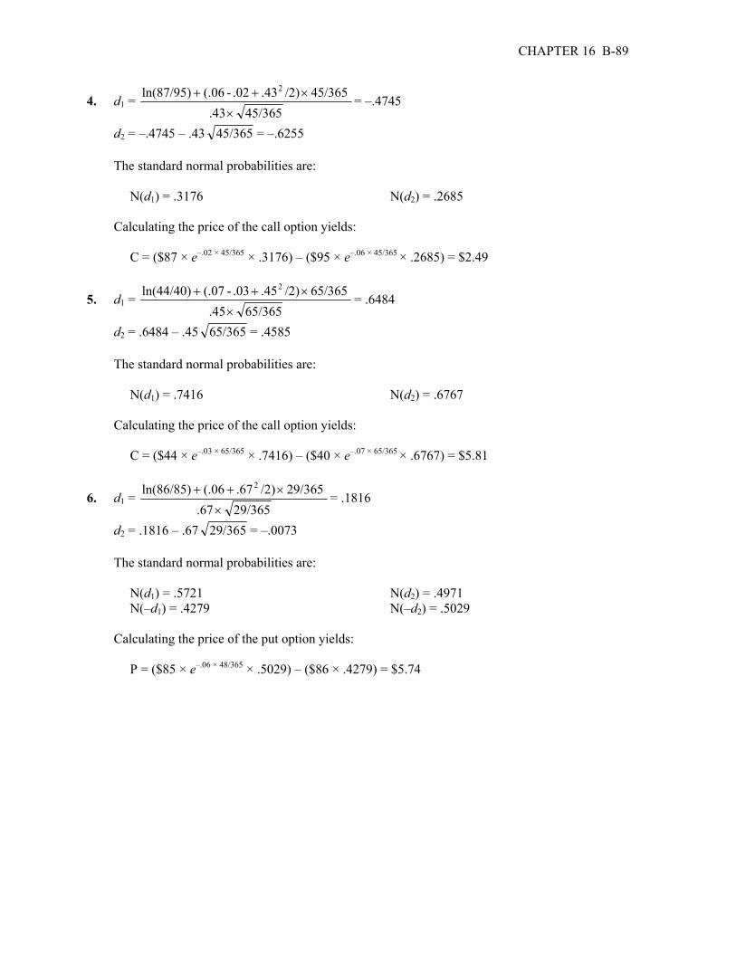
CHAPTER 16 B-89
4. d1 = 45/365 .43
45/365 /2).43 .02 - (.06 ln(87/95) 2
×
×++ = –.4745
d2 = –.4745 – .43 45/365 = –.6255 The standard normal probabilities are: N(d1) = .3176 N(d2) = .2685 Calculating the price of the call option yields: C = ($87 × e–.02 × 45/365 × .3176) – ($95 × e–.06 × 45/365 × .2685) = $2.49
5. d1 = 65/365 .45
65/365 /2).45 .03 - (.07 ln(44/40) 2
×
×++ = .6484
d2 = .6484 – .45 65/365 = .4585 The standard normal probabilities are: N(d1) = .7416 N(d2) = .6767 Calculating the price of the call option yields: C = ($44 × e–.03 × 65/365 × .7416) – ($40 × e–.07 × 65/365 × .6767) = $5.81
6. d1 = 29/365 .67
29/365 /2).67 (.06 ln(86/85) 2
×
×++ = .1816
d2 = .1816 – .67 29/365 = –.0073 The standard normal probabilities are: N(d1) = .5721 N(d2) = .4971 N(–d1) = .4279 N(–d2) = .5029 Calculating the price of the put option yields: P = ($85 × e–.06 × 48/365 × .5029) – ($86 × .4279) = $5.74
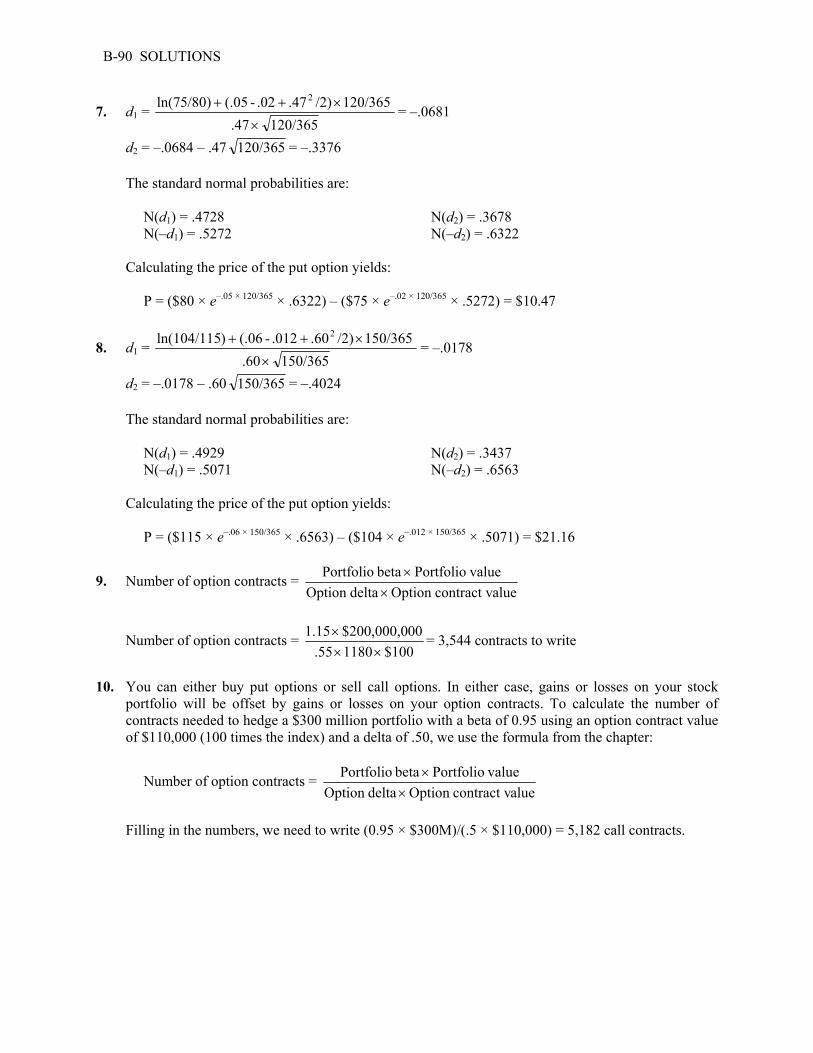
B-90 SOLUTIONS
7. d1 = 120/365 .47
120/365 /2).47 .02 - (.05 ln(75/80) 2
×
×++ = –.0681
d2 = –.0684 – .47 120/365 = –.3376 The standard normal probabilities are: N(d1) = .4728 N(d2) = .3678 N(–d1) = .5272 N(–d2) = .6322 Calculating the price of the put option yields: P = ($80 × e–.05 × 120/365 × .6322) – ($75 × e–.02 × 120/365 × .5272) = $10.47
8. d1 = 150/365 .60
150/365 /2).60 .012 - (.06 )ln(104/115 2
×
×++ = –.0178
d2 = –.0178 – .60 150/365 = –.4024 The standard normal probabilities are: N(d1) = .4929 N(d2) = .3437 N(–d1) = .5071 N(–d2) = .6563 Calculating the price of the put option yields: P = ($115 × e–.06 × 150/365 × .6563) – ($104 × e–.012 × 150/365 × .5071) = $21.16
9. Number of option contracts = aluecontract vOption deltaOption
valuePortfolio beta Portfolio×
×
Number of option contracts = $100 1180 .55
00$200,000,0 1.15××
× = 3,544 contracts to write
10. You can either buy put options or sell call options. In either case, gains or losses on your stock
portfolio will be offset by gains or losses on your option contracts. To calculate the number of contracts needed to hedge a $300 million portfolio with a beta of 0.95 using an option contract value of $110,000 (100 times the index) and a delta of .50, we use the formula from the chapter:
Number of option contracts = aluecontract vOption deltaOption
valuePortfolio beta Portfolio×
×
Filling in the numbers, we need to write (0.95 × $300M)/(.5 × $110,000) = 5,182 call contracts.
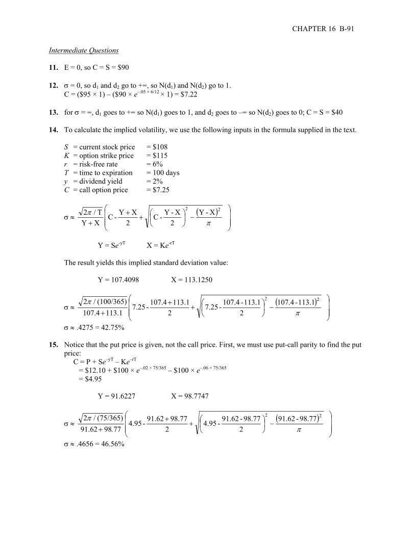
CHAPTER 16 B-91
Intermediate Questions 11. E = 0, so C = S = $90 12. σ = 0, so d1 and d2 go to +∞, so N(d1) and N(d2) go to 1. C = ($95 × 1) – ($90 × e–.05 × 6/12 × 1) = $7.22 13. for σ = ∞, d1 goes to +∞ so N(d1) goes to 1, and d2 goes to –∞ so N(d2) goes to 0; C = S = $40 14. To calculate the implied volatility, we use the following inputs in the formula supplied in the text. S = current stock price = $108 K = option strike price = $115 r = risk-free rate = 6% T = time to expiration = 100 days y = dividend yield = 2% C = call option price = $7.25
σ ≈ ( ) X - Y 2
X - Y - C 2
X Y - CX YT / 2 22
−
+
++ ππ
Y = Se-yT X = Ke-rT The result yields this implied standard deviation value: Y = 107.4098 X = 113.1250
σ ≈ ( ) 113.1 - 107.4 2
113.1 -107.4 - 7.25 2
113.1 107.4 - 7.25113.1 107.4
(100/365) / 2 22
−
+
++ π
π
σ ≈ .4275 = 42.75% 15. Notice that the put price is given, not the call price. First, we must use put-call parity to find the put
price: C = P + Se–yT – Ke–rT = $12.10 + $100 × e–.02 × 75/365 – $100 × e–.06 × 75/365 = $4.95 Y = 91.6227 X = 98.7747
σ ≈ ( ) 98.77 - 91.62 2
98.77 -91.62 -4.95 2
98.77 91.62 - 4.957798 91.62
(75/365) / 2 22
−
+
++ π
π.
σ ≈ .4656 = 46.56%

B-92 SOLUTIONS
16. d1 = 60/365 .50
(60/365) /2).50 .015 - (.05 ln(82/90) 2
×
×++ = –.3295
d2 = –.3295 – .50 60/365 = –.5322 The standard normal probabilities are: N(d1) = .3709 N(d2) = .2973 N(–d1) = .6291 N(–d2) = .7027 The option prices are: C = ($82 × e–.015 × 60/365 × .3709) – ($90 × e–.05 × 60/365 × .2973) = $3.80 P = ($90 × e–.05 × 60/365 × .7027) – ($93 × e–.015 × 60/365 × .6291) = $11.27 Option deltas are then calculated as: Call option Delta = e–yTN(d1) = e–.015 × 60/365 × .3709 = .3700 Put option Delta = –e–yTN(–d1) = –e–.015 × 60/365 × .6291 = –.6275 Option etas are calculated as: Call option Eta = e–yTN(d1)S/C = .3700 × $82/$3.80 = 7.9814 Put option Eta = –e–yTN(–d1)S/P = –.6275 × $82/$11.27 = –4.5674 For the call and put option vega, we first compute the standard normal density value for d1 as:
n(d1) = 2
e /2-d21
π=
π2
21376 /.e− = .3779
and then compute vega as Vega = Se-yTn(d1)( T ) = 82 × e–.015 × 60/365 × .3779 × 36560 / = 12.5318
17. d1 = 3.8 .36
3.8 /2).36 (.0289 9.70)ln(41.06/2 2
×
×++ = 0.9689
d2 = 0.9689 – .36 3.8 = 0.2671 These standard normal probabilities are given: N(d1) = .8337 N(d2) = .6053 Calculating the price of the employee stock options yields: ESO = ($41.06 × .9689) – ($29.70 × e–.0289 × 3.8 × .6053) ESO = $18.12

CHAPTER 16 B-93
18. This is a hedging problem in which you wish to hedge one option position with another. Your employee stock option (ESO) position represents 10,000 shares, and you need to know how many put option contracts are required to establish the hedge. First, we need to calculate deltas for both options.
Using values from the previous answer, the ESO delta is ESO (Call) Delta = e–yTN(d1) = e–0(3.8) × .9689 = .9689 For the put option, we this value for d1
d1 = .25 .36
.25 /2).36 (.0289 5)ln(41.06/4 2
×
×++ = –.3789
These standard normal probabilities are given: N(d1) = .3524 N(–d1) = .6476 Put option Delta = –e–yTN(–d1) = –1 × .6476 = –.6476 The number of put option contracts is then calculated as
Number of option contracts = 100 deltaoption Put
10,000 delta ESO×
× = 100 .6476-
10,000 .8337×
×
Performing the calculation and ignoring the minus sign yields 128.73, or about 129, put option
contracts. 19. After the volatility shift, we need to recalculate deltas for both options. The new value of d1 for the ESO is:
d1 = 3.8 .45
3.8 /2).45 .00 - (.0289 9.70)ln(41.06/2 2
×
×++ = 0.9330
In turn, the new ESO delta is ESO (Call) Delta = e-yTN(d1) = 1 × .8246 = .8246 For the put option, we obtain this value for d1
d1 = .25 .45
.25 /2).45 .00 - (.0289 5)ln(41.06/4 2
×
×++ = –.2626
and this put option delta Put option Delta = –e–yTN(–d1) = –1 × .6036 = –.6036
B-94 SOLUTIONS
The new number of contracts required is:
Number of option contracts = 1006036000108246
×−×
.,.
Which yields (ignoring the minus sign) 136.62, or about 137, put option contracts. 20. First, using put-call parity we calculate the corresponding call option price. C = P + Se–yT – Ke–rT
C = $6.00 + $41.06e–.00(.25) – $45e–.0289(.25) C = $2.38 Y = 41.0600 X = 44.6760
σ ≈ ( ) X - Y 2
X - Y - C 2
X Y - CX YT / 2 22
−
+
++ ππ
σ ≈ ( ) 44.68 - 41.06 244.687 -41.06 -2.38
244.68 41.06 - 2.38
6844 41.06(.25) / 2 22
−
+
++ π
π.
σ ≈ .4592 or 45.92% AIMR suggested answers: 21. Donie should choose the long strangle. A long strangle consists of buying a put and a call with the
same expiration date and the same underlying asset. In a strangle strategy, the call has an exercise price above the stock price and the put has an exercise price below the stock price. An investor who buys (goes long) a strangle expects that the price of the underlying asset (TRT in this case) will either move substantially below the exercise price on the put or above the exercise price on the call. With respect to TRT, the long strangle investor buys both the put and call options for a total cost of $9.00, and will experience large profits of the stock moves more than $9.00 above the call exercise price of $9.00 below the put exercise price. This strategy would enable Donie’s client to profit from a large move in stock price, either up or down, in reaction to the court decision.
22. The maximum possible loss per share is $9.00, which is the total cost of the two options = $5.00 +
$4.00. The maximum possible gain is unlimited if the stock price moves above the call strike price. The breakeven prices are $46.00 and $69.00. The put will just cover costs if the stock price finishes $9.00 below the put exercise price ($55.00 – 9.00 = $46.00), and the call will just cover costs of the stock price finishes $9.00 above the call exercise price ($60.00 + 9.00 = $69.00).
23. The delta for a call option is always positive, so the value of the call option will increase if the stock
price increases. Specifically, if the stock price increases by $1.00, the price of the call will increase by approximately $0.63:
Change in call price = (0.6250 × $1.00) = $0.625 increase.

CHAPTER 16 B-95
Spreadsheet Answers
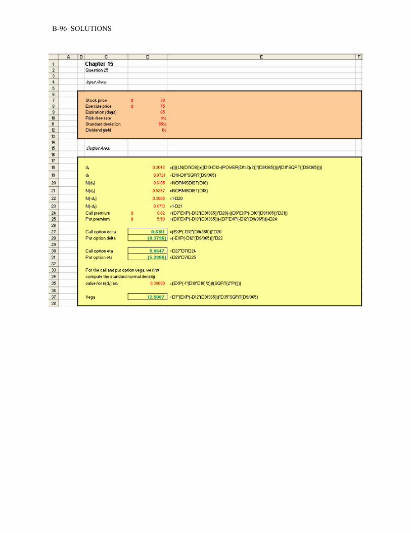
B-96 SOLUTIONS
Chapter 17
Projecting Cash Flow and Earnings Concept Questions 1. The 10K and 10Q are reports public firms must file with the SEC. They contain, among other things,
financial statements including balance sheets, income statements, and cash flow statements. The easiest way to retrieve them is on-line from EDGAR.
2. The reason is that, ultimately, sales are the driving force behind a business. A firm’s assets,
employees, and, in fact, just about every aspect of its operations and financing exist to directly or indirectly support sales. Put differently, a firm’s future need for things like capital assets, employees, inventory, and financing are determined by its future sales level.
3. They are current in the sense that they are expected to convert to cash (or otherwise be used up)
within the next 12 months. Operating assets are current because they simply consist of current assets other than cash.
4. Earnings per share are equal to net income divided by the number of shares outstanding. Net income
is sometimes called “total earnings.” There are some issues concerning how to measure shares outstanding, but these go beyond the scope of this chapter.
5. Depreciation is a “noncash item” because the depreciation deduction does not literally represent a
cash outflow. It is instead purely an accounting entry. 6. Operating cash flow, investing cash flow, and financing cash flow. 7. It is the cash generated by ordinary business activity, meaning the everyday, routine functioning of
the business. 8. ROE is a better measure of the company’s performance. ROE shows the percentage return for the
year earned on shareholder investment. Since the goal of a company is to maximize shareholder wealth, this ratio shows the company’s performance in achieving this goal over the period.
9. The retained earnings number on the income statement is the amount retained that year. The number
on the balance sheet is the cumulative amount from all previous years. Put differently, the income statement number is the increment or addition to the balance sheet number.
10. Gross margin is gross profit divided by sales, where gross profit is sales less cost of goods sold.
Operating margin is operating profit divided by sales, where operating profit is equal to gross profit less operating expenses. Thus, the difference is that operating margin considers both costs of goods sold and operating expenses. They indicate how much of each sales dollar is left after accounting for costs of goods sold (gross margin) and, additionally, for operating expenses (operating margin). Generally speaking, larger values are better.
11. Gross margin will be larger (why?). Both can be negative. Also, gross margin can be positive while
operating margin is negative, but not the other way around (why?).
B-98 SOLUTIONS
12. No, but dividend paying companies certainly wish they were! Dividends received from another company are taxed preferentially. Depending on the circumstances, only 20 percent or 30 percent are subject to taxes; the rest is not taxed.
13. The bottom line on the cash flow statement is operating cash flow, less money spent on fixed assets
and other investments, less the net amount paid or raised due to financial transactions (i.e., things like borrowing money, paying dividends, or paying interest). It actually measures the change in the amount of cash the firm has available from one period to the next.
14. The literal interpretation is that it is the sum of all the yearly retained earnings numbers. There are
two important things to recognize. First, in any given year, the retained earnings number on the income statement is simply what’s left over after dividends are subtracted from net income. Dividends are paid in cash, but net income is not a cash flow (because, for example, it includes noncash deductions). As a result, the retained earnings are not cash flows either. The actual cash flow that is “retained” is some very different number. Second, to the extent that Coors does “retain” cash, that cash doesn’t just sit there. Instead, it is used to do things like purchase assets and pay off debts. Cash or earnings aren’t so much “retained” as they are “reinvested.” Thus, the retained earnings number isn’t cash, and even if it were, it wouldn’t just be a pile of cash sitting around somewhere.
15. AIMR suggested answer: For companies in the industry described, the price-to-sales ratio would be superior to either of the
other two ratios because the price-to-sales ratio is: - More useful in valuing companies with negative earnings or negative book values (a frequent
consequence of rapid technological change) - Better able to compare companies in different countries that are likely to be using different
accounting methods, i.e., standards (a consequence of the multinational nature of the industry) - Less subject to manipulation, i.e., managing earnings by management (a frequent consequence
when firms are in a cyclical low and likely to report losses) - Not as volatile as PE multiples and hence may be more reliable for use in valuation - Less subject to distortion from currency translation effects - Less influenced by accounting values in the presence of rapid technological changes

CHAPTER 17 B-99
Core Questions NOTE: All end of chapter problems were solved using a spreadsheet. Many problems require multiple steps. Due to space and readability constraints, when these intermediate steps are included in this solutions manual, rounding may appear to have occurred. However, the final answer for each problem is found without rounding during any step in the problem. 1. Sales $234,000 Cost of goods sold 135,000 Gross profit $ 99,000 Operating expense 53,000 Operating income $ 46,000 Investment income 2,100 Investment expense 4,600 Pretax income $ 43,500 Income taxes 15,225 Net income $ 28,275 Dividends $ 5,800 Retained earnings $22,475
2. Cash $ 26,000 Current liabilities $ 29,000 Operating assets 69,000 Long-term debt 87,000 Fixed assets 125,000 Other liabilities 9,000 Investments 26,000 Other assets 27,000 Stockholder equity 148,000 Total assets $ 273,000 Total liabilities and equity $ 273,000
3. Gross margin = $99,000/$234,000 = 42.31% Operating margin = $46,000/$234,000 = 19.66% ROA = $28,275/$273,000 = 10.36% ROE = $28,275/$148,000 = 19.10% 4. BVPS = $148,000/12,000 = $12.33 EPS = $28,275/12,000 = $2.36 CFPS = ($28,275 + 13,000)/12,000 = $3.44 5. Price-book = $48/$12.33 = 3.89 Price-earnings = $48/$2.36 = 20.37 Price-cash flow = $48/$3.44 = 13.96 6. An increase of sales to $5,192 is an increase of: Sales increase = ($5,192 – 4,400) / $4,400 Sales increase = .18 or 18%

B-100 SOLUTIONS
Assuming costs and assets increase proportionally, the pro forma financial statements will look like this:
Pro forma income statement Pro forma balance sheet
Sales $ 5,192 Assets $ 15,812 Debt $ 9,100 Costs 3,168 Equity 6,324 Net income $ 2,024 Total $ 15,812 Total $ 15,424 If no dividends are paid, the equity account will increase by the net income, so: Equity = $4,300 + 2,024 Equity = $6,324 So the EFN is: EFN = Total assets – Total liabilities and equity EFN = $15,812 – 15,424 = $388 7. Depreciation per share = $265,000/180,000 = $1.47 Operating cash flow per share = $1.47 + 2.14 = $3.61 Price-cash flow = $34/$3.61 = 9.41 8. EPS = $65,000/35,000 = $1.86 9. Total dividends = $1.60 × 30,000 = $48,000 Addition to Retained Earnings = $125,000 – 48,000 = $77,000 10. Net income $ 128 Dep and amort. 45 Operating cash flow $ 173 Net additions to property $ (50) Investing cash flow $ (50) Issue/Redeem Stock $ 12 Issue/Redeem LTD $ (15) Dividends paid (8) Financing cash flow $ (11) Net cash increase $ 112
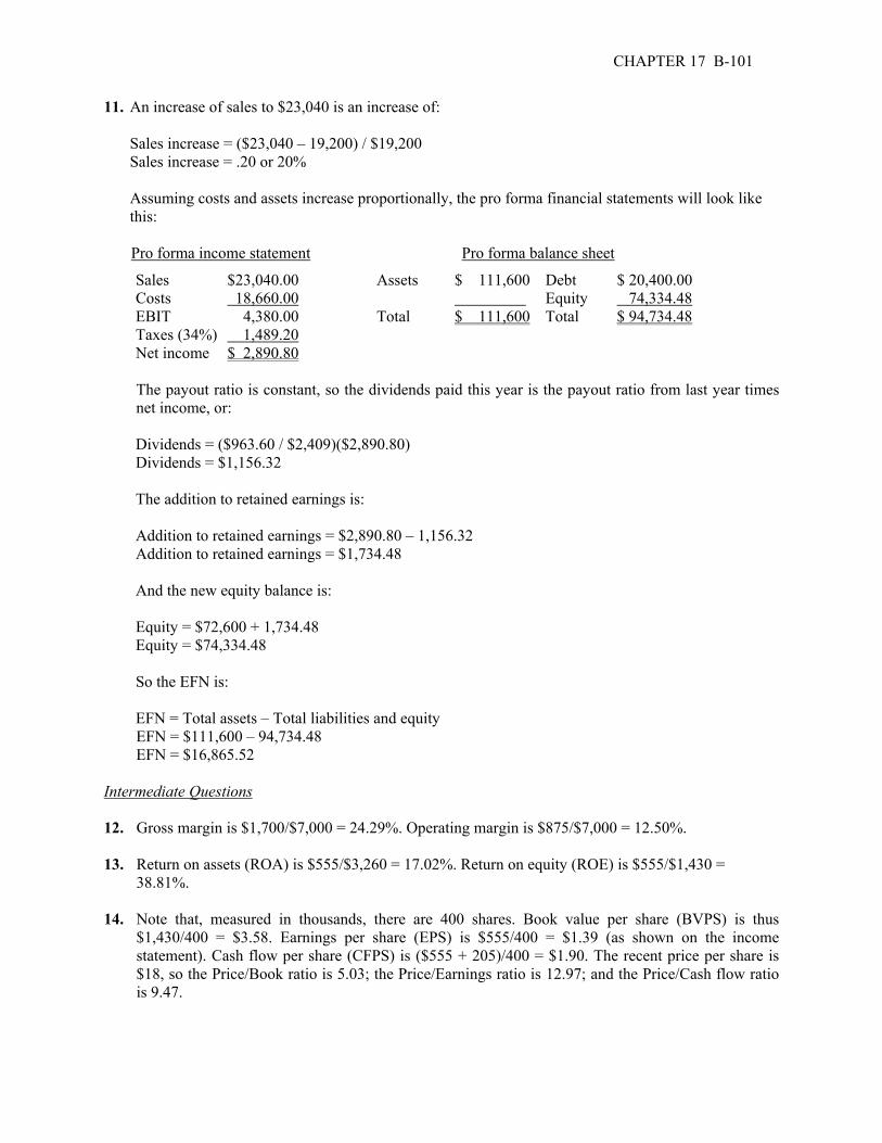
CHAPTER 17 B-101
11. An increase of sales to $23,040 is an increase of: Sales increase = ($23,040 – 19,200) / $19,200 Sales increase = .20 or 20% Assuming costs and assets increase proportionally, the pro forma financial statements will look like
this: Pro forma income statement Pro forma balance sheet
Sales $23,040.00 Assets $ 111,600 Debt $ 20,400.00 Costs 18,660.00 Equity 74,334.48 EBIT 4,380.00 Total $ 111,600 Total $ 94,734.48 Taxes (34%) 1,489.20 Net income $ 2,890.80 The payout ratio is constant, so the dividends paid this year is the payout ratio from last year times
net income, or: Dividends = ($963.60 / $2,409)($2,890.80) Dividends = $1,156.32 The addition to retained earnings is: Addition to retained earnings = $2,890.80 – 1,156.32 Addition to retained earnings = $1,734.48 And the new equity balance is: Equity = $72,600 + 1,734.48 Equity = $74,334.48 So the EFN is: EFN = Total assets – Total liabilities and equity EFN = $111,600 – 94,734.48 EFN = $16,865.52 Intermediate Questions 12. Gross margin is $1,700/$7,000 = 24.29%. Operating margin is $875/$7,000 = 12.50%. 13. Return on assets (ROA) is $555/$3,260 = 17.02%. Return on equity (ROE) is $555/$1,430 =
38.81%. 14. Note that, measured in thousands, there are 400 shares. Book value per share (BVPS) is thus
$1,430/400 = $3.58. Earnings per share (EPS) is $555/400 = $1.39 (as shown on the income statement). Cash flow per share (CFPS) is ($555 + 205)/400 = $1.90. The recent price per share is $18, so the Price/Book ratio is 5.03; the Price/Earnings ratio is 12.97; and the Price/Cash flow ratio is 9.47.
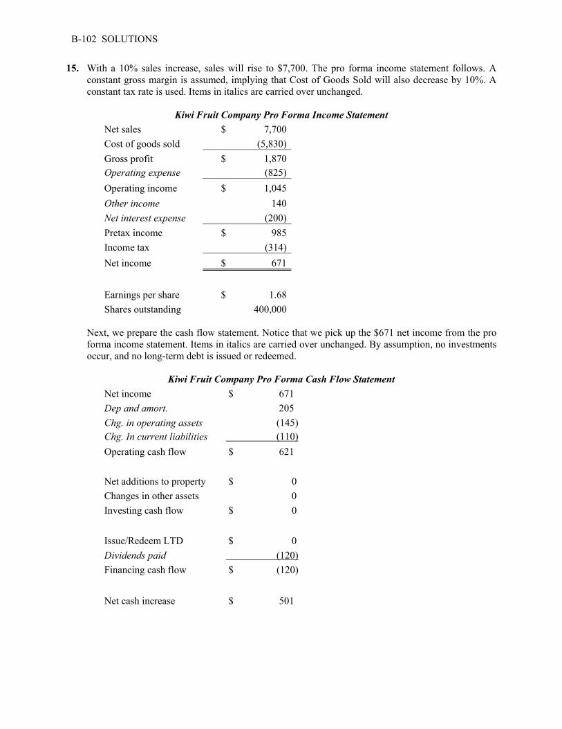
B-102 SOLUTIONS
15. With a 10% sales increase, sales will rise to $7,700. The pro forma income statement follows. A constant gross margin is assumed, implying that Cost of Goods Sold will also decrease by 10%. A constant tax rate is used. Items in italics are carried over unchanged.
Kiwi Fruit Company Pro Forma Income Statement
Net sales $ 7,700 Cost of goods sold (5,830) Gross profit $ 1,870 Operating expense (825) Operating income $ 1,045 Other income 140 Net interest expense (200) Pretax income $ 985 Income tax (314) Net income $ 671
Earnings per share $ 1.68 Shares outstanding 400,000
Next, we prepare the cash flow statement. Notice that we pick up the $671 net income from the pro
forma income statement. Items in italics are carried over unchanged. By assumption, no investments occur, and no long-term debt is issued or redeemed.
Kiwi Fruit Company Pro Forma Cash Flow Statement
Net income $ 671 Dep and amort. 205 Chg. in operating assets (145) Chg. In current liabilities (110) Operating cash flow $ 621 Net additions to property $ 0 Changes in other assets 0 Investing cash flow $ 0 Issue/Redeem LTD $ 0 Dividends paid (120) Financing cash flow $ (120) Net cash increase $ 501

CHAPTER 17 B-103
Finally, we have the balance sheet. Cash rises by the $501. Net cash flow from the cash flow statement. The $145 increase in Operating Assets and the $110 decrease in Current Liabilities are also from the cash flow statement. The $205 reduction in Property, Plant, and Equipment is the amount of the depreciation deduction shown on the cash flow statement. The increase in retained earnings is equal to pro forma Net Income less pro forma Dividends.
Kiwi Fruit Company Pro Forma Balance Sheet
Cash and equiv. $ 941 Operating assets 675 PP & E 1,995 Other assets 90 Total assets $ 3,701 Current liabilities $ 340 Long-term debt 1,260 Other liabilities 120 Total liabilities $ 1,720 Paid in capital $ 340 Retained earnings 1,981 Total equity $ 1,981 Total L&E $ 3,701
16. Using the benchmarks from question 14, projected stock prices are: BVPS × P/B = $4.95 × 5.03 = $24.93 EPS × P/E = $1.68 × 12.97 = $21.75 CFPS × P/CF = $2.19 × 9.47 = $20.74 Thus, projected prices assuming a 10% sales increase are in the $20.74 – $24.93 range. 17. Full capacity sales = $510,000 / .85 Full capacity sales = $600,000 The maximum sales growth is the full capacity sales divided by the current sales, so: Maximum sales growth = ($600,000 / $510,000) – 1 Maximum sales growth = .1765 or 17.65%

B-104 SOLUTIONS
18. To find the new level of fixed assets, we need to find the current percentage of fixed assets to full capacity sales. Doing so, we find:
Fixed assets / Full capacity sales = $415,000 / $600,000 Fixed assets / Full capacity sales = .6917 Next, we calculate the total dollar amount of fixed assets needed at the new sales figure. Total fixed assets = .6917($680,000) Total fixed assets = $470,333.33 The new fixed assets necessary is the total fixed assets at the new sales figure minus the current level
of fixed assets. New fixed assets = $470,333.33 – 415,000 New fixed assets = $55,333.33 19. Assuming costs vary with sales and a 20 percent increase in sales, the pro forma income statement
will look like this: MOOSE TOURS INC. Pro Forma Income Statement Sales $ 1,086,000 Costs 852,000 Other expenses 14,400 EBIT $ 219,600 Interest 19,700 Taxable income $ 199,900 Taxes(35%) 69,965 Net income $ 129,935 The payout ratio is constant, so the dividends paid this year is the payout ratio from last year times
net income, or: Dividends = ($42,458/$106,145)($129,935) Dividends = $51,974 And the addition to retained earnings will be: Addition to retained earnings = $129,935 – 51,974 Addition to retained earnings = $77,961 The new accumulated retained earnings on the pro forma balance sheet will be: New accumulated retained earnings = $257,000 + 77,961 New accumulated retained earnings = $334,961

CHAPTER 17 B-105
The pro forma balance sheet will look like this:
MOOSE TOURS INC. Pro Forma Balance Sheet
Assets Liabilities and Owners’ Equity
Current assets Current liabilities Cash $ 30,000 Accounts payable $ 78,000 Accounts receivable 51,600 Notes payable 9,000 Inventory 91,200 Total $ 87,000 Total $ 172,800 Long-term debt 156,000 Fixed assets Net plant and Owners’ equity equipment 436,800 Common stock and paid-in surplus $ 21,000 Retained earnings 334,961 Total $ 355,961 Total liabilities and owners’ Total assets $ 609,600 equity $ 598,961 So, the EFN is: EFN = Total assets – Total liabilities and equity EFN = $609,600 – 598,961 EFN = $10,639 20. First, we need to calculate full capacity sales, which is: Full capacity sales = $905,000 / .80 Full capacity sales = $1,131,250 The capital intensity ratio at full capacity sales is: Capital intensity ratio = Fixed assets / Full capacity sales Capital intensity ratio = $364,000 / $1,131,250 Capital intensity ratio = .32177 The fixed assets required at full capacity sales is the capital intensity ratio times the projected sales
level: Total fixed assets = .32177($1,086,000) = $349,440 So, EFN is: EFN = ($172,800 + 349,440) – $598,961 = –$76,721 Note that this solution assumes that fixed assets are decreased (sold) so the company has a 100
percent fixed asset utilization. If we assume fixed assets are not sold, the answer becomes: EFN = ($172,800 + 364,000) – $598,961 = –$62,161

Chapter 18 Corporate Bonds
Concept Questions 1. The four main types are debentures, mortgage bonds, collateral trust bonds, and equipment trust
certificates. 2. A bond refunding is a call in which an outstanding issue is replaced with a lower coupon issue. The
point is simply to replace a relatively high coupon issue with a lower coupon issue. All bond refundings involve a call, but not all calls involve a refunding. For example, an issue may be called, but not replaced.
3. Call protection refers to the period during which the bond is not callable, typically five to ten years
for a corporate bond. The call premium is the amount above par the issuer must pay to call the bond; it generally declines to zero through time.
4. A put bond gives the owner the right to force the issuer to buy the bond back, typically either at face
value or according to a preset price schedule. Obviously, the put feature is very desirable from the owner’s perspective, but not the issuer’s.
5. All else the same, a callable bond will have a higher coupon rate (because buyers don’t like call
features and, therefore, demand a higher coupon); a putable bond will have a lower coupon rate (because buyers like put features).
6. A convertible bond converts into the issuer’s stock. An exchangeable bond converts into the stock of
some other entity. Typically, with an exchangeable bond, the issuer already owns the stock into which the issue can be converted.
7. Event risk refers to a sudden decline in credit quality resulting from a significant structural or
financial change. The put feature is intended to protect holders against event risk; it works great as long as the issuer has the financial strength to fulfill its obligation to buy back the issue on demand.
8. The advantage is that the coupon adjusts up when interest rates rise, so the bond’s price won’t fall (at
least not nearly as much as it would have). It cuts both ways, however. The coupon will fall if interest rates decline, so the owner will not experience the gains that otherwise would have occurred.
9. Effective duration is a more accurate measure of interest rate risk because it measures the actual
price change for a given change in yield after accounting for any embedded options. By contrast, Macaulay and Modified duration are only approximations and do not account for the price effects of embedded options.
10. Some examples of embedded options in bonds are: 1) Put bonds have a put option feature that gives
the bondholder the right to sell the bond back to the issuer at a preset price. The put feature makes the bond more valuable to the bondholder so a put bond has a higher price than a comparable non-putable bond. 2) Convertible bonds have a call option feature that gives the bondholder the right to buy stock from the issuer at a preset price. The call option makes the bond more valuable to the bondholder so a convertible bond has a higher price than a comparable non-convertible bond. 3) Callable bonds have a call option feature that gives the issuer the right to buy the bonds back from

CHAPTER 18 B-107
the bondholder at a preset price. The call feature makes the bond less valuable to the bondholder so a callable bond has a lower price than a comparable non-callable bond.
11. The critical distinction lies in their credit ratings when they were first issued. Original issue junk
refers to a bond that had a credit rating below investment grade when it was first issued. A fallen angel had a credit rating of investment grade when it was first issued, but has since fallen to below investment grade.
12. Conceptually, they are the same thing. A put bond gives the owner the right to force the issuer to buy
the bond back, typically at face value. An extendible bond gives the owner the right to receive face value on the extension date or receive another bond. In both cases, the owner can have either face value or a bond. In practice, put bonds can be put on multiple dates (usually the coupon dates); whereas, an extendible bond may only have one extension date. Also, if an extendible bond is extended, the new bond may not have the same coupon.
13. Because of the negative convexity effect, callable bonds cannot rise in value as far as noncallable
bonds, so they do have less interest rate sensitivity. Also, a callable bond may “mature” sooner than an otherwise identical noncallable issue (because it is called), so this shorter effective maturity also means less interest rate sensitivity. Unfortunately, the smaller interest rate sensitivity is almost all on the upside, so it is not a good thing.
14. A refunding provision restricts the ability of an issuer to call their bonds. Such a provision specifies
that the issuer cannot call their bonds for the purpose of refunding their debt with a new bond issue. Since this is the most common reason that bonds are called, i.e., for a refunding. A bond issue with a refunding provision is far less likely to be called by its issuer than a comparable callable bond without a refunding provision.
15. The floating coupon in this case acts like a rocket booster, magnifying the gains and losses that occur
from changes in interest rates. Solutions to Questions and Problems NOTE: All end of chapter problems were solved using a spreadsheet. Many problems require multiple steps. Due to space and readability constraints, when these intermediate steps are included in this solutions manual, rounding may appear to have occurred. However, the final answer for each problem is found without rounding during any step in the problem. Core Questions 1. $1,000/35 = $28.57 2. $1,000/18 = $55.56 3. $1,000/$42 = 23.81 4. 45 × $26 = $1,170 5. 20 × $47 = $940 6. $896/$32 = 28.00

B-108 SOLUTIONS
7. 112% – 3 × 2% = 106% 8. P = $1,029.07 = $40(PVIFA4.325%,10) + $1000(PVF4.325%,10) + CP(PVF.325%,10); CP = $84.00 9. The minimum value is the larger of the conversion value or the intrinsic bond value. The conversion
value is 20 × $53 = $1,060. To calculate the intrinsic bond value, note that we have a face value of $1,000 (by assumption), a semiannual coupon of $45, an annual yield of 10 percent (5 percent per half-year), and 10 years to maturity (20 half-years). Using the standard bond pricing formula from our previous chapter, the bond’s price if it were not convertible is $937.69. Thus, this convertible bond will sell for at least (if not more than) $1,060.
10. You can convert or tender the bond (i.e., surrender the bond in exchange for the call price). If you
convert, you get stock worth 30 × $38 = $1,140. If you tender, you get $1,100 (110 percent of par). It’s a no-brainer: convert.
Intermediate Questions 11. Duration to maturity = (1.035/.07) – [(1.035 + 30(.10 – .07)) / (.07 + .10(1.03560 – 1))] Duration to maturity = 12.232 years Duration to call = (1.035/.07) – [(1.035 + 10(.10 – .07)) / (.07 + .10(1.03510 – 1))] = 6.885 years The duration to call is the more relevant number in this case. With interest rates lower than the
coupon rate, it is likely the company will call the bond in ten years and refinance at a lower interest rate. However, if interest rates rise to 10 percent or higher in the next ten years, the bond will likely not be called.
AIMR suggested answers: 12. Conversion value = $40 × 22 = $880; Conversion price = $1,050 / 22 = $47.73 13. An increase in the stock price volatility increases the bond price. The conversion option on the stock
becomes more valuable. An increase in interest rate volatility decreases the bond value. The chance of the bond being called increases, causing the value of the call option on the bond to become more valuable.
14. Conversion price = $980 / 25 = $39.20 One-year bond return = ($1,125 + 40 – 980) / $980 = 18.88% One-year stock return = ($45 – 35) / 35 = 28.57% 15. The two components are the straight bond value (its value as a bond) and the option value (the value
associated with the potential conversion into equity). The increase in equity price does not affect the straight value of the Ytel convertible but does
increase the call option component value significantly, because the call becomes deep in the money when the equity price is compared to the convertible’s conversion price.
The increase in interest rates decreases the straight value component (bond values decrease as
interest rates increase) of the convertible bond and increases the value of the equity call option (call option values increase as interest rates increase), though this increase may be small or unnoticeable when compared to the change in the option value resulting from the increase in the equity price.

Chapter 19 Government Bonds
Concept Questions 1. T-bills are pure discount, zero-coupon instruments with original maturities of one year or less. T-
bonds are straight coupon bonds with original maturities greater than ten years. A small number of T-bonds are callable.
2. The main difference is that T-notes have original maturities of ten years or less. Also, a small
number of T-bonds are callable, but no notes are. 3. T-bills and STRIPS. 4. Spreads are generally in the range of one to six ticks, where a tick is 1/32. The main reason that some
issues have narrower spreads is that some are much more heavily traded. In particular, the most recently auctioned issues of each maturity (called the “on-the-run” issues) dominate trading and typically have relatively narrow spreads.
5. Agencies have slightly more credit risk. They are subject to state taxes, they have a variety of call
features, and they are less liquid (and have wider spreads). These factors translate into a somewhat higher yield. Agencies offer a wider variety of maturities and bond types as well.
6. Treasuries are subject to federal taxes, but not state and local taxes. Munis are tax-exempt at the
federal level. They are usually exempt at the state level only within the issuing state. Munis can have significantly greater default risk, and they are, for the most part, much less liquid. Munis are generally callable whereas most Treasuries are not.
7. Serial bonds are bond issues that feature a series of maturity dates, meaning that the entire issue does
not come due at once. This structure reduces the chance of a “crisis at maturity” in which the issuer cannot obtain the funds needed to pay off the entire issue in one shot.
8. Variable rate notes (VRNs) are munis with floating coupons. The variable rate could increase the
possibility of default in a rising rate environment, but the inflation premium would be reduced due to the change in the rate.
9. A general obligation (GO) muni is backed by the full faith and credit (i.e., the taxing power) of the
issuer. A revenue bond is backed only by the revenue produced from a specific project or activity. 10. A private activity muni is a taxable muni. They are issued to finance activities that do not qualify for
tax-exempt status. Since they have no tax preference, they are ordinary bonds much like corporate bonds and appeal to similar investors.

B-110 SOLUTIONS
11. To a certain extent, it’s an apples and oranges issue. Munis are much less liquid, have greater default risk, are generally callable fairly early in their lives, and may be subject to state taxes if a capital gain is realized. These factors increase muni yields. As a result, when critical tax rates are calculated, they are likely to be too low. A better approach is to compare munis to corporate bonds with similar features and risks. An even better approach is to compare taxable and nontaxable munis.
12. It is true. The reason is that Treasuries are callable at par. Referring back to Chapter 10, if two
premium bonds have the same price and the same coupon rate, but different maturities (i.e., the call date and the final maturity date), the one with the shorter maturity has the lower yield. This has to be true because of the “pull to par,” i.e., the fact that for a given yield a premium bond’s price will decline as maturity approaches.
13. It is not true in general because agency securities are frequently callable at prices above par; it may
well be that the yield to call is greater for issues selling moderately above par. 14. Essentially, the tax exemption on coupon interest for the municipal bond may be more valuable than
the absence of default risk for the Treasury bond. 15. The yield spread between Treasury and municipal bonds will depend on the state of the economy
because the state of the economy largely determines the level of default risk. When the economy is doing well, municipal revenues are high and default is less likely than in a recession when municipal revenues are low.
Solutions to Questions and Problems NOTE: All end of chapter problems were solved using a spreadsheet. Many problems require multiple steps. Due to space and readability constraints, when these intermediate steps are included in this solutions manual, rounding may appear to have occurred. However, the final answer for each problem is found without rounding during any step in the problem. Core Questions 1. $10,000/(1 + .0375)40 = $2,293.38 2. $2,912 = $10,000/(1 + R)32; R = 3.93%; YTM = 3.93% × 2 = 7.86% 3. Bonds available for competitive bids = $40B – 8B = $32 billion Beginning with the highest bid ($9,410), we get $5B + 6B + 4B + 9B + 9B = $36 billion, so the
competitive bid price is $9,300. Notice the competitive bids are for a larger value than is available, so there will be an allocation. All bids above this will be accepted, along with the $8B noncompetitive bids. The amount raised is ($9,300/$10,000) × $40B = $37.20 billion.
4. $122.50(PVIFA2.80%,20) + $5,000(PVIF2.80%,20) = $4,374.76 5. $5,380 = $130(PVIFAR%,14) + $5,000(PVIFR%,14) ; R = 1.97%, YTM = 3.95% 6. $5,820 = $142.50(PVIFAR%,36) + $5,000(PVIFR%,36) ; R = 2.19%, YTM = 4.37% 7. $5,820 = $142.50(PVIFAR%,36) + $5,000(1.03)(PVIFR%,46) ; R = 1.82%, YTC = 3.64%

CHAPTER 19 B-111
8. 5.90%/(1 – .38) = 9.52% 9. 8.5%(1 – .31) = 5.87% 10. 1 – .061/.096 = 36.46% Intermediate Questions 11. You must buy at the asked yield of 4.73%. This implies a price of: $1,000 × (1 – .0473 × 160 / 360)
= $978.978 per $1,000 purchased. 12. You must sell at the bid yield of 4.76%. This implies a price of: $1,000 × (1 – .0476 × 160 / 360) =
$978.844. Thus, the dollar spread is $978.978 – 978.844 = $0.133 per $1,000 of bonds. 13. The minimum face value is $1,000. You must pay the ask price of 112:12, or 112.37500 percent of
face. This amounts to $1,123.75. 14. $32.50(PVIFA2.93%,24) + $1000(PVIF2.93%,24) = $1,054.60, which is a quoted price of 105:15 15. $1,014.6875 = $30.50(PVIFAR%,60) + $1000(PVIFR%,60) ; R = 3.00%, YTM = 5.99% 16. This is a standard yield to maturity calculation. Follow the procedure of the previous question or use
the Excel™ spreadsheet template for this problem. 17. $1,261.875 = $58.75(PVIFAR%,6) + $1000(PVIFR%,6) ; R = 1.31%, YTC = 2.62% 18. These Treasury bonds were sold in 1984 and 1985 with high coupon rates, so they are now selling
well above par and will likely be called in 2009, absent a tremendous shift in interest rates. For this reason, The Wall Street Journal reports yields to call for these bonds.
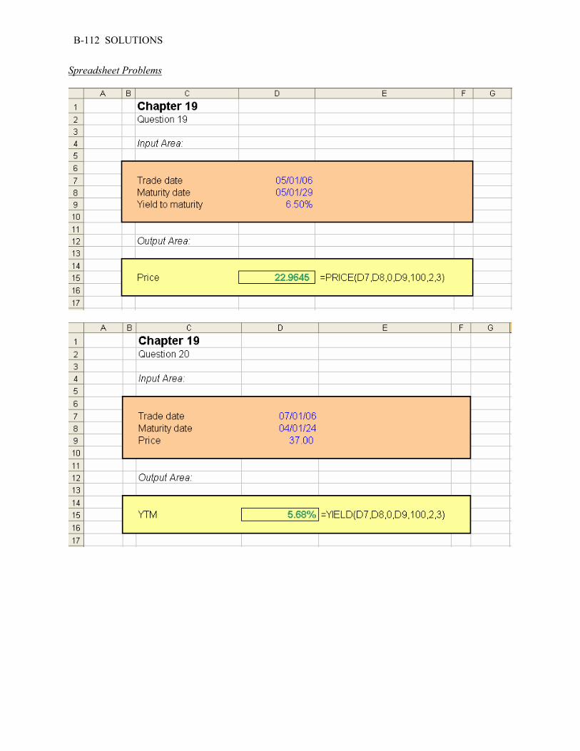
B-112 SOLUTIONS
Spreadsheet Problems

Chapter 20 Mortgage-Backed Securities
Concept Questions 1. Mortgage securitization benefits borrowers by reducing interest rates. Interest rates are reduced
because securitization increases liquidity in the mortgage market. More liquid mortgages have higher prices and, hence, lower interest rates.
2. It benefits mortgage originators by allowing them to transfer the risk associated with holding
mortgages and instead focus on what they do best, originating mortgages. Also, and equally important, by selling mortgages, originators obtain new funds to loan out.
3. For the same rate and original balance, the 15-year mortgage will have higher payments simply
because a larger principal payment must be made each month to pay off the loan over a shorter time, even though the interest component may be smaller.
4. Only GNMA is a federal agency, and GNMA securities are backed by the full faith and credit of the
U.S. government. The other two, in principle, do not have this backing. As a practical matter, however, the difference is slight.
5. It means that timely payment of both principal and interest is guaranteed. 6. Mortgages are prepaid because the underlying property is sold, interest rates fall, or the owner
otherwise wishes to refinance (perhaps to increase the loan balance as a way of obtaining funds for other purposes) or pay off the mortgage. When interest rates fall, prepayments accelerate. Larger drops lead to sharp increases in prepayment rates.
7. The call feature on a bond gives the borrower the right to buy the bond (i.e., pay off the debt) at a
fixed price. The right to prepay a mortgage gives the borrower the same right. 8. Prepayments that result purely from interest drops are a risk; the mortgage investor will have to
reinvest at a lower rate. However, some mortgages are prepaid for other reasons, such as the sale of the underlying property. This can happen even if interest rates have risen substantially; such a prepayment benefits the mortgage investors. Thus, not all prepayments are bad, just those that result in the need to reinvest at a lower rate.
9. For a fully modified mortgage pool, all cash flows are guaranteed to be paid in a timely manner,
meaning that no cash flows will be paid out late. The guarantee does, however, allow cash flows to be paid out early, which occurs in the case of defaults. When a default occurs, the remaining balance on the defaulting mortgage is paid out immediately. Thus to a mortgage pool investor, a default appears as a prepayment since in both cases an early payment of principal is realized.
B-114 SOLUTIONS
10. A collateralized mortgage obligation (CMO) is a mortgage-backed security with cash flows that are divided into multiple securities. They exist because they provide a means of altering some of the less desirable characteristics of MBS’s, thereby increasing marketability to a broader class of investors. More fundamentally, they exist because investment banks (the creators and marketers) have found them to be a profitable product! The three best-known CMO structures are interest only and principal only strips, sequential CMOs, and protected amortization class securities.
11. Every mortgage payment has an interest portion and a principal portion. IO and PO strips are very
simple CMOs; the interest and principal portions are separated into distinct payments. Holders of IO strips receive all the interest paid; the principal goes to holders of PO strips. If interest rates change, the IO strips–especially the longer dated ones–are vastly more risky. With PO strips, the only uncertainty is when the principal is paid. All PO strips-holders will receive full payment. With an IO strip, however, prepayment means that no future interest payments will be made, so the amount of interest that will be received is unknown.
12. PO strips have greater interest rate risk if we define interest rate risk to mean losses associated with
interest rate increases and gains associated with interest rate decreases. When interest rates go up, prepayments slow down, thereby postponing the time until principal is received. In this case, IO strips can actually behave like “inverse floaters.” Their value tends to rise when interest rates increase. The reason is that slowing prepayments increases the interest that will be received by IO strips-holders. However, the value of IO strips fall when interest rates decrease.
13. The A-tranche will essentially receive all of the payments, both principal and interest, until it is fully
paid off. The Z-tranche receives nothing until the A-tranche is paid off. After that, the Z-tranche receives everything. The Z-tranche is much riskier because the size and timing of the payment is more uncertain.
14. With a protected amortization class (PAC) CMO, payments are made to one group of investors
according to a set schedule. This means that the protected class investors have almost fully predictable cash flows. After protected class investors are paid, all the remaining cash flow goes to non-PAC investors, who hold PAC support or PAC companion bonds. In essence, one group of investors receives fixed payments, the other group absorbs all (or virtually all) the uncertainty created by prepayments.
15. Macaulay duration assumes fixed cash flows. With MBSs and CMOs, the payments depend on
prepayments, which in turn depend on interest rates. When prepayments pick up, duration falls, and vice versa. Thus, no single measure is accurate. Effective duration attempts to account for the possibility that mortgage pool cash flows can vary. Effective duration for a mortgage pool will typically be based on a prepayment model that accounts for the effects of changing interest rates on prepayments.

CHAPTER 20 B-115
Solutions to Questions and Problems NOTE: All end of chapter problems were solved using a spreadsheet. Many problems require multiple steps. Due to space and readability constraints, when these intermediate steps are included in this solutions manual, rounding may appear to have occurred. However, the final answer for each problem is found without rounding during any step in the problem. Core Questions 1. [$190,000(.068/12)]/{1 – [1/(1 + .068/12)360]} = $1,238.66 2. $1,060{1 – [1/(1 + .072/12)360]}/(.072/12) = $156,160.64 3. [$230,000(.069/12)]/{1 – [1/(1 + .069/12)360]} = $1,514.78 4. $1,250{1 – [1/(1 + .071/12)360]}/(.071/12) = $186,003.06 5. 1 – (1 – .04)1/12 = 0.3396% 6. 0.00583 = 1 – (1 – CPR)1/12; CPR = 6.7760% 7. $96,483 – 37,155 = $59,328 8. Payment = [$220,000(.073/12)]/{1 – [1/(1 + .073/12)360]} = $1,508.26 The interest in the first month is equal to the original loan amount ($220,000) multiplied by the
interest rate, .073/12 = .006083 per month. Thus, the interest amounts to $1,338.33. The remaining $1,508.26 – 1,338.83 = $169.92 is principal. The interest allocation for the second payment is $1,337.30, and the principal reduction is $170.96.
9. Payment = [$225,000(.081/12)]/{1 – [1/(1 + .081/12)300]} = $1,751.52 Balance = $1,751.52{1 – [1/(1 + .081/12)216]}/(.081/12) = $198,805.34 10. Payment = [$300,000(.074/12)]/{1 – [1/(1 + .074/12)360]} = $2,077.14 Balance = $2,077.14{1 – [1/(1 + .074/12)288]}/(.074/12) = $279,490.91 Intermediate Questions 11. Original payment = [$190,000(.08/12)]/{1 – [1/(1 + .08/12)360]} = $1,394.15 Balance = $1,394.15{1 – [1/(1 + .08/12)252]}/(.08/12) = $169,929.93 New payment = [$169,929.93(.06/12)]/{1 – [1/(1 + .06/12)252]} = $1,187.57 Savings = $1,194.15 – 1,187.57 = $206.59 12. Original payment = [$180,000(.085/12)]/{1 – [1/(1 + .085/12)300]} = $1,449.41 Balance = $1,449.41{1 – [1/(1 + .085/12)204]}/(.085/12) = $156,137.14 New payment = [$156,137.14(.07/12)]/{1 – [1/(1 + .07/12)204]} = $1,311.02 Savings = $1,449.41 – 1,311.02 = $138.39

B-116 SOLUTIONS
13. Original payment = [$215,000(.0685/12)]/{1 – [1/(1 + .0685/12)360]} = $1,408.81 Balance = $1,408.81{1 – [1/(1 + .0685/12)300]}/(.0685/12) = $202,055.10 New payment = [($202,055.10 + 2,500)(.0624/12)]/{1 – [1/(1 + .0624/12)300]} = $1,348.12 Savings = $1,408.81 – 1,348.12 = $60.68 14. Original payment = [$195,000(.0782/12)]/{1 – [1/(1 + .0782/12)360]} = $1,406.45 Balance = $1,406.45{1 – [1/(1 + .0782/12)288]}/(.0782/12) = $182,583.44 $182,583.44 + 3,500 = $1,406.45(PVIFAR%,288); R = 0.6330%; APR = 7.60% 15. Original payment = [$170,000(.0815/12)]/{1 – [1/(1 + .0815/12)360]} = $1,265.22 Balance = $1,265.22{1 – [1/(1 + .0815/12)96]}/(.0815/12) = $89,018.40 $89,018.40 + 3,000 = $1,265.22(PVIFAR%,96); R = 0.60270%; APR = 7.23% 16. For a seasoned 100 PSA mortgage, the CPR is 5 percent per year. PSA 50: CPR = (50/100)(.05) = 2.50% PSA 200: CPR = (200/100)(.05) = 10.00% PSA 400: CPR = (400/100)(.05) = 20.00% These CPRs have two, more or less equivalent interpretations. They are an estimate of the
probability that any given mortgage in the pool will prepay in a given year. A more useful interpretation is that they are an estimate of the percentage of outstanding principal that will be prepaid in a given year. In other words, if the odds of prepayment are 5 percent for any given mortgage, then we expect that 5 percent of all mortgages will prepay, meaning that 5 percent of the principal in a mortgage pool will be prepaid per year.
17. PSA 50: SMM = 1 – (1 – .0250)1/12 = 0.2108% PSA 200: SMM = 1 – (1 – .10)1/12 = 0.8742% PSA 400: SMM = 1 – (1 – .20)1/12 = 1.8423% Notice that the 400 PSA is not simply double the 200; there’s a compound interest-type effect in the
calculation. The SMM estimates the probability of prepayment in a given month. Thus, with 50 PSA, it is estimated that .2108 percent of mortgages will prepay in a given month.
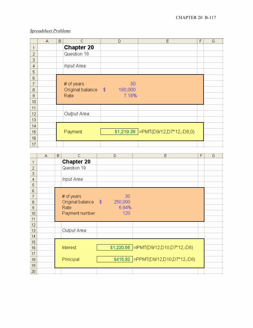
CHAPTER 20 B-117
Spreadsheet Problems
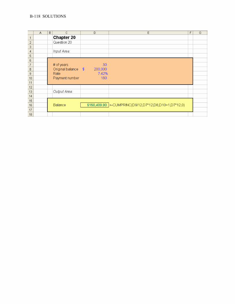
B-118 SOLUTIONS


