1

Joint Communication and Control for WirelessAutonomous Vehicular Platoon Systems

Tengchan Zeng1, Omid Semiari2, Walid Saad1, and Mehdi Bennis31 Wireless@VT, Department of Electrical and Computer Engineering, Virginia Tech, Blacksburg, VA, USA,

Emails:tengchan,walids@vt.edu.2 Department of Electrical and Computer Engineering, University of Colorado Colorado Springs, Colorado

Springs, CO, USA,

Email: osemiari@uccs.edu.3 Centre for Wireless Communications, University of Oulu, Oulu, Finland, Email: mehdi.bennis@oulu.fi.

AbstractAutonomous vehicular platoons will play an important role in improving on-road safety in tomor-

row’s smart cities. Vehicles in an autonomous platoon can exploit vehicle-to-vehicle (V2V) communica-

tions to collect environmental information so as to maintain the target velocity and inter-vehicle distance.

However, due to the uncertainty of the wireless channel, V2V communications within a platoon will

experience a wireless system delay. Such system delay can impair the vehicles’ ability to stabilize their

velocity and distances within their platoon. In this paper, the problem of integrated communication and

control system is studied for wireless connected autonomous vehicular platoons. In particular, a novel

framework is proposed for optimizing a platoon’s operation while jointly taking into account the delay

of the wireless V2V network and the stability of the vehicle’s control system. First, stability analysis

for the control system is performed and the maximum wireless system delay requirements which can

prevent the instability of the control system are derived. Then, delay analysis is conducted to determine

the end-to-end delay, including queuing, processing, and transmission delay for the V2V link in the

wireless network. Subsequently, using the derived wireless delay, a lower bound and an approximated

expression of the reliability for the wireless system, defined as the probability that the wireless system

meets the control system’s delay needs, are derived. Then, the parameters of the control system are

optimized in a way to maximize the derived wireless system reliability. Simulation results corroborate

the analytical derivations and study the impact of parameters, such as the packet size and the platoon

size, on the reliability performance of the vehicular platoon. More importantly, the simulation results

shed light on the benefits of integrating control system and wireless network design while providing

guidelines for designing an autonomous platoon so as to realize the required wireless network reliability

and control system stability.

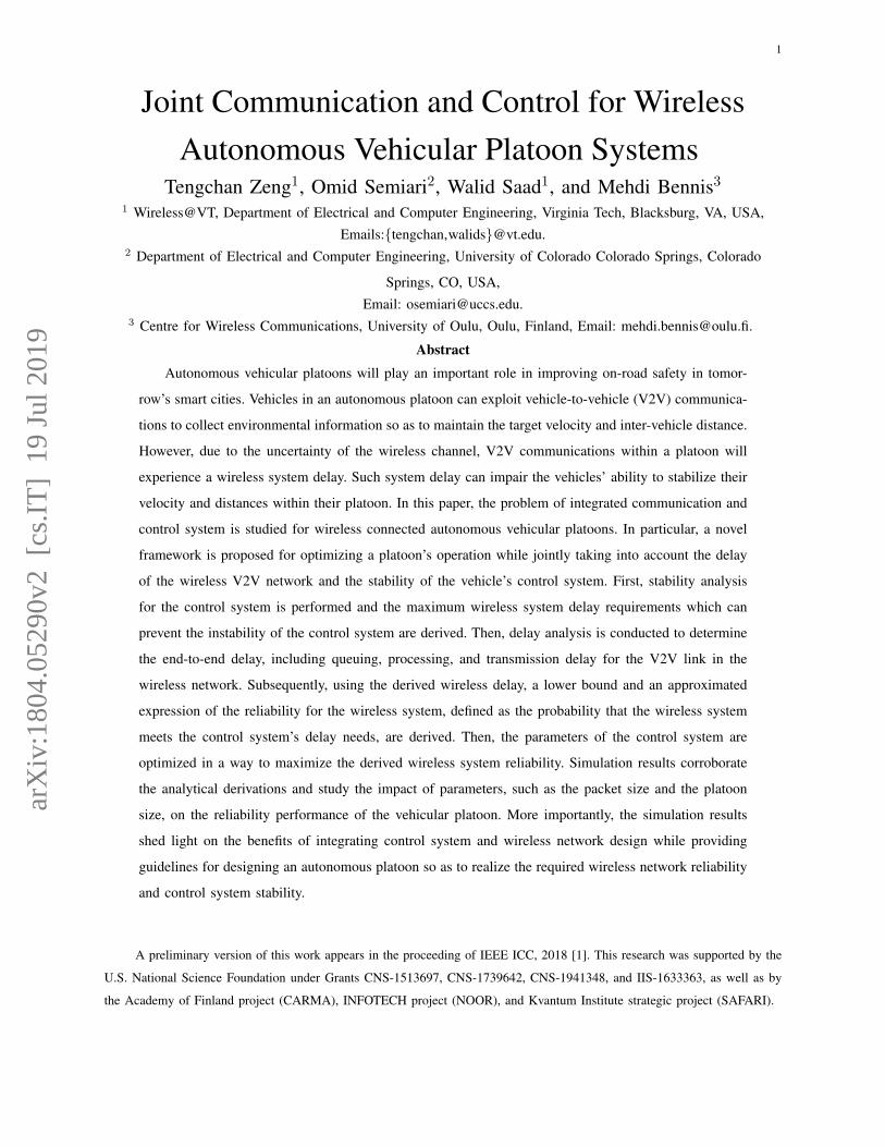
A preliminary version of this work appears in the proceeding of IEEE ICC, 2018 [1]. This research was supported by the

U.S. National Science Foundation under Grants CNS-1513697, CNS-1739642, CNS-1941348, and IIS-1633363, as well as by

the Academy of Finland project (CARMA), INFOTECH project (NOOR), and Kvantum Institute strategic project (SAFARI).

arX

iv:1

804.

0529

0v2

[cs

.IT

] 1

9 Ju

l 201

9

2

I. INTRODUCTION

Intelligent transportation systems (ITSs) will be a major component of tomorrow’s smart

cities. In essence, ITSs will provide a much safer and more coordinated traffic network by

using efficient traffic management approaches [2]. One promising ITS service is the so-called

autonomous vehicular platoon system, which is essentially a group of vehicles that operate

together and continuously coordinate their speed and distance. By allowing autonomous vehicles

to self-organize into a platoon, the road capacity can increase so as to prevent traffic jams [3].

Also, vehicles in the platoon can raise the fuel efficiency [4]. Furthermore, platoons can provide

passengers with more comfortable trips, especially during long travels [5].

To reap the benefits of platooning, one must ensure that each vehicle in the platoon has

enough awareness of its relative distance and velocity with its surrounding vehicles. This is

needed to enable vehicles in a platoon to coordinate their acceleration and deceleration. In

particular, enabling autonomous platooning requires two technologies: vehicle-to-vehicle (V2V)

communications [6] and cooperative adaptive cruise control (CACC) [7]. V2V communications

enable vehicles to exchange information, such as high definition (HD) maps, velocity, and

acceleration [8]. Meanwhile, CACC is primarily a control system that allows control of the

distances between vehicles using information collected by sensors and V2V links. Effectively

integrating the operation of the CACC system and the V2V communication network is central

for successful platooning in ITSs.

Nevertheless, due to the uncertainty of the wireless channel, V2V communication links will

inevitably suffer from time-varying delays, which can be as high as hundreds of millisecond

[9]. Unfortunately, if the delayed information is used in the design of the autonomous vehicles’

control system, such information can jeopardize the stable operation of the platoon [10]. There-

fore, to maintain the stability of a platoon, the control system must be robust to such wireless

transmission delays. To this end, one must jointly consider the control and wireless systems of

a platoon to guarantee low latency and stability.

The prior art on vehicular platooning can be grouped into two categories. The first category

focuses on the performance analysis, such as interference management [11]–[14], security system

design [15], and transmission delay analysis [16]–[18], for the inter-vehicle communication

network. The second category designs control strategies that guarantee the stability of the platoon

system. Such strategies include adaptive cruise control (ACC) [19], enhanced ACC [20], and

connected cruise control (CCC) [21]. However, these works are limited in two aspects. The

3

communication-centric works in [11]–[18] completely abstract the control system and do not

study the impact of wireless communications on the platoon’s stability. Meanwhile, the control-

centric works in [19]–[21] focus solely on the stability, while assuming a deterministic perfor-

mance from the communication network. Such an assumption is not practical for platoons that

coexist with 5G cellular networks, since interference from uncoordinated cochannel transmissions

by other users, vehicles, and platoons can substantially impact the system’s performance. Clearly,

despite the interdependent performance of communication and control systems in a platoon, there

is a lack in existing works that jointly study the wireless and control system performance for

vehicular platoons.

The main contribution of this paper is a novel, integrated control system and V2V wireless

communication network framework for autonomous vehicular platoons. In particular, we first

analyze the stability of the control system in a platoon, and, then, we determine the maximum

tolerable transmission delay to maintain the stability of the platoon. Next, we use stochastic

geometry and queuing theory to perform end-to-end delay analysis for the V2V communication

link between two consecutive vehicles in the platoon. Based on the maximum wireless system

delay and the theoretical end-to-end delay, we conduct reliability analysis for the wireless

communication network. Here, reliability is defined as the possibility of the wireless system

meeting the maximum delay requirements from the control system. Finally, we optimize the

design of the control system to improve the reliability of the communication network. To our

best knowledge, this is the first work that considers both control system and V2V wireless

communication network for a wireless connected autonomous platoon. The novelty of this work

lies in the following key contributions:

• We propose an integrated control system and V2V wireless communication performance

analysis framework to guarantee the overall operation of wireless connected vehicular

platoons. In particular, we analyze two types of control system stability, plant stability

and string stability, for the platoon, and derive the maximum wireless system delay that

guarantees both types of stability. We then consider a highway model that models the

distribution of platoon vehicles and non-platoon vehicles and derive the complementary

cumulative density function (CCDF) for the signal-to-interference-plus-noise-ratio (SINR)

of V2V communication links. Given the derived CCDF expression, we make use of queuing

theory to determine the end-to-end wireless system delay, including queuing, processing,

and transmission delay for the V2V link in the platoon.

4

• We use the derived delay to study how the wireless network can meet the control system’s

delay needs. In particular, we derive a lower bound on the wireless network reliability

(in terms of delay) needed to guarantee plant and string stability. In addition, we find an

approximated reliability expression for vehicular network scenarios in which the wireless

system delay is dominated by the transmission delay.

• We propose two optimization mechanisms to effectively design the control system so as to

improve the reliability of the wireless network. In particular, we use the dual update method

to find the sub-optimal control system parameters that increase the lower bound and the

approximated values of the wireless network reliability.

• Simulation results corroborate the stability and SINR analysis and validate the effectiveness

of the proposed joint control and communication framework. The results show how key

parameters, such as the distribution density of non-platoon vehicles, packet size, spacing

between two platoon vehicles, and platoon size, affect the reliability of a platoon. The

results also show that, by optimizing the control system, the approximated reliability and

the reliability lower bound of the wireless network can increase by as much as 15% and

15%, respectively.

Combining the theoretical analysis and simulation results, we obtain important guidelines for

the joint design of the wireless network and the control system in vehicular platoons. In particular,

system parameters, such as the number of followers, the bandwidth, and the spacing between

two consecutive vehicles in the platoon should be properly selected to ensure the stability of

the control system. Meanwhile, the control system should also be optimized to relax the delay

constraints of the wireless network, thereby improving the reliability of the platoon system.

The rest of the paper is organized as follows. Section II presents the system model. In Section

III, we perform stability analysis for the autonomous platoon. The end-to-end delay and reliability

analysis are presented in Section IV. Section V shows how to optimize the design of the control

system. Section VI provides the simulation results, and conclusions are drawn in Section VII.

II. SYSTEM MODEL

In this section, we first discuss the highway traffic model for the platoon, the channel model

for the vehicular communication network, and the vehicles’ control model. We will then perform

an interference analysis for vehicles within the platoon and introduce the joint communication

and control problem for wireless autonomous vehicular platoons.

5

l

Platoon vehicle Transmitting non-platoon vehicle Receiving non-platoon vehicle

V2V link

BS/ Road side unit

Cellular link

x

y

4

1

2

n=3

N=5

BS/ Road side unit

Φ1

Φ2

Φ4

Φ5

Ψ1 Ψ2

Fig. 1. A highway traffic model where vehicles in the dashed ellipse operate in a platoon and other vehicles out of

the platoon drive individually.

A. Highway Traffic Model

Consider a highway traffic model that is composed of a number of autonomous vehicles

driving in a platoon and multiple vehicles driving individually, as shown in Fig. 1. All vehicles

(inside and outside the platoon) communicate with one another using V2V communications.

Vehicles can also exchange information with nearby road side units or cellular base stations (BSs)

via vehicle-to-infrastructure (V2I) communications. Although both the IEEE 802.11p standard

and cellular vehicle-to-everything (C-V2X) communications are widely considered for vehicular

networking, here, we focus on the C-V2X communication due to its enhanced performance

(e.g., extended communication range and achieve a higher reliability) compared with the IEEE

802.11p standard [22]. Each lane in the highway model has the same width l, and vehicles are

considered to travel along the horizontal axes in these lanes. As shown in Fig. 1, we label all

N lanes based on their relative locations and we assume that platoon vehicles are moving in

platoon lane n while the other N − 1 lanes are designated as non-platoon lanes. Accordingly,

we define the set Φ of transmitting vehicles driving on non-platoon lanes and the set Ψ of

transmitting non-platoon vehicles on the platoon lane. In particular, Φ consists of multiple subsets

Φh, h ∈ 1, 2, ..., n−1, n+1, ..., N, of transmitting non-platoon vehicles on non-platoon lane h.

However, set Ψ is only composed of two subsets of transmitting vehicles: subset Ψ1 of vehicles

that drive ahead of the platoon and subset Ψ2 that includes vehicles moving behind the platoon.

When considering a highway model in a large area, we can leverage spatial point processes

from stochastic geometry to capture the distribution of transmitting non-platoon vehicles in

the highway [23]. In particular, we characterize the distribution of transmitting vehicles on

non-platoon lane h 6= n, as a homogeneous Poisson point process (PPP) with density λh.

6

. . .

. . .

V2V link

vM v2 v1 v0

xM x1 x0δ2 δ1

LeaderFollowers

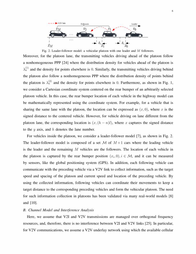
Fig. 2. Leader-follower model: a vehicular platoon with one leader and M followers.

Moreover, for the platoon lane, the transmitting vehicles driving ahead of the platoon follow

a nonhomogeneous PPP [24] where the distribution density for vehicles ahead of the platoon is

λ(1)n and the density for points elsewhere is 0. Similarly, the transmitting vehicles driving behind

the platoon also follow a nonhomogeneous PPP where the distribution density of points behind

the platoon is λ(2)n and the density for points elsewhere is 0. Furthermore, as shown in Fig. 1,

we consider a Cartesian coordinate system centered on the rear bumper of an arbitrarily selected

platoon vehicle. In this case, the rear bumper location of each vehicle in the highway model can

be mathematically represented using the coordinate system. For example, for a vehicle that is

sharing the same lane with the platoon, the location can be expressed as (x, 0), where x is the

signed distance to the centered vehicle. However, for vehicle driving on lane different from the

platoon lane, the corresponding location is (x, (h − n)l), where x captures the signed distance

to the y axis, and h denotes the lane number.

For vehicles inside the platoon, we consider a leader-follower model [7], as shown in Fig. 2.

The leader-follower model is composed of a set M of M+1 cars where the leading vehicle

is the leader and the remaining M vehicles are the followers. The location of each vehicle in

the platoon is captured by the rear bumper position (xi, 0), i ∈ M, and it can be measured

by sensors, like the global positioning system (GPS). In addition, each following vehicle can

communicate with the preceding vehicle via a V2V link to collect information, such as the target

speed and spacing of the platoon and current speed and location of the preceding vehicle. By

using the collected information, following vehicles can coordinate their movements to keep a

target distance to the corresponding preceding vehicles and form the vehicular platoon. The need

for such information collection in platoons has been validated via many real-world models [8]

and [10].

B. Channel Model and Interference Analysis

Here, we assume that V2I and V2V transmissions are managed over orthogonal frequency

resources, and, therefore, there is no interference between V2I and V2V links [25]. In particular,

for V2V communications, we assume a V2V underlay network using which the available cellular

7

bandwidth ω is reused by all V2V links outside the platoon. Meanwhile, we consider an

orthogonal frequency-division multiple access (OFDMA) scheme in which the BS will allocate

orthogonal subcarriers to platoon vehicles so as to avoid interference between concurrent V2V

transmissions inside the platoon1. Such an allocation is possible given that the typical platoon

will not have a very large number of vehicles and, hence, will require only a few subcarriers.

However, due to bandwidth sharing with non-platoon vehicles, the followers will encounter

interference from other V2V links outside the platoon. According to the channel measurement

results presented in [27] and [28], we model the V2V channels in the platoon as independent

Nakagami channels with parameter m to characterize a wide range of fading environments

for V2V links. Also, in general, Nakagami channel models can describe a wide range of

fading environment of vehicular networks [28]. Therefore, in the platoon, the received power

at any follower i ∈ M from the transmission of platoon car i−1 by using subcarrier j is

Pi,j(t)=Ptgi,j(t)(di−1,i(t))−α, where Pt is the transmit power of each vehicle, gi,j(t) follows a

Gamma distribution with shape parameter m, di−1,i(t) is the distance between vehicles i−1 and

i inside the platoon, and α is the path loss exponent. Since line-of-sight signals from non-platoon

vehicles to the platoon vehicles do not always exist, we model these channels as independent

Rayleigh fading channels [29]. Consequently, the overall interference at car i is the sum of two

following interference terms:

Inon-platooni (t) =

n−1∑j1=1

∑c∈Φj1

Ptgc,i(t)(dc,i(t))−α +

N∑j2=n+1

∑c∈Φj2

Ptgc,i(t)(dc,i(t))−α, (1)

Iplatooni (t) =

2∑j3=1

∑c∈Ψj3

Ptgc,i(t)(dc,i(t))−α, (2)

where j1 ∈ [1, ..., n − 1], j2 ∈ [n + 1, ..., N ], j3 ∈ [1, 2], dc,i(t) denotes the distance between

vehicles c and i, and gc,i(t) refers to the channel gain from vehicle c to i at time t, which

follows an exponential distribution. Using (1) and (2), the SINR of the V2V link on subcarrier

j from car i− 1 to i will be:

γi,j(t) =Pi,j(t)

Inon-platooni (t) + Iplatoon

i (t) + σ2, (3)

1Due to the small velocity difference between platoon vehicles and the use of sub-6 GHz frequencies, effect of the Doppler

shift can be neglected (or assumed to be handled via proper Doppler shift mitigation techniques) [26].

8

where σ2 is the variance of Gaussian noise. Using (3), we can obtain the throughput of the V2V

link between vehicles i− 1 and i as Ri,j(t) = ωj log2(1 + γi,j(t)), where ωj is the bandwidth of

subcarrier j. Here, we assume that the bandwidth for each subcarrier is ωM

.

C. Control Model

To realize the target spacing for the platoon, the CACC system in each vehicle will brake or

accelerate according to the difference between the actual distance and target spacing slot to the

preceding vehicle. That is, if the difference is positive, the vehicle must speed up so that the

distance to the preceding car meets the platoon’s target spacing. Otherwise, the vehicle must

slow down. This distance difference is defined as the spacing error δi(t):

δi(t) = xi−1(t)− xi(t)− L(t), i ∈M, (4)

where L(t) is the target spacing at time t for the platoon. The distance difference, di−1,i(t) =

xi−1(t)−xi(t), is also commonly known as the headway. In addition, the velocity error will be:

zi(t) = vi(t)− v(t), (5)

where vi(t) represents the velocity of vehicle i at time t, and v(t) is the target velocity at time

t for the platoon. Similar to [7], we assume that the spacing requirement L(t) and velocity

requirement v(t) are constants at time t. Also, similar to the optimal velocity model (OVM)

introduced in [30], to realize the stability of a platoon system, the acceleration or deceleration

of each vehicle must be determined by two components: 1) the difference between headway-

dependent and actual velocities, and 2) the velocity difference between a given vehicle and its

preceding vehicle. Hence, to guarantee that both velocity and spacing errors converge to zero,

we use the following control law to determine the acceleration ui(t) of vehicle i [30]

ui(t) = ai[V (di−1,i(t− τi−1,i(t)))− vi(t)] + bi[vi−1(t− τi−1,i(t))− vi(t)], (6)

where τi−1,i(t) captures the wireless system delay between vehicle i and its preceding vehicle,

ai is the associated gain of vehicle i for the difference of the headway-dependent velocity and

the actual speed, and bi is the associated gain of vehicle i for the velocity difference between

cars i− 1 and i. Here, we assume that, for each V2V link, the transmitter will also transmit a

timestamp when the information is sent. Thus, the receiving vehicle can measure the transmission

delay τi−1,i(t) and calculate di−1,i(t − τi−1,i(t)). Also, note that the associated gains ai and bi

essentially capture the sensibility of the CACC system to respond to changes of the distance and

9

velocity. Moreover, the headway-dependent velocity V (d) should satisfy following properties:

1) in dense traffic, the vehicle will stop, i.e., V (d) = 0 for d ≤ ddense, 2) in sparse traffic, the

vehicle can travel with its maximum speed V (d) = vmax, which is also called free-flow speed,

for d ≥ dsparse, and 3) when ddense < d < dsparse, V (d) is a monotonically increasing function of

d. We define the function V (d) [7]:

V (d) =

0, if d < ddense,

vmax ×(

d−ddensedsparse−ddense

), if ddense ≤ d ≤ dsparse,

vmax, if dsparse < d.

(7)

To guarantee the stable operation of the platoon system, it is important to jointly consider the

communication and control systems for the platoon. In particular, on the one hand, for a given

control system setup, one can design the wireless network so as to meet the delay requirement

of V2V links and prevent the instability of the control system. On the other hand, given the

state of the wireless system, one can also optimize the design of the control system to relax the

delay requirements for the communication system. In the following sections, we will first conduct

stability analysis for the control system and find the wireless system delay requirements to realize

the stable operation of the control system. Then, based on the distribution of vehicles, we derive

the CCDF of the SINR of V2V links in the platoon. To model the delay, we consider two

queues in tandem for the V2V link, and leverage queuing theory to derive the end-to-end delay,

including queuing, processing, and transmission delay. Then, we derive the lower bound and

approximated expressions for the wireless system reliability, defined as the probability that the

wireless system meets the delay requirements from the control system. Moreover, we optimize

the design for the control system to maximize the derived reliability metrics of the wireless

network.

III. STABILITY ANALYSIS OF THE CONTROL SYSTEM

For the leader-follower platoon model, the inevitable wireless system delay in (6) can neg-

atively impact the stability of the platoon system. Here, we perform stability analysis for the

control system in presence of a wireless system delay. We analyze two types of stability: plant

stability and string stability [7]. Plant stability focuses on the convergence of error terms related

to the inter-vehicle distance and velocity, while string stability pertains to the error propagation

across the platoon. Using this stability analysis, we obtain the wireless system delay thresholds

that can ensure plant and string stability for the control system.

10

A. Plant Stability

Plant stability requires all followers in a platoon to drive with the same speed as the leader

and maintain a target distance from the preceding vehicle. In other words, plant stability requires

both the spacing and speed errors of each vehicle to converge to zero. This convergence also

requires the first-order derivative of the error terms in (4) and (5) to approach to zero. Thus, we

can take the first-order derivative of (4) and (5) as:δi(t) = zi−1(t)− zi(t),

zi(t) = Aiδi(t− τi−1,i(t)) +Bizi−1(t− τi−1,i(t))− Cizi(t),(8)

where δi(t) and zi(t) are variables differentiated with respect to time t, Ai = aivmaxdsparse−ddense

, Bi = bi,

and Ci = ai + bi. Note that since the leading vehicle with index 0 always drives with the target

velocity, its velocity (spacing) error is z0(t) = 0 (δ0(t)=0). As observed from (8), to guarantee

the convergence of the derivatives, both zi(t) and δi(t) should asymptotically approach to zero.

Therefore, the zero convergence of spacing and speed errors is equivalent to the asymptotical

zero convergence of their first-order derivatives.

Then, after the BS collects spacing and velocity errors for all of the followers, we can find

the augmented error state vector e(t)=[δ1(t), δ2(t), ..., δM(t), z1(t), z2(t), ..., zM(t)]T and obtain

e(t) =

0M×M Ω1

0M×M Ω2

e(t) +M∑i=1

0M×M 0M×M

Ωi3 Ωi

4

e(t− τi−1,i(t)), (9)

where

Ω1 =

−1 0 0 . . . 0 0

1 −1 0 . . . 0 0

0 1 −1 . . . 0 0...

...... . . . ...

...

0 0 0 . . . 1 −1

M×M

, (10)

Ω2 = diag−C1,−C2...,−CMM×M , (11)

and the elements in Ωi3 ∈ RM×M and Ωi

4 ∈ RM×M are defined as

[Ωi3]m1,m2 =

Ai, if m1 = m2 = i,

0, otherwise,[Ωi

4]m1,m2 =

Bi, if m1 = i,m2 = i− 1, i > 1,

0, otherwise.(12)

11

For ease of presentation, we rewrite M 1=

0M×M Ω1

0M×M Ω2

, M i2=

0M×M 0M×M

Ωi3 Ωi

4

, and use e to

denote e(t) hereinafter. Since plant stability requires the spacing and velocity errors to converge

to zero, the error vector e = 02M×1 should be asymptotically stable.

To guarantee the plant stability for a platoon, the delay experienced by a V2V link should be

below a threshold. Next, we derive the delay threshold to guarantee plant stability.

Theorem 1. The plant stability of the platoon can be guaranteed if a2i + b2

i + 2aibi − 4ai ≥ 0

and the maximum delay of the V2V link between vehicles i − 1 and i, i ∈ M, in the platoon

satisfies:

τi−1,i(t) ≤ τ1 =λmin(M 3)

λmax

(M 4

) , (13)

whereM 3 =−2(M 1+∑M

i=1Mi2),M 4 =

∑Mi=1(M i

2M 1MT1 (M i

2)T )+∑M

i=2(M i2M

i−12 (M i−1

2 )T

(M i2)T ) + 2MkI2M×2M with k > 1, and λmax(·) and λmin(·) represent the maximum and

minimum eigenvalues of the corresponding matrix.

Proof: Please refer to Appendix A.

Hence, when a2i + b2

i + 2aibi − 4ai ≥ 0 and τi−1,i(t)≤ τ1, i∈M, the following vehicles will

eventually drive with the same speed as the leading vehicle and keep an identical distance to

the corresponding preceding vehicles.

B. String Stability

Beyond plant stability, we must ensure that the platoon is string stable. In particular, if the

disturbances, in terms of velocity or distance, of preceding vehicles do not amplify along with

the platoon, the system can have string stability and the safety of the system can be secured [3].

To find the delay requirement guaranteeing string stability, we first obtain the transfer function

between two adjacent vehicles by finding the Laplace transform of both equations in (8):

Ti(s) =zi(s)

zi−1(s)=Ai + sBie

−sτi−1,i(t)

s2 + Cis+ Ai, i ∈M. (14)

Here, without loss of generality, we assume that vehicles in the platoon are identical, and, thus,

the associated gains are equal, i.e., ai = a and bi = b, i ∈M. Based on [31], we know that string

stability is guaranteed as long as the magnitude of the transfer function satisfies |Ti(jf)| ≤ 1

for f ∈ R+, where f represents the frequency of sinusoidal excitation signals generated by

the leader. Thus, by using Pade approximation [32] for e−sτi−1,i(t) in the numerator of (14), we

12

Sensing Unit

Sensors

ADC

Processing Unit

Processor

Memory

I/OTransceiver

(a) Transmitter architecture.

Q1 Q2

Vehicle

Processor

Sensor

DataTransceiver

(b) Queuing model.

Fig. 3. Data path inside a transmitting vehicle.

can find an approximated analytical result of the maximum wireless system delay to satisfy

|Ti(jf)| ≤ 1, f ∈ R+, in the following proposition.

Proposition 1. The string stability of the system in (6) can be guaranteed if a + 2b − 2 ≥ 0,

and the maximum delay of the V2V link between vehicles i − 1 and i, i ∈ M, in the platoon

satisfies:

τi−1,i(t) ≤ τ2 =C2 − 2A−B2

2AC, (15)

where A= avmaxdsparse−ddense

, B=b, C=a+b, and τ2 is the approximated communication delay threshold.

Proof: Please refer to Appendix B.

To sum up, if a+ 2b− 2 ≥ 0 and τi−1,i(t) ≤ τ2, i ∈ M, the spacing error and velocity error

will not amplify along the string of vehicles, guaranteeing the platoon’s safety. To guarantee

both plant and string stability for a platoon, we must ensure that the delay encountered by the

V2V link is such that τi−1,i(t) ≤ min(τ1, τ2), i ∈ M, and the control gains should satisfy

a+ 2b− 2 ≥ 0 and a2 + b2 + 2ab− 4a ≥ 0.

IV. END-TO-END LATENCY ANALYSIS OF THE WIRELESS NETWORK

From the results presented in Section III, to realize the stability for the control system, the

wireless V2V network must guarantee that the maximum delay between two consecutive vehicles

in the platoon is less than a threshold. To quantify such wireless system delay, we need to know

how a data packet propagates among vehicles as well as the key factors that affect the delay

inside the platoon. As shown in Fig. 3(a), vehicular network information, such as location,

will be first collected by sensing units in the vehicle. Here, sensing units consist of analog-to-

digital converters (ADCs), which convert analog data from the sensor to digital data that can be

13

processed by the processor. Then, the processor will not only provide an interface to the sensing

unit and the transceiver and execute instructions pertaining to sensing and communication but it

is also used to calculate the current speed based on the collected GPS data. Next, the processor

will perform digital to analog conversion and then transmit the analog data to the transceiver so

as to transmit to other vehicles via V2V links. Finally, the receiving vehicles will use the recently

received information and sensor data to adjust their acceleration or deceleration based on (6).

Such information exchange is needed since vehicles must be aware of the nearby environment

so as to form a target platoon especially under extreme road situations where the velocity and

spacing requirements for the platoon can suddenly change and must be exchanged continuously

among vehicles in the platoon [8], [10], [11]. To capture the V2V communication delay in the

information exchange, we define the queuing model shown in Fig. 3(b) (in this model, we assume

that sensor information collection and ADC have a negligible delay compared to processing

and transmission delay). In particular, after being converted at ADCs, each information packet

experiences queuing delay and the processing delay at the processor (the first queue Q1), and,

then, the packet will encounter the queuing delay and the transmission delay at the transceiver

(the second queue Q2) [33]. We define the total time delay from the transmitting vehicle to the

receiving vehicle of a V2V link in the platoon as the end-to-end delay, including the time spent

in the tandem queue, Q1 and Q2.

A. Queuing Delay and Processing Delay in Queue Q1

Once a vehicle collects the data using its sensors, data needs to be processed locally and then

sent to the transceiver. To model the instantaneous delay T1 at the processor, similar to [34] and

[35], we leverage the independence between the sensor measurement and the time interval of

two consecutive measurements and consider a Poisson arrival process of the sensor packets with

rate λa for the processor. Also, to track the speed and location changes of preceding vehicles

smoothly, we consider that the processor with an infinite-buffer serves the incoming data based

on a first come, first served policy [35]. Moreover, the service time of the vehicle processor

follows an exponential distribution with rate parameter µ1 > λa for guaranteeing the stability

of the first queue [36]. We assume that each vehicle has only one processor, so the first queue

can be modeled as an M/M/1 queue. Thus, according to [36], the average queuing delay of a

packet at the vehicle’s processor can be expressed as T q1 = λaµ1(µ1−λa)

. The mean processing time

of each packet at the processor can be captured by T s1 = 1/µ1. Based on T q1 and T s1 , we can

14

obtain the average delay for each packet at the first queue Q1:

T1 = T q1 + T s1 =λa

µ1(µ1 − λa)+

1

µ1

. (16)

B. Queuing Delay and Transmission Delay in Queue Q2

In queue Q2, the processing rate of the transceiver is determined by the channel quality and,

whenever the buffer is not empty, any incoming packet will have to wait in the buffer. According

to the Burke’s theorem [37], when the service rate is bigger than the arrival rate for an M/M/1

queue, the departure process can be modeled as a Poisson process with the same rate. In this

case, given that µ1 > λa is always satisfied in the first queue Q1, the incoming packet for the

second queue Q2 follows a Poisson process with rate λa. In addition, we assume an infinite

buffer size and a first come, first served policy for Q2 [35]. Furthermore, the service rate in the

second queue Q2 is essentially the V2V data rate which will follow a general distribution because

of the uncertainty of the wireless channel. To characterize such channel uncertainty, we make

use of stochastic geometry to analyze the V2V communication performance. In particular, we

assume that the rear bumper of platoon vehicle i is located at the origin of the Cartesian system.

As explained in Section II, vehicle i will experience interference from transmitting non-platoon

vehicles on any lane. Next, we take vehicle i as an example and use the Laplace transforms of

the experienced interference generated by non-platoon vehicles in the following lemmas.

Lemma 1. For an arbitrary vehicle i in the platoon, the Laplace transform of the interference

Inon-platooni (t) from transmitting vehicles on the non-platoon lanes in (1) can be given by:

Lnon-platooni (s) =

n−1∏j1=1

exp

[−λj1

∫ ∞(n−j1)l

(1− 1

1 + sPtr−α

)2r√

r2 − (n− j1)2l2dr

]

×N∏

j2=n+1

exp

[−λj2

∫ ∞(j2−n)l

(1− 1

1 + sPtr−α

)2r√

r2 − (j2 − n)2l2dr

]. (17)

Proof: Please refer to Appendix C.

Lemma 2. For an arbitrary vehicle i in the platoon, the Laplace transform of the interference

Iplatooni (t) from transmitting non-platoon vehicles on the platoon lane in (2) can be given by:

Lplatooni (s) = exp

[−λ(1)

n

∫ ∞dheadi

(1− 1

1 + sPtr−α

)dr − λ(2)

n

∫ ∞dtaili

(1− 1

1 + sPtr−α

)dr

], (18)

where dheadi = x0 − xi and dtail

i = xi − xM are the distance from vehicle i to the head and the

tail of the platoon, respectively.

15

Proof: The proof is similar to Appendix C. However, for vehicles driving on the platoon lane,

the distance is directly equal to the horizontal distance.

Based on the Laplace transforms of interference terms in (17) and (18), we can obtain the

expressions of the mean and variance of the service time D for a single packet as follow.

Theorem 2. For a single packet transmitted from vehicle i− 1 to vehicle i in the platoon, the

mean and variance of the service time D can be expressed as

E(D) =

∫ ∞0

SM

ω log2(1 + θ)f(θ)dθ, (19)

Var(D) =

∫ ∞0

S2M2

ω2(log2(1 + θ))2f(θ)dθ −

(∫ ∞0

SM

ω log2(1 + θ)f(θ)dθ

)2

, (20)

where the notation E(.) represents the mean, S is the packet size in bits, and f(θ) = −dF(θ)dθ

with

F(θ) = P(γi,j > θ) =

β∑k=1

(−1)k+1

(β

k

)exp

(−kηθdαi−1,i

Ptσ2

)Lnon-platooni

(kηθdαi−1,i

Pt

)Lplatooni

(kηθdαi−1,i

Pt

), (21)

and η = β(β!)−1β .

Proof: Please refer to Appendix D.

Given the distribution of incoming packets and the infinite storage capacity, the second queue

can be modeled as an M/G/1 queue. Thus, according to the well-known Pollaczek-Khinchine

formula [38], we can determine the average value of delay T2 in the second queue Q2, including

the transmission delay and the waiting time, as:

T2 =ρ2 + λaµ2Var(D)

2(µ2 − λa)+ µ−1

2 , (22)

where µ2 = 1/E(D) and ρ2 = λaE(D). We assume that the receiving vehicle can be aware

of the velocity of the preceding vehicle once it receives the information packet over wireless

communications. Thus, when platoon vehicles use the received information from V2V commu-

nications to coordinate their movements, the average end-to-end delay of each V2V link can be

expressed as T = T1 + T2.

C. Control-Aware Reliability of the Wireless Network

To assess the performance of the integrated control and communication system, we introduce

a notion of reliability for the wireless network, defined as the probability P(T1+T2 ≤ min(τ1,τ2))

16

of the instantaneous delay in the wireless network meeting the control systems delay needs where

the notation P(.) represents the probability. This reliability measure allows for the characterization

of the performance of the wireless network that can guarantee the stability of the platoon’s control

system. Moreover, we will use this deviation to gain insights on the design of wireless networks

that can sustain the operation of vehicular platoons. These insights include characterizing how

much transmission power and bandwidth are needed to realize a target reliability. However, it

is challenging to directly derive the probability density functions (PDFs) of the instantaneous

wireless network delay. The reason is that, in queuing theory, the average waiting time is not

derived based on the PDF of the instantaneous waiting time. Instead, the average waiting time is

calculated by first deriving the average number of packets staying in the queue and then using

Little’s law, which is the relationship among the number of packets, the incoming packet rate,

and the waiting time [36]. As the end-to-end delay is composed of queuing delay, processing

delay, and transmission delay, finding the exact PDFs for the instantaneous wireless system delay

and the reliability is thereby challenging. Alternatively, we will derive a lower bound for the

reliability of the wireless network in the following theorem.

Theorem 3. For the followers in a platoon system, when the average wireless system delay T

is smaller than the requirement min(τ1, τ2) of the stability of the control system, a lower bound

for the reliability of the wireless network can be given by:

P(T1+T2 ≤ min(τ1,τ2))≥max

(1− T1+T2

min(τ1,τ2), 1−exp

(T1+T2−min(τ1,τ2) ln

(min(τ1,τ2)

T1+T2

))).

(23)

Proof: Please refer to Appendix E.

Corollary 1. By substituting the delay requirement min(τ1, τ2) by τ1 or τ2 in (23), the lower

bounds of the reliability for the wireless network guaranteeing either plant stability or string

stability can be obtained.

Given the lower bounds in Theorem 3 and Corollary 1, we can deduce key guidelines for

the joint wireless network and the control system. For instance, to guarantee that the reliability

exceeds a threshold, e.g., 95%, we can ensure that the lower bound in (23) is equal to the

threshold by choosing proper values for the wireless network parameters, such as bandwidth and

transmission power. Meanwhile, we can increase min(τ1, τ2) by properly selecting the control

parameters, i.e., a and b, for the control system to guarantee that the lower bound is equal to

17

the threshold as well. Moreover, next, we can obtain an approximated reliability expression if

the wireless delay is dominated by the transmission delay.

Corollary 2. When the vehicle’s processor is highly capable and the incoming packet rate

is small, the delay at Q1 and the queuing delay at Q2 are relatively small compared to the

transmission delay at Q2. In this case, the wireless system delay is dominated by the transmission

delay at Q2, and the reliability of the wireless network can be thereby approximated by:

P(T1+T2≤min(τ1, τ2)) ≈β∑k=1

(−1)k+1

(β

k

)exp

−kη(

2SM

ωmin(τ1,τ2)−1)dαi−1,i

Ptσ2

Lnon-platooni

kη(

2SM

ωmin(τ1,τ2)−1)dαi−1,i

Pt

Lplatooni

kη(

2SM

ωmin(τ1,τ2)−1)dαi−1,i

Pt

. (24)

Proof: The proof is analogous to Appendix D and the difference is replacing θ with 2SM

ωmin(τ1,τ2)−1

in the CCDF (21) of SINR.

From Corollary 2, we can not only infer guidelines for the design of the wireless network

and the control system to guarantee a promising reliability, but we can also observe how the

interference and noise directly impact the ability of the wireless network to secure the stability

of the control system. To mitigate such impacts, one needs to develop interference management

and noise mitigation mechanisms. However, when the state of the wireless network is given, we

can still guarantee a satisfactory reliability for the platoon system by optimizing the design of

the control system, as explained next.

V. OPTIMIZED CONTROLLER DESIGN

For a system with fixed control parameters in the control law (6), we can meet the delay

requirements in Theorem 1 and Proposition 1 by improving the wireless network performance.

However, when the control parameters are not fixed, we can optimize the design of the control

system to relax the constraints on the wireless network without jeopardizing the system stability.

In particular, to improve the reliability of the wireless network, the optimization of the control

system can be done depending on the capabilities of the processor and the arrival rate. For

instance, for scenarios in which the processor is highly capable and the arrival rate is small,

we can find control parameters for maximizing min(τ1, τ2) so as to improve the approximated

reliability as per Corollary 2. In contrast, if we consider a general scenario, then we can directly

increase the lower bound as per Theorem 3.

18

A. Optimization of the Approximated Reliability

To improve the reliability of the wireless network in Corollary 2, we design the control system

to maximize the smaller value between the two stability delay requirements, i.e., max min(τ1, τ2).

Here, the optimization problem can be formulated into the following form:

maxa,b

min(τ1, τ2) (25)

s.t. amin ≤ a ≤ amax, bmin ≤ b ≤ bmax, (26)

a2 + b2 + 2ab− 4a ≥ 0, a+ 2b− 2 ≥ 0, (27)

where constraint (26) guarantees that both control parameters are selected within reasonable

ranges, and constraint (27) ensures the existence of τ1 and τ2. Note that, we can obtain τ2 =(a+2b)(dsparse−ddense)−2vmax

2(a+b)vmaxfrom Proposition 1. Then, we can replace min(τ1, τ2) with τ and the

optimization problem in (25)–(27) can be rewritten as following equivalent optimization problem:

maxa,b,τ

τ (28)

s.t. λmax(M 4)τ − λmin(M 3) ≤ 0, (29)

2(a+ b)vmaxτ − (a+ 2b)(dsparse − ddense) + 2vmax ≤ 0, (30)

a2 + b2 + 2ab− 4a ≥ 0, a+ 2b− 2 ≥ 0, (31)

amin ≤ a ≤ amax, bmin ≤ b ≤ bmax, τ > 0, (32)

where constraints (29) and (30) guarantee that the value of τ is smaller than the minimum value

between τ1 and τ2, constraint (31) is analogous to (27), and constraint (32) ensures that values

of a, b, and τ are within reasonable ranges.

Since the optimization problem in (28)–(32) is not convex, we use the dual update method,

introduced in [39], to obtain an efficient sub-optimal solution. In particular, we iteratively update

Lagrange multipliers in the Lagrange function to obtain the optimal values for these Lagrange

multipliers, and, then, calculate the optimization variables by solving the dual optimization

problem. First, we obtain the Lagrange function as

L(v1, v2, v3, v4)=τ+v1(λmin(M 3)−λmax(M 4)τ)+v2((a+2b)(dsparse−ddense)−2(a+b)vmaxτ

− 2vmax) + v3(a2 + b2 + 2ab− 4a) + v4(a+ 2b− 2), (33)

where v1, v2, v3, v4 are the Lagrange multipliers for constraints in (28)–(31). Next, we obtain a

subgradient of L(v1, v2, v3, v4) as follows:

19

∆v1=λmin(−M ∗3)−λmax(−M ∗

4)τ ∗,∆v2=(a∗+2b∗)(dsparse−ddense)−2(a∗+b∗)vmaxτ∗−2vmax,

(34)

∆v3 = (a∗)2 + (b∗)2 + 2a∗b∗ − 4a∗,∆v4 = (a∗) + (2b∗)− 2, (35)

where M ∗3 and M ∗

4 share the same expression with M 3 and M 4 with a, b, and τ replaced with

the optimal a∗, b∗, and τ ∗. To prove the subgradients in (34) and (35), we assume (v′1, v′2, v′3, v′4)

is the updated value of (v1, v2, v3, v4), and we have

L(v′1, v′2,v′3, v′4)≥τ ∗+ v′1∆v1 + v′2∆v2 + v′3∆v3 + v′4∆v4

= L(v1, v2, v3, v4)+(v′1−v1)∆v1+(v′2−v2)∆v3+(v′3−v3)∆v3+(v′4−v4)∆v4. (36)

Therefore, the results in (35) are proven by using the definition of subgradient. After finding the

optimal dual variables for v1, v2, v3, v4, we can derive the values of the control gains a and b

by solving the dual optimization problem, which is not listed here due to the space limitations.

Moreover, we choose the ellipsoid method to find the dual variables, and all variables will

converge in O(49log(1/ε)) iterations where ε is the accuracy [40].

B. Optimization of the Lower Bound for the Reliability

To increase the wireless network’s reliability derived in Theorem 3, we can directly maximize

the lower bound obtained in (23) by choosing proper a and b. In particular, the optimization

function can be formulated as

arg maxa,b

max

(1− T1 + T2

min(τ1, τ2), 1−exp

(T1 + T2 −min(τ1, τ2) ln

(min(τ1, τ2)

T1 + T2

))), (37)

s.t. (26), (27)

T1 + T2 ≤ min(τ1, τ2), (38)

where constraint (38) is a necessary condition for calculating the lower bound of the reliability.

Corollary 3. The sub-optimal control gains for the optimization problem of the reliability lower

bound will be equal to the sub-optimal solution to the convex optimization problem in (28)–(32)

as long as such control parameters can guarantee T1 + T2 ≤ min(τ1, τ2).

Proof: Please refer to Appendix F.

Using the two foregoing optimization problems, we can find appropriate parameters for the

control mechanism to improve the performance of wireless networks. However, we note that

changing the control system parameters may lead to an increase of the manufacturer cost and

maintenance spending. Nevertheless, the sub-optimal solutions to these optimization problems

20

Table. I. Simulation parameters.

Parameter Description Value

l Width of each lane 3.7 m

N , n Number of lanes and label of platoon lane 4, 4

Pt Transmission power 27 dBm

β Nakagami parameter 3 [27]

α Path loss exponent 3

ω Total bandwidth 40 MHz

σ2 Noise variance −174 dBm/Hz

vmax Maximum speed 30 m/s [7]

S Packet size 3, 200 bits1, 10, 000 bits

M Number of followers 6

dsparse, ddense Distance for sparse and dense traffic 35 m [7], 5 m [7]

λa, µ1 Incoming rate of packets and maximum processing rate for the processor 10 packets/s [43], 10, 000 packets/s

still provide us with key guidelines on how to modify the control parameters to optimize the

platoon’s overall operation.

VI. SIMULATION RESULTS AND ANALYSIS

In this section, we will first validate the theoretical results in Sections III and IV by numerical

results. Moreover, we present performance analysis for the integrated communication and control

system based on the results in Sections IV and V. In particular, we consider a 10 kilometer-long

highway segment with 4 lanes, and the lane with label n = 4 is the platoon lane. According to

the empirical data collected by the Berkeley Highway Laboratory [41] and its analytical results

[42], the density of vehicles on the highway is mostly in the range from 0.01 vehicle/m to

0.03 vehicle/m. Therefore, we consider the density of transiting non-platoon vehicles on each

lane in the range (0.005 vehicle/m, 0.015 vehicle/m). The values of the parameters used for

simulations are summarized in Table I.

A. Validation of Theoretical Results

Based on Theorem 1 and Proposition 1, we can find that the maximum time delay to guarantee

the plant stability and string stability are, respectively, 13.9 ms and 0.5 s when the control

parameters are set to a = 2 and b = 2. Hence, we first corroborate our analytical results for

both types of stability under the minimum of these two delays, i.e., 13.9 ms. In particular, we

model the uncertainty of the wireless system delay between two adjacent vehicles in the platoon

1The packet size of S is chosen based on the specifications for the Dedicated Short Range Communications (DSRC) safety

messages length [44].

21

0 5 10 15 20Time (s)

-8

-6

-4

-2

0

2

4

6

8Sp

acin

g er

ror

(m)

First follower

Second follower

Third follower

Fourth follower

Fifth follower

Sixth follower

(a) Plant stability.

0 10 20 30 40 50 60Time (s)

15

16

17

18

19

20

21

Vel

ocity

(m

/s)

LeaderFirst followerSecond followerThird followerFourth followerFifth followerSixth follower

(b) String stability.Fig. 4. Control system stability analysis validation.

system as a time-varying delay in the range (0, 13.9 ms). Vehicles in the platoon are initially

assigned different velocities and different inter-vehicle distances. Here, the target velocity is

v(t) = 15 m/s, and the target inter-vehicle distance is L(t) = 20 m.

Fig. 4(a) shows the time evolution of the spacing errors. We can observe that the spacing

error will converge to 0 (a similar result is observed for the velocity error but is omitted due

to space limitations). Thus, by choosing the maximum time delay derived from Theorem 1 and

Proposition 1, we can ensure the plant stability for the platoon system. Next, to verify the string

stability, we add disturbances to the leader, that increase the velocity from 18 to 21 m/s at

t = 20 s and decrease it from 21 to 15 m/s at t = 40 s. Note that the disturbance might come

from changes of road conditions or malfunctions of the control system. As shown in Fig. 4(b),

the velocity error is not amplified when propagating across the platoon, guaranteeing the string

stability. In particular, when the velocity of the leader jumps from 18 to 21 m/s, the velocity

curve of the sixth follower is more smooth compared with the counterpart of the first follower.

Clearly, the delay thresholds, found by Theorem 1 and Proposition 1, can guarantee the plant

stability and string stability for the platoon system.

Fig. 5 shows the CCDFs in (21) of the SINR derived in Theorem 2 for platoons with

different spacings between two consecutive platoon vehicles. Here, to characterize the den-

sity difference between overtaking lanes and slow lanes, we assume the vehicle density to be

λ1 = 0.01 vehicle/m, λ2 = 0.005 vehicle/m, λ3 = 0.005 vehicle/m, λ(1)4 = 0.01 vehicle/m,

and λ(2)4 = 0.01 vehicle/m. As observed from Fig. 5, the simulation results match the analytical

calculations in (21), guaranteeing the effectiveness to derive the mean and variance of the service

22

-30 -20 -10 0 10 20 30SINR (dB)

0

0.1

0.2

0.3

0.4

0.5

0.6

0.7

0.8

0.9

1

CC

DF

Analysis, L(t) = 20

Analysis, L(t) = 15

Analysis, L(t) = 10

Analysis, L(t) = 5

Simulation, L(t) = 20

Simulation, L(t) = 15

Simulation, L(t) = 10

Simulation, L(t) = 5

Fig. 5. Validation for the SINR CCDF (21) derived in Theorem 2.

5 10 15 20 25 30 35Inter-vehicle spacing (m)

0.5

0.6

0.7

0.8

0.9

1

App

roxi

mat

ed r

elia

bilit

y

Plant stability

String stability

Only string stable, not plant stable

Both string and plant stable

X: 8Y: 0.9895

X: 26Y: 0.9906

Fig. 6. Approximated reliability performance analysis for

platoons with different spacing.

0 5 10 15 20 25 30 35 40Bandwidth (MHz)

0

0.1

0.2

0.3

0.4

0.5

0.6

0.7

0.8

0.9

1

App

roxi

mat

ed r

elia

bilit

y

Plant stability

String stability

Only string stability is guaranteed

Both stringand plantstabilitiesareguaranteed

X: 31Y: 0.9123

X: 2Y: 0.9128

Fig. 7. Approximated reliability for platoon with different

total bandwidth.

time based on (21) in Theorem 2. Moreover, Fig. 5 shows that a smaller spacing in the platoon

can lead to a higher probability of being at high SINR regions than the one with a larger spacing.

For example, when L(t) = 5 m, the probability that the SINR will be greater than 10 dB is

around 0.76, while the counterpart for the platoon with L(t) = 15 m is around 0.24. This is due

to the fact that vehicles in the platoon with smaller spacings can receive a signal with higher

strength from the vehicle immediately ahead.

B. Reliability Analysis

In Figs. 6 and 7, we first show the the approximated reliability in Corollary 2 for the delay

requirement obtained from Theorem 1 and Proposition 1 under different inter-vehicle distance and

total bandwidth used by the platoon. As illustrated in Fig. 6, to guarantee that the approximated

reliability of being plant stable exceeds 0.99, the distance between two consecutive platoon

vehicles should be smaller than 8 m. However, to reach the approximated reliability 0.99 for

23

5 10 15 20 25 30 35Inter-vehicle distance (m)

0.4

0.5

0.6

0.7

0.8

0.9

1

App

roxi

mat

ed r

elia

bilit

y

3,200 bits, small density

3,200 bits, large density

10,000 bits, small density

10,000 bits, large density

Fig. 8. Approximated reliability for platoons with dif-

ferent density for non-platoon vehicles and packet sizes.

5 10 15 20 25 30 35Inter-vehicle distance (m)

0.3

0.4

0.5

0.6

0.7

0.8

0.9

1

App

roxi

mat

ed r

elia

bilit

y

Optimal control gainsa = 3; b = 3a = 2; b = 4a = 4; b = 2a = 4; b = 4

Fig. 9. Approximated reliability for platoons with and

without the optimized control system.

string stability, the inter-vehicle spacing should be smaller than 26 m. Moreover, when the

inter-vehicle distance is above 26 m, the platoon cannot achieve an approximated reliability of

0.99 that is needed to ensure string stability or plant stability. Similarly, as shown in Fig. 7,

the requirements on bandwidth to achieve the same approximated reliability for ensuing string

stability and plant stability are different. In particular, to reach the approximated reliability of

0.90 needed for guaranteeing string stability, the total bandwidth ω is around 2 MHz. In contrast,

to guarantee an approximated reliability 0.90 for guaranteeing plant stability, the total bandwidth

ω is approximately 31 MHz. Thus, when designing the platoon, we need to properly choose inter-

vehicle spacing and bandwidth so as to achieve a target reliability that is needed to guarantee

string stability and plant stability.

Fig. 8 shows the approximated reliability for scenarios with different density of transmitting

non-platoon vehicles and different packet sizes. We consider two traffic scenarios: the first

scenario with small density, i.e., λ1 =0.01 vehicle/m, λ2 =0.005 vehicle/m, λ3 =0.005 vehicle/m,

λ(1)4 =0.01 vehicle/m, and λ(2)

4 =0.01 vehicle/m and the second scenario with high density, i.e.,

λ1 = 0.015 vehicle/m, λ2 = 0.01 vehicle/m, λ3 = 0.01 vehicle/m, λ(1)4 = 0.015 vehicle/m, and

λ(2)4 = 0.015 vehicle/m. Moreover, we consider two packet sizes, one with 3, 200 bits and the

other with 10, 000 bits. As observed from Fig. 8, the approximated reliability decreases with the

increase of the distance between two consecutive platoon vehicles and the distribution density of

transmitting non-platoon vehicles. This is due to the fact that, as the distance or density increases,

the SINR will decrease, leading to a decline in data rate and an increase of transmission delay.

Also, in Fig. 8, a larger size of packets will increase the transmission time and degrade the

reliability. In addition, from Fig. 8, we can obtain design guidelines on target spacing between

24

5 6 7 8 9 10 11 12 13 14 15Inter-vehicle distance (m)

0

0.1

0.2

0.3

0.4

0.5

0.6

0.7

0.8

0.9

1

Rel

iabi

lity

low

er b

ound

Optimized control gainsa = 3; b = 3a = 2; b = 4a = 4; b = 2a = 4; b = 4

Fig. 10. Optimization design for the control system

in Theorem 3.

1 2 3 4 5 6 7 8 9 10 11 12 13 14 15Number of followers

0.1

0.2

0.3

0.4

0.5

0.6

0.7

0.8

0.9

1

Rel

iabi

lity

low

er b

ound

3,200 bits, optimized control gains3,200 bits, a = 4; b = 210,000 bits, optimized control gains10,000 bits, a = 4; b = 2

Fig. 11. Reliability for platoons with different number

of followers.

two nearby platoon vehicles. That is, in order to ensure that the approximated reliability of the

wireless network exceeds the target threshold, the platoon spacing should be below a typical

value. For example, in a scenario with small density of transmitting non-platoon vehicles, the

target distance should not be larger than 25 m so that the approximated reliability can be no less

than 0.9 when transmitting small packets. Furthermore, since the target spacing is correlated

with the target velocity as shown in (7), we can also have insights about how to choose the

target velocity for the platoon system.

Fig. 9 shows the approximated reliability performance under different pairs of control param-

eters a and b when platoon vehicles are transmitting small packets. In particular, we assume

that both a and b are in the range (2, 4) [45]. Therefore, by solving the optimization problem

in (28)–(32), we can find the sub-optimal pair of control parameters as a = 2 and b = 2. As

shown in Fig. 9, the platoon with the optimized control parameters outperforms platoons with

other control parameters. In particular, compared with the platoon with control parameters a = 4

and b = 2, the reliability gain of the platoon system with the optimized control parameters

can be as much as 15%. In addition, the platoon with the optimized control parameters has

more flexibility on the platoon spacing. For example, to achieve a reliability of 0.9, the spacing

for the platoon with optimized parameters can be at most 25 m, whereas the spacing for the

platoon with a = 3 and b = 3 cannot exceed 14 m. With more flexibility, the system with the

optimized control parameters can tolerate a higher disturbance introduced by rapidly changed

road conditions or possible malfunctions of the control system related to the spacing between

two consecutive platoon vehicles.

Fig. 10 shows the reliability lower bounds under different control parameters when platoon

25

vehicles are transmitting small packets. By using the same parameters as in Fig. 9, both a and b

are in the range (2, 4). Based on Corollary 3, the optimized parameters are a = 2 and b = 2, and

the performance with optimized parameters is verified in Fig. 10. In particular, the performance

gain of choosing the optimized control parameters can be as much as 15%, compared with the

platoon with control parameters a = 4 and b = 2. To achieve the same reliability, the maximum

spacing chosen in Fig. 9 has to be much smaller than its counterpart selected in Fig. 10. For

example, when we consider the approximated reliability, the inter-vehicle spacing can be as

large as 25 m to realize a reliability 0.9. However, when we consider reliability lower bounds,

the spacing must be smaller than 12 m, which is half of the spacing selected when considering

the approximated reliability. This is due to the fact that when calculating the approximated

reliability, we ignore the queuing and processing delays at the processor and the queuing delay

at the transceiver, leading to a much larger spacing threshold.

Fig. 11 shows reliability lower bounds for platoons with different numbers of followers and

control parameters. We can observe that, as the number of followers increases, the reliability

of the system (Theorem 3) decreases. This stems from the fact that increasing the number of

followers reduces the amount of bandwidth assigned for each V2V link in the platoon. As a

result, the transmission rate will decrease, and the performance of the wireless network will

degrade. Furthermore, according to Fig. 11, we can obtain the design guidelines on how to

optimize the number of followers in each platoon to realize a target reliability. For example,

when transmitting packets with size 3, 200 bits and control gains are a = 4 and b = 2, the

number of followers should be smaller than 7 so that the reliability lower bound can be no less

than 0.9. In addition, from Fig. 11, for different types of packets, we need to choose a proper

bandwidth w so as to achieve a satisfactory reliability performance. In this regard, by optimizing

the design of the control system, we can increase the number of following vehicles and relax

the need for a large bandwidth. In particular, when transmitting small packets, to realize a 0.9

reliability performance, the number of followers in the platoon with optimized control parameters

can be at most 10, which is more than the one chosen by the platoon with no optimizations on

the control system. By allowing more following vehicles in the platoon, the road capacity can

further increase, and, thus, improving the traffic situation.

VII. CONCLUSIONS

In this paper, we have proposed an integrated communication and control framework for

analyzing the performance and reliability of wireless connected vehicular platoons. In particular,

26

we have analyzed plant stability and string stability to derive the maximum wireless system delay

that a stable platoon control system can tolerate. In addition, we have derived the end-to-end

delay, including queuing, processing, and transmission delay, that a packet will encounter in the

wireless communication network by using stochastic geometry and queuing theory. Furthermore,

we have conducted theoretical analysis for the reliability of the wireless vehicular platoon, defined

as the probability of the wireless network meeting the control systems delay requirements, and

derived its lower bounds and approximated expression. Then, we have proposed two optimization

mechanisms to select the control parameters for improving the reliability performance of the

wireless network in vehicular platoon systems. Simulation results have corroborated the analytical

derivations and shown the impact of parameters, such as the density of interfering vehicles, the

packet size, and the platoon size, on the reliability performance of the vehicular platoon. More

importantly, the simulation results have shed light on the benefits of the joint control system and

wireless network design while providing guidelines to design the platoon system. In particular,

the results provide key insights on how to choose the number of followers, the spacing between

two consecutive vehicles, and the control parameters for the control system so as to maintain a

stable operation for the autonomous platoon. Future works will extend the current framework to

a more dynamic model with multiple platoons.

APPENDIX

A. Proof of Theorem 1Since vehicles in the platoon are identical and the channel gains of different V2V links follow

the same distribution, plant stability can be guaranteed as long as the delay of each V2V link

does not exceed a threshold τmax. That is, τi−1,i(t) ≤ τmax, i ∈M, is the requirement to guarantee

the plant stability of the platoon system. Thus, we use rewrite (9) as follows:

e(t)(a)=M 1e+

M∑i=1

M i2

[e−

∫ 0

−τmax

e(t+ s)ds

](b)=

(M 1 +

M∑i=1

M i2

)e−

M∑i=1

M i2

∫ 0

−τmax

M 1e(t+ s)ds

−M∑i=1

M i2

∫ 0

−τmax

M 1

M∑i′=1

M i′

2 e(t+ s− τm′−1,m(t+ s))ds

(c)=

(M 1 +

M∑i=1

M i2

)e−

M∑i=1

M i2

∫ 0

−τmax

M 1e(t+ s)ds

27

−M∑i=2

∫ 0

−τmax

M i2M

i−12 e(t+ s− τm′−1,m(t+ s))ds, (39)

where (a) follows the Leibniz–Newton formula, (b) follows from (9), and (c) follows from the

the fact that M i2M

j2 = 0 when j 6= i − 1. To find the value of the threshold τmax, we use the

following candidate Lyapunov function [46]: V (e) = eTPe, where P = I2M×2M . According

to Lyapunov-Razumikhin theorem introduced in [47], there exists a continuous nondecreasing

function ψ(x) that guarantees ψ(V (e)) ≥ V (e(t+ t′)), t′ ∈ (−∞, 0). Then, the time derivative

for V (e) will be:

V (e) = eT

(2

(M 1 +

M∑i=1

M i2

))e− 2eT

M∑i=1

∫ 0

−τmax

M i2M 1e(t+ s)ds

− 2eTM∑i=2

∫ 0

−τmax

M i2M

i−12 e(t+ s− τm′−1,m(t+ s))ds. (40)

Note that for a positive definite matrix φ, we have 2vT1 v2 ≤ vT1φv1 + vT2φ−1v2. Thus, let

vT1 = −eTM i2M 1, φ = I2M×2M , and v2 = e(t + s). Then, the inequality for the second term

of the right-hand side in (40) will be

−2eTM∑i=1

∫ 0

−τmax

M i2M 1e(t+s)ds≤

M∑i=1

(∫ 0

−τmax

e(t+s)Te(t+s)ds+τmaxeTM i

2M 1MT1 (M i

2)Te

).

(41)

When V (e(t+s)) ≤ ψ(V (e)) = kV (e) with k > 1, s ∈ (−τmax, 0), (41) can be further simplified

as: −2eT∫ 0

−τmaxM i

2M 1e(t+x)dx ≤ τmax∑M

i=1 eT (M i

2M 1MT1 (M i

2)T +kI2M×2M)e. Similarly,

we can perform the same steps for the third term on the right-hand side in (40). Finally, we can

obtain V (e) ≤ eT [2(M 1+∑M

i=1Mi2)+

∑Mi=1(τmaxM

i2M 1M

T1 (M i

2)T ) +∑M

i=2(τmaxMi2M

i−12

(M i−12 )T (M i

2)T )+2MτmaxkI2M×2M ]e. Based on the Lyapunov-Razumikhin theorem in [47], if

V (e)≤0, i.e., τmax≤λmin(−2(M 1+∑M

i=1Mi2))/λmax

(∑Mi=1(M i

2M 1MT1 (M i

2)T ) +∑M

i=2(M i2

M i−12 (M i−1

2 )T (M i2)T )+2MkI2M×2M)

), the system in (6) is asymptotically stable and the aug-

mented error state vector will converge to a zero vector. Note that, to ensure that λmin(−2(M 1+∑Mi=1M

i2)) is a real number, the selection of ai and bi should meet a2

i + b2i + 2aibi − 4ai ≥ 0.

Therefore, to guarantee plant stability, the V2V link delay should not exceed τ1 = λmin(−2(M 1+∑Mi=1M

i2))/λmax

(∑Mi=1(M i

2M 1MT1 (M i

2)T )+∑M

i=2(M i2M

i−12 (M i−1

2 )T (M i2)T )+2MkI2M×2M

).

B. Proof of Proposition 1The magnitude inequality |Ti(jf)| ≤ 1 is equivalent to

Γi(f) = Eif4 + Fif

2 +Gi ≥ 0, (42)

28

where Ei = 0.25(τi−1,i(t))2 > 0, Fi = (0.5Ai − 0.25B2

i + 0.25C2i )(τi−1,i(t))

2 + 1, and Gi =

C2i − 2Ai − B2

i − 2AiCi(τi−1,i(t)). As both Ei, Fi > 0, i ∈ M, we can easily find that the

delay should satisfy τi−1,i(t) ≤ τ2 =C2i −2Ai−B2

i

2AiCiso that the string stability of the platoon can be

assured. Moreover, as the associated gains are the same for each platoon vehicle, we can obtain

the results in Proposition 1.

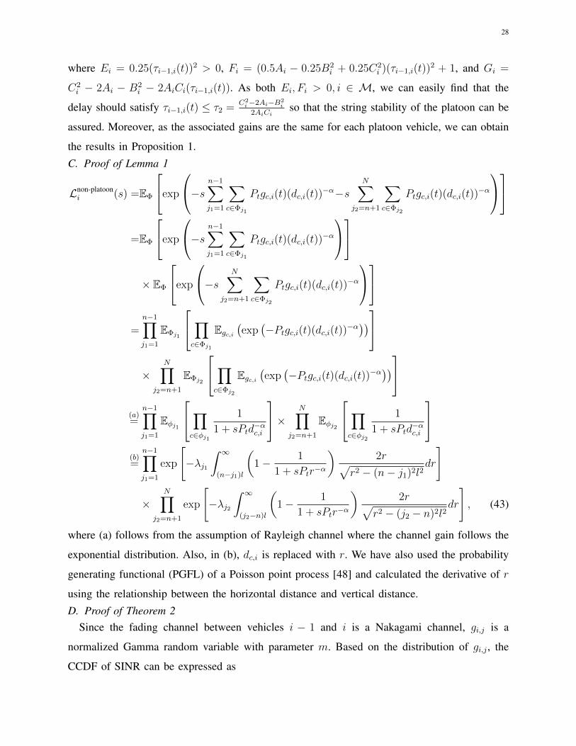
C. Proof of Lemma 1

Lnon-platooni (s) =EΦ

exp

−s n−1∑j1=1

∑c∈Φj1

Ptgc,i(t)(dc,i(t))−α−s

N∑j2=n+1

∑c∈Φj2

Ptgc,i(t)(dc,i(t))−α

=EΦ

exp

−s n−1∑j1=1

∑c∈Φj1

Ptgc,i(t)(dc,i(t))−α

× EΦ

exp

−s N∑j2=n+1

∑c∈Φj2

Ptgc,i(t)(dc,i(t))−α

=

n−1∏j1=1

EΦj1

∏c∈Φj1

Egc,i(exp

(−Ptgc,i(t)(dc,i(t))−α

))×

N∏j2=n+1

EΦj2

∏c∈Φj2

Egc,i(exp

(−Ptgc,i(t)(dc,i(t))−α

))(a)=

n−1∏j1=1

Eφj1

∏c∈φj1

1

1 + sPtd−αc,i

× N∏j2=n+1

Eφj2

∏c∈φj2

1

1 + sPtd−αc,i

(b)=

n−1∏j1=1

exp

[−λj1

∫ ∞(n−j1)l

(1− 1

1 + sPtr−α

)2r√

r2 − (n− j1)2l2dr

]

×N∏

j2=n+1

exp

[−λj2

∫ ∞(j2−n)l

(1− 1

1 + sPtr−α

)2r√

r2 − (j2 − n)2l2dr

], (43)

where (a) follows from the assumption of Rayleigh channel where the channel gain follows the

exponential distribution. Also, in (b), dc,i is replaced with r. We have also used the probability

generating functional (PGFL) of a Poisson point process [48] and calculated the derivative of r

using the relationship between the horizontal distance and vertical distance.

D. Proof of Theorem 2Since the fading channel between vehicles i − 1 and i is a Nakagami channel, gi,j is a

normalized Gamma random variable with parameter m. Based on the distribution of gi,j , the

CCDF of SINR can be expressed as

29

F(θ) =P(γi,j > θ) = P

(Ptgi,jd

−αi−1,i

σ2 + Inon-platooni (t) + Iplatoon

i (t)> θ

)

=P

(gi,j >

θ(σ2 + Inon-platooni (t) + Iplatoon

i (t))

Ptd−αi−1,i

)(a)≈1− EΦ∪Ψ

[(1− exp

(−ηθdαi−1,i(σ

2 + Inon-platooni (t) + Iplatoon

i (t))

Pt

))m](b)=

β∑k=1

(−1)k+1

(β

k

)EΦ∪Ψ

(exp

(−kηθdαi−1,i(σ

2 + Inon-platooni (t) + Iplatoon

i (t))

Pt

))

=

β∑k=1

(−1)k+1

(β

k

)exp

(−kηθdαi−1,i

Ptσ2

)EΦ

(exp

(−kηθdαi−1,i

PtInon-platooni (t)

))EΨ

(exp

(−kηθdαi−1,i

PtIplatooni (t)

))(c)=

β∑k=1

(−1)k+1

(β

k

)exp

(−kηθdαi−1,i

Ptσ2

)Lnon-platooni

(kηθdαi−1,i

Pt

)Lplatooni

(kηθdαi−1,i

Pt

),

(44)

where η = β(β!)−1β , (a) is based on the approximation of tail probability of a Gamma function

[49], (b) follows Binomial theorem and the assumption that m is an integer, and the changes in

(c) follow the definition of Laplace transform. Also, we can calculate the PDF of the SINR at

vehicle i as f(θ) = d(1−F(θ))dθ

= −F(θ)dθ

. Therefore, according to the relationship between the data

rate and SINR, we can obtain the mean and variance of service time in (19) and (20).E. Proof of Theorem 3

The first element in the maximization function is actually a lower bound for the reliability,

which is proven by

P(T1 + T2 ≤ min(τ1, τ2)) = 1− P(T1 + T2 ≥ min(τ1, τ2))

(a)

≥ 1− E(T1 + T2)

min(τ1, τ2)= 1− T1 + T2

min(τ1, τ2), (45)

where (a) is based on Markov’s inequality [50]. For the second element in the maximization

function, we leverage the Chernoff bound [51] in (a) to obtain another lower bound. Between

these two lower bounds, we can always choose the tighter bound to be closer to the reliability

of the wireless network, as shown in (23).F. Proof of Corollary 3

To prove Corollary 3, we first let τ3 = T1+T2min(τ1,τ2)

, 0 ≤ τ3 ≤ 1, and the two functions in the (37)

can be simplified as

30

1− T1 + T2

min(τ1, τ2)= 1− τ3, (46)

1−exp

(T1+T2−min(τ1, τ2) ln

(min(τ1, τ2)

T1 + T2

))= 1−exp

[(T1+T2)

(1− 1

τ3

ln(1

τ3

)

)], (47)

where both (46) and (47) are decreasing functions in terms of τ3. Note that finding the maximum

value between functions (46) and (47) is equivalent to maximizing the maximal value of (46)

and (47). Therefore, the solution is to minimize τ3, which equals to maximizing min(τ1, τ2). In

other words, the solutions for the optimization problem in (28)–(32) apply to the problem for

the reliability lower bounds as long as the solutions can guarantee T1 + T2 ≤ min(τ1, τ2).

REFERENCES

[1] T. Zeng, O. Semiari, W. Saad, and M. Bennis, “Integrated communications and control co-design for vehicular platoonsystems,” in Proc. of IEEE International Conference on Communication (ICC), Kansas City, MO, USA, May 2018.

[2] A. Ferdowsi, U. Challita, and W. Saad, “Deep learning for reliable mobile edge analytics in intelligent transportationsystems: An overview,” IEEE Vehicular Technology Magazine, vol. 14, no. 1, pp. 62–70, Mar. 2019.

[3] R. Hall and C. Chin, “Vehicle sorting for platoon formation: Impacts on highway entry and throughput,” TransportationResearch Part C: Emerging Technologies, vol. 13, no. 5-6, pp. 405–420, Oct.–Dec. 2005.

[4] K.-Y. Liang, J. Martensson, and K. H. Johansson, “Heavy-duty vehicle platoon formation for fuel efficiency,” IEEETransactions on Intelligent Transportation Systems, vol. 17, no. 4, pp. 1051–1061, Apr. 2016.

[5] C. Nowakowski, J. O’Connell, S. E. Shladover, and D. Cody, “Cooperative adaptive cruise control: Driver acceptance offollowing gap settings less than one second,” in Proc. of the Human Factors and Ergonomics Society Annual Meeting, LosAngles, CA, USA, Sept. 2010.

[6] C. Perfecto, J. Del Ser, and M. Bennis, “Millimeter-wave V2V communications: Distributed association and beamalignment,” IEEE Journal on Selected Areas in Communications, vol. 35, no. 9, pp. 2148–2162, Sept. 2017.

[7] I. G. Jin, S. S. Avedisov, and G. Orosz, “Stability of connected vehicle platoons with delayed acceleration feedback,” inProc. of ASME Dynamic Systems and Control Conference, Stanford, CA, USA, Oct. 2013.

[8] C. Bergenhem, S. Shladover, E. Coelingh, C. Englund, and S. Tsugawa, “Overview of platooning systems,” in Proc. ofITS World Congress, Vienna, Austria, Oct. 2012.

[9] Z. Xu, X. Li, X. Zhao, M. H. Zhang, and Z. Wang, “DSRC versus 4G-LTE for connected vehicle applications: A studyon field experiments of vehicular communication performance,” Journal of Advanced Transportation, vol. 2017, pp. 1–10,Aug. 2017.

[10] X. Liu, A. Goldsmith, S. S. Mahal, and J. K. Hedrick, “Effects of communication delay on string stability in vehicleplatoons,” in Proc. of Intelligent Transportation Systems, Oakland, CA, USA, Aug. 2001.

[11] H. Peng, D. Li, Q. Ye, K. Abboud, H. Zhao, W. Zhuang, and X. S. Shen, “Resource allocation for D2D-enabled inter-vehicle communications in multiplatoons,” in Proc. of IEEE International Conference on Communications (ICC), Paris,France, May 2017.

[12] P. S. Bithas, A. G. Kanatas, D. B. da Costa, P. K. Upadhyay, and U. S. Dias, “On the double-generalized gamma statisticsand their application to the performance analysis of V2V communications,” IEEE Transactions on Communications, vol. 66,no. 1, pp. 448–460, Jan. 2018.

[13] P. S. Bithas, A. G. Kanatas, D. B. da Costa, and P. K. Upadhyay, “Transmit antenna selection in vehicle-to-vehicletime-varying fading channels,” in Proc. of IEEE International Conference on Communications (ICC), Paris, France, May2017.

[14] X. Du, H. Zhang, H. Van Nguyen, and Z. Han, “Stacked lstm deep learning model for traffic prediction in vehicle-to-vehiclecommunication,” in Proc. of IEEE Vehicular Technology Conference (VTC-Fall), Toronto, Canada, Sept. 2017.

[15] J. Xu, L. Duan, and R. Zhang, “Surveillance and intervention of infrastructure-free mobile communications: A new wirelesssecurity paradigm,” IEEE Wireless Communications, vol. 24, no. 4, pp. 152–159, Aug. 2017.

[16] H. Peng, D. Li, K. Abboud, H. Zhou, H. Zhao, W. Zhuang, and X. S. Shen, “Performance analysis of ieee 802.11 p DCFfor multiplatooning communications with autonomous vehicles,” IEEE Transactions on Vehicular Technology, vol. 66,no. 3, pp. 2485–2498, Mar. 2017.

[17] Y. Hu, H. Li, Z. Chang, R. Hou, and Z. Han, “End-to-end backlog and delay bound analysis using martingale for internetof vehicles,” in Proc. of IEEE Conference on Standards for Communications and Networking (CSCN), Helsinki, Finland,Sept. 2017.

[18] R. Kaewpuang, D. Niyato, P.-S. Tan, and P. Wang, “Cooperative management in full-truckload and less-than-truckloadvehicle system,” IEEE Transactions on Vehicular Technology, vol. 66, no. 7, pp. 5707–5722, Jul. 2017.

31

[19] A. Vahidi and A. Eskandarian, “Research advances in intelligent collision avoidance and adaptive cruise control,” IEEEtransactions on intelligent transportation systems, vol. 4, no. 3, pp. 143–153, Sept. 2003.

[20] K. Li and P. Ioannou, “Modeling of traffic flow of automated vehicles,” IEEE Transactions on Intelligent TransportationSystems, vol. 5, no. 2, pp. 99–113, Jun. 2004.

[21] G. Orosz, “Connected cruise control: modelling, delay effects, and nonlinear behaviour,” Vehicle System Dynamics, vol. 54,no. 8, pp. 1147–1176, Aug. 2016.

[22] S. Lucero, “Cellular–vehicle to everything (C-V2X) connectivity,” IHS Technology, Internet Everything, vol. 3, June 2016.[23] J. G. Andrews, R. K. Ganti, M. Haenggi, N. Jindal, and S. Weber, “A primer on spatial modeling and analysis in wireless

networks,” IEEE Communications Magazine, vol. 48, no. 11, pp. 156–163, Nov. 2010.[24] Z. Gong and M. Haenggi, “Interference and outage in mobile random networks: Expectation, distribution, and correlation,”

IEEE Transactions on Mobile Computing, vol. 13, no. 2, pp. 337–349, Feb. 2014.[25] E. Yaacoub, F. Filali, and A. Abu-Dayya, “QoE enhancement of SVC video streaming over vehicular networks using

cooperative LTE/802.11 p communications,” IEEE Journal of Selected Topics in Signal Processing, vol. 9, no. 1, pp.37–49, Feb. 2015.

[26] E. A. Feukeu, K. Djouani, and A. Kurien, “Compensating the effect of doppler shift in a vehicular network,” in 2013Africon, Sep. 2013, pp. 1–7.

[27] R. He, A. F. Molisch, F. Tufvesson, Z. Zhong, B. Ai, and T. Zhang, “Vehicle-to-vehicle propagation models with largevehicle obstructions,” IEEE Transactions on Intelligent Transportation Systems, vol. 15, no. 5, pp. 2237–2248, Oct. 2014.

[28] L. Cheng, B. E. Henty, D. D. Stancil, F. Bai, and P. Mudalige, “Mobile vehicle-to-vehicle narrow-band channel measurementand characterization of the 5.9 ghz dedicated short range communication (DSRC) frequency band,” IEEE Journal onSelected Areas in Communications, vol. 25, no. 8, Oct. 2007.

[29] G. Acosta-Marum and M. Ingram, “Doubly selective vehicle-to-vehicle channel measurements and modeling at 5.9 GHz,”in Proc. International Symposium Wireless Personal Multimedia Communication, San Diego, CA, USA, Sept. 2006.

[30] M. Bando, K. Hasebe, A. Nakayama, A. Shibata, and Y. Sugiyama, “Dynamical model of traffic congestion and numericalsimulation,” Physical review E, vol. 51, no. 2, p. 1035, Feb. 1995.

[31] D. Swaroop and J. K. Hedrick, “String stability of interconnected systems,” IEEE Transactions on Automatic Control,vol. 41, no. 3, pp. 349–357, Mar. 1996.

[32] G. A. Baker, Essentials of Pade approximants. Academic Press, 1975.[33] Y. Chen, “Mathematical modelling of end-to-end packet delay in multi-hop wireless networks and their applications to qos

provisioning,” Ph.D. dissertation, UCL (University College London), 2013.[34] Y. Yang, M. Shao, S. Zhu, B. Urgaonkar, and G. Cao, “Towards event source unobservability with minimum network

traffic in sensor networks,” in Proc. of ACM conference on Wireless network security, Alexandria, VA, USA, Mar. 2008.[35] D. Shuman and M. Liu, “Optimal sleep scheduling for a wireless sensor network node,” in Proc. of IEEE Asilomar

Conference on Signals, Systems and Computers, Pacific Grove, CA, USA, Oct. 2006.[36] L. Kleinrock, Queueing systems, volume 1: Theory. Wiley New York, 1976.[37] P. J. Burke, “The output of a queuing system,” Operations research, vol. 4, no. 6, pp. 699–704, Dec. 1956.[38] P. G. Harrison and N. M. Patel, Performance modelling of communication networks and computer architectures. Addison-

Wesley Longman Publishing Co., Inc., 1992.[39] W. Yu and R. Lui, “Dual methods for nonconvex spectrum optimization of multicarrier systems,” IEEE Transactions on

Communications, vol. 54, no. 7, pp. 1310–1322, Jul. 2006.[40] S. Boyd and L. Vandenberghe, Convex optimization. Cambridge university press, 2004.[41] Berkeley highway lab website. [Online]. Available: http://bhl.path.berkeley.edu[42] S. Panichpapiboon and L. Cheng, “Irresponsible forwarding under real intervehicle spacing distributions,” IEEE Transac-

tions on Vehicular Technology, vol. 62, no. 5, pp. 2264–2272, Jun. 2013.[43] X. Ma, X. Chen, and H. H. Refai, “Performance and reliability of dsrc vehicular safety communication: a formal analysis,”

EURASIP Journal on Wireless Communications and Networking, vol. 2009, no. 1, pp. 1–13, Jan. 2009.[44] J. B. Kenney, “Dedicated short-range communications (DSRC) standards in the United States,” Proceedings of the IEEE,

vol. 99, no. 7, pp. 1162–1182, Jul. 2011.[45] I. G. Jin and G. Orosz, “Dynamics of connected vehicle systems with delayed acceleration feedback,” Transportation

Research Part C: Emerging Technologies, vol. 46, pp. 46–64, Sept. 2014.[46] K. Liu, G. Xie, and L. Wang, “Consensus for multi-agent systems under double integrator dynamics with time-varying

communication delays,” International Journal of Robust and Nonlinear Control, vol. 22, no. 17, pp. 1881–1898, Sept.2011.

[47] K. Gu, J. Chen, and V. L. Kharitonov, Stability of time-delay systems. Springer Science & Business Media, 2003.[48] M. Haenggi, Stochastic geometry for wireless networks. Cambridge University Press, 2012.[49] T. Bai and R. W. Heath, “Coverage and rate analysis for millimeter-wave cellular networks,” IEEE Transactions on Wireless

Communications, vol. 14, no. 2, pp. 1100–1114, Feb. 2015.[50] E. M. Stein and R. Shakarchi, Real analysis: measure theory, integration, and Hilbert spaces. Princeton University Press,

2009.[51] W. Hoeffding, “Probability inequalities for sums of bounded random variables,” Journal of the American statistical

association, vol. 58, no. 301, pp. 13–30, Mar. 1963.