Joint ICTP-IAEA Workshop on Nuclear Reaction Data for...

1944-17

Joint ICTP-IAEA Workshop on Nuclear Reaction Data for AdvancedReactor Technologies

J.M. Kendall

19 - 30 May 2008

Global Virtual LLCPrescot t

U S A

Critical Experiments and Reactor Physics Calculations for Low-EnrichedHigh Temperature Gas Cooled Reactors.

IAEA TECDOC 1249 (advance electronic version)

Critical Experiments and Reactor

Physics Calculations for Low-Enriched

High Temperature Gas Cooled Reactors

The originating Section of this publication in the IAEA was:

Nuclear Power Technology Development Section International Atomic Energy Agency

Wagramer Strasse 5 P.O.Box 100

A-1400 Vienna, Austria

Critical Experiments and Reactor Physics Calculations for Low-Enriched High Temperature Gas Cooled Reactors

IAEA, Vienna, 2001 IAEA-TECDOC--1249

advance electronic copy © IAEA, 2001

FOREWORD

An important function of the International Atomic Energy Agency is to "foster the exchange of

scientific and technical information" and to "encourage and assist research on, and development

and practical application of, atomic energy for peaceful uses throughout the world". For

innovative advanced nuclear reactor concepts, IAEA Member States in many cases find it

attractive to cooperate internationally in technology development. The IAEA's gas-cooled

reactor technology development activities, which are conducted within its Nuclear Power

Program, encourage international cooperation through technical information exchange and

cooperative research.

Advanced gas cooled reactor designs currently under development are predicted to achieve a

high degree of safety through reliance on innovative features and passive systems. The IAEA's

activities in this field during the 1990’s focused on three technical areas that are essential to

providing this high degree of safety, but which must be proven. These technical areas are:

(a) the neutron physics behavior of the reactor core

(b) the ability of ceramic coated fuel particles to retain the fission products, even under extreme

accident conditions

(c) the ability of the designs to dissipate decay heat by natural transport mechanisms

To enhance confidence in predictions of neutron physics behavior, the IAEA established a

Coordinated Research Project (CRP) on Validation of Safety Related Physics Calculations for

Low Enriched HTGRs. Countries participating in this CRP include China, France, Japan,

Switzerland, Germany, the Netherlands, the USA and the Russian Federation. Its objective was

to fill gaps in validation data for physics methods used for core design of gas-cooled reactors

fueled with low enriched uranium. Within this CRP, an international team of researchers was

assembled at the PROTEUS critical experiment facility of the Paul Scherrer Institute, Villigen,

Switzerland, to plan, conduct and analyze a new series of critical experiments focused on the

needs of participating countries. In this CRP, experience from critical experiment programs in

the Russian Federation and Japan was also utilized.

The following institutes participated in this CRP:

Paul Scherrer Institute (PSI), Villigen, Switzerland

Institute for Nuclear Energy Technology (INET), Tsinghua University, Beijing, China

Forschungzentrum Jülich (FZJ), Jülich, Germany

Japan Atomic Energy Research Institute (JAERI), Tokai-mura, Japan

Interfaculty Reactor Institute, Delft University, Delft, the Netherlands

Centre d'Etudes de Cadarache (CEA), St. Paul les Durance-Cedex, France

Oak Ridge National Laboratory (ORNL), Oak Ridge, USA

Russian Research Center Kurchatov Institute (RRC-KI), Moscow, Russia

Energy Research Center, Petten, the Netherlands

General Atomics (GA), San Diego, USA

Experimental Machine Building Design Bureau (OKBM), Nizhny Novgorod, Russia

This report was edited by T. Williams and M. Rosselet (formerly PSI), and W. Scherer (FZJ) .

The IAEA project officers for the CRP were J. Cleveland and H. Brey, and the officer

responsible for this publication was J. Kendall. Additional CRPs addressing technical areas (b)

and (c) were conducted in parallel, with results documented in IAEA TECDOCs 978 and 1163.

CONTENTS

1. INTRODUCTION.............................................................................................................. 1

2. SAFETY RELATED PHYSICS VALIDATION DATA AND NEEDS FOR

ADVANCED GAS-COOLED REACTOR DESIGNS................................................... 2

2.1 PHYSICS VALIDATION DATA NEEDS FOR ADVANCED GCRS............................. 2 2.2 SUMMARY OF VALIDATION DATA BASE (PRIOR TO CRP)................................... 7 2.3 PLANNING OF PROTEUS EXPERIMENTS TO PROVIDE VALIDATION DATA..13

3. EARLY PROBLEM ANALYSIS................................................................................... 17

3.1 PROTEUS..................................................................................................................... 17 3.2 VHTRC..........................................................................................................................30

4. PROTEUS CRITICAL EXPERIMENT FACILITY................................................... 46

4.1 HISTORY OF THE FACILITY AND RECONFIGURATION FOR THE HTR EXPERIMENTS........................................................................................................... 46

4.2 HTR-PROTEUS FACILITY DESCRIPTION.............................................................. 47

5. PROTEUS EXPERIMENT PLANS...............................................................................58

6. PROTEUS MEASUREMENT TECHNIQUES............................................................ 63

6.1 CRITICAL LOADINGS............................................................................................... 63 6.2 REACTIVITY MEASUREMENTS..............................................................................65 6.3 KINETIC PARAMETER (β/Λ).................................................................................... 86 6.4 REACTION-RATE MEASUREMENTS......................................................................90 6.5 GRAPHITE ABSORPTION MEASUREMENTS........................................................99

7. PROTEUS EXPERIMENTAL RESULTS.................................................................. 105

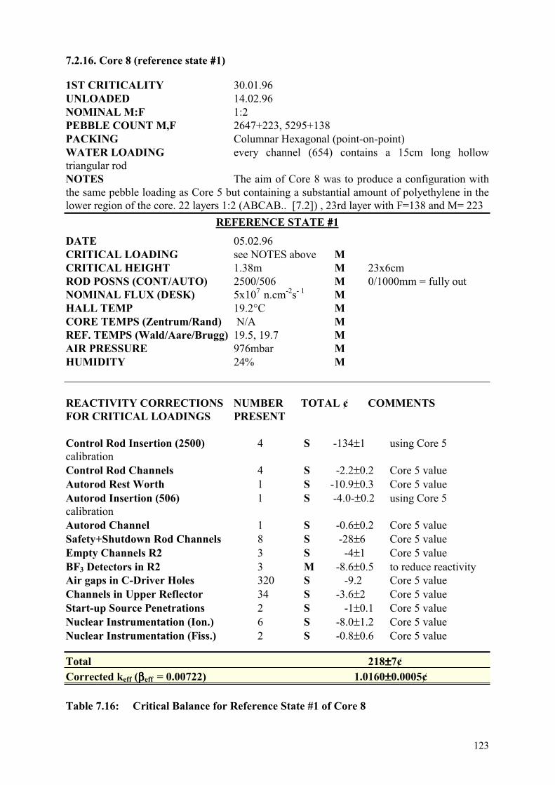
7.1. INTRODUCTION....................................................................................................... 105 7.2 CRITICAL BALANCE............................................................................................... 106 7.3 INTEGRAL AND DIFFERENTIAL CONTROL ROD WORTHS........................... 127 7.4 SHUTDOWN ROD WORTHS................................................................................... 133 7.5 KINETIC PARAMETER (βeff/Λ)............................................................................... 137 7.6 OTHER INTEGRAL PARAMETERS....................................................................... 143

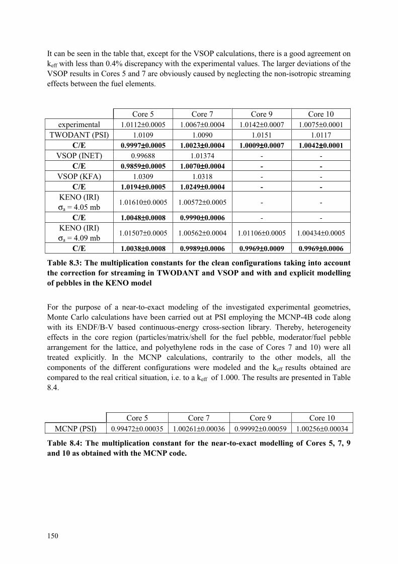
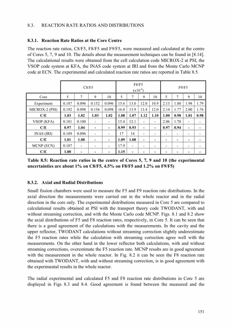
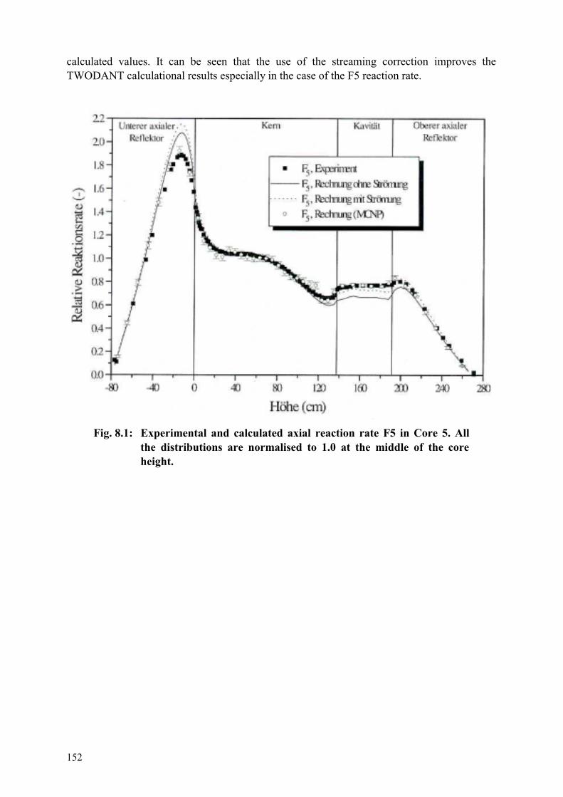
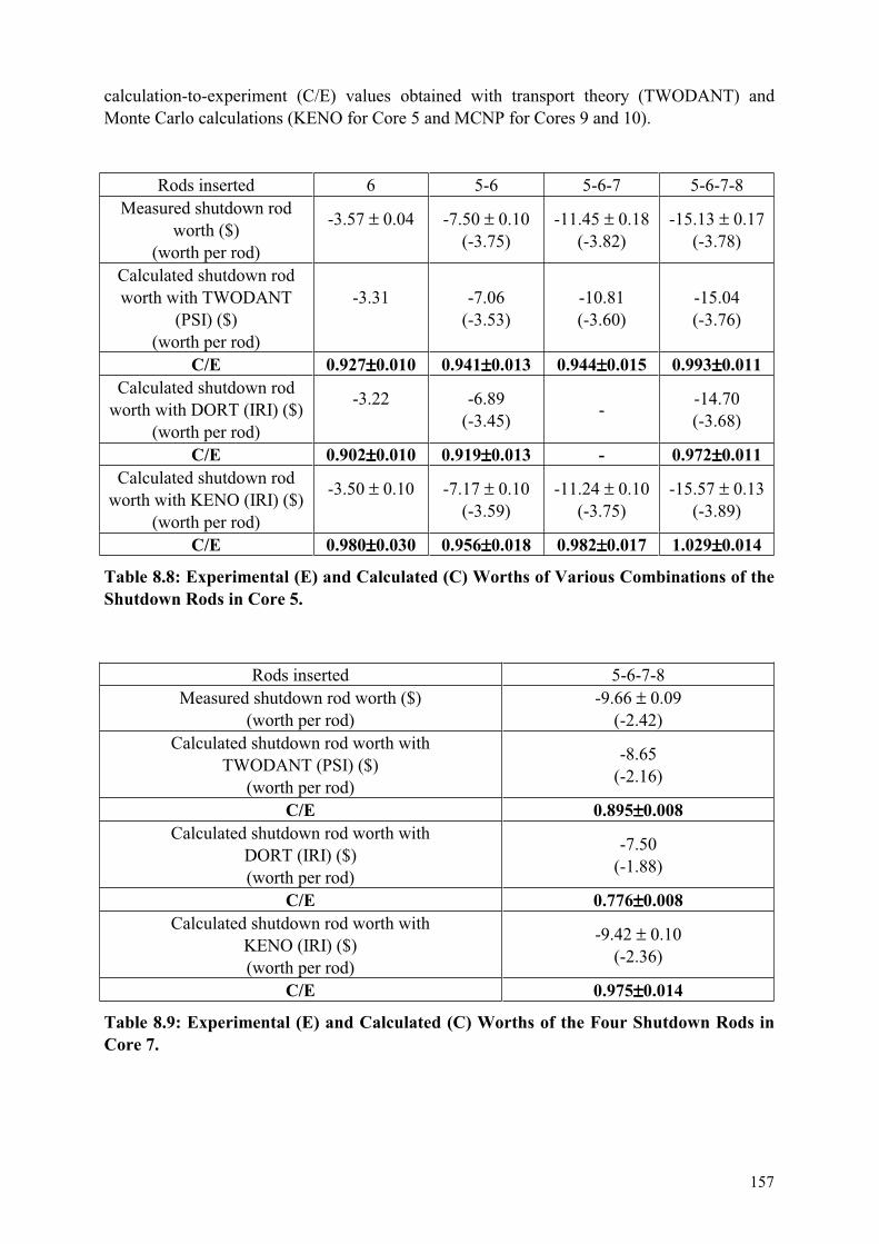
8. COMPARISON OF MEASUREMENTS WITH CALCULATIONS.......................145

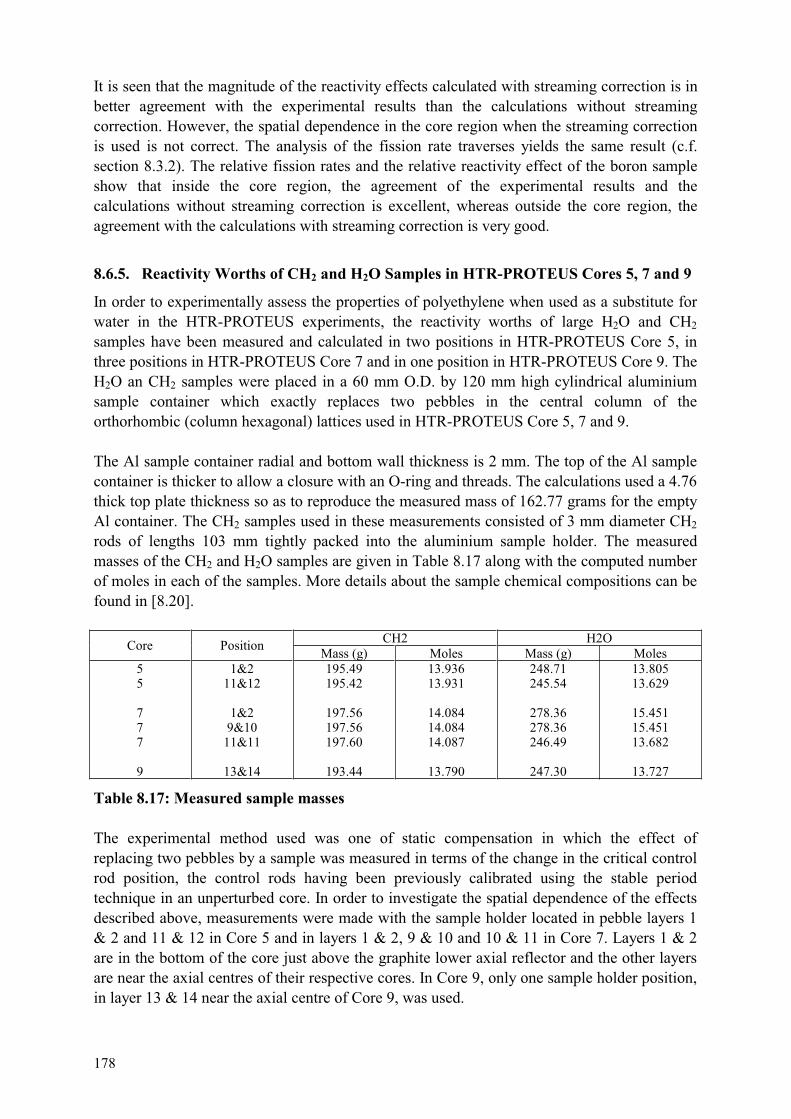
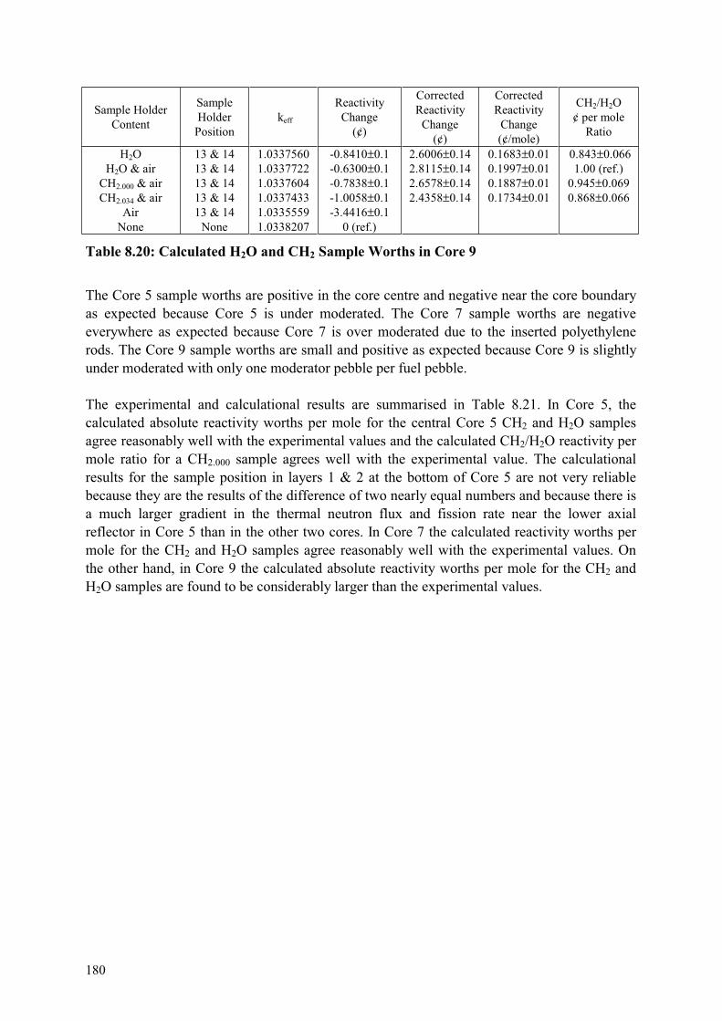
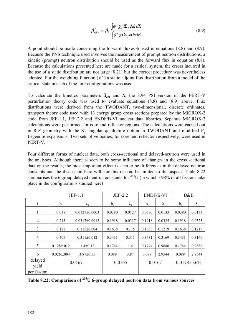
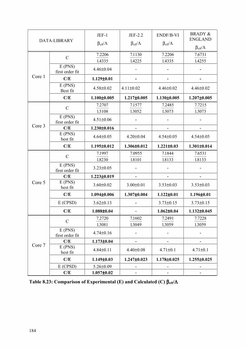
8.1 INTRODUCTION....................................................................................................... 145 8.2 CRITICAL BALANCES INCLUDING STREAMING............................................. 145 8.3 REACTION RATE RATIOS AND DISTRIBUTIONS............................................. 151 8.4 CONTROL ROD WORTHS....................................................................................... 154 8.5 WATER INGRESS EFFECTS....................................................................................162 8.6 REACTIVITY OF SMALL SAMPLES......................................................................168 8.7 KINETIC PARAMETER............................................................................................ 181

9. SUMMARY AND CONCLUSIONS......................................................................………189

9.1 LEU-HTR PROTEUS PROGRAM. ..............…........................................................ 189 9.2 BENCHMARK CALCULATIONS............................................................................ 190 9.3 PROTEUS EXPERIMENTAL PROCEDURES...................................................…..191 9.4 COMPARISON OF MEASUREMENTS WITH CALCULATIONS........................ 194

APPENDIX A. ASSIGNMENT OF RESEARCHERS FROM PARTICIPATING

INSTITUTES TO THE PROTEUS TEAM.............................................. 197

APPENDIX B. EXTERNAL PUBLICATIONS MADE IN CONNECTION WITH

HTR PROTEUS........................................................................................ 200

APPENDIX C. QUALITY ASSURANCE PLAN FOR THE HTR-PROTEUS

EXPERIMENTS.................................................................203

1

1. INTRODUCTION

On the recommendation of the International Atomic Energy Agency's International Working Group on Gas Cooled Reactors, the IAEA established a Coordinated Research Project (CRP) on the Validation of Safety Related Physics Calculations for Low-Enriched High Temperature Gas Cooled Reactors (HTGRs) in 1990. The objective of the CRP was to provide safety-related physics data for low-enriched uranium (LEU) fueled HTGRs for use in validating reactor physics codes used by the participating countries for analyses of their designs. Experience on low-enriched uranium, graphite-moderated reactor systems from research institutes and critical facilities in participating countries were brought into the CRP and shared among participating institutes.

The status of experimental data and code validation for HTGRs and the remaining needs at the initiation of this CRP were addressed in detail at the IAEA Specialists Meeting on Uncertainties in Physics Calculations for HTGR Cores [1.1] which was hosted by the Paul Scherrer Institute (PSI), Villigen, Switzerland in May of 1990.

The main activities of the CRP were conducted within an international project at the PROTEUS critical experiment facility at the Paul Scherrer Institute, Villigen, Switzerland. Within this project, critical experiments were conducted for graphite moderated LEU systems to determine core reactivity, flux and power profiles, reaction-rate ratios, the worth of control rods, both in-core and reflector based, the worth of burnable poisons, kinetic parameters, and the effects of moisture ingress on these parameters. Fuel for the experiments was provided by the KFA Research Center, Jülich, Germany. Initial criticality was achieved on July 7, 1992. These experiments were conducted over a range of experimental parameters such as carbon-to-uranium ratio, core height-to-diameter ratio, and simulated moisture concentration. To assure that the experiments being conducted are appropriate for the designs of the participating countries, specialists from each of the countries have participated in planning the experiments. Several of the participating countries also sent representatives to PSI to participate in the conduct of the experiments, as listed in Appendix A.

In addition, to the PROTEUS experiments, data from the LEU fueled critical experiments at the Japanese VHTRC critical experiment facility on the temperature coefficient (to 200°C) are of interest for physics code validation and were analyzed by CRP participants.

This report summarizes the existing base of information for validation of core physics design codes at the time that the CRP was initiated, describes the cooperative activities conducted within the CRP, provides information on the PROTEUS facility and the results of the critical experiments conducted, and summarizes the results of the validation activities conducted by the participants.

REFERENCES

[1.1] Proceedings of an IAEA Specialists Meeting on Uncertainties in Physics Calculations for Gas-cooled Reactor Cores, Villigen, Switzerland, May 1990, IWGGCR/24, IAEA Vienna, 1991.

2

2. SAFETY RELATED PHYSICS VALIDATION DATA AND NEEDS FOR ADVANCED

GAS-COOLED REACTOR DESIGNS

Advanced gas-cooled reactors currently being developed are predicted to achieve a simplification of safety and licensing requirements through reliance on innovative features and passive systems. Specifically, this simplification derives from a combination of

a) the neutron physics behavior of the reactor core b) reliance on ceramic coated fuel particles to retain the fission products even under extreme

accident conditions c) the ability to dissipate decay heat by natural transport mechanisms without reaching excessive

fuel temperatures d) the resistance of the fuel and reactor core to chemical attack (air or water ingress).

Development activities in several countries have focused on the validation of these features under experimental conditions representing realistic reactor conditions. It is important to note that validation of these features was identified as a key requirement by the U.S. Nuclear Regulatory Commission in the draft Safety Evaluation Report for the modular HTGR [2.1].

2.1. PHYSICS VALIDATION DATA NEEDS FOR ADVANCED GCRS

Innovative features employed by advanced gas cooled reactors vary according to the specific design, but include the following features, which reactor core physics codes should be able to treat with sufficient accuracy:

- LEU fuel - control rods located both in the core and in the side reflector - annular core - large H/D ratio of core

Further, particularly for steam cycle concepts, the design codes must be able to accurately predict the effect of moisture ingress into the core on key safety parameters.

Tables 2.1a-d present the important core-physics parameters and the desired conditions for validation data for the design of advanced gas-cooled reactors in several participating countries. These requirements were developed early in the CRP and can be expected to change somewhat with time as designs evolve.

3

Parameter Desired conditions

Core criticality

• Fissile and fertile particles in cylindrical fuel rods • LEU / Natural U fuel • Core average C / fissile atom ratio: - 3900 at BOEC *

- 6500 at EOEC *

• Reload 235U enrichment: - 19.8 wt. % in fissile particles - 15.5 wt % in fissile + fertile particles • Average 235U enrichment in both particles - 13.0 wt. % at BOEC*

- 8.6 wt. % at EOEC*

• Effects of cylindrical B4C poison rods

Temperature coefficient • To high temperature, i.e. to 1000 °C or above, if possible • Reflector contribution • Effects of moisture

Control rod worth • B4C control rods in side reflector and core • Effects of moisture

Power distribution • Effects of control rods in the reflector • Effects of partly inserted control rods

Water ingress • Effect on reactivity, temperature coefficient, and control rod worth

• Range of interest for the average water density in the active core of the GT-MHR is up to 0.009 g/cm3 for hot conditions, and up to 0.053 g/cm3 for cold conditions.

Decay heat LEU / natural U fuel

Reactor transients LEU / natural U fuel

Reactor shielding Neutron fluence on reactor vessel, and its spectral distribution

* BOEC = Beginning of Equilibrium Cycle

EOEC = End of Equilibrium Cycle

Table 2.1a Advanced gas-cooled reactor physics validation needs for U.S. GT-MHR

4


Core criticality

• LEU • C / 235U atom ratio 7000 • 8% 235U enrichment

Temperature coefficient • to high temperature • effect of water ingress • reflector contribution • Pu effects

Control rod worth • B4C control rods in side reflector and core • tall, high leakage, cylindrical core • effect of water

Burnable poison worth • B4C

Neutron flux and power distribution

• tall, high leakage, cylindrical core • effect of reflector control rods on power distribution • effect of partly inserted rods • fluence on reactor vessel, and its spectral distribution

Water ingress effects • on reactivity • on temperature coefficient • on control rod worth

Table 2.1b Advanced gas-cooled reactor physics validation needs for the

Russian VGM

5


Core criticality • LEU (18% 235U enrichment) • BOC C / 235U ratio = 4000 • EOC C / 235U ratio = 10000 • with no control rods in core or nearby reflector • core height 1.76m, core diameter 1.90m • stochastic effects • streaming effects

Temperature coefficient • to high temperatures • around room temperature also useful

Control rod worth • close to core (6cm) • effect of moisture

Burnable poison worth • pebbles with 4.2g hafnium and 40mg boron • effect of moisture • effect of a layer of absorber pebbles on top of core

Water ingress • especially around 7kg per cubic meter in core

Neutron balance components • reaction rate ratios


• desirable

Other • reactivity effect of nitrogen in core • reactivity effect of fuel pebbles in discharge pipe • reactivity effect of fuel pebbles in different positions

Table 2.1c Advanced gas-cooled reactor physics validation needs for HTR-10 (China)

- adopted from [2.2]

6


Core criticality • LEU • C/U atom ratio 450 to 650 (1000 also desirable) • 7 to 10 % 235U enrichment

Temperature coefficient • from ambient to high temperature • effect of moisture/steam • reflector influence • Pu effects

Control rod worth • B4C control rods in side reflector • small B4C absorber spheres (KLAK) • small core, high leakage • influence of moisture/steam


• small, tall core geometry • effect of partly inserted reflector rods • fluence on reactor vessel

Water ingress effects • reactivity as function of H2O concentration • effect of inhomogeneous H2O distribution • influence on control rod / KLAK reactivity • influence on power distribution • influence on temperature coefficient

(The water density range of interest is up to equivalent 70 bar saturated steam to cover hypothetical accident scenarios)

TABLE 2.1d Advanced gas-cooled reactor physics validation needs for Germany

(HTR modul)

7

2.2. SUMMARY OF VALIDATION DATA BASE (PRIOR TO CRP)

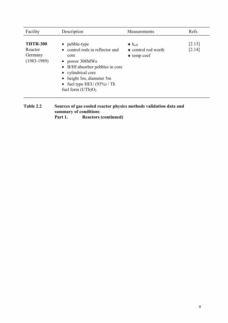
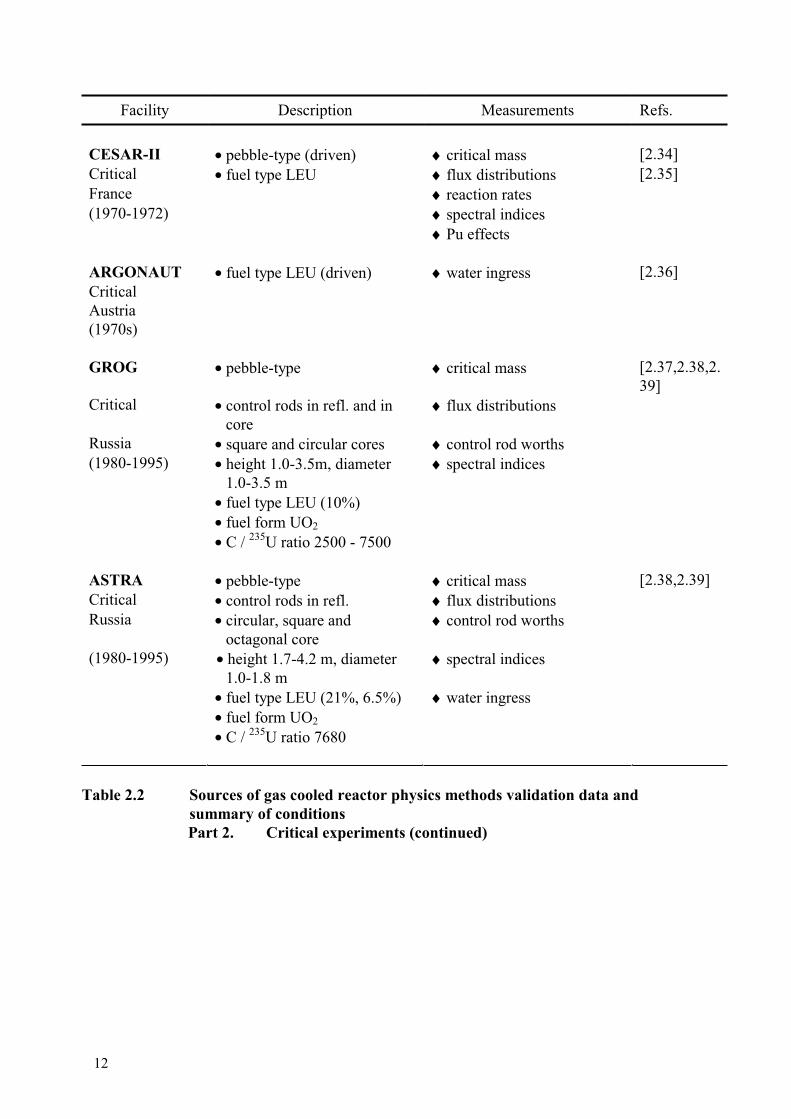
The adequacy of computational methods used to compute safety-related physics parameters for advanced gas cooled reactors must be supported by comparisons with experimental data covering an appropriate range of conditions. Validation data is available from power reactors as well as past critical experiments. These are listed in Table 2.2, along with a summary of experimental conditions and references to reports providing more detailed information. Note that most of the existing validation data is for HEU/Th fueled systems.

8

Facility Description Measurements Refs.

Dragon • block-type ♦ keff [2.3,2.4] Reactor • control rods in reflector ♦ control rod worthUK • power 20 MWth ♦ power distributions(1964-75) • hexagonal core ♦ temp coef./defect [2.5]

• height 1.6m, diameter 1.1m • fuel type HEU (93%) / Th • fuel form UC2 -ThC2

Peach Bottom • graphite rod fuel type ♦ keff

Reactor • control rods in core ♦ power distributionsUSA • power 115 MWth ♦ control rod worth [2.6] (1967-75) • cylindrical core ♦ temp coef./defect (to 730°C

• height 2.3m, diameter 2.7m outlet gas temperature.) • fuel type HEU (93%) / Th • fuel form U3O8

• reload C / 235U ratio 2000 • B4C burnable poison

Fort St Vrain • block-type ♦ keff [2.7] Reactor • control rods in core ♦ power distributions [2.8] USA • power 842 MWth ♦ control rod worth [2.9] (1974-89) • cylindrical core ♦ temp coef./defect (to 730°C

• height 4.8m, diameter 5.9m outlet gas temperature) • fuel type HEU (93%) / Th • fuel form UCO • reload C / 235U ratio 3000

AVR • pebble-type ♦ keff [2.10] Reactor • control rods in ‘noses’ ♦ control rod worthGermany • power 46 MWth ♦ temp coef. (cold and hot) [2.11] (1966-88) • cylindrical core ♦ pebble flow patterns

• height 2.8m, diameter 3.0m ♦ Pu build-up measurements • fuel type HEU (93%) / Th ♦ reactivity / temp. transients [2.12]

and LEU • reload C / 235U ratio 3770 • fuel form (UTh)O2,(UTh)C2

Table 2.2 Sources of gas cooled reactor physics methods validation data and

summary of conditions

Part 1. Reactors

9


THTR-300 • pebble-type ♦ keff [2.13] Reactor Germany

• control rods in reflector and core

♦ control rod worth♦ temp coef

[2.14]

(1983-1989) • power 308MWe • B/Hf absorber pebbles in core • cylindrical core • height 5m, diameter 5m • fuel type HEU (93%) / Th

fuel form (UTh)O2



Part 1. Reactors (continued)

10


Peach Bottom • block-type ♦ keff [2.15] Critical • control rods in core ♦ control rod worth [2.16] USA • cylindrical core ♦ power distributions(1959-62) • height 1.2m, diameter 1.5m ♦ temp coef./defect

• fuel type HEU (93%) / Th ♦ water ingress • fuel form U3O8

• C / 235U ratio 2775 HTLTR • block-type ♦ temp coef./defect [2.17] Critical • control rods in core [2.18] USA • cubic core (1970-71) • height 3.0m, width 1.5m

• fuel type Pu&HEU (93%)/Th • fuel form UC2-ThO2 & U3O8

• C / 235U ratio 5710 HTGR • block-type ♦ keff [2.16] Critical • control rods in core ♦ control rod worth [2.19] USA • rectangular core, split table ♦ temp coef./defect [2.20] (1966-69) • height 1.8m, width 2.1m

• fuel type HEU (93%)/Th • fuel form U3O8

• C / 235U ratio 2680 HITREX-2 • block-type ♦ keff [2.21] Critical • control rods in core and refl. ♦ control rod worth [2.22] USA • hexagonal core ♦ power distributions(1971-75) • height 2.0m, diameter 2.5m

• fuel type LEU (3.5%) • fuel form UO2

• C / 235U ratio 10300



Part 2. Critical experiments

11


CNPS • block-type ♦ keff [2.23] Critical • control rods in core ♦ control rod worthUSA • cylindrical core ♦ temp coef./defect (1987-89) • height 1.1m, diameter 1.2m ♦ water ingress

• fuel type LEU (20%) • fuel form UCO • C / 235U ratio 3000

SHE • block-type (split-table) ♦ keff [2.24] Critical • various core shapes ♦ control rod worth [2.25] Japan • height 2.4m, diameter 2.4m ♦ temp coef. at 700°C [2.26] (1975-1985) • fuel type LEU (20%) ♦ flux distributions [2.27]

• fuel form UO2

• C / 235U ratio 2000-16000 VHTRC • block-type (split-table) ♦ keff [2.28] Critical • control rods in core ♦ keff with burnable poison Japan • hexagonal core ♦ control rod worths in core (1985-1995) • height 2.4m, diameter 2.4m and reflector

• fuel type LEU (2, 4, 6 %) ♦ temp. coef (up to 200°C) [2.29] • fuel form UO2 ♦ flux distributions • C / 235U ratio 8800-17500 ♦ water ingress

♦ kinetic parameter (βeff/Λ)♦ βeff [2.30]

KAHTER • pebble-type ♦ keff [2.31] Critical • control rods in core and refl. ♦ control rod worths in core [2.32] Germany • cylindrical core and reflector [2.33] (1973-75) • height 2.8m, diameter 2.2m ♦ flux distributions

• fuel type HEU (93%) / Th ♦ water ingress???? • fuel form (UTh)O2

• C / 235U ratio 7550



Part 2. Critical experiments (continued)

12


CESAR-II • pebble-type (driven) ♦ critical mass [2.34] Critical • fuel type LEU ♦ flux distributions [2.35] France ♦ reaction rates (1970-1972) ♦ spectral indices

♦ Pu effects ARGONAUT • fuel type LEU (driven) ♦ water ingress [2.36] Critical Austria (1970s) GROG • pebble-type ♦ critical mass [2.37,2.38,2.

39] Critical • control rods in refl. and in

core♦ flux distributions

Russia • square and circular cores ♦ control rod worths (1980-1995) • height 1.0-3.5m, diameter

1.0-3.5 m ♦ spectral indices

• fuel type LEU (10%) • fuel form UO2

• C / 235U ratio 2500 - 7500 ASTRA • pebble-type ♦ critical mass [2.38,2.39] Critical • control rods in refl. ♦ flux distributions Russia • circular, square and

octagonal core ♦ control rod worths

(1980-1995) • height 1.7-4.2 m, diameter 1.0-1.8 m

♦ spectral indices

• fuel type LEU (21%, 6.5%) ♦ water ingress • fuel form UO2

• C / 235U ratio 7680



Part 2. Critical experiments (continued)

13

2.3. PLANNING OF PROTEUS EXPERIMENTS TO PROVIDE VALIDATION DATA

The PROTEUS graphite moderated LEU critical experiments were planned to fill gaps in the base of validation data. The constraints included room temperature and 5500 LEU fuel pebbles supplied by the KFA Research Center, Jülich, Germany. Specifically, the experiments which could be conducted at the PROTEUS facility with the available AVR LEU fuel are summarized in Table 2.3.

___________________________________________________________________________________• clean critical cores • LEU pebble-type fuel with 16.76% U235 enrichment • a range of C/U atom ratio of 946 to 1890 (achieved by varying the moderator-to-fuel pebble ratio from

0.5 to 2.0) • core (equivalent) diameter = 1.25 m • core height = 0.843 m to 1.73 m (with simulated water ingress smaller core heights are possible) • core H/D from 0.7 to 1.4 • flux distribution measurements and spectral distribution measurements (including measurements in

side reflector) • kinetic parameter measurements • worth of reflector control rods (partly and fully inserted) • worth of in-core control rod (partly and fully inserted) • effects of moisture ingress over range of water density up to 0.25 gm H2O/cm3 void (corresponds to

0.065 gm H2O/cm3 core for PROTEUS). Water is simulated with polyethylene inserts. ♦ effect on core reactivity ♦ effect on worth of reflector control rods ♦ effect on worth of in-core control rod ♦ effect on burnable poison worth ♦ effect on prompt neutron lifetime ♦ effect on flux and power distributions

_____________________________________________________________________________________

Table 2.3 Summary of PROTEUS critical experiments

PROTEUS results fill certain gaps in required experimental data for code validation for advanced gas-cooled reactors which are under development. Comparing the data needs (from Table 2.1) with the experimental conditions achievable at PROTEUS (from Table 2.3) demonstrates the following:

• The PROTEUS criticals provide validation data for low-enriched uranium fuel with an enrichment near to that planned for advanced GCR designs.

• PROTEUS moisture ingress experiments will investigate the effects which are important for advanced GCR designs (i.e., reactivity worth of moisture, and the effect of moisture on control rod and burnable poison worth and on reaction rate distributions) over the range of moisture densities of interest.

• The achievable range of C/U atom ratio at PROTEUS is near to, but higher than that of advanced GCR designs (this ratio is an important factor in determining the neutron energy spectrum).

• PROTEUS provides validation data − for the worth of reflector control rods − for the worth of an in-core control rod− for the worth of small samples of burnable poison (B4C) − for fission rate distributions in core and reflector.

14

REFERENCES

[2.1] WILLIAMS, P.M., KING, T.L., WILSON, J.N., ”Draft Preapplication Safety Evaluation Report for the Modular High Temperature Gas-cooled Reactor”, NUREG-1338, U.S. Nuclear Regulatory Commission, 1989

[2.2] LUO, J., “The INET 10MW HTR Test Module and Possibilities for its Physics Design Validation in PROTEUS”, PSI Internal Report TM-41-90-29, Aug. 1990.

[2.3] DELLA LOGGIA, V. E. et al., “Zero Energy Experiments on the Dragon Reactor Prior to Charge IV Startup”, DP820, Dragon Project, AEEW, Winfrith, UK, Jan. 1973

[2.4] DELLA LOGGIA, V. E. et al., “Measurements of Control Rod Worth and Excess Reactivity on the First Core of Dragon”, DP359, Dragon Project, AEEW, Winfrith, UK, July 1965

[2.5] DELLA LOGGIA, V. E. et al., “Zero Power Measurement of the Temperature Coefficient of the DRAGON Core”, DP402, Dragon Project, AEEW, Winfrith, UK, May 1966

[2.6] BROWN, J.R., PRESKITT, C.A., NEPHEW, E.A., VAN HOWE, K.R., ”Interpretation of Pulsed-source Experiments in the Peach Bottom HTGR”, Nucl. Sci.

& Eng., 29, 283, (1967)

[2.7] BROWN, J. R. et al., “Physics Testing at Fort St. Vrain - A Review”, Nucl. Sci. &

Eng., 97, 104, (1987)

[2.8] MARSHALL, A. C., and BROWN, J. R., ”Neutron Flux Distribution Measurements in the Fort St. Vrain Initial Core”, GA-A13176, General Atomics, San Diego, Feb. 1975

[2.9] BROWN, J.R., PFEIFFER, W., MARSHALL, A.C., “Analysis and Results of Pulsed-neutron Experiments Performed on the Fort St. Vrain High Temperature Gas-Cooled Reactor”, Nucl. Tech., 27, 352, (1975)

[2.10] KIRCH, N., IVENS, G., “Results of AVR Experiments”, in “AVR-Experimental High-Temperature Reactor: 21 Years of Successful Operation for a Future Energy Technology”, Assoc. of German Engineers (VDI) -The society for energy technologies (1989)

[2.11] POHL, P., et al., “Determination of the Hot- and Cold- Temperature Coefficient of Reactivity in the AVR Core”, Nucl. Sci. & Eng., 97, 64, (1987)

[2.12] SCHERER, W., et al., “Analysis of Reactivity and Temperature Transient Experiments at the AVR High Temperature Reactor”, Nucl. Sci. & Eng., 97, 58, (1987)

[2.13] BRANDES, S., et al., “Core Physics Tests of High Temperature Reactor Pebble Bed at Zero Power”, Nucl. Sci. & Eng., 97, 89, (1987)

[2.14] SCHERER, W., et al., “Adaptation of the Inverse Kinetic Method to Reactivity Measurements in the Thorium High-temperature Reactor-300”, Nucl. Sci. & Eng., 97,58, (1987)

[2.15] BROWN, J.R., DRAKE, M.K., VAN HOWE, K.R., ”Correlation of calculations and Experimental Measurements Made Using a Partial Core Mockup of the Peach Bottom HTGR”, GA-3799, General Atomics, San Diego, Mar. 1963

15

[2.16] BARDES, R.G. et al., ”Results of HTGR Critical Experiments Designed to Make Integral Checks on the Cross Sections in Use at Gulf General Atomic”, GA-8468, General Atomics, San Diego, Feb. 1968

[2.17] NEWMAN, D.F., “Temperature-dependent k-infinity for a ThO2 -PuO2 HTGR Lattice (HTLTR)”, Nucl. Technol., 19, (1973)

[2.18] OAKES, T.J., ”Measurement of the Neutron Multiplication Factor as a Function of Temperature for a 235UC2-

232ThO2-C Lattice (HTLTR)”, BNWL-SA-3621, 1973.

[2.19] MATHEWS, D.R., ”Reanalysis of the HTGR Critical Control Rod Experiments”, GA-A13739, General Atomics, San Diego, Nov. 1975

[2.20] NIRSCHL, R.J., GILLETTE, E.M., BROWN, J.R., ”Experimental and analytical Results for HTGR Type Control Rods of Hafnium and Boron in the HTGR Critical Facility”, Gulf-GA-A-9354, General Atomics, San Diego, Jan 1973

[2.21] KITCHING, S.J., et al., ”Physics Measurements on the Zero-Energy Reactor HITREX-2 Incorporating an Integral Block Fuel Zone: Description of the Programme and stage 1 Measurements on the basic Lattices”, RD/B/N3979, Jan 1978

[2.22] McKECHNIE, A.J., ”An Analysis of Reactor Physics Experiments on the Basic Lattice of the BNL Reactor HITREX-2”, RD/B/N4580, June 1979

[2.23] HANSEN, G.E., PALMER R.G., “Compact Nuclear Power Source Critical Experiments and Analysis”, Nucl. Sci. & Eng., 103, 237, (1989)

[2.24] KANEKO, Y., et al., ”Critical Experiments on Enriched Uranium Graphite moderated Cores”, JAERI 1257, June 1978

[2.25] KANEKO, Y., et al., ”Measurement of Multiple Control Rods Reactivity Worths in Semi-Homogeneous Critical Assembly”, JAERI-M 6549, May 1976

[2.26] YASUDA, H., et al., ”Measurement of Doppler Effect of Coated Particle Fuel Rod in SHE-14 Core Using Sample Heating Device”, J. Nucl. Sci & Technol., 24, 6 (1987)

[2.27] AKINO, F., et al., ”Measurement of Neutron Flux Distributions in Graphite-moderated Core SHE-8 with Inserted Experimental Control Rods”, JAERI-M 6701, Sept. 1976

[2.28] AKINO, F., YAMANE, T., YASUDA, H., KANEKO, Y., ”Critical Experiments at Very High Temperature Reactor Critical Assembly (VHTRC)”, Proc. Int. Conf. on the

Physics of Reactors - Physor '90, Marseilles, France, 13-26 April 1990.

[2.29] YAMANE, T. et al., ”Measurement of Overall Temperature Coefficient of Reactivity of VHTRC-1 Core by Pulsed Neutron Method”, J. Nucl. Sci. & Technol., 27, 2 , (1990)

[2.30] AKINO, F. et al., ”Measurement of the Effective Delayed Neutron Fraction for VHTRC-1 Core”, To be published in J. Nucl. Sci. & Technol..

[2.31] DRÜCKE, V. et al., ”The Critical HTGR Test Facility KAHTER - An Experimental Program for Verification of Theoretical Models, Codes and Nuclear Design Bases”, Nucl. Sci. & Eng, 97, 30 (1987)

[2.32] SCHERER, W. et al., ”Theoretische Analyse des kritischen HTR-Experimentes KAHTER”, Jül-1136-RG, Nov. 1974

[2.33] SÜSSMANN, H.F., et al., ”Reaktivitätsbestimmung an der graphit-moderierten Kritischen Anlage KAHTER mittels Rauschanalyse”, Jül-1368, 1976

16

[2.34] SCHERER, W. et al., ”Das kritische HTR Experiment CESAR-II; ein Test der Aussagekraft neutronphysikalischer Berechnungen zur Auslegung von Hochtemperaturreaktoren”, Jül-975-RG, 1973

[2.35] SCHAAL, H., ”Entwicklung eines Rechenverfahrens zur Bestimmung von effektiven Plutonium-Wirkungsquerschnitten in niedrig angereicherten HTR-Gittern und Test am Experiment CESAR-2”, Jül-1757 (1982)

[2.36] SCHÜRRER, F. et al., ”Überprüfung transporttheoretischer Methoden zur Neutronenfluss- und Kritikalitätsbestimmung für den Störfall des Wassereinbruchs in gasgekühlte Kugelhaufenreaktoren”, Reaktor-Institute Graz, RIG-19, 1986)

[2.37] BOGOMOLOV A.M., KAMINSKY A.S., PARAMONOV V.V. et. al., “Main Characteristics of GROG Critical Facility and Problem of HTGR Physics Study”, VANT issues Atomic-Hydrogen Energy and Technology, 3(10), Moscow, ISSN 0206-4960 p.p. 17-21 (1981)

[2.38] BAKULIN S.V., GARIN V.P., Ye.S.GLUSHKOV E.S. et.al., “Study of HTGR Nuclear Criticality Safety at the GROG and ASTRA Facilities”, Proceedings of the Fifth International Conference on Nuclear Criticality Safety, ICNC ‘95. Albuquerque, NM USA, September 17-21, 1995, p.p. 6.18-6.24

[2.39] GLUSHKOV E.S., DAVIDENKO V.D., KAMINSLY A.S. et.al., “Physical Characteristics of the Critical Assemblies with Spherical Fuel Elements”, VANT issues Nuclear Reactor Physics and Calculational Methods, 1, Kurchatov Institute, Moscow, ISSN 0205-4671, p.p. 62-72 (1992)

17

3. EARLY PROBLEM ANALYSIS

This chapter summarizes code results for two calculation exercises proposed to the various participants as an early problem analysis. The first was to perform core calculations on six proposed configurations for the PROTEUS LEU-HTR critical experiments. Unit cell parameters such as kinf for both an infinite spectrum and the spectrum corresponding to critical buckling as well as migration length are cross-compared. For the whole core calculations, parameters reported include keff, critical height and neutron balance. In addition, spectral indices estimated by the different codes for both unit cells and whole cores are also included for cross-comparison. The second exercise involved a temperature coefficient benchmark calculation by code participants, mocking up heating experiments conducted by JAERI on their pin-in-block type critical assembly, VHTRC. Both unit cell parameters and whole core criticality and temperature coefficients are reported as function of temperature. The latter are compared to experimental results

3.1. PROTEUS

3.1.1. Introduction

Calculational benchmark problems based on some of the initially proposed configurations for the LEU-HTR critical experiments in the PROTEUS facility were prepared and distributed by PSI to the organizations in the CRP in 1990 [3.1.1]. The benchmarks consist of six graphite-reflected 16.76% enriched-uranium pebble-bed systems of three different lattice geometries and two different moderator-to-fuel pebble ratios (2:1 and 1:2).

3.1.2. Description

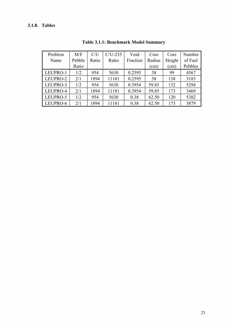
These benchmark problems were named LEUPRO-1 through LEUPRO-6. • LEUPRO-1 and -2 have a packing fraction of 0.7405 (hexagonal closed packed lattice). • LEUPRO-3 and -4 have a packing fraction of 0.6046 (columnar hexagonal lattice geometry). • LEUPRO-5 and -6 have a packing fraction of 0.6200 (stochastic -random- lattice geometry). A brief summary of the calculational models is given in Table 3.1.1.

A two-dimensional (R-Z) geometry representation of the PROTEUS critical facility was specified for these problems which are inherently two-dimensional in nature due to the relatively large void space between the pebble-bed core and the upper axial reflector in most of the problems. The effective core radii vary with the pebble packing factor due to the use of lattice geometry dependent graphite spacers between the core and the radial reflector. The graphite radial reflector is about 100 cm thick. The graphite axial reflectors are about 80 cm thick. The core cavity which is partly or fully filled with moderator and fuel pebbles is 173 cm high.

The core heights given in Table 3.1.1 were specified on the basis of preliminary two-dimensional (R-Z), discrete ordinates transport theory criticality calculations performed at PSI using JEF-1 nuclear data. The graphite reflector cross sections were incorrect in these preliminary PSI calculations. This error had a larger effect on the under-moderated systems than in the better moderated benchmarks. As a result, whole reactor eigenvalues significantly greater than unity are to be expected for the LEUPRO-1, -3 and -5 benchmarks. The core heights were

18

adjusted to yield an integral number of layers of pebbles except for LEUPRO-4 and -6 in which the maximum physically available core cavity height of 173 cm was specified.

3.1.3. Requested Results

Calculated results were requested for both unit cells and for the whole reactor.

For the unit cells the following parameters were requested: • kinf (0) for B2=0, i.e. production/absorption for B2=0,• the critical buckling B2

cr and k inf (B2cr),

• the migration area M2,• the spectral indices rho-28 (ρ 28 ), delta-25 (δ 25 ), delta-28 (δ 28 ) and C * ,

where: ρ 28 =C8epi/C8ther : ratio of epithermal-to-thermal 238U captures δ 25 =F5epi/F5ther : ratio of epithermal-to-thermal 235U fissions δ 28 =F8/F5 : ratio of fissions in 238U to fissions in 235U

C * =C8/F5 : ratio of captures in 238U to fissions in 235U

Double-heterogeneity of the fuel pebbles was to be taken into account, i.e. self-shielding of the fuel grains in the fuel pebble, as well as the self-shielding of the pebbles in the lattice. In addition, results obtained considering only a single-heterogeneity of the unit cell, i.e. without grain self-shielding, as well as results for a fully homogeneous core (no grain or pebble self-shielding) were requested for the LEUPRO-1 benchmark only. Finally results for the LEUPRO-1 benchmark modified to add 20v/o water in the void space between the pebbles were requested.

For the whole reactor the following results were requested: • keff for the specified dimensions and specified atomic densities, • the critical pebble-bed core height Hcr,• the spectral indices at core center and core averaged, • neutron balance in terms of absorption, production and leakage, integrated over the pebble-

bed core region.

3.1.4. Participants

The following nine institutes from seven countries participated in the benchmark • The Institute of Nuclear Energy Technology (INET) in China • The KFA Research Center Jülich (KFA) in Germany • The Japan Atomic Energy Research Institute HTTR Group (JAERI-HTTR) in Japan • The Japan Atomic Energy Research Institute VHTRC Group (JAERI-VHTRC) in Japan • The Netherlands Energy Research Foundation (ECN) in The Netherlands • The Interfaculty Reactor Institute, Delft University of Technology (IRI) in The Netherlands • The Kurchatov Institute (KI) in Russia • The Paul Scherrer Institute (PSI) in Switzerland • The Oak Ridge National Laboratory (ORNL) in the USA

19

3.1.5. Methods and Data

Nearly all of the participants used different code systems and different nuclear data libraries. The MCNP Monte Carlo code was used by both ECN and ORNL and the VSOP code system was used by both INET and KFA, albeit with different nuclear data libraries. The whole reactor calculations used cross sections derived from the corresponding unit cell calculations unless otherwise noted.

3.1.5.1. Unit Cell Calculations

At ECN, unit cell results were obtained with the WIMS-E version 5a, the SCALE-4 and the MCNP codes. Cross-section data based on the JEF-2.2 evaluation were used in all these codes. The JEF-2.2 based WIMS-E library was the 172-group 1986 WIMS library. The SCALE-4 and MCNP cross section libraries were generated at ECN. The 172 group XMAS structure was used for the SCALE-4 library. MCNP used a continuous energy library prepared from the JEF-2.2 evaluation. With MCNP, the approximately 10,000 fuel grains surrounded by coating layers contained in each fuel pebble were explicitly modeled using a deterministic cubic fuel grain lattice geometry. The double-heterogeneity is thereby taken into account explicitly in the MCNP computations. The Dancoff factors needed to take the double-heterogeneity into account in SCALE-4 were also calculated with special MCNP calculations.

At INET, the ZUT-DGL, GAM and THERMOS models of the VSOP code system were used with an ENDF/B-IV based nuclear data library.

At IRI, unit cell calculations were obtained with the INAS (IRI-NJOY-AMPX-SCALE) system and the JEF-1.1 evaluated library. The Dancoff factors to take the double-heterogeneity into account were computed with DANCOFF-MC, a separate program based on the Monte Carlo Method.

At KFA, VSOP, AMPX and MUPO calculations were performed. The modules ZUT-DGL, GAM and THERMOS of the code system VSOP were used. The AMPX calculations used the NITAWL and XSDRN modules with a nuclear data library mostly based on ENDF/B-III ('old library') and ENDF/B-V and JEF-1 ('New Library'). The MUPO calculations used a forty three energy group data set which was developed for the German THTR-300 core calculations.

The JAERI-HTTR group used the code system DELIGHT with an ENDF/B-IV based nuclear data library.

At JAERI, the VHTRC group used the SRAC code system with an ENDF/B-IV based nuclear data library.

At KI, the unit cell results were obtained with the modules BIBCOT and BIBROT of the code system KRISTALL with an unspecified nuclear data library. Results were also obtained with the unit cell code FLY using 100 energy groups.

At ORNL, the calculations were done with MCNP version 4.x and an ENDF/B-V based nuclear data library. The double-heterogeneity explicitly taken into account in the ORNL MCNP computations

20

PSI used the code MICROX-2 and a JEF-1 based nuclear data library. Alternative nuclear data sets for graphite, 235U and 238U based on JEF-2.2 and ENDF/B-VI were prepared with NJOY. The use of the alternative data sets did not yield significantly different keff results. Significant delayed neutron data differences were observed [3.1.2].

3.1.5.2. Whole Reactor Calculations

At ECN, WIMS-E 5a, WIMS-6 and MCNP calculations were performed. The WIMS-E 5a calculations used the 69 group 1986 library to prepare a region dependent 10 group cross section data set for the two-dimensional R-Z diffusion theory SNAP module. WIMS-6 used the 172 group 1994 XMAS (JEF-2.2 based) data library to prepare a 10 group set for SNAP. One-dimensional radial and axial fine group calculations were performed to obtain space dependent spectra for condensing to 10 groups. A streaming correction was not done.

The ECN MCNP4a calculations used a continuous energy data library based on JEF-2.2. In the MCNP (R-Z) geometric model, the reactor core was filled with explicitly modeled fuel and moderator pebbles to the prescribed height and the fuel grains within each fuel pebble were also explicitly modeled. In this MCNP model, streaming of the neutrons between pebbles is explicitly taken into account.

At INET, the whole reactor calculations were done with the CITATION diffusion theory code. Four energy groups were used in R-Z geometry. The upper cavity was treated according the procedure developed by Gerwin and Scherer. Streaming corrections were not mentioned.

At IRI, the BOLD-VENTURE finite difference diffusion theory code in 4 energy groups was used. The geometry was R-Z with separate material zones for core, axial reflector, radial reflector, aluminum structure and void. No special treatment for the voided region was done, except that the diffusion coefficient was limited to 100 cm. Streaming correction was not taken into account.

The JAERI-VHTRC group used the two-dimensional R-Z TWOTRAN discrete ordinate transport theory code with 24 energy groups. A P0 Legendre expansion and S6 angular quadrature were used.

The JAERI-HTTR group used the CITATION 1000 VP diffusion theory code with 13 energy groups in R-Z geometry.

At KFA, whole reactor results were obtained with the CITATION diffusion theory code in R-Z geometry. Region dependent 4 energy groups were prepared. The diffusion coefficients for the upper cavity region were obtained from the special procedure developed by Gerwin and Scherer. Streaming corrections according to Lieberoth and Stojadinovic were used [3.1.3] and included in the final results.

At KI, the multi-dimensional numerical transport theory code KRISTALL was used with 5 energy groups. No streaming corrections were mentioned. A possible reduction in keff by 0.7% for LEUPRO-1 due to streaming was mentioned in a separate communication.

21

At ORNL MCNP-4.x calculations with an ENDF/B-V based cross sections library were performed. As in the ECN model, the fuel and moderator pebbles as well as the fuel grains in the fuel pebbles were explicitly modeled. The ORNL results therefore include neutron streaming.

At PSI results were obtained with the TWODANT discrete ordinates transport theory code in 13 energy groups. A modified P1 Legendre expansion and S6 angular quadrature were used in R-Z geometry. No streaming corrections were included.

3.1.6. Benchmark Results

The benchmark specification was provided by PSI, who also performed the compilation of the results. Beginning in 1991 results were presented by INET, JAERI-HTTR, JAERI-VHTRC, KFA, KI, ORNL and PSI. Since 1993, results from ECN and IRI have also become available. The results as of June 1996 were compiled by Mathews [3.1.4]. Additional results from ECN and KFA were presented at the 7-th CRP in Vienna on 26-28 November 1996.

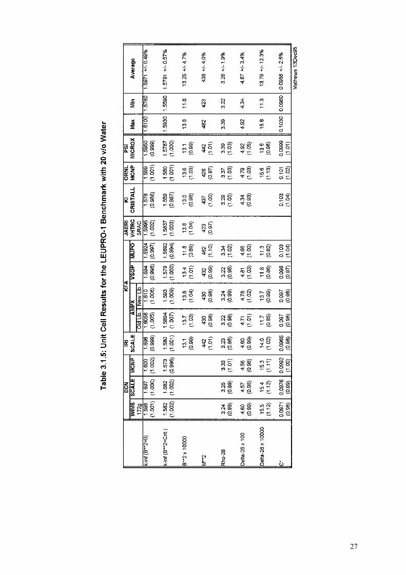
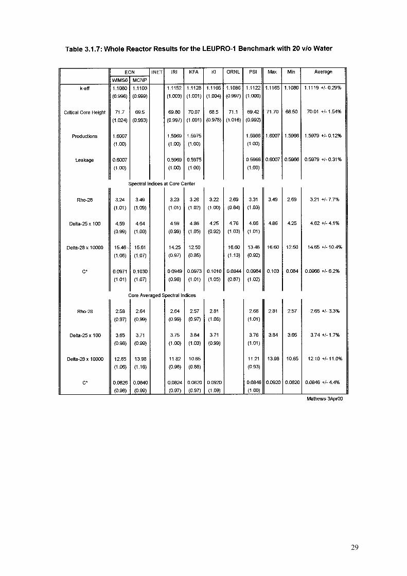
Results for the LEUPRO-1 benchmark only are given in this TECDOC. The results for the other benchmarks show similar trends. Table 3.1.2 gives unit cell results and Table 3.1.6 gives whole reactor results for the basic LEUPRO-1 benchmark situation. Table 3.1.5 and 3.1.7 give unit cell and whole reactor results respectively, for the LEUPRO-1 case with 20v/o of water between the pebbles. Tables 3.1.6 and 3.1.7 have been updated to include the November 1996 MCNP results from ECN. Table 3.1.3 gives unit cell results for the singly heterogeneous case (no grain self-shielding) and Table 3.1.4 gives unit cell results for the corresponding fully homogeneous version of the LEUPRO-1 benchmark.

Maxima, minima, arithmetic averages and one standard deviation (1σ) values in percent for the reported values are given in the right-hand columns of the tables. The numbers in parentheses in the tables are the ratio of the calculated value just above it to the average value for that quantity given in the right-most column of that row of the table.

The tables show a considerable spread of the results of the contributing laboratories, especially in the spectral indices.

A problem with the doubly-heterogeneous Dancoff factor of 0.13117 provided in the PSI benchmark specification for the LEUPRO-2, -4 and -6 configurations was noted by ECN and IRI and confirmed by KFA. The correct Dancoff factor for these configurations is about 0.23 instead of 0.13. The PSI results were not affected because the MICROX-2 unit cell code uses as input only singly-heterogeneous Dancoff factors which were correct in the benchmark specification.

3.1.7. Analysis of code results

• The kinf and keff values agree much better with each other than the spectral indices, indicating either the possibility of compensating errors in the eigenvalue calculations or the deliberate

22

choice of methods and data for routine calculations that do not give much attention to the reactions which do not significantly affect the computation of kinf and keff.

• For the unit cells and at the reactor core center, the δ 28 spectral index (ratio of fissions in 238U to fissions in 235U) results are particularly discrepant between the various laboratories. However, only about 0.2% of all fissions occur in 238U which means that the impact of variations in this quantity on the reported kinf and keff values is negligible.

• The next most discrepant spectral index (for the core averaged spectra, however, the most discrepant index) is δ 25 (ratio of epithermal-to-thermal 235U fissions). The percentage of fission in 235U occurring above 0.625 eV is about 10% in the under-moderated LEUPRO-1 benchmark and about 6% in the better moderated LEUPRO-2 benchmark, which means that the impact of variations in this quantity on the reported kinf and keff values is not very large.

• The important spectral index C* (ratio of captures in 238U to fissions in 235U) is generally well predicted.

• The spectral indices from the unit cell calculations were originally believed not to differ greatly from the core center results of the whole-reactor calculations. The reported results, however, show considerable variation in this respect, particularly the δ 28 spectral index. This means that the LEU-HTR PROTEUS core is not large enough to provide a central zone free from the influence of the reflectors, at least in the energy range of importance for fission in 238U.

• The keff results from the whole reactor calculations agree slightly better with each other (have a smaller relative standard deviation) than the unit cell results for kinf. This is not an expected result because of the presence of neutron streaming corrections of the same magnitude as the relative standard deviations of the keff values in the KFA, ORNL and ECN (MCNP) whole reactor keff results which systematically lower these keff values as compared with the other whole reactor results and should cause larger deviations. Exclusion of the particularly discrepant KI (FLY) and KFA (MUPO) unit cell results (these methods were not used in the whole reactor results) would lead to the expected result.

REFERENCES

[3.1.1] MATHEWS, D., CHAWLA, R., ”LEU-HTR PROTEUS Calculational Benchmark Specifications”, PSI Technical Memorandum TM-41-90-32 (9 Oct. 1990)

[3.1.2] WILLIAMS, T., “On the Choice of Delayed Neutron Parameters for the Analysis of Kinetics Experiments in 235U Systems,” Ann. Nucl. Energy Vol. 23, No. 15 (1996) pp1261-1265

[3.1.3] LIEBEROTH, J., STOJADINOVIC, A., “Neutron Streaming in Pebble Beds,” Nucl. Sci. & Eng. 76 (1980) p336

[3.1.4] MATHEWS, D., ”Compilation of IAEA-CRP Results for the LEU-HTR PROTEUS Calculational Benchmarks”, PSI Technical Memorandum TM-41-95-28 (21 Jun. 1996)

23

3.1.8. Tables

Table 3.1.1: Benchmark Model Summary

ProblemName

M/F PebbleRatio

C/U Ratio

C/U-235Ratio

VoidFraction

Core Radius(cm)

Core Height (cm)

Numberof Fuel Pebbles

LEUPRO-1 1/2 954 5630 0.2595 58 99 4567 LEUPRO-2 2/1 1894 11181 0.2595 58 138 3183 LEUPRO-3 1/2 954 5630 0.3954 59.85 132 5294 LEUPRO-4 2/1 1894 11181 0.3954 59.85 173 3469 LEUPRO-5 1/2 954 5630 0.38 62.50 120 5382 LEUPRO-6 2/1 1894 11181 0.38 62.50 173 3879

24

25

26

27

28

29

30

3.2. VHTRC

3.2.1. Introduction

A “VHTRC Temperature Coefficient Benchmark Problem” was proposed by JAERI at the second Research Co-ordination Meeting (RCM) of the CRP held in Tokai, Japan 1991 [3.2.1]. These benchmark specifications were made on the basis of assembly heating experiments in the pin-in-block type critical assembly, VHTRC, in which the core is loaded with low enriched uranium, coated particle type fuel. From the viewpoint of HTR neutronics, the VHTRC benchmark is complementary to the LEU-HTR PROTEUS calculational benchmark [3.2.2] which was loosely based upon the planned PROTEUS experiments which were of course carried out at ambient temperatures.

This benchmark problem is intended to be useful for the validation of:

(1) Evaluated nuclear data for low enriched uranium-graphite systems

(2) Calculation of effective multiplication factor

(3) Calculation of temperature coefficient in a low temperature range

3.2.2. Benchmark Description

The VHTRC benchmark problem consists of two parts: VH1-HP and VH1-HC. VH1-HP requires the determination of the temperature coefficient of reactivity for five temperature steps between 20°C and 200°C. VH1-HC on the other hand requires the determination of the effective multiplication factor for two temperature states at which the core is nearly critical. The requested items are the cell parameters, effective multiplication factor, temperature coefficient of reactivity, reaction rates, fission rate distributions and effective delayed neutron fraction. Complete descriptions of the problems are given in the published document [3.2.3].

3.2.3. System Description

The VHTRC is a graphite moderated critical assembly which has a core loaded with pin-in-block fuel of low enriched uranium and a graphite reflector. The general arrangement of the critical assembly is shown in Figure 3.2.1. Fuel rods are inserted in holes of the graphite blocks. Fuel compacts in a fuel rod are made of coated fuel particles uniformly dispersed in the graphite matrix.

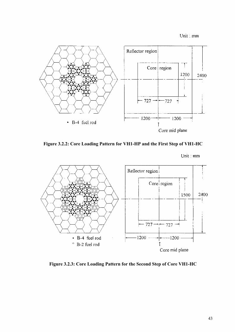
In the experiments corresponding to the benchmark problem, the assembly was first brought to a critical state at room temperature (see Figure 3.2.2). The assembly was then heated stepwise by using electric heaters up to 200 °C. At each step, the assembly temperature was kept constant so that an isothermal condition was realised, and subcritical reactivity was measured by the pulsed neutron method. Descriptions of the experiment upon which this benchmark problem, VHI-HP, was based can be found in [3.2.4]. At 200 °C, criticality was again attained by fuel rod addition and control rod adjustment (see Figure 3.2.3) (the B-2 and B-4 fuel rods contain 2 and 4 wt% enriched U-235, respectively). Descriptions of the experiment upon which the VH1-HC benchmark was based can be found in [3.2.5].

31

3.2.4. Methods and Data

The following seven institutes from five countries participated in the benchmark

• The Institute of Nuclear Energy Technology (INET) in China

• The KFA Research Centre Jülich (KFA) in Germany

• The Japan Atomic Energy Research Institute (JAERI) in Japan

• The Experimental Machine Building Design Bureau (OKBM) in Russia

• The Kurchatov Institute (KI) in Russia

• General Atomics (GA) in the USA

• The Oak Ridge National Laboratory (ORNL) in the USA

Each institute analyzed the problem by applying a calculation code system and data used for HTR development in his particular country, see Table 3.2.1 for a summary of the codes and data used.

The nuclear data used in the benchmark analyses were mostly based on the ENDF/B-IV or ENDF/B-V files with some additional use of ENDF/B-III and JEF-1 also being made. Russian institutes used their domestic nuclear data files for which details were not specified. The OKBM also used the UKNDL data for comparison with their original analysis route. Some of the institutes whose nuclear data libraries were not prepared at the temperatures specified in the benchmark, obtained their results by interpolation and extrapolation from calculations at temperatures available in the libraries.

Cell calculations were performed with a variety of codes, all considering double heterogeneity of the VHTRC fuel. Resonance absorption was treated by hyper-fine group calculations. There were some differences in the geometric models, for instance, some institutes used a fully cylindrical model whereas others used a combined hexagonal/cylindrical model. The ORNL calculations used a continuous energy Monte Carlo code (MCNP) and assumed that the fuel particles were arranged in a cubic lattice within an infinite two-dimensional hexagonal cell.

In the whole reactor calculations, most institutes used multi-group diffusion theory codes with different neutron energy group structures. The number of neutron energy groups ranged from two to twenty-five. In the preparation of few-group constants, particular attention was paid to the neutron energy spectrum in the small VHTRC system, characterized as it is by high neutron leakage. The three institutes of INET, KFA and KI introduced the buckling recycle technique for this reason. The ORNL carried out continuous energy MCNP calculations at a fixed temperature (300K) for a rigorous treatment of the actual reactor geometry, again with the simplification of a cubic lattice of fuel particles within the fuel rods.

3.2.5. Results

Calculational results are summarized in the compilation report [3.2.6], from which the following general findings were extracted.

32

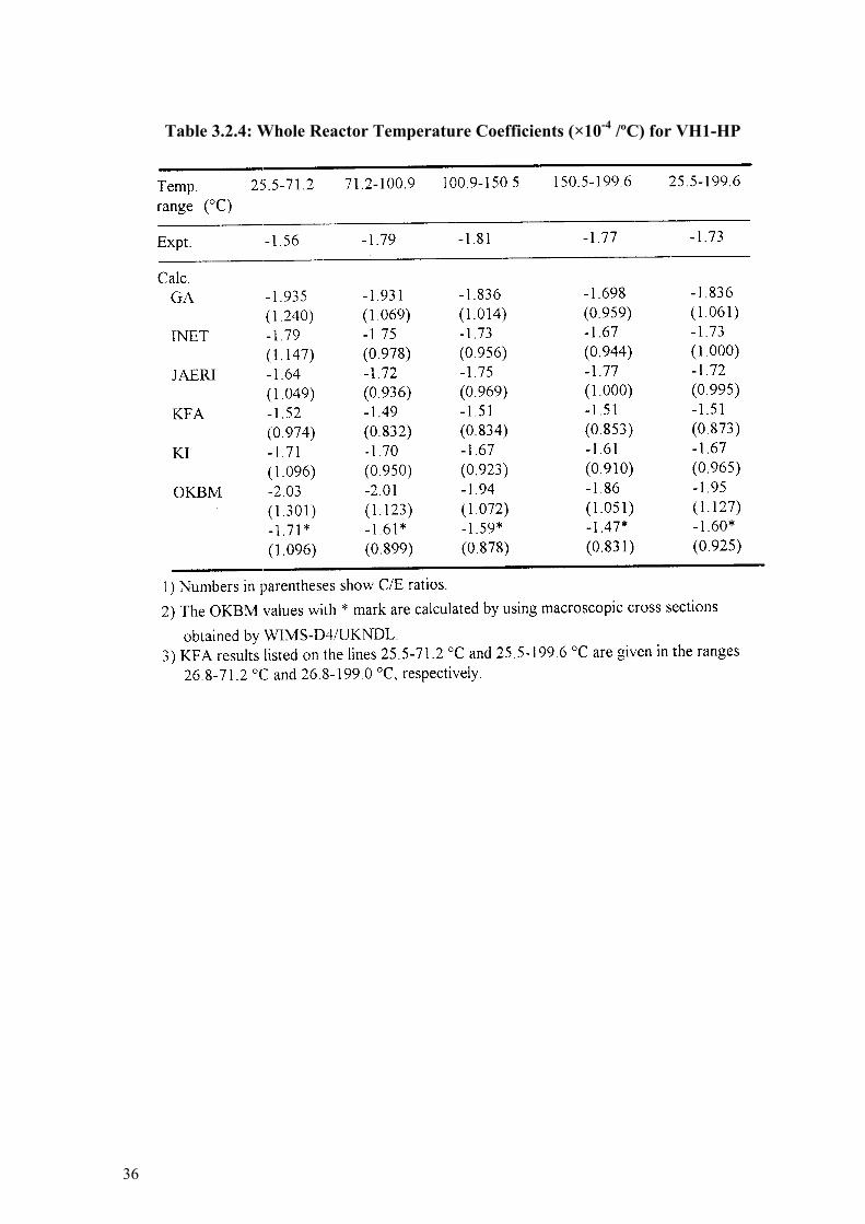
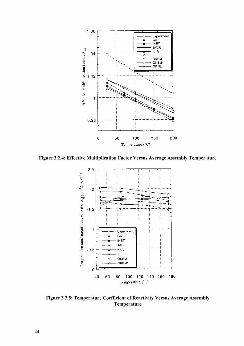
The values of the most important parameter, keff for the whole reactor, showed good agreement between all institutes, for both VH1-HP and VH1-HC and at all temperatures (see Figure 3.2.4 and Tables 3.2.2 and 3.2.3). They also agreed with the experimental values typically to within 1%, with all of the calculated values being higher than the experimental ones. As for the temperature coefficient of reactivity, all the calculated values of average (integral) temperature coefficient between room temperature and 200°C agreed with the experimental value to within 13% (see Figure 3.2.5 and Table 3.2.4). However, the calculated differential temperature coefficients showed varying degrees of temperature dependence in the analyzed temperature range, and these trends, which were not consistent with the experimental trend, could not be satisfactorily explained. This suggests that some uncertainty will remain in scaling the calculational accuracy to a higher temperature range.

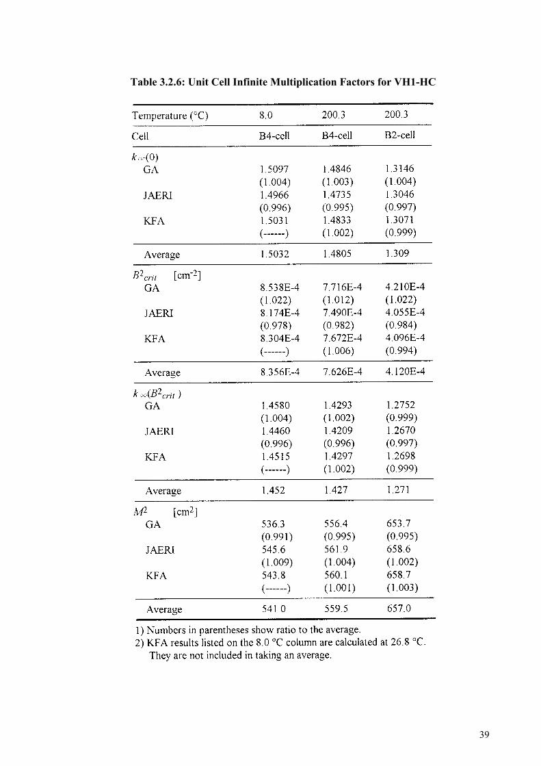
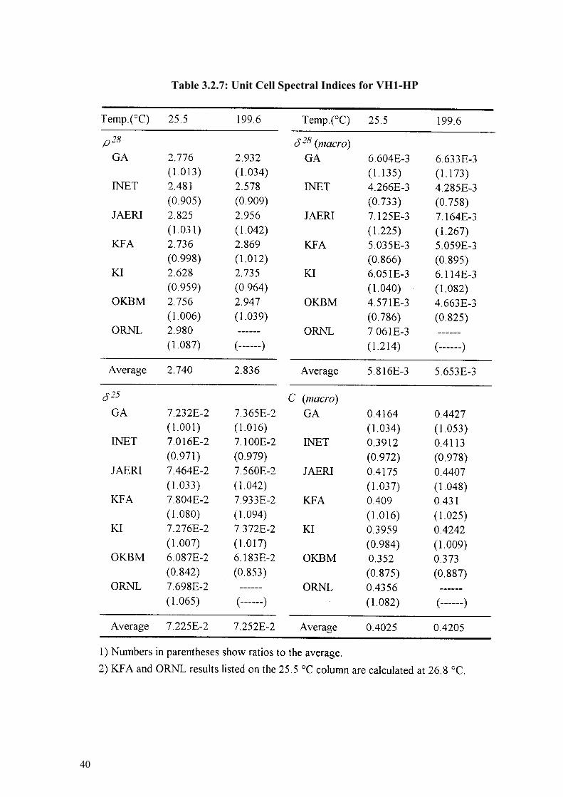
The values of several cell parameters calculated by some institutes did not agree very well with those from other institutes. Agreement in the values of the infinite multiplication factor, kinf, (see Tables 3.2.5 and 3.2.6) is much better than that for the spectral indices (see Tables 3.2.7 and 3.2.8). The δ 28 (fission ratio of 238U to 235U) values calculated by all institutes for instance showed considerable scatter. A similar tendency has been pointed out in the HTR-PROTEUS benchmark results.

Results for radial and axial fission rate distributions were provided by three institutes and showed discrepancies due mainly to the different geometrical models adopted in the whole reactor calculations (see Figure 3.2.6). The requested calculation item, effective delayed neutron fraction βeff , was not calculated except by JAERI and a comparison could therefore not be made. This item is important from a reactivity scale point of view and should be investigated in future work for a better understanding of HTR neutronics.

REFERENCES

[3.2.1] YASUDA, H., YAMANE, T., TSUCHIHASHI, K., “VHTRC Temperature Coefficient Benchmark Problem”, Presented at the Second RCM in Tokai, Japan on 20-22 May 1991.

[3.2.2] MATHEWS, D., CHAWLA, R., ”LEU-HTR PROTEUS Calculational Benchmark Specifications”, PSI Technical Memorandum TM-41-90-32 (9 Oct. 1990)

[3.2.3] YASUDA, H., YAMANE, T., SASA, T., “VHTRC Temperature Coefficient Benchmark Problem”, JAERI-Data/Code 94-013 (1994)

[3.2.4] YAMANE, T., et al., “Measurement of Overall Temperature Coefficient of Reactivity of VHTRC~1 Core by Pulsed Neutron Method”, J. Nucl. Sci. Technol., Vol. 27, No.2, (1990) p122

[3.2.5] YASUDA, H., et al.,: “Measurement of Temperature Coefficient of Reactivity of VHTRC-1 Core by Criticality Method”, Proc. IAEA Specialists Meeting on Uncertainties in Physics Calculations for Gas-Cooled Reactor Cores, Villigen, Switzerland, 9-11 May, 1990, IWGGCR/24 (1991).

[3.2.6] YASUDA, H., YAMANE, T., “Compilation Report of VHTRC Temperature Coefficient Benchmark Calculations”, JAERI-Research 95-081 (1995)

33

Table 3.2.1: Methods and Data used For the Calculation of the VHTRC Benchmark

Problem

34

Table 3.2.2: Whole Reactor Effective Multiplication Factors for VH1-HP

35

Table 3.2.3: Whole Reactor Effective Multiplication Factors for VH1-HC

36

Table 3.2.4: Whole Reactor Temperature Coefficients (×10-4

/ºC) for VH1-HP

37

Table 3.2.5: Unit Cell Infinite Multiplication Factors for VH1-HP

38

Table 3.2.5 (continued): Unit Cell Infinite Multiplication Factors for VH1-HP

39

Table 3.2.6: Unit Cell Infinite Multiplication Factors for VH1-HC

40

Table 3.2.7: Unit Cell Spectral Indices for VH1-HP

41

Table 3.2.8: Unit Cell Spectral Indices for VH1-HC at 200.3 °C

42

Figure 3.2.1: General Arrangement of the VHTRC Assembly

43

Figure 3.2.2: Core Loading Pattern for VH1-HP and the First Step of VH1-HC

Figure 3.2.3: Core Loading Pattern for the Second Step of Core VH1-HC

44

Figure 3.2.4: Effective Multiplication Factor Versus Average Assembly Temperature

Figure 3.2.5: Temperature Coefficient of Reactivity Versus Average Assembly

Temperature

45

Figure 3.2.6: Fission Distributions for VH1-HP, 25.5 °C, Calculated Using Effective

Cross Sections of the B-4 Unit Cell

46

4. PROTEUS CRITICAL EXPERIMENT FACILITY

The zero-power reactor facility PROTEUS is a part of the Paul Scherrer Institute (formerly EIR) and is situated near Würenlingen in the canton of Aargau in northern Switzerland

4.1. HISTORY OF THE FACILITY AND RECONFIGURATION FOR THE HTR EXPERIMENTS

PROTEUS has, in the past, been configured as a multi-zone (driven) system for the purpose of reactor physics investigations of both gas-cooled fast breeder and also high conversion reactors. For these experiments, the various test configurations were built into a central, sub-critical test-zone which was driven critical by means of annular, thermal driver-zones. For the LEU-HTR experiments described in this report however, PROTEUS was for the first time, configured as a single zone, pebble bed system surrounded radially and axially by a thick graphite reflector.

The rest of this chapter gives a brief history of the facility, including a description of the rebuild work undertaken for the HTR experiments, followed by a brief description of the present HTR-PROTEUS system.

• Jan. 1968 - Sep. 1970

Operation as a “zero-reactivity experiment” with a thermal, D2O moderated test-lattice and a graphite driver [4.1]

• Sep. 1970 - Apr. 1972

Mixed fast-thermal system with a “buffer-zone” and reduced size test-zone.

• Apr. 1972 - Apr. 1979

Sixteen different configurations of the gas-cooled fast reactor type [4.2].

• Jan. 1980 - Aug. 1980

Preliminary HTR experiments [4.3].

• Aug. 1980 - May 1981

Rebuild of the test-zone to accommodate light-water high conversion reactor experiments.

• May 1981 - Oct. 1982

Phase I of the advanced light-water reactor experiments. Six configurations were investigated [4.4].

• Feb. 1983 - May 1985

Re-configuration of the test-zone for Phase II of the light-water high conversion reactor experiments.

• Jun. 1985 - Dec. 1990

Phase II of the advanced light-water experiments - fourteen different test-zones, containing more representative fuel than in phase I, were investigated [4.5].

• Jan. 1991 - Jul. 1991

Rebuild for the LEU-HTR experiments. A brief summary of the work undertaken for this rebuild is now given:

47

♦ All driver and buffer fuel discharged and stored.

♦ Fuel in test-zone discharged and stored.

♦ All installations inside graphite-reflector removed.

♦ Construction of upper reflector assembly for HTR, an aluminum tank containing an annular region of old graphite and a central cylinder of new graphite.

♦ Filling of ~50% of the ~300 C-driver holes with new graphite rods. The other ~50% were filled with existing graphite rods.

♦ Renewal of the safety/shutdown rods - increased length to allow for greater core-height and better characterization of material properties - for improved benchmark quality of the experiments.

♦ Increased height of radial reflector by 12cms.

♦ Reconstruction of lower axial reflector, including central part of new graphite.

♦ Mounting of graphite panels in core cavity to modify the cavity shape to accommodate deterministic loadings.

♦ Fuel and moderator pebbles loaded.

♦ After the rest worths of the original ZEBRA control rods were found to be unacceptably high, these rods were replaced with conventional withdrawable control rods

The next section contains a brief description of the HTR-PROTEUS facility.

4.2. HTR-PROTEUS FACILITY DESCRIPTION

The description contained in this section serves only to give the reader a qualitative picture of the facility. Full details, for use in the benchmarking of codes and data, including atom densities, can be found elsewhere [4.6, 4.7] and are not included here for reasons of space. Schematic representations of the system presented in Figures 1 and 2.

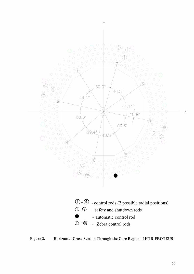
The HTR-PROTEUS system can be described as a cylinder of graphite, 3304mm in height and 3262mm in diameter. A central cavity, with base 780mm above the bottom of the lower axial reflector and having a horizontal cross-section in the form of a 22 sided polygon with a flat-to-flat separation of 1250mm, contains fuel (16.7% enriched) and moderator (pure graphite) pebbles, either randomly arranged or in one of several different geometrical arrangements. Additional graphite filler pieces are used at the core-reflector boundary to support the irregular outer surface of the deterministic pebble arrangements. A removable structure in the form of a graphite cylinder of height 780mm contained within an aluminum tank forms the upper axial reflector, normally with an air gap between it and the top of the pebble bed. An aluminum "safety ring", which is designed to prevent the upper axial reflector from falling onto the pebble-bed, in the case of an accident, is located some 1764mm above the floor of the cavity.

Shutdown of the reactor is achieved by means of 4 boron-steel rods situated at a radius of 680mm and reactor control by four fine control rods at a radius of 900mm. In Core 1 of the program, these fine control rods comprised Cd Shutter or ZEBRA type rods, but in all

48

subsequent cores, conventional, withdrawable stainless-steel rods were employed. A further, single servo-driven control rod, known as the autorod is also situated in the radial reflector. This rod is used to maintain the reactor in a critical state by responding to changes in the power level measured by a fixed ionization chamber.

For the simulation of water ingress, polyethylene rods are introduced to the vacant axial channels of the deterministic cores.

The system can be conveniently separated into the following groups of components:

• Fuel and moderator pebbles • Graphite - radial, upper and lower axial reflectors and filler pieces • Aluminum structures • Shutdown rods • Fine control rods • Automatic control rod • Static "Measurement Rods" • Polyethylene rods used to simulate water ingress • Miscellaneous components

Each of these component groups will now be described

4.2.1. Fuel, Moderator and Absorber Pebbles

Since the arrangement of fuel and moderator pebbles, by definition, changes from configuration to configuration, only the properties of the individual pebbles will be described in this section. Detailed descriptions of the pebble arrangements in each of the different core configurations are to be found in [4.7].

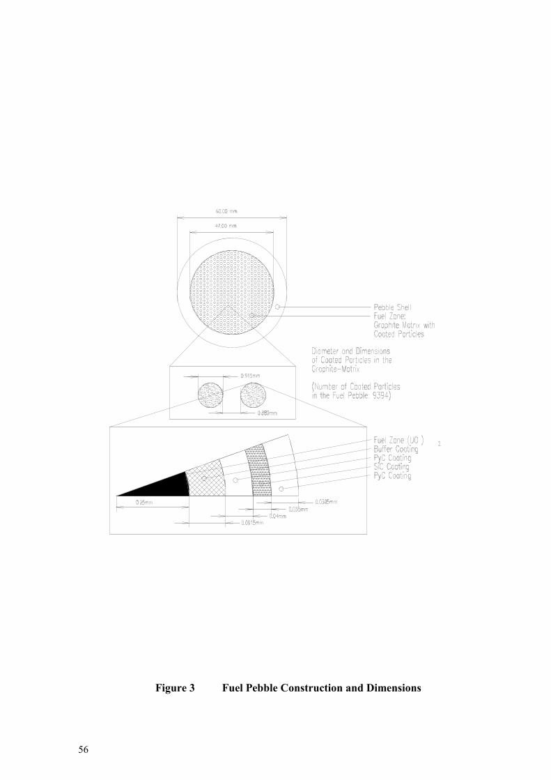
The main properties of the fuel pebbles are summarized in Table 1 and Figure 3. As a result of concerns that the manipulation of the pebbles during loading and unloading operations could have led to some erosion of the pebbles, the diameter and mass of the fuel pebbles was measured at PSI on 17.08.92 and again, after more than 3 years of experimentation, on 30.10.95. The masses of the fuel pebbles were not seen to have changed significantly over this period, although some slight reduction was observed in the average pebble diameter. This is presumed not to be due to a general loss of material from the fuel pebbles, but rather as a consequence of the diameter measurement technique in which the length of rows of 10 fuel pebbles were measured. The apparent diameter reduction was attributed to the presence of slight indentations in the surfaces caused during the loading process and is not thought to be significant. The measurements made on 17.08.92 appear in Table 1 and are those recommended in the system description [4.6]. As a by-product of these measurements it could be shown that fuel and moderator pebbles have nearly identical diameters, which was important for the geometric characterization of the regular pebble arrangements, containing different numbers of fuel and moderator pebbles.

The main properties of the moderator pebbles (obtained from measurements made at PSI on 17.8.92, 3.5.95 and 30.10.95) are given in Table 2. The values correspond well with those from the relevant QC records. No significant changes were noted in the properties of the moderator pebbles during the course of the experiments. The total boron equivalent of 1.39

49

millibarns given in the table results in an effective moderator pebble graphite 2200 m/s absorption cross section of 4.79 millibarns. Not included in the table are values for absorbed moisture in the pebbles. The amount of moisture contained in the pebbles was measured at PSI by choosing, at random, two moderator pebbles and heating them to 500°C in a vacuum for 5 hours. Each pebble showed a weight loss of 0.02g (0.01wt%).

4.2.2. Reflector Graphite Specifications

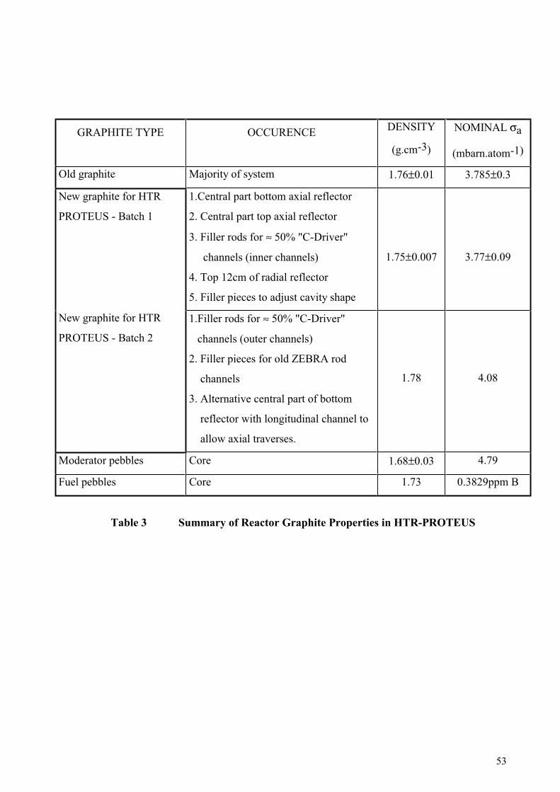
The HTR-PROTEUS reflector consists of graphite of various ages and from several different sources. The location of the various types of graphite is summarized in Table 3 along with the densities and nominal, "as delivered", impurity contents. It is seen in the table that the old graphite comprises the majority of the system, and therefore a global value of 1.763 g/cm3 is recommended for the graphite density.

No attempt is made to describe the impurity content of individual components. Instead, it is recommended that the global value, measured and reported in [4.8] be used as a universal impurity content, expressed in terms of equivalent boron content. This recommended value is 4.09±0.05 mbarn and it should be noted that this approach has the advantage that absorbed moisture and intergranular nitrogen (air) is automatically taken into account.

4.2.3. Upper Reflector Tank

This is a complex structure which supports the graphite of the upper reflector in place above the cavity. It comprises two main parts, an inner and an outer aluminum tank. The inner tank, which contains a cylinder of graphite 780mm high and 394mm in diameter, is removable and indeed must be removed before the main outer structure can be removed. This main outer structure contains an annulus of graphite having again a height of 780mm, an inner diameter of 418.6mm and an outer diameter of 1234mm.

4.2.4. Safety/Shutdown Rods

There are eight, identical, borated-steel safety/shutdown rods located adjacent to the core in the radial reflector. These eight rods are separated into two groups with four rods in each group (rods 1-4 and rods 5-8). One of these groups is selected as the "safety rod'' group and the other as the "shutdown rod' group. It should be remembered that the term "control rods" is reserved for the four, much lower reactivity worth, Zebra type Cd/Al reactivity control devices used in LEU-HTR PROTEUS Core 1 or the withdrawable stainless steel control rods used in Cores 1A onwards. The safety/shutdown rods consist of 35 mm diameter, borated steel rod-sections (nominally 5 wt% boron) enclosed in 18/8 stainless steel tubes of outside diameter 40mm and inside diameter 36mm. The rods are located in 45mm inner diameter graphite guide tubes in the radial reflector. The centers of the 45mm inner diameter guide tubes are 684 mm from the center of the core or about 59mm from the inner surface of the radial reflector (without filler pieces). The azimuthal positions of the 8 rods are shown in Figure 2 in which the slight azimuthal asymmetry of the rod positions should be noted.

4.2.5. Zebra Type Cd/Al Control Rods

Four Cd/Al control rods of the "Zebra'' type were used in LEU-HTR PROTEUS Core 1. This type of control rod has the advantage that it causes minimal perturbations to the axial flux

50

distribution at the price of a significant minimum (rest) reactivity worth. Because the minimum reactivity worth of this type of control rod varies with the core configuration and is somewhat time consuming to determine experimentally, the Zebra type control rods were used only in Core 1 and were then replaced by standard withdrawable type stainless-steel control rods.

4.2.6. Withdrawable Stainless Steel Control Rods

The control rods which replaced the ZEBRA rods described in the last section and which were used in all cores from 1A onwards are of the conventional withdrawable type. The rods are not situated in the same channels as the ZEBRA rods but rather in 4 C-Driver channels. With the intent of increasing operational flexibility, the new rods were designed to be operable at two radii, namely 789mm (ring 3) or 906mm (ring 5). Due to the thermal flux gradient in the radial reflector at these positions, significantly different rod worths are thus achievable. Figure 2 indicates the control-rod positions.

4.2.7. Automatic Control Rod

This is a single fine control rod, situated in the radial reflector at a radius of ~ 900mm and used to automatically maintain the critical reactor at a nominal demanded power. It responds to the signal from a single ionization chamber also situated in the radial reflector. The rod itself comprises a wedge shaped copper plate supported within an aluminum tube.

4.2.8. Static Measurement Rods

In order to investigate the spatial dependence of control-rod worths in a particular configuration and because the operational control rods are restricted in their locational possibilities, simulated control rods were specially manufactured for the experiments. These rods are so designed that they may be inserted either into the C-Driver channels in the radial reflector or into a specially designed graphite sleeve which replaces a column of pebbles in a columnar hexagonal core. Because the core and radial reflectors are of significantly different heights, it was necessary to produce two pairs of rods, which apart from their axial dimensions are nominally identical.

4.2.9. Polyethylene Rods

One of the main aims of the HTR PROTEUS project was the measurement of the effect of accidental water ingress to the core. Because the use of water in the experiments was 1) forbidden and 2) impractical, the presence of moisture was simulated by means of polyethylene rods. In order to simulate a range of water densities in the void space between the pebbles of the different geometrical configurations, a number of different shapes and sizes of polyethylene rods were used. The dimensions and specific densities, of the available rods are detailed in Figure 4. Most of the rods were produced in two variations, machined and unmachined. It was envisaged that the, cheaper, unmachined rods, which were expected to be less homogeneous along their length, would be used for approaches to critical, with the much more expensive, machined rods being used for the final critical balance, since these were (in theory) better characterized. However, measurements at PSI have subsequently shown that the 6 and 9mm unmachined rods show, surprisingly, a somewhat higher homogeneity than the

51

machined versions, with the added advantage that the unmachined rods have not been exposed to an extra ‘impurity hazardous’ machine environment.

4.2.10. Miscellaneous

In at least one configuration (Core 6), an attempt was made to compensate the positive reactivity effect of adding polyethylene to the core by simultaneously adding high purity copper wire to the core region. The copper wire used was 99.9% pure and had a nominal diameter of 1.784mm and a specific density of 0.2232g/cm.

REFERENCES

[4.1] H.R. LUTZ et al., “Slightly Enriched Uranium Single -Rod Heavy - Water Lattice Studies“, EIR Bericht No. 99, September 1966.

[4.2] R. RICHMOND, “Measurement of the Physics Properties of Gas-Cooled Fast Reactors in the Zero Energy Reactor PROTEUS and Analysis of the Results“, EIR Report No. 478, December 1982

[4.3] R. RICHMOND and J. STEPANEK, “Application of a Coupled Zero Energy Reactor for Physics Studies of HTR Systems“, EIR Internal Report TM-22-81-25, August 1981

[4.4] R. CHAWLA et al., “Reactivity and Reaction-rate Ratio Changes with Moderator Voidage in a Light Water High Converter Reactor Lattice“, Nucl. Technol, 67,360(1984).

[4.5] H.-D. BERGER et al., “Dokumentation der PROTEUS-FDWR Phase II-Experimente“, PSI Internal Report TM-41-93-05, May 1993

[4.6] D. MATHEWS and T. WILLIAMS, "LEU-HTR PROTEUS System Component Description", PSI Internal Report TM-41-93-43, November 1995.

[4.7] T. WILLIAMS, "Configuration Descriptions and Critical Balances for Cores 1-7 of the HTR-PROTEUS Experimental Programme", PSI Internal Report TM-41-95-18, November 1995.

[4.8] T. WILLIAMS, "Measurement of the Absorption Properties of the HTR-PROTEUS Reflector Graphite by Means of a Pulsed-Neutron Technique", PSI Internal Report TM-41-93-34, October 1995.

52

Tables

235U mass per fuel pebble 1.000±0.01g

238U mass per fuel pebble 4.953±0.05g

Total U mass per fuel pebble 5.966±0.06g

Carbon mass per fuel pebble 193.1±0.2g

Total mass per fuel pebble 202.22±0.18g

Fuel pebble inner (fueled) zone radius 2.35±0.025cm

Fuel pebble outer radius 3.0006±0.002cm

Radius of fuel particles (UO2) 0.0251±0.001cm

Density of fuel particles 10.88±0.04g/cm3

Table 1. LEU-HTR Fuel Pebble Physical Specifications

Moderator pebble mass 190.54±1.44g

Moderator pebble outer radius 2.9979±0.0015cm

Table 2 Moderator Pebble Specifications

53

GRAPHITE TYPE OCCURENCE DENSITY

(g.cm-3)

NOMINAL σa

(mbarn.atom-1)

Old graphite Majority of system 1.76±0.01 3.785±0.3

New graphite for HTR

PROTEUS - Batch 1

1.Central part bottom axial reflector

2. Central part top axial reflector

3. Filler rods for ≈ 50% "C-Driver"

channels (inner channels)

4. Top 12cm of radial reflector

5. Filler pieces to adjust cavity shape

1.75±0.007 3.77±0.09

New graphite for HTR

PROTEUS - Batch 2

1.Filler rods for ≈ 50% "C-Driver"

channels (outer channels)

2. Filler pieces for old ZEBRA rod

channels

3. Alternative central part of bottom

reflector with longitudinal channel to

allow axial traverses.

1.78 4.08

Moderator pebbles Core 1.68±0.03 4.79

Fuel pebbles Core 1.73 0.3829ppm B

Table 3 Summary of Reactor Graphite Properties in HTR-PROTEUS

54

Figures

Figure 1. A Schematic Side View of the HTR-PROTEUS Facility (dimensions in mm)

55

�-� - control rods (2 possible radial positions)

�-� - safety and shutdown rods

� - automatic control rod

- Zebra control rods

Figure 2. Horizontal Cross-Section Through the Core Region of HTR-PROTEUS

I IV-

56

Figure 3 Fuel Pebble Construction and Dimensions

57

2.96mm diameter 0.0667±0.00006g/cm

(machined)

3mm diameter 0.06616±0.00006g/cm(unmachined)

5.9mm diameter 0.2575±0.0001g/cm(machined)

6.5mm diameter 0.3161±0.0001g/cm(un-machined)

8.3mm diameter 0.5087±0.0007g/cm(un-machined)

8.9mm diameter 0.5867±0.0019g/cm(machined)

13.5mm sides 0.646±0.05g/cm6mm hole

25mm diameter 4.808±0.001g/cm

Figure 4 Physical Properties of the Available Polyethylene Rods

58

5. PROTEUS EXPERIMENT PLANS

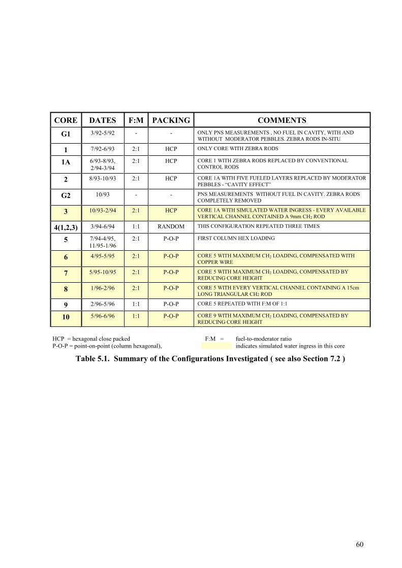
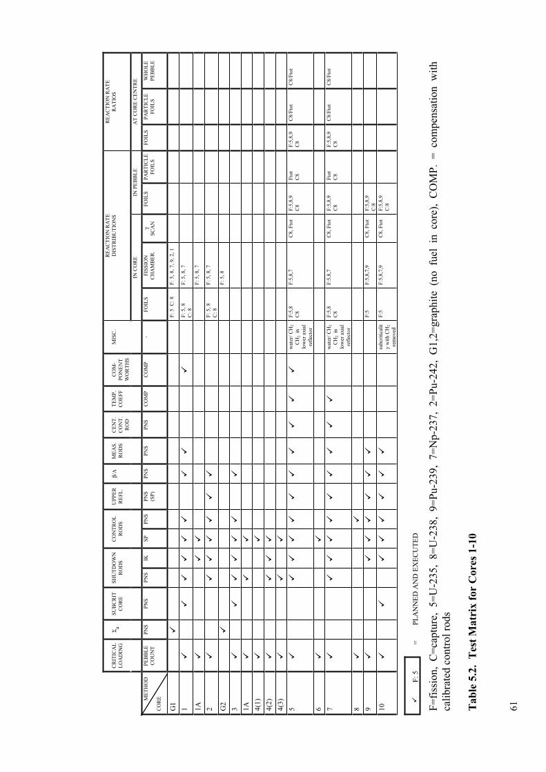
This chapter contains descriptions of the experiments carried out on each of the ten different HTR-PROTEUS configurations. The information is provided in table form for ease of reference. Table 5.1. contains a brief description of each of the configurations; this table is only intended for orientation purposes, more detailed descriptions are to be found in Section 7.2. The time periods spanned by each of the configurations is also given in Table 5.1. and represented graphically in Figure 5.1. In Table 5.2. a summary of the parameters investigated in each of these configurations is presented in the form of a “test matrix”. An explanation of the experiment identifiers appearing in Table 5.2 is provided below for each parameter, with reference being made to the detailed descriptions of the measurement techniques given in Section 6.

Since each configuration was planned with the investigation of one or more particular physics aspects in mind, the type of parameters measured varies considerably from core to core. A summary of the measurements made in each core is provided in Table 5.2 and brief details of each of the measurements referred to in the table is given below. Further details can be found in Section 6 of this report

Critical Loading

The measurement of the critical height of the core and/or the number of fuel and moderator pebbles loaded. Every effort was made to obtain critical configurations which were as clean as possible, especially with respect to control rod insertions, presence of start-up sources, temperature instrumentation etc. Operationally speaking, these critical loadings are not usually very convenient; for instance a low control-rod insertion implies a very small excess reactivity and often leads to problems during power raising. Therefore, the critical loadings quoted in the results section are often not the final operational states for that core.

The loading procedure is described in detail in section 6.1. This is arguably the most important parameter and was therefore recorded for every configuration.

ΣΣΣΣa

The measurement of the absorption cross section of the reactor graphite using PNS techniques. Although this parameter is not one of those required from the program, a knowledge of its magnitude is imperative for the accurate definition of the PROTEUS facility, see Sections 6.5. and 4.2.

Subcritical Core

The use of the PNS technique to measure a subcritical state. For instance in Core 1 a measurement of the subcriticality of the system was made with 16 layers loaded. Details of the PNS technique are given in Section 6.2.1.

Shutdown rods

The measurement of the integral worth of 1, 2, 3, 4 or 8 bulk absorber rods using either PNS (Section 6.2.1.) or IK (see Section 6.2.2). In Section 4 it was explained that there are eight bulk absorber rods and that four can be selected as safety and four as shutdown. Because the system interlocks only allow individual insertion of the shutdown rods, these rods were always selected as the ones to be measured. Various rod configurations were measured in order to investigate rod interaction effects.

59

Control rods

The measurement of the integral and differential worth of the individual control rods using the stable period technique (see Section 6.2.1.1.2.). Combinations of rods were not measured as interference effects have been seen to be small [5.1]. The accurate calibration of these rods in every core was very important as the rods are used to establish a critical balance and thus are needed to estimate the reactivity excess.

Upper reflector

The measurement of the worth of the upper reflector assembly by means of its removal and subsequent PNS measurement (see Section 6.2.1.)

ββββ/ΛΛΛΛMeasurement of the kinetic parameter, β/Λ, at critical. This parameter is of particular interest to the Japanese who observe significant C/E discrepancies in VHTRC. Full details of this measurement are given in Section 6.4.

Measurement rod

Measurement of the reactivity worth of specially designed dummy control rods which can be placed in channels in the radial reflector. The rods consist of aluminum tubes containing pellets of boron-steel (see Section 4.2. for specifications). Used to investigate radial dependence of control rod worth. PNS technique used (see Section 6.2.1.)

Central control Rod

Similar to the above measurement. By means of a graphite sleeve in place of a column of pebbles, the worth of a dummy control rod in the core center is measured using the PNS technique (see 6.2.1.). This measurement can only be carried out in point-on-point cores.

Temperature Coefficient of Reactivity

The measurement of the temperature coefficient of reactivity around room temperature by means of controlling system temperature with the air conditioning system. It is only possible to produce temperature effects of around ±10°C. Effect is measured using calibrated control and auto rods

Component Worths

The measurement of the reactivity worth of the various components which represent perturbations to the clean system. Effect measured using calibrated control and autorods.

Reaction rate distributions

In core The measurement of core axial and radial reaction-rate distributions between the pebbles using activation foils and miniature fission chambers or the measurement of core axial and radial reaction-rate distributions using γ-scanning of irradiated fuel pebbles (see 6.3.1.)In pebble The measurement of reaction rate distributions within the pebbles themselves using conventional foils or special fuel particle foils (see 6.3.1.)

Reaction rates and ratios

The measurement of core-center reaction-rates and ratios within the pebbles themselves using conventional activation foils and graphite foils containing fuel particles (see section 6.3.2.)

60

CORE DATES F:M PACKING COMMENTS

G1 3/92-5/92 - - ONLY PNS MEASUREMENTS , NO FUEL IN CAVITY, WITH AND WITHOUT MODERATOR PEBBLES. ZEBRA RODS IN-SITU

1 7/92-6/93 2:1 HCP ONLY CORE WITH ZEBRA RODS

1A 6/93-8/93, 2/94-3/94

2:1 HCP CORE 1 WITH ZEBRA RODS REPLACED BY CONVENTIONAL CONTROL RODS

2 8/93-10/93 2:1 HCP CORE 1A WITH FIVE FUELED LAYERS REPLACED BY MODERATOR PEBBLES - “CAVITY EFFECT”

G2 10/93 - - PNS MEASUREMENTS WITHOUT FUEL IN CAVITY. ZEBRA RODS COMPLETELY REMOVED

3 10/93-2/94 2:1 HCP CORE 1A WITH SIMULATED WATER INGRESS - EVERY AVAILABLE VERTICAL CHANNEL CONTAINED A 9mm CH2 ROD

4(1,2,3) 3/94-6/94 1:1 RANDOM THIS CONFIGURATION REPEATED THREE TIMES

5 7/94-4/95, 11/95-1/96

2:1 P-O-P FIRST COLUMN HEX LOADING

6 4/95-5/95 2:1 P-O-P CORE 5 WITH MAXIMUM CH2 LOADING, COMPENSATED WITH COPPER WIRE

7 5/95-10/95 2:1 P-O-P CORE 5 WITH MAXIMUM CH2 LOADING, COMPENSATED BY REDUCING CORE HEIGHT

8 1/96-2/96 2:1 P-O-P CORE 5 WITH EVERY VERTICAL CHANNEL CONTAINING A 15cm LONG TRIANGULAR CH2 ROD

9 2/96-5/96 1:1 P-O-P CORE 5 REPEATED WITH F:M OF 1:1

10 5/96-6/96 1:1 P-O-P CORE 9 WITH MAXIMUM CH2 LOADING, COMPENSATED BY REDUCING CORE HEIGHT

HCP = hexagonal close packed F:M = fuel-to-moderator ratio P-O-P = point-on-point (column hexagonal), indicates simulated water ingress in this core

Table 5.1. Summary of the Configurations Investigated ( see also Section 7.2 )

61

CR

ITIC

AL

L

OA

DIN

G

Σ aS

UB

CR

IT

CO

RE

S

HU

TD

OW

N

RO

DS

C

ON

TR

OL

R

OD

S

UP

PE

R

RE

FL

. β/

ΛM

EA

S.

RO

DS

C

EN

T.

CO

NT

. R

OD

TE

MP

. C

OE

FF

C

OM

-P

ON

EN

T

WO

RT

HS

MIS

C.

RE

AC

TIO

N R

AT

E

DIS

TR

IBU

TIO

NS

R

EA

CT

ION

RA

TE

R

AT

IOS

IN

CO

RE

IN

PE

BB

LE

A

T C

OR

E C

EN

TR

E

ME

TH

OD

CO

RE

PE

BB

LE

C

OU

NT

P

NS

P

NS

P

NS

IK

S

P

PN

S

PN

S

(SP

)P

NS

P

NS

P

NS

C

OM

P

CO

MP

-

FO

ILS

F

ISS

ION

C

HA

MB

ER

. γ

SC

AN

F

OIL

S

PA

RT

ICL

E

FO

ILS

F

OIL

S

PA

RT

ICL

E

FO

ILS

W

HO

LE

P

EB

BL

E

G1

�

F

: 5

C:

8 F

: 5,

8, 7

, 9, 2

, 1

1�

��

��

��

��

F

: 5,

8

C:

8 F

: 5,

8, 7

1A

�

��

F

: 5,

8, 7

2�

��

��

��

F

: 5,

8

C:

8 F

: 5,

8, 7

G2

�

F:

5, 8

3�

��

��

��

1A

��

�

4(1)

�

�

4(2)

�

��

�

4(3)

�

��

5�

��

��

��

��

��

wat

er/

CH

2

CH

2 in

lo

wer

axi

al

refl

ecto

r

F:5

,8

C8

F:5

,8,7

C

8, F

tot

F:5

,8,9

C

8 F

tot

C8

F:5

,8,9

C

8 C

8/F

tot

C8/

Fto

t

6�

�

7�

��

��

��

��

�w

ater

/ C

H2

CH

2 in

lo

wer

axi

al

refl

ecto

r

F:5

,8

C8

F:5

,8,7

C

8, F

tot

F:5

,8,9

C

8 F

tot

C8

F:5

,8,9

C

8 C

8/F

tot

C8/

Fto

t

8�

�

9�

�

��

��

�

F

:5

F:5

,8,7

,9

C8,

Fto

t F

:5,8

,9

C:8

10�

��

��

��

�

subc

riti

calit

y w

ith

CH

2

rem

oved

F:5

F

:5,8

,7,9

C

8, F

tot

F:5

,8,9

C

:8

�F

: 5

=

PL

AN

NE

D A

ND

EX

EC

UT

ED

F=

fiss

ion,

C=

capt

ure,

5=

U-2

35,

8=U

-238

, 9=

Pu-

239,

7=

Np-

237,

2=

Pu-

242,

G1,

2=gr

aphi

te (

no f

uel

in c

ore)

, C

OM

P.

= c

ompe

nsat

ion

wit

hca

libr

ated

con

trol

rod

s

Tab

le 5

.2.

Tes

t M

atr

ix f

or

Core

s 1-1

0

62

ANALYSIS

CORE 10

CORE 9

CORE 8

CORE 5

CORE 7

CORE 6

CORE 5

CORES 4(1,2,3)

CORE 1A

CORE 3

G2

CORE 2

CORE 1A

CORE 1

PLANNING

CRP

Jan 90 Jan 91 Jan 92 Jan 93 Jan 94 Jan 95 Jan 96

ANALYSIS

CORE 10

CORE 9

CORE 8

CORE 5

CORE 7

CORE 6

CORE 5

CORES 4(1,2,3)

CORE 1A

CORE 3

G2

CORE 2

CORE 1A

CORE 1

PLANNING

CRP

Figure 5.1 Time Allocation to Each of the HTR PROTEUS Configurations

63

6. PROTEUS MEASUREMENT TECHNIQUES

For the purposes of this report, the HTR-PROTEUS experimental methodologies have been described under five headings:

1. Critical loadings 2. Reactivity 3. Kinetic parameter 4. Reaction-rates 5. Absorption cross-section of the reactor graphite

These categories do not differentiate between individual measurement techniques as such, but rather between the experimental determination of different parameters, each of which may involve the use of several different individual measurement techniques. Furthermore, the same measurement technique may appear under more than one heading, e.g. the Pulsed Neutron Source measurement technique appears in three of the five categories.

The descriptions which follow include the theoretical basis, the practical application and the analysis strategy of each method. It is not intended to present an exhaustive description of each technique. The interested reader is invited to refer to the large number of technical reference documents for further details of the experiments. In particular, the three doctoral theses of Rosselet, Wallerbos and Köberl [6.1, 6.2, 6.3] present in sufficient detail the experimental techniques used for the reactivity, kinetic parameter and reaction rate measurements. Last, but by no means least, it should be mentioned that, during the course of the programme, a great deal of experimental development work has been carried out, which has to a great extent, solved the problems associated with measurements in such systems. Although the results of techniques developed are presented in chapters 7 and 8 of this work, the details of the experimental developments are well outside the scope of the present document. In depth descriptions however can be found in the various documents referred to in this chapter.

6.1. CRITICAL LOADINGS

The “approach-to-critical” for each configuration was accompanied by the usual inverse

counts versus core loading plot with an extrapolation to 1/counts = 0 being made after each pebble loading step to give the predicted critical loading (see for example reference [6.4]). After the first two loading steps, which were administratively limited to 1/3 and 1/6 of the number of pebbles predicted for the critical loading respectively, the remaining steps were limited [6.5] to one half of the predicted additional number of pebbles required to achieve criticality or the worth of the control rod bank, whichever was the larger. The count rates were measured using neutron detectors situated in the radial reflector. Because the loading of a pebble bed involves a continuous core height and thus core-detector geometry change, it was expected that the approach curves would show considerable spatial dependence and for this reason, early loadings were monitored with additional detectors. The approach curves showed considerable non-linearity for detectors close to the core, with a noticeable effect as the core upper surface reached the axial position of the detector. For this reason, all subsequent approaches were made with detectors situated further out in the radial reflector. A full account of a typical approach is given in [6.4].

Criticality is established and power is raised by means of movements of the control rods. Criticality is maintained by means of the autorod, which is a single, radial-reflector-based rod

64

driven automatically by the signal from a “deviation channel”, to maintain reactor power and thus criticality. Since the deviation channel comprises an ionization chamber situated in the radial reflector, the signal noise and hence the accuracy of the determination of a critical configuration is determined by the flux level in the reactor. However, the autorod itself has typically a total worth of less than 0.1$ and the uncertainty in its position represents much less than ±5% of this range, even at relatively low fluxes. Such an uncertainty of <±0.005$ is regarded as negligible.

Although the HTR-PROTEUS system is a reasonably clean one, some correction to the critical state must be made for excess reactivity due to effects such as control rod/autorod insertion at critical, reactor instrumentation in the system etc. To this end, the individual, differential control-rod worths were measured in every configuration and the magnitude of all other effects estimated by means of the compensation technique using these calibrated rods (see for example [6.6]). For reasons of time, these component worths were only measured in selected cores and the values for all other intermediate configurations inferred from the differences between control rod bank worths. These corrections to the actual critical loading to yield the clean-critical loadings are given for each configuration in Section 7.2.

As described in Section 4.2, the various PROTEUS configurations comprised both random and deterministic (hexagonal close-packed and columnar hexagonal) loadings of pebbles, both of which require some careful consideration with regard to the establishment and definition of a critical loading.

6.1.1. Random

Fuel and moderator pebbles, in the desired ratio, were introduced to the cavity in a stepwise manner from a height above the core of about two meters (in order to encourage a truly random arrangement of pebbles). The loading process was carried out automatically with the aid of a pneumatic fueling machine, which was developed specially for the purpose and helped to considerably reduce operator doses during loading and unloading of the various configurations. Since the fuel and moderator pebbles are stored and delivered to the core separately, the first random loading (Core 4.1) was made by simply clamping the fuel and moderator pebble delivery tubes together in parallel and allowing each pebble to fall under gravity into the core from its respective tube. However, it was feared that this may lead to some unwanted ordering effects and indeed a visual inspection during loading suggested some asymmetry (the fuel and moderator pebbles could be differentiated by different surface finishes and by means of a ring inscribed on the fuel pebbles). Consequently, in all subsequent loading operations, the fuel and moderator channels were combined, by means of a simple, funnel-type arrangement, to alleviate this problem.

Having achieved a critical loading, the definitive measured parameter is the number of fuel and moderator pebbles loaded. In the deterministic cores, pebble accounting is simplified by virtue of the fact that it is well known how many fuel and moderator pebbles should reside in each layer and this can be compared, following the loading of each layer, with the number of pebbles registered as having left the fueling machine. In the random cores however this additional check is not possible and, as an additional precaution, having achieved criticality the number of pebbles remaining in the respective storage containers is compared with the expected value.

65

For random cores, the configuration is not fully defined until the core height and thus the core packing density is also determined. The packing fraction will not necessarily be equal to the theoretical random packing fraction of 0.62 [6.7] due to the presumably significant boundary (ordering) effects in the relatively small cavity. Special core cavity floor inserts were used for the random configurations to reduce such ordering effects. In the particular case of the random configurations, the determination of the core height is not straightforward and introduces a significant uncertainty to the definition of the system state. After a critical state had been achieved, the upper surface of the pebble bed was gently ‘flattened’ to achieve an optically even upper surface without compacting the pebble-bed. The average height of the top of the pebble bed was then determined in several radial directions. It was considered necessary to attribute an uncertainty of some 3cm (half a pebble diameter) to this value. The core heights and associated core packing fractions are summarized in Section 7.2.

6.1.2. Deterministic

The deterministic configurations were loaded by hand. Although the fueling machine was used to deliver pebbles to the loading personnel, each pebble had to be located effectively by hand. In order to facilitate access to the pebble bed, a specially constructed, shielded, “loading-basket” was used. The loading of the hexagonal close packed lattices was relatively simple, since the pebbles located themselves readily in the depressions between the pebbles in the layer below. The loading of the point-on-point cores however, presented more problems; namely in the support of half-finished layers. To this end, special anodized aluminum “tripods” were constructed, which could be removed once the layer was complete. The success of these simple devices represented a major benefit to the project as a whole, since a great deal depended upon the successful and efficient loading of point-on-point cores.

Although the deterministic loadings are significantly more time consuming to load, they possess several distinct advantages compared with the random loadings, including reproducibility and experimental access to the core center. One disadvantage however is that, as a result of the layered nature of these configurations and the fact that the worth of the top layer is often significantly larger than the control rod bank, it is not guaranteed that a satisfactory critical state will be achieved with a complete upper layer of pebbles. In the case of the hexagonal close packed lattice, this represents only a calculational inconvenience and a reduction in the “cleanness” of the calculational model, but in the case of the columnar hexagonal configurations it is somewhat more problematic since it is impossible, in this configuration, to load a partial layer of pebbles. For this reason, it has been necessary in some cores to load mixed final layers consisting of central fuelled regions and outer, pure moderator regions. As a final point it should be noted that, due to the fact that the worth of a pebble varies radially across the core, it is not sufficient in such cases to specify the number of pebbles in a deterministic loading - the precise geometry of the upper layer must also be specified.

6.2. REACTIVITY MEASUREMENTS

As stated in Section 2.4, accurate measurements of the reactivity worth of control absorbers in the core and reflector of configurations with a range of moderation properties was a very important aspect of the HTR-PROTEUS experimental program. Since HTR-PROTEUS was the first series of PROTEUS configurations which were self-critical (as opposed to driven) systems, there was little detailed experience in absolute reactivity measurements. Therefore, during the planning phase of the experiments, an extensive survey of all the commonly used

66

techniques was made, in order to assess the potential of the various methods and ultimately to decide which ones would be used for the experiments. The criteria on which this decision was made were as follows:

• the method must be compatible with small, highly reflected thermal systems • the method must be applicable to deeply subcritical cores • there must be as little dependence upon calculation as possible • the accuracy of the method should be greater than the current physics

methods for LEU HTRs • the methods chosen should be complimentary techniques, which are, as far as

possible, subject to different systematic errors or uncertainties [6.8] • the economics of the method should be justifiable.

The methods considered comprised subcritical source multiplication, inverse kinetics, reactor noise and pulsed neutron source.

In connection with this preliminary work, IAEA supported visits were made, by a member of the PROTEUS team, both to the VHTRC facility at JAERI to gain “hands-on” experience of pulsed neutron techniques and to KFA Jülich where discussions were undertaken with scientists who had worked on the critical experiments on KAHTER. The conclusions of these discussions are summarized in [6.9]

Ultimately it was decided, on the grounds of applicability, complimentarity and required effort, that the Pulsed Neutron Source (PNS) and Inverse Kinetics (IK) techniques would be the main “in-house” reactivity measurement techniques applied to HTR-PROTEUS. Furthermore, it was concluded that neutron noise measurements, although of some academic interest, would not be applied; as a result of the known difficulty of application to slow (long prompt generation time) systems and the large anticipated development effort required. In addition, noise measurements were not regarded as being complimentary to the inhour variation of the PNS technique (see later), since both methods are based upon the isolation of the prompt decay constant and the use of a calculated generation time to yield a value of reactivity in dollars (as it happens, a series of noise measurements were made by a visiting guest scientist, the results of this work being found in the thesis of Wallerbos [6.2]). The results of IK analysis, on the other hand, are very insensitive to estimates of the generation time and furthermore IK is regarded as a dynamic technique (e.g. rod drop from an initially critical state) whereas both noise and PNS are static techniques, which can be applied directly to a subcritical configuration without reference to a critical state.

What will be described below is the classical theory of pulsed neutron and inverse kinetic analysis. During the latter part of the HTR PROTEUS experimental programme, the classical methods were developed and applied in new ways to try and avoid the use of large correction factors. These developments, which are described in detail in [6.1], [6.10], [6.11] contributed significantly to improving the accuracy of the reported measurements and these measurements are reported in sections 7 and 8. A description of the new techniques which above all are based upon the use of epithermal detection systems is beyond the scope of the present work

6.2.1. Pulsed Neutron Source Measurements

Preliminary investigations of the applicability of PNS techniques to subcriticality measurements in HTR-PROTEUS were reported in [6.9, 6.12].

67

6.2.1.1. Theory

The possibility of using pulsed neutron sources to measure subcriticality was first suggested in the 1950’s by Sjöstrand [6.13] and by Simmons and King [6.14]. During the 1960’s and early 1970’s a great deal of work was carried out on improvements to- and applications of these basic techniques [6.15-6.19] but, in principle, all the techniques fall into one of the two categories - area-ratio or inhour. The theory of each of these two methods and the specific application of each of the techniques to HTR-PROTEUS will now be summarized:

6.2.1.1.1. Inhour Method

The theory of this method is described in [6.14, 6.12] and is discussed, in some detail, in [6.20].

The theory is based, as the name suggests, upon the well-known inhour equation, which is a single energy-group, quasi time-dependent representation of a point reactor system (for a derivation see [6.21, 6.20]). The inhour equation can be written as

ρ αβ

αα λ

($) = ++=

�Λ

eff

i

ii

n b

1

(6.1)

in which:

ρ

αλ

β

($) is the reactivity in units of dollars

is the prompt neutron generation time

is the number of delayed neutron groups

are the solutions, or roots, of the inhour equation ( in this work)

is the decay constant for the th delayed neutron group

is the fraction of delayed neutrons in the th group (normalised such that b )

is the total effective delayed neutron fraction

ii=1

n

Λn

n n

i

b i

i

i

eff

+ =

=�

1 6

1

For a subcritical system, all n + 1 values of α are negative and one, the most negative, is known as the prompt decay constant (α 0 ). The prompt decay constant depends strongly upon

the reactivity of the system whereas the other n values are bounded by the decay constants of the delayed neutron precursors and depend only weakly upon reactivity. The basis of the inhour analysis of PNS measurements is to isolate the single exponential α 0 from the delayed

background and to use this, with a knowledge of λ βi i effb, , and Λ , to derive a value of the

reactivity in dollars via equation (6.1). One of the main advantages of this technique is that the αs are global parameters of the system and do not depend greatly on experimental conditions, such as detector position.

In systems with relatively short generation times (e.g. light water reactors) α 0 is found to be

>> λ i and the following approximation is true:

ρ αβ

($) ≅ +Λ

eff

1 (6.2)

In slow, graphite moderated systems such as HTR-PROTEUS however, α 0 is similar in

magnitude to the most negative value of λ i , (-3.87 for 235U) especially when close to critical,

68

and the approximation in (6.2) is not valid (this corresponds to a situation in which the prompt decay in Figure 6.5 merges into the delayed background). It is still true to say, however, that the dependence of the derived value of ρ($) on the second term in equation (6.1) is a second

order one and that the most important parameter required to convert α 0 into ρ($) is the

reduced generation time Λ Λ* ( / )≡ β eff . Now, early studies [6.9] assumed the invariance of

Λ* with ρ($) such that:

ρ α αα

($) = − c (6.3)

in which αc is the value of α at critical (the subscript 0 has now been dropped but unless otherwise stated is implied)

However, for most applications of the technique, it is unacceptable to assume the invariability

of Λ* . On the other hand, if a value of Λ* , calculated for the subcritical state of interest is used in equation (6.1), then a direct dependence of the measured result upon calculation is obtained and this is also undesirable. The Japanese tried to avoid this dependence in the following manner [6.22]:

Using the fact that

Λc cc ic

c ii

n b*α αα λ

++

==� 0

1

(6.4)

and combining equations (6.1) and (6.4), we obtain:

ρ α αα

ε ε($) .= −�

��

�

�� + +c

c

f 1 2 (6.5)

in which

fb

cic

c ii

n

=+=

�αα λ1

(6.6)

ε α1 = −( )* *Λ Λc (6.7)

and

ε αα λ

αα λ2

1 1

=+

−+= =

� �b bi

ii

n

cic

c ii

n

(6.8)

In this way, the dependence upon Λ* is reduced to a dependence upon ∆ Λ* , the value of which is expected to be less sensitive to the calculational approach chosen. However, it will now be demonstrated that great care must also be taken in the use of this approach: Λ is generally defined [6.23] as the average time between successive generations of neutrons,

which is equivalent to the inverse neutron production rate and can be written mathematically, in the formulation of first-order perturbation theory, as:

( ) ( )�� φφ≡Λ + drdvvr,v

1vr,

F

1staticc,staticc, (6.9)

in which

φc, static(r, v) is the forward, static, neutron flux at critical

φ+c, static(r,v) is the adjoint of the static, neutron flux at critical

69

v

1 is the inverse velocity in seconds

F is an arbitrary normalisation factor [6.20]

However, this formulation, incorporating as it does only critical flux shapes, makes no sense in the present context since it implies a value of Λ which is invariant with flux, and hence reactivity, changes. A more reasonable approach would be to use the perturbed fluxes

φ φp

r vp

r v+ ( , ) ( , ) and and a further improvement would be to use a kinetic flux distribution as

the forward flux. This approach was suggested by Difilippo [6.24] in which Λ was defined as follows

Λ ≡′

+��

1 1

F p staticr v

v p kineticr v drdvφ φ

,( , )

,( , ) (6.10)

For the sake of consistency, it is also possible to define the effective delayed neutron fraction in this manner, although it was demonstrated in [6.20] that the effect is much less significant:

β χ β νΣ φ φ

χν

i F iv

i fr v

p staticr v

p kineticr v drdvdr dv

i

≡′

′ ′ + ′ ′��1 ~ ( ) ( , )

,( , )

,( , )

~

(6.11)

in which:

is the normalised fission spectrum of delayed group i

is the average total number of neutrons produced per fission

A physical justification for the use of kinetic and not static fluxes comes from the fact that the PNS measurement is made in a decaying system in which kinetic fluxes predominate.

A thorough quantification of the differences in ∆ Λ and β eff resulting from these various

definitions is presented in [6.20] and here it is seen that, in particular, unless equation (6.10) is adopted, significant errors can occur in the estimate of reactivity. This approach was therefore adopted in the analysis of all PNS, inhour-type measurements described in this report.

6.2.1.1.2. Area-ratio Method

The original applications of the Area-ratio method [6.13] were made on water-moderated systems in which it can be assumed that α 0 >> λ i . Under this assumption, it is possible to

write that:

ρφ

φ($)

)

)= =��

prompt

delayed

dt

dt

prompt area (A

delayed area (Ap

d

(6.12)

Again, this assumption is not valid in an HTR-PROTEUS type system and in this case it can be shown that [6.25]:

ρλα

($) =

+�

��

�

��

=�

A

A

bp

d

i

ii

n

1

21

(6.13)

However, this formulation still suffers from two very serious problems related to the spatial dependence of the results of the analysis. These are:

70

1. Harmonic distortion 2. Kinetic distortion

These two effects and their correction will now be described:

Harmonic distortion

The excitation of a multiplying system by an external source (or indeed by a rapid change of state like a rod-drop) will inevitably generate short-lived flux modes which are not characteristic of the fundamental (persisting) mode of the system. On time scales of minutes, these harmonics are generally negligible, however, in PNS type measurements in which time scales of the order of milliseconds are observed, such harmonic effects can be significant. Similar, but generally smaller effects are also associated with the delayed neutrons. The latter effect will not be discussed here but is treated adequately in [6.24], as is the calculational correction of the prompt harmonic effects. In this work however, a modification of the method by Sjöstrand, proposed by Gozani [6.15] and known as the Extrapolated Area-Ratio

Technique or Gozani method, is used. In this method, a fit to the linear part of the prompt decay curve is extrapolated back to t = 0 to yield a prompt area which is free from harmonic interference.

Kinetic distortion

This phenomenon represents a further departure from point kinetic theory. In the words of Gozani [6.26] the phenomenon can be described as follows: " Thermal prompt neutrons [in a subcritical system] leaving the core and entering the reflector will return after diffusing for a

few generation times. During this time, most of the prompt neutrons belonging to the same

generation, initially present in the core, have died away. Thus, there results an accumulation

of prompt neutrons in the reflector. The delayed precursors, decaying very slowly, hardly

change during the time a thermal delayed neutron diffuses in the reflector. Hence their

distribution is very similar to that of the fictitious static, critical system."

The phenomenon manifests itself as follows:, Very generally, regions of high absorption in the system tend to have a higher relative delayed background than those in low absorption regions. It is clear that this phenomenon will cause a spatial dependence of the reactivity as defined by equations (6.12) and (6.13) and, since the magnitude of the effect in systems with low absorption reflectors can amount to many tens of percent [6.9, 6.12, 6.24], it must be accounted for. Techniques for its correction are widely available [6.23, 6.18] and were re-worked with the HTR-PROTEUS measurements in mind [6.24]. Although the VHTRC strategy seems to discard the use of calculational corrections in favor of averaging a large number (up to 48) individual responses [6.9], it was considered preferable, in the present work, to adopt an approach involving fewer measurements, each corrected with a calculated factor.

The basis of the original method used to correct for kinetic distortion in HTR-PROTEUS will now be described:

In [6.24] the true reactivity ρ($) is shown to be related to the Gozani reactivity ρGO($) in the following manner

ρ ρ($) ($)= GO d dK H (6.14)

71

in which: K

H

d

d

represents the kinetic distortion and

represents the effects of delayed harmonics

Reference [6.24] provides the following definition:

K rN r

N r

P

Pd

p static

p kinetic

p static s p kinetic

p static s p static

( )( )

( ).,

,

, ,

, ,

=+

+

0

0

0 0

0 0

φ χ φ

φ χ φ (6.15)

where

fluxkineticmode,lfundamenta

perturbed, theodetector t theofresponseintegrated the-dE).v(N

fluxstaticmode,lfundamenta

perturbed, theodetector t theofresponseintegrated the-dE).v(N

0kinetic,pd

0kinetic,p

0static,pd

0static,p

�

�

φΣ=

φΣ=

responsedetectordependentenergy theis)v(dΣ

and where the terms in brackets represent normalization factors based upon the total fission neutron production in the kinetic and static distributions respectively. In this case the ‘0’ superscripts indicate fundamental mode values.

As mentioned above, the effects of delayed harmonics are generally small compared with those of kinetic distortion, but for completeness their correction will be defined here:

Hd, the delayed harmonic correction, is defined as:

H r

b N r

N r

P

Pd

n p staticn

n

p static

static s static

static s static

( )

( )

( ).

,

,

= =

∞

+

+

�0

0

0 0

0

φ χ φφ χ φΣ (6.16)

In which the summation term indicates a sum over all modes.

As mentioned briefly above, during the course of the programme, novel measurement techniques were developed, in particular involving the use of “epithermal detectors” in place of the usual thermal ones. These developments, described in detail in [6.1] and [6.10] contributed to the significant reduction of the importance of the correction factors described above. Mesurements of the new type are reported in Chapters 7 and 8.

6.2.1.2. Experimental Methods

The experimental set-up for the PNS measurements is shown in Figure 6.1. The PNS itself, a miniature accelerator tube (type MF Physics A-8011) producing 3µs long pulses of 14Mev neutrons via the D-T reaction , was invariably situated in the radial center of the lower axial reflector such that a target (source) - core distance of ~ 70cm was obtained, including some 53cm of graphite (see Figure 6.2). The “pulse unit” also shown in Figure 6.2 was used to simultaneously trigger the PNS and the multi-channel scaler (MCS) system. In order to achieve satisfactory measurement statistics, a large number of responses must be

1 MF Physics Corporation, 5074 List Drive, Colorado Springs CO 80919, USA

72

superimposed (typically 500 close to critical and up to 3000 at ~15 $ subcritical) and it is very important that the pulse and measurement sweeps be well synchronized. In principle it was possible, using the pulse unit, to delay the measurement sweep to account for the finite delay between triggering and neutron production in the PNS, but since this delay is normally of the order of 20 µsec (compared with a typical MCS channel width of some 1000 µsec) the effect is negligible.

Figure 6.1 A Schematic of the Experimental Set-up Used for PNS Measurements

Figure 6.2 Cross-sectional View of the HTR-PROTEUS System Showing the

Position of the PNS Unit

73

Although the PNS unit can operate at a nominal maximum pulsing rate of some 10 pulses per second (PPS) the maximum pulse rate during a particular measurement is determined by the magnitude of the prompt decay constant being measured. A satisfactory analysis of the response can be made when the prompt decay occupies around one half of the sweep time and the pulse rate is adjusted accordingly until as little “dead time” as possible exists between the end of the MCS sweep and the next pulse. This is very important for the area-ratio evaluation in which this dead time must be taken into account in the evaluation of the delayed area (Ad).The following “rule-of-thumb” was normally used to determine approximate values for the pulse-rate (PPS), MCS channel width (CW) and number of measurement channels (NCH) for each configuration:

CW(seconds)NCH

≅ −9 21.

.α (6.17)

PPSNCH. CW

= 1 (6.18)

The responses were normally measured with up to three, high-efficiency (0.3 counts per second per unit flux), BF3 detectors located in various positions around the system. In the

epithermal measurements, the detectors were covered in cadmium or indium. Detector positions were chosen to give responses with a range of predicted correction factors but also so as to minimize source harmonic and detection dead-time effects and to optimize counting statistics. The detector sizes were chosen so as to fit into the channels between the pebbles of the deterministic loadings such that measurements in the core itself could be made.

For each measurement of a particular subcritical state, the following procedure, defined in the corresponding measurement plan of the HTR-PROTEUS QA Document (see Appendix) was followed (it is assumed in the following that the measurement system has been properly adjusted and calibrated with respect to detector operating voltages, discriminator settings, detector dead times etc.):

1. The detection system is switched on and allowed to stabilize

2. A critical balance is established with the PNS and neutron detectors in place and the reactor start-up sources withdrawn (to avoid necessary background interference)

3. The autorod (and control rod) positions are frozen

4. The subcritical state of interest is established, this may involve the insertion of the shutdown rods, the removal of the upper reflector, the insertion of a dummy control rod etc.

5. The PNS is switched on and CW, PPS and NCH (invariably 512) adjusted as required. The system is pulsed for ~ 15 minutes, without measuring, to allow an equilibrium state of the delayed neutron background to develop.

6. When a stable equilibrium has been achieved, the MCS is triggered and data is accumulated until satisfactory statistics are obtained.

7. The accumulation is stopped, the PNS is switched off, the total number of measured pulses and the total measurement time are recorded. The raw data is stored on the PC.

74

8. After a suitable delay, to allow the flux to stabilize, the measurement is repeated, without pulsing, to establish the background contribution to the measurement. Data is stored on PC

6.2.1.3. Data Processing

The measured responses are processed by the FORTRAN code ALPHUBEL.FOR [6.25,6.27,6.28], installed on the PROTEUS VAX 3000/4000 Cluster and written with the experimental needs of PROTEUS in mind. The code carries out the following tasks:

1. Reads in raw data from one detector, subtracts the average background and corrects the contents of each channel for dead time (the dead time of each detection channel was measured on several occasions to be 1.4±0.1µsec)

2. Using input values of βeff, bi and Λ, calculated in the manner defined in equations (6.10) and (6.11) and an input guess of reactivity (or a value derived from the measurement itself), the inhour equation is solved for its 7 roots (6 group delayed data was invariably used). Using these roots, a simulated PNS equilibrium response is generated and the delayed part is fitted to the delayed part of the measured response (i.e. the second half of the measured response). This approach is necessary in order to predict the delayed response in the first part of the measured distribution (“underneath” the prompt decay). The predicted delayed distribution is then subtracted from the total response, leaving in principle, only measured, prompt neutrons.

3. To this prompt response is then fitted a single exponent, over a range of different start- and end-channels and the value of α corresponding to the fit with the lowest uncertainty is taken and used, along with the input values of

βeff, bi and Λ to derive a “measured value” of reactivity from equation (6.1)

4. The code then returns to step 2 and repeats steps 2 and 3 until a convergence in reactivity is obtained.

5. With the prompt distribution associated with this converged value of reactivity, the following parameters are evaluated:

a. Ap and Ad and from this the corrected and uncorrected Sjöstrand reactivity via equations (6.12) and (6.13)

b Using a range of starting and ending channels for the fit to the prompt distribution, a so-called tornado matrix is constructed. This technique derives from the analysis of PNS measurements on the Fort St. Vrain Reactor [6.19] and serves to select a fit range which is devoid of prompt harmonics, whilst maximizing the size of the fit range.

c. For each position in this matrix, the values of α, ρINH (equation (6.1)),

Apexrapolated and ρGO($) are derived along with their respective

uncertainties.

It should be pointed out that the calculated value of generation time must be based on an initial guess of reactivity, which may not be correct. A further external iteration process is then necessary.

75

The ALPHUBEL.FOR code has been extensively verified and validated by means of the novel use of simulated experiments [6.29-6.31]. Early discrepancies observed between ALPHUBEL and the Japanese analysis route [6.25] were shown not to be due to inadequacies in ALPHUBEL.

Having obtained the tornado-plot for each detector in a single measurement, a single fit position is chosen (by eye) where all detector responses converge within the experimental uncertainty value and hence where prompt harmonics are insignificant. At this position is taken the final value of ρINH and the final, uncorrected version of ρGO($). Finally, ρGO($) is corrected according to equation (6.14)

6.2.1.4. Uncertainties

Uncertainties normally comprise statistical uncertainties in the measured data, and systematic uncertainties associated with the data used to convert the measured parameter to reactivity.

Statistical uncertainties can be reduced by increasing count rates and measuring times in individual measurements or by repeating measurements. The former method is limited by the particular properties of the counting system, namely dead-time and detector efficiency, and the latter method although effective, is expensive in time and effort.

Reductions in uncertainties associated with the use of a particular set of delayed neutron data in the processing of the measured parameters to yield the desired parameter, in this case reactivity, can only be achieved by using a better data set. This possibility is discussed briefly below.

Although the HTR-PROTEUS system contains two fissionable isotopes, the influence of the 238U represents only a few percent of the total fission yield and a has a correspondingly small influence on the delayed neutron properties of the system. Therefore, although the effective delayed neutron yields were calculated properly, taking into account the presence of the 238U,using the perturbation theory code PERT-V, the uncertainties associated with these fractions, and the decay constants and their associated uncertainties were taken directly from the 235Uisotopic data. To demonstrate the significance of this approximation, the effective and 235Uisotopic group fractions are compared in the Table 6.1 below for the JEF 1 data.

76

235U SYSTEM

i λi bi beff,i

1 0.0127±0.0003 0.038±0.004 0.0385

2 0.0317±0.0012 0.213±0.007 0.212

3 0.115±0.004 0.188±0.024 0.188

4 0.311±0.012 0.407±0.010 0.407

5 1.4±0.12 0.128±0.012 0.128

6 3.87±0.55 0.026±0.004 0.026

βtot 0.0071876 0.0072126

Table 6.1: Effect of 238

U on Effective Delayed Neutron Fractions

The value of reduced generation time used in the analysis, was calculated using PERT-V but normalized to a value of Λ/β determined experimentally in each core. For demonstration purposes an uncertainty of 5% was attributed to this parameter here, although this is almost certainly an overestimate and can be reduced in the analyses proper.

77

NOMINAL REACTIVITY ($)

TECHNIQUE COMPONENT -0.15 -1.0 -5.6 -12.0

Inhour α -4.88±0.75% -7.79±0.4% -27.9±0.4% -55.3±0.3%

αΛ* -1.33±5.0%

(±0.75%)

-2.09±5.0%

(±0.4%)

-6.54±5.0%

(±0.4%)

-12.5±5.0%

(±0.3%)

αα λ

bi

ii +=�

1

6 -1.19±6.6%

(±0.4%)

-1.07±3.1%

(±0.2%)

-1.02±3.0%

(±0.2%)

-1.01±3.0%

(±0.14%)

Total ρ -0.15±68%

(±7.5%)

-1.01±11%

(±0.8%)

-5.52±6%

(±0.5%)

-11.5±5.5%

(±0.3%)

Sjöstrand delayed area 3.2E7±0.02% 3.4E6±0.05% 1.3E5±0.3% 7.8E4±0.36%

prompt area 2.8E6±1.0% 2.9E6±0.1% 7.5E5±0.14% 9.1E5±0.13%

prompt/delayed 0.087±1.0% 0.835±0.13% 5.684±0.3% 11.58±0.37%

bi

ii 12

1

6

+�

��

��=� λ

α

1.779±27% 1.182±3.6% 1.034±3.0% 1.016±3.0%

Total ρ -0.156±27% -0.987±3.6% -5.879±3.6% -11.77±3.0%

Gozani intercept 2.2E4±1.4% 3.4E4±0.9% 1.7E4±1.2% 2.0E4±0.8%

α -4.88±0.75% -7.79±0.4% -27.9±0.4% -55.3±0.3%

delayed area 3.2E7±0.02% 3.4E6±0.05% 1.3E5±0.3% 7.8E4±0.36%

uncorrected ρ 0.091±1.6% 0.854±1.0% 5.65±01.3% 11.4±0.9%

bi

ii 12

1

6

+�

��

��=� λ

α

1.779±27% 1.182±3.6% 1.034±3.0% 1.016±3.0%

Total ρ -0.163±27% -1.01±3.7% -5.84±3.3% -11.59±3.1%

Table 6.2: Typical Uncertainties for the Three PNS Techniques, Over a Range of

Reactivities.

Table 6.2 summarizes typical uncertainties for the three PNS techniques, over a range of reactivities.

78

The following points are worthy of note:

• at subcriticalities of less than ~1$, the uncertainties on all three techniques are unacceptably large. In the case of the inhour technique, this is because the prompt and delayed terms in the inhour equation are very similar, leading to a small value with a large uncertainty. In the case of the area ratio methods, the cause is the large value of the

uncertainty on the correction factor bi

ii 12

1

6

+�

��

��=� λ

α• at deeper subcriticalities, the uncertainties rapidly decrease. In the inhour method, the

uncertainty tends to that on the generation time as we approach the prompt approximation. For the area ratio methods the limit is the 3% error on the correction factor.

• the statistical uncertainties in all three methods are seen to be insignificant compared with those associated with the delayed neutron data.

6.2.2. Inverse-kinetics

The Inverse Kinetics (IK) technique was chosen on the grounds that it is complementary to the PNS method, and that it is relatively easy to implement, with no special equipment or expertise required.

The basic principle of the method is that n(t), the evolution of the neutron density following a reactivity perturbation to a critical system at time t = 0, can be related to the size of the reactivity perturbation. This perturbation can take any form, slow or fast, positive or negative, although the most common case is a “control-rod drop” in which one or more absorber rods fall into the system under gravity. A complete IK analysis would require three-dimensional, time-dependent theory in which all transient harmonic and spatial effects were modeled. Although considerable attention has been paid in the literature to transient harmonic effects during rod-drops, e.g. [6.32], the effect is not considered to be important for the current measurements, especially as the aim of the measurements is generally to obtain integral rod worths and not details during the rod drop itself [6.33]. It was therefore considered to be a very good first order approximation, to concentrate on spatial effects alone.

Because of the inherent difficulties in solving the time-dependent neutron transport equation in its general form, IK analysis is normally limited to a single-energy group, point reactor representation with 6 delayed neutron groups. However, the dropping of an absorber into the system not only causes a reduction in reactivity and a consequent decay in the space-integrated neutron density, but also a disturbance in the local neutron density distribution and its energy distribution. Any neutron detector placed within or close to the system will therefore experience both global and local effects. In short, a method must be available to convert space and detector dependent measurements to a global value of reactivity. In principle it would be possible to make many measurements around the system and to average the results in some way. However the large experimental effort required and the question of how to weight the individual measurements calls for a more sophisticated approach. One such approach is described in detail in [6.33], and is that which is adopted in this work.

79

6.2.2.1. Theory

The basic point reactor theory of this technique has been exhaustively described elsewhere (see for instance [6.33-6.35]) and will only be briefly summarized here. The theory and techniques for the correction of the results to account for departures from the point-reactor model will be dealt with in somewhat more detail.

Although it has already been said that the general IK theory can be applied to both negative and positive reactivity perturbations, the HTR-PROTEUS approach treats the two cases in a slightly different way.

6.2.2.1.1. Negative Reactivities

The starting point is the point kinetics equations with six delayed-neutron groups:

dn t

dt

t

tn t c t Si i

i

( ) ( )

( ). ( ) ( )

*=

−+ +

=�

ρ λ1

1

6

Λ (6.19)

dc t

dt

b

tn t c ti i

i i

( )

( ). ( ) ( )

*= −

Λλ (6.20)

in which

n t

c ii

( ) represents the time dependent neutron density in the fictitious point reactor.

(The relationship of this parameter to q(t), the response measured in a real reactor,

will be defined later)

is the concentration of delayed neutron precursors in group

Re-arranging equation (6.19), integrating equation (6.20), with the boundary condition that at t=0, ρ=0, n(t)=n(0) and ci(t)= ci(0) and combining the two equations yields:

ρ λλ λ( )( )

( )( )

( ) ( )* ( )tn t

tdn t

dtn b e b e n t dti

t

i

i i

i

t t

t

i i= + − − ′ ′�

��

�

��

−

= =

− − ′� � �11

01

6

1

6

0

Λ (6.21)

in which, the external source term S has been ignored and in which it will be noted that, since the factor n(t) appears in the numerator and denominator of each term in the square brackets, its normalization is arbitrary and we could write the equation in terms of N(t) where N(t) = n(t)/n(0)

It is seen from equation (6.21) that, with a knowledge of the initial flux level, the variation of this flux with time and calculated values of bi and Λ* , the reactivity (in dollars) as a function of time can be derived. This equation is the basis of the so-called differential method and corresponds to the most general expression of inverse kinetics. It can be applied to both negative and positive reactivities, but has been applied mainly to the former in HTR-PROTEUS. It should be noted that, under all practical circumstances, the first term inside the square brackets is negligible, with the consequence that, in contrast to the PNS techniques, this method has a negligible dependence upon the generation time. Furthermore, although it is true to say that this method can be used to provide a truly time-dependent reactivity, and thus that the speed of the reactivity change is immaterial, it is nevertheless preferable, in the cases where only an integral worth is required to ensure that the perturbation occurs as quickly as

80

possible such that the flux level is still high enough to provide satisfactory counting statistics when the perturbation is complete.

A simplification of this method, due to Hogan [6.36], applies the operator dt0

∞

� to equations

(6.19) and (6.20) before combining. The following relationship is obtained:

ρ λ=+

=

∞

�

�

Λ*

( )

b

n t dt

i

ii 1

6

0

(6.22)

Equation (6.22) is only valid for an instantaneous reactivity change. For reactivity changes taking place over times comparable to the time constants of the system, a correction must be made to equation (6.22) such that:

ρ λ=+

− −

=

∞

�

��

Λ*

( ) [ ( )] ( )

b

n t f t n t dt

i

ii

tD

1

6

001

(6.23)

In which f(t) (with boundary conditions f (0) = 0, f (t≥tD) = 1) corrects the equation for the time required to make the reactivity step. This method is known as the integral method and it is clearly more important in this case to ensure that perturbation occurs as rapidly as possible. Again, the generation time term appearing in the numerator is, in most practical cases negligible.

It is not possible, in practice, to measure directly the neutron densities n(t) referred to in equations (6.19)-(6.23), since these are global parameters and we are restricted to local

measurements. It is only possible to measure q r t( , ) , the response to a flux φ( , , )r v t using a

detector having cross-section Σd v( )

i.e.

q t v r v td( ) ( ) ( , ,= � �Σ φ (6.24)

where the brackets indicate integration over energy and over the detector volume

Now, assuming that the local ψ( , , )r v t and global h t( ) changes in neutron population are

separable, we can write:

φ ψ( , , ) ( , , ) ( )r v t r v t h t= (6.25)

in which ψ( , , )r v t represents the spatially dependent change in neutron population; for

example the perturbation caused by a dropped absorber rod, and is only time dependent insofar as the population changes during the rod drop but is static before and after the rod drop (in the absence of harmonic effects). On the other hand h(t) represents the global change in system flux and is time dependent as a result of the decay of the prompt and delayed neutron populations following the rod drop. Therefore, combining (6.24) and (6.25):

q t v r v t h td( ) ( ) ( , , ) ( )= � �Σ ψ (6.26)

81

or, relative to the response at critical (h(0)=1):

Q tq t

q

r v t

r vh td

d

( )( )

( )

( , , )

( , , )( )≡ = � �

� �0 0

ΣΣ

ψψ

(6.27)

more explanation in refs [6.28, 6.32]

and thus N tn t

nQ t

t P t

t P

d

d

( )( )

( )( )

( ) ( ) ( )

( ) ( ) ( )= = � �

� �

�

��

�

��

0

0

0 0

Σ ΛΣ Λ

ψψ

(6.28)

in which

P t P ts( ) ( )≡ � �χ ψ the total fission neutron production at time t

The term in brackets in equation (6.28) is the calculated correction factor with which we correct the normalized measured response Q(t) to the value required in equations (6.21) and (6.23); namely N(t) (see also [6.38]).

As mentioned above, during the course of the programme, novel techniques were developed to reduce the effects of distortions requiring calculated factors. Thus, “epithermal IVK” was developed, whose theory is beyond the scope of the present document, but which is adequately described in [6.1] and [6.10]

6.2.2.1.2. Positive Reactivities

The previous techniques are useful for the measurement of reactivities in the approximate range +0.1$ → -15$. For small positive reactivities it is also possible, and somewhat more convenient, to utilize the well known stable period technique. This technique was exclusively used for the differential calibration of control-rods in HTR-PROTEUS (see for example [6.39, 6.40]) and its theory will now be briefly summarized:

The solution of the inhour equation, with six delayed neutron groups, for a positive reactivity step, yields 7 roots, 6 of which, α α0 5, . . , , are negative and one of which, α 6 is positive. α 6

is known as the persisting root and is that which ultimately determines the positive period of the system. In short, the asymptotic time dependence of the supercritical reactor is determined by

n t Ae t( ) = α 6 (6.29)

Therefore, by fitting the measured asymptotic flux increase to a curve of the form of equation (6.29), a measured value of α 6 is obtained which can be fed into equation (6.1) along with

calculated values of Λ* , β λi and i to give a value of reactivity (in dollars) for the step change.

One advantage of this technique is that the α i are global values of the system and thus no

spatial dependence of the measurements is observed. Furthermore, in common with the

method described in Section 6.2.2.1.1., the results are very insensitive to the value of Λ* used.On the other hand, there is a heavy reliance upon the delayed neutron constants, a fact which is shown to have possible serious implications with respect to the use of the ENDF/B-VI data .

82

The implementation and testing of this technique for HTR-PROTEUS is described in [6.41]

6.2.2.2. Experimental Methods

The experimental set-up for positive reactivities was very similar to that used for the PNS technique, except that in place of the high efficiency detectors, low efficiency ones (~ 10-3

counts per second per unit flux) were used, in order to permit measurements at the normal PROTEUS operating fluxes of 107 - 109 n.cm-2.s-1. For the negative reactivities (rod-drops) two different set-ups have been used:


The most important requirement for a measurement system for use in rod-drop measurements is a small detection dead time. This arises from the fact that, in the name of good statistics it is desirable to have as high a count rate as possible at critical, before the rod-drop, so that the statistics after the rod-drop are still satisfactory. Two approaches have been taken in the HTR-PROTEUS experiments to fulfil this requirement:

1. Early on in the project, low dead time detectors were not available and the same detectors as were used for the PNS measurements had to be used, these having dead times of some 1.4±0.1µsec. Because it was found that the use of these detectors alone led to unacceptably large uncertainties on the derived reactivities, a method was developed in which two detectors, having different sensitivities, were used, situated close together in the system. Because the detectors were of high efficiency, they could only be placed on the outer surface of the system (for a discussion of the benefits of this choice, see [6.38]). The responses of these two detectors were then fitted over a small overlap range directly following the rod-drop to give a composite response with the effect of a time-dependent sensitivity. Although this approach was somewhat messy and time consuming, it was unavoidable in the early stages of the program and was shown to give reliable results.

2. From Core 5 onwards, a new (to PROTEUS) measuring system became available, which had previously been used for IK measurements on the SAPHIR reactor and had the advantage that it possessed a very small dead time with each amplified pulse having a width of only a few nanoseconds [6.42]. With this system it was possible to approach count rates of some 800000 counts per second without significant dead time effects.

Apart from these differences in experimental set-up, all rod-drop measurements were carried out in a similar manner, namely:

1. Establish a critical state, with the reactor start-up sources withdrawn and the required detectors in place. When stable, freeze all control absorbers.

2. Trigger the MCS system, which has been set up with a channel width of 0.1 seconds and at least 2048 measurement channels. Although some schemes in the past have used a channel width which varies throughout the measurement, i.e. wide channels before, fine channels during and wide channels again after the drop, a simple approach was taken here in which an intermediate width channel was taken throughout the measurement. The value of 0.1s was chosen as a result of extensive investigations involving the use of simulated measurements, which showed that the use of channel widths greater than 0.1s led to systematic errors in the estimation of reactivity, due to

83

an inability to resolve the “drop-region”. On the other hand, narrower channel widths led to very poor statistics and significant “rounding-down” effects (see Section 7.5)

3. After a nominal 20s, to establish the initial critical flux level and to measure the initial reactivity (nominally 0), the required shutdown rod configuration (normally 1, 2, 3 or 4 rods, occasionally 8) is dropped.

4. The same measurement is repeated to check for reproducibility and to reduce uncertainties

5. The same configuration is measured with the detectors in a different position in the system, to provide measurements of the same parameter with different spatial correction factors


As mentioned above, the experimental set up for the stable period measurements was very similar to that used for the PNS measurements. The experimental procedure was as follows:

1. Establish a critical state with the required detectors in place. When stable, freeze all control absorbers

2. Trigger the MCS system, which has been configured with a channel width of 1 second and 4096 measurement channels.

3. After a nominal 20s (to establish a start reactivity, nominally = 0.0, but cannot be judged exactly due to drift, statistical fluctuations of the autorod position etc.) the control rods are driven out the required amount (corresponding to a few cents, maximum 10 cents).

4. The measurement is ceased when the count-rate becomes too high (dead-time considerations).

The method of processing the raw data from the two techniques will now be described:

6.2.2.3. Data Processing

6.2.2.3.1. Negative reactivities

The processing of the raw data is performed by the specially written FORTRAN code IVK.FOR [6.34]. The code carries out the following tasks:

1. Reads in raw data, corrects for dead time losses, and applies the spatial correction factor defined in equation (6.28). It is probably sufficient to apply the factor after the rod-drop has occurred, however IVK applies the correction as a linearly increasing factor throughout the period of the drop as a means of improving the realism of the correction. It is not considered however that this makes a significant difference to the results. The rod drop characteristic had been measured previously using special position sensors with which it is possible to determine the position of the rod to within 0.5mm. The signal from this sensor was analyzed using a PC based LABVIEW application [6.43] to provide a rod characteristic curve and drop time. An example of a typical rod-drop curve, measured using this technique, and compared with the theoretical free-fall case is shown in Figure 6.12.

2. The code applies the integral method (equation (6.23)) using the drop time correction mentioned above.

3. The code calculates the differential reactivity (equation (6.21)) as a function of time through out the rod-drop

84

4. A user defined sliding average of the differential reactivity is performed to reduce the uncertainty of the integral rod worth

In a similar manner to ALPHUBEL, the IVK code has been extensively validated using simulated experiments [6.33, 6.34].

6.2.3.3.2. Negative reactivities

The processing of the raw data is performed by the specially written FORTRAN code PERIOD.FOR [6.41]. The code carries out the following tasks:

1. Reads in raw data, corrects for dead time losses

2. Makes a series of non-linear fits to the data to establish the best fit, i.e. the start channel of the fit is increased until the value of α and thus reactivity becomes independent of starting fit channel. This indicates that the negative components of the decay have disappeared; as have the spatial harmonics.

6.2.2.4. Uncertainties


The uncertainty in rod drop measurements is notoriously difficult to estimate. The subject will not be treated here, instead, the reader may refer to [6.34], [6.1] and [6.11]


The uncertainty in the reactivity obtained via stable period measurements arises from the statistical uncertainties in the measured data, appearing as an uncertainty on the fitted value of α6 , and systematic uncertainties associated with the data used in the inhour equation to convert α6 to reactivity. It will be noted that this situation is analogous to that for the Simmons-King technique, except, that due to the large differences in the magnitude of α used in the respective techniques (~ 0.007 in SP cf. ~ -50 in S-K) the importance of the various uncertainty components is somewhat different.

The statistical uncertainties can be reduced by increasing count rates and measuring times in individual measurements or by repeating measurements. The former method is limited by the particular properties of the counting system, namely dead-time and detector efficiency, and the latter method although effective, is expensive in time and effort. Using current techniques it was seen to be possible to determine α6 to an accuracy of better than 0.5%.

Reductions in uncertainties associated with the use of a particular set of delayed neutron data in the processing of the measured parameters to yield the desired parameter, in this case reactivity, can only be achieved by using a better data set. This possibility is discussed briefly below.

Although the HTR-PROTEUS system contains two fissionable isotopes, the influence of the 238U represents only a few percent of the total fission yield and has a correspondingly small influence on the delayed neutron properties of the system. Therefore, although the effective delayed neutron yields were calculated properly, taking into account the presence of the 238U,using the perturbation theory code PERT-V, the uncertainties associated with these fractions, and the decay constants and their associated uncertainties were taken directly from the 235U

85

isotopic data. To demonstrate the significance of this approximation, the effective and 235Uisotopic group fractions are compared in Table 6.1 in Section 6.2.1.4 for the JEF 1 data.

The value of reduced generation time used in the analysis, was calculated using PERT-V but normalized to a value of Λ/β measured in each core. It will be seen below that this method is very insensitive to the value of Λ/β used and an uncertainty of 5% was therefore attributed to this parameter, although this is almost certainly an overestimate.

The inhour equation can be written as a sum of 7 terms, 1 prompt and 6 delayed

ρα

α λα

α λα

α λα

α λα

α λα

α λ= + + + + + +

− − − − − − −

+ + + + + +( )

*

PROMPTTERM TERM TERM TERM TERM TERM

b b b b b b

TERM 1 2 3 4 5 6 7

1

1

2

2

3

3

4

4

5

5

6

6Λ (6.30)

In which the subscripts relate to those appearing in Table 6.3. The contribution of each of these terms to the total reactivity is given in the table. These uncertainties were taken from a measurement of the worth of control rod 4 in the range 2500-2100mm inserted, in Core 5.

Value ($) Uncertainty ($) Uncertainty (%) Statistical Uncertainty Only (%)

TERM-1 0.00150 0.00014 9.3

TERM-2 0.0140 0.0015 10.7

TERM-3 0.0393 0.0018 4.6

TERM-4 0.011 0.0015 13.6

TERM-5 0.00926 0.00042 4.5

TERM-6 0.00066 0.000084 12.7

TERM-7 0.0000489 0.00001 20.4

TOTAL 0.0758 0.0028 3.7 0.17

Table 6.3: Contribution of each of the terms of equation (6.30) with their

corresponding uncertainty

Looking at the Table, the following comments should be made:

• the contribution of the prompt term to the reactivity is only some 2%

• the largest contributor to the reactivity is the second delayed group with more than 50% contribution. Fortunately, the uncertainties on the group 2 parameters are relatively low, which keeps down the uncertainty on the total reactivity

• the statistical uncertainty is only some 5% of the total uncertainty, indicating that further efforts to improve the measurement techniques are not necessary at present

86

6.2.3. Reactor Noise

Although it was mentioned, on the basis of a preliminary study made at the beginning of the program [6.44], that reactor noise was not chosen as one of the main techniques to be used on HTR-PROTEUS, there was some interest shown amongst some of the participating organizations, namely the Kurchatov Institute in Moscow, and the Technical University of Delft in the Netherlands, in applying noise techniques to PROTEUS. Detailed descriptions of these measurements are provided in [6.2, 6.45, 6.46]. Some comments on the results of these studies are given in the corresponding part of Section 7.

6.3. KINETIC PARAMETER (β/Λ)

6.3.1. Introduction

As the methods chosen to measure reactivity effects in HTR-PROTEUS are based upon kinetics techniques, which themselves rely upon accurate estimates of the generation time (Λ)and the effective delayed neutron fraction (βeff) a measurement of these two parameters was

an important accompaniment to the main measurement program. Furthermore, the validation of reactor physics codes' ability to accurately predict βeff and Λ is useful in the broader

context of reactor transient analysis in which the margin to prompt criticality and the prompt reproduction time are deciding factors in the severity of potential accidents.

Unfortunately, no practical technique is available for the direct measurement of Λ and, although the measurement of βeff in isolation is in principle possible, the techniques

necessary are somewhat involved if a reasonable accuracy is required [6.47]. One alternative is to measure the prompt neutron decay constant at critical and to convert this to the ratio (βeff/Λ) via a calculated correction factor. This approach has the advantage, as will be

demonstrated, that it lends itself to a relatively clean and precise measurement but with the obvious disadvantage that observed calculation-to-experiment (C/E) discrepancies cannot easily be ascribed to either βeff or Λ.

Measurements of βeff/Λ have been reported in the literature for a wide range of systems,

mostly, as it happens, by Japanese groups. For graphite moderated systems, results have been published both for the Semi-Homogeneous Experiment (SHE) and for its successor the Very High Temperature Reactor Critical (VHTRC), at JAERI. In SHE, which was fueled mainly with 20% enriched uranium, both pulsed-neutron source (PNS) and neutron noise type measurements were carried out. In the latter type of measurement, the "polarity correlation" technique [6.48] was used to measure α at various states of subcriticality (including critical). The PNS measurement followed along similar lines except that in this case no measurement of α at critical could be made and an extrapolation technique was adopted. It was recognized in this work that the variation of α with reactivity is not linear in such slow systems, due to so-called "delayed neutron contamination" of the prompt mode, and consequently the measured data was fitted instead to a simplified form of the inhour equation to yield α at critical. The results of both PNS and noise measurements in SHE have subsequently been compared with calculations made with the CITATION diffusion theory code which forms part of the SRAC system [6.49]. The calculations were made in 2-D and 24 energy groups and cross sections were obtained from the ENDF-B/IV data set. An average C/E of 1.03±0.02 was observed. The authors comment that an improvement of ~1% in their calculations could be made by using a prompt flux distribution instead of a static one.

87

In the VHTRC-1 core, which was fueled exclusively with 4% enriched uranium, PNS measurements were also used to measure βeff/Λ [6.50]. The results are compared to 3-D

CITATION calculations in 24 groups and a C/E of 1.13±0.02 is reported.

As far as other types of system are concerned, PNS measurements were also used in the Japan Materials Testing Reactor Critical (JMTRC) facility, a light water moderated system fueled both with high and medium enriched uranium (HEU, MEU) [6.51]. In this case, α is of the

order of 100s-1 at critical, the delayed neutron contamination mentioned above can be neglected, and a linear fit to the reactivity vs. α relationship is appropriate. However, again using CITATION in 3-D (this time in 4 energy groups) C/Es of 1.13 and 1.15 respectively were observed in the MEU and HEU systems indicating, in this case at least, that the form of the fit function is not the only major source of error.

Finally, the Feynmann-α method was used to measure βeff/Λ in the 93.1% enriched Kyoto

University Critical Assembly [6.52]. Using CITATION in 52 groups, C/E values of between 1.1 and 1.2 were observed with quoted uncertainties of some 2-3%.

The fact that C/E discrepancies are observed for independent measurements in a wide range of systems provided an extra incentive to carry out measurements in PROTEUS. It will be seen that the particular properties of the current PROTEUS configurations, namely undermoderated cores with consequently large reflector effects result in relatively long generation times and that these conditions constitute a most stringent test of the measurement techniques. Particular emphasis is therefore given to the scrutiny of the measurement analysis procedure as a means of eliminating the possibility of systematic measurement errors.

6.3.2. Theory of the Analysis

The theory is again based upon the inhour equation with 6 delayed neutron groups:

ρ α αα λ

($) *= ++=

�Λ bi

ii 1

6

(6.31)

in which all symbols have already been defined

In a critical system, ρ($) ≡ 0 and hence:

αβ

αα λ

c c

eff

c

i

c

c

ii

bΛ= −

+=�

1

6

(6.32)

in which the superscript ‘c’ indicates the critical state.

Re-arranging equation (6.32) we have:

βαeff

c

c c

c

fΛ= − 1

. (6.33)

in which:

88

fb

c i

c

c

ii

=+=

�α

α λ1

6

(6.34)

Equation (6.33) indicates that, having measured αc it is possible, with the application of a modest correction factor, which itself is dependent upon αc, to derive a value for βeff

c c/ Λ .

However, in systems with long generation times (~10-3 s ) such as the current PROTEUS configurations, the direct measurement of αc is hindered by virtue of the fact that αc is similar

in magnitude to the shortest lived delayed neutron precursor λ1 (a value of -3.87s-1 was used

in this work. The difficulties in isolating αc from the delayed background are, for this reason, much greater in graphite systems. In order to overcome these difficulties, it is common to measure α at several different, well known, states of subcriticality and to extrapolate a fit to the measured points to ρ = 0 and hence α = αc. Looking at equation (6.31), ρ is clearly a non-

linear function of α. However, in the special case of systems with prompt decay constants having magnitudes much greater than the λ

1, as in water moderated or very subcritical systems

then: bi

ii

iα

α λα λ

+⎯ →⎯⎯⎯

=

>>�

1

6

1 (6.35)

and equation (6.31) tends to linearity - the so-called prompt approximation. However, for the reasons discussed above, in the case of measurements in the current PROTEUS configurations the influence of the summation term in (6.31) is significant and must be taken into account. Furthermore, equation (6.31) does not automatically take into account the fact that, in changing the reactivity of the system, the value of Λ and to a lesser extent βeff will also

change. This effect will also contribute to the non-linearity in the measured relationship between ρ and α.

As a means of quantifying the typical magnitudes of these non-linearity effects, such that the best method of measurement analysis could be chosen, a calculational study has been carried out, taking the form of a simulation of the βeff

c c/ Λ experiment, using the MICROX /

TWODANT / PERT-V route. The following approach was taken:

1. Using forward and adjoint fluxes derived from a TWODANT model representation of HTR PROTEUS Core 1, Λ and βeff were calculated, using PERT-V, for various

subcritical states in the range 0 to -1.3$.

2. The values of Λ and βeff thus derived, together with the TWODANT value of

keffective, were used to calculate a value of α, the most negative root of equation

(6.33), for each subcritical state.

A plot, versus ρ, of these values of α serves to indicate the degree of non-linearity inherent in the ρ/α relationship, both as a result of the form of the inhour equation and of the dependence of Λ and βeff on ρ. Furthermore, the extrapolation to αc of various fits to these data can then

be compared with the "true" value, calculated directly from a TWODANT model with ρ = 0, and used to find the fit function which provides the most accurate "measured" value of αc. A typical measurement range is 1.3$≤ρ≤-0.26$ comprising about 5 measured points. By way of example, 3 different fits were typically made to the data

89

FIT 1 Linear: ρ α= +A B

FIT 2 Inhour equation with Λ/β ≠ f(α) ρ α αα λ

= ++=

�Abi

ii 1

6

FIT 3. Inhour equation with Λ/β = f(α) ρ α α αα λ

= + ++=

�( )A Bbi

ii 1

6

Qualitatively, the results show that, although most of the fits seem to represent the measured points very well, the extrapolations to ρ =0, α = αc show a relatively large spread.

Fit Typea χ2 α0c

f c βeff

c c/ Λ % error inβeff

c c/ Λ

FIT 1 8x10-5 -5.2200 1.1537 4.5246 -5.65

FIT 2 2x10-4 -5.5042 1.1356 4.8469 1.07

FIT 3 8x10-7 -5.4451 1.1389 4.7810 -0.3

"True" -5.4584 1.1382 4.7956 0 a - see definitions in text

Table 6.4: Results of the Numeric Simulation of the βeff

c c/ Λ Experiment

Table 6.4 summarizes the numeric results of these fits from which the following observations can be made:

• Looking at the χ2 values for the individual fits, the best result is obtained with a curve having the form of the inhour equation with a Λ/β value which itself is a function of α(referred to as FIT 3 from now on). However, having previously mentioned that the curvature in the ρ vs. α relationship is most severe close to critical, this goodness of fit is not necessarily the best measure of the most accurate extrapolation to αc

• Comparing the extrapolated values of αc with the "true" value shown in the bottom row of the table, the linear fit (FIT 1) gives the worst result with a 4.4% overestimate, whereas FIT 3 provides the best result with only a 0.24% overestimation.

• The three extrapolations to αc were used to calculate the factor f c which in turn was

used to calculate values of βeff

c c/ Λ . Because f c depends on αc, any error in αc leads to

a larger error in βeff

c c/ Λ . Consequently, the final column in Table 6.8 indicates that, in

using a linear fit we should expect systematic errors in our measured value of βeff

c c/ Λof the order of 5.7%.

In conclusion: The use of a fit function with the form of the inhour equation with a value of ΛΛΛΛ/ββββ which

itself is a linear function of αααα is the preferred approach.

6.3.3. Experimental Methods

The experimental procedure and apparatus is practically identical to that described for the PNS measurements in Section 6.2.1.2. Because the prompt decay constant is a global parameter, its measurement is not position sensitive and it is only important to choose the

90

source-detector distance so as to minimize source harmonic and dead-time effects but also as to optimize counting statistics. This spatial independence was repeatedly checked and confirmed during the course of the measurements. To summarize:

For the measurements in each core configuration, the first step was to establish a critical balance with the PNS and other instrumentation in place and the reactor start-up sources withdrawn. The reactor was then shutdown to the required subcriticality by means of the control rods, and, after a waiting time sufficient to allow delayed neutron effects to subside, the PNS was activated. After a further waiting period of ~15 minutes to allow an equilibrium flux distribution to be established, counting could begin. Between 200 and 800 pulses were sufficient to obtain satisfactory counting statistics. For each core, a range of different subcritical states between -1.0 and -0.13$ were measured. The reactivity scale was determined by means of careful measurement of the differential worth curves of each of the 4 control rods via stable period measurements (see Section 6.2.2.1.2.). If the worth of the control rods were a linear function of their insertion, it would be sufficient to plot each measured α against the corresponding control rod insertion (in mm for example) and to extrapolate the resulting curve to the critical rod insertion to obtain αc. However, it is generally not the case that the rods have a linear response and thus it is necessary to calibrate the rods in terms of reactivity units, traditionally βeff. Furthermore, as a by-product of the measurement of α, it is possible, with

the use of a calculated value for the generation time Λ, to derive a quasi independent estimate of the reactivity at each state via a Simmons-King analysis (Section 6.2.1.1.1.) of the PNS measurements. This provides a very convenient check of our rod calibration.

6.3.4. Data Processing

The raw data was analyzed with the specially developed ALPHUBEL code (described in Section 6.2.1.3.), which was developed to isolate the prompt response from PNS measurements, make a fit to this response to derive a value for α and thus to derive reactivity via several different techniques. As described in Section 6.2.1.3, in order to eliminate the effect of prompt harmonics from the responses, the "tornado plot" approach, [6.19], was adopted.

Having derived typically 4 or 5 values of α for a range of subcriticalities, fits of the form FIT3 and FIT1 were made to the data. The derived functions were then used to determine αc and hence βeff

c c/ Λ

It should be pointed out that in configurations such as Core 5 in which α is particularly close to λ1, the curvature of equation (6.31) is significant (see Section 7.5). This causes a particular sensitivity to the choice of the delayed neutron data used in the analysis.

6.3.5. Uncertainties

Similar comments apply, as were made for the α uncertainties in the PNS techniques. However, further allowances must be made for the uncertainties associated with the fit of ρversus α and for the conversion of αc to βc/Λc

6.4. REACTION-RATE MEASUREMENTS

Alongside critical loadings and reactivity worths, the third main theme of the HTR-PROTEUS experiments was the investigation of the individual neutron-balance components, including

91

fission and capture rates and leakage/reflector effects. What follows is a very brief summary of the reaction rate measurements, again a very detailed description, albeit in the german language, may be found in [6.3]

Although a good deal of experience was already available in PROTEUS in the field of reaction-rate measurements [6.53] there were some aspects peculiar to a LEU-HTR system which had not previously been addressed. In particular, the measurement of the capture rate in 238U (C8), in doubly heterogeneous fuels requires particular attention with regard to the reconstruction of the fuel particle geometry to account for resonance self shielding effects. In this context, novel techniques were developed involving the use of the fuel particles themselves as activation foils thus avoiding the need for self-shielding correction factors. This technique will be described later in this section.

One of the main incentives for the use of deterministic pebble loadings was the experimental convenience with respect to the measurement of these neutron balance components. In particular, the deterministic loadings allow:

• the measurement of axial and radial reaction-rate traverses in the channels between the pebbles in both hexagonal close packed (HCP) and columnar hexagonal or point-on-point (POP) using miniature fission chambers and activation foils.

• the measurement of the distribution of reaction rates within the pebbles themselves. Since this must be done in the core center to be away from the disturbing influences of the reflector and cavity, this measurement can only be applied in POP cores. Techniques used include the activation of U-metal, U/Al and fuel matrix foils.

• axial reaction-rate distributions by means of γ-scanning a column of pebbles in the POP configurations.

• the measurement of reaction rates and reaction-rate ratios in the fuel matrix of pebbles in the core center of POP cores using foil activation and γ-scanning

6.4.1. Description of the Apparatus: Foils, Particles, Pellets, Deposits, Pebbles and

Chambers

6.4.1.1. Fission Chambers

Miniature (~ 4mm ∅) fission chambers containing deposits of 235U, 238U, 237Np and 239Puwere used to measure relative reaction-rate traverses in the axial channels between the pebbles.

6.4.1.2. Foils

Fission rates in 235U (F5) were measured with Uranium/Aluminum (U/Al) foils. These foils are 93% enriched in 235U and are coated in a layer of Nickel to avoid contamination. Two sizes of foil, having diameters of 6.7mm and 8.46mm were used.

Fission and capture rates in 238U (F8 and C8) were measured with metallic, depleted-uranium foils (0.0378%). Again, two foil diameters were used, namely 6.7mm and 8.46mm

6.4.1.3. Particle Foils and Particles

Special “foils” consisting of fuel matrix material were also used. Two types were used, one type was fabricated in PSI, the other in the Kurchatov Institute in Moscow.

92

The Swiss type were machined from actual LEU fuel pebbles and although this had the advantage that the 235U enrichment was known to be the same as that in the core, there was the disadvantage that no information was available on the distribution of particles in the foil and furthermore there was some doubt as to the mechanical strength of the foil and whether particles could be lost from the outside surface.

The Russian type of particle foils were constructed specially and possessed therefore a well known particle density and distribution. These foils were available in two enrichments (0.72% and 16.7%) and various carbon-to-uranium (C/U) ratios.

In addition, individual particle were also fabricated in Moscow. These had again enrichments of 0.72% and 16.7% and could be placed in graphite foil holders for use as activation “foils” within fuel pebbles. None of the Russian particles were coated

6.4.1.4. Demountable Fission Chambers and Deposits

Absolutely calibrated deposits were used in demountable fission chambers (diameter ≈ 60mm) as a reference source in the determination of absolute fission rates. The deposits consist of an α-active, fissionable material, either 235U or 238U depending on the type of measurement. The α-activity is used to calibrate the deposits. The construction and function of the demountable fission chamber is described in [6.53]. The principle of the chamber is that similar foils can be placed in a pebble at the core center and also within the demountable fission chamber which is situated at a suitable distance so as not to perturb the reaction rates there. The reaction rate measured in the core center may then be converted to an absolute rate via the fission product gamma activities of the two activation-foils and the count rate of the fission chamber.

6.4.1.5. Measurement Pebbles and Pellets

In order that the foils described above could be located within the fueled region, special pebbles had to be fabricated.

Through the center of each of these special pebbles, a cylindrical channel of 10mm diameter was machined. This channel was used to locate measurement pellets and foils. The measurement pellets act as filler pieces with which to locate the foils precisely within the pebble and were machined from LEU fuel matrix material. The ends of some of the measurement pellets contain slight depressions in which the foils can be located. The channel can be sealed by means of a threaded cap, made from graphite. The pellets can also be used as detectors in the measurement of Ftot

6.4.2. Reaction Rate Distributions in Core

These distributions are, in the main, relative ones. The main method used in axial traverses is the miniature fission-chamber, but foils are also used as a means of reducing systematic errors and also for radial traverses. It is possible, by virtue of channels in the upper and lower axial reflectors to measure over the total height of the system. In the radial direction, there are some access possibilities through the radial reflector, but in general, radial traverses have only been made in the core region. A few azimuthal traverses in the radial reflector have also been made with foils. A further alternative for axial traverses is the γ-scanning of individual pebbles. The application of the three techniques will now be described.

93

6.4.2.1. Fission Chambers

As was mentioned above, the miniature fission chambers are small enough to pass between the pebbles in both HCP and POP configurations. The fission chamber position was adjusted remotely between measurements with a typical interval of 5cm. Reactivity was maintained constant by the autorod as the chamber was withdrawn from the core. The typical sensitivities of the chambers dictated operating fluxes of some 108 n.cm-2.s-1

. For the measurements of fast reaction rates (e.g. F8) the chambers were shielded with cadmium to eliminate the need to correct for the presence of trace quantities of thermally fissionable nuclides. Because the measurements are relative ones, some systematic errors cancel, however the following global uncertainties have to be considered:

• statistical errors (counting statistics): due to dead time considerations and the large variation of reaction rates across the system, especially for fast reaction rates, it is not possible to achieve optimum count rates throughout the traverse. In certain regions, namely the outer reflector regions, this leads to low count rates and large statistical errors.

• radial position: the outer diameter of the fission chambers is somewhat smaller than the size of the channels in the pebble bed. This leads to an uncertainty in the radial position of the fission chamber in the core. Since the channels in the upper and lower reflector are significantly wider than those in the core, the uncertainty in these regions (and of course in the cavity region) is somewhat larger

• axial position: due to the light weight of the chamber the cable is not fully extended and thus similar positions on the oscillator can lead to slightly different axial positions of the detector. This leads to a further uncertainty which must be accounted for.

• discrimination: of the fission chamber spectrum

• perturbation by fission chamber:

The magnitude of these uncertainties, for fast and thermal reaction rate measurements are summarized in tables 6.5 and 6.6. As certain errors are seen to be dependent on the position of the measurement, it was convenient to divide the system into 4 distinct regions.

Error lower axial reflector

core cavity upper axial reflector

Statistical 0.3-5.0% 0.3-0.5% 0.5% 0.5-5%

Systematic

radial position 0.2% 0.1% 0.2% 0.2%

axial position 0.2% 0.2% 0.2% 0.2%

discriminator 0.2% 0.2% 0.2% 0.2%

perturbation by chamber 0.5% 0.5% 0.5% 0.5%

Total 0.7-5.2% 0.6-0.8% 0.8% 0.8-5.2%

Table 6.5: Error estimate for F5 Reaction Rates Measured with a Miniature Fission

Chamber

94

Error lower axial reflector

core cavity upper axial reflector

statistical 1.0-10.0% 0.5-1.0% 1.0-2.0% 2.0-10.0%

systematic

radial position 0.2% 0.1% 0.2% 0.2%

axial position 0.2% 0.2% 0.2% 0.2%

discriminator 0.5% 0.5% 0.5% 0.5%

perturbation by chamber 0.5% 0.5% 0.5% 0.5%

Total 1.3-10.1% 0.9-1.3% 1.3-2.2% 2.2-10.1%

Table 6.6: Error Estimate for F8 and F7 Reaction Rates Measured with a Miniature

Fission Chamber

6.4.2.2. Foils

It was mentioned above that radial and axial reaction rates were measured with activation foils, U/Al foils for F5 and metallic uranium foils for F8. The foils were attached to special aluminum rods and introduced between the pebbles. As in the fission chamber measurements, the foils were shielded with cadmium for the F8 measurements. The measurement uncertainties can be summarized as follows:

• statistical errors (counting statistics):

• radial position: because the aluminum rod is not the same size or shape as the channels between the pebbles, the position of the foils cannot be exactly determined

• axial position: because the foils occupy specially machined depressions in the aluminum, the uncertainty in the axial position of the foils is smaller

• intercalibration (U/Al foils): the foils were intercalibrated in the thermal column of PROTEUS

• foil weight (U-metal foils): these foils are not nickel coated and so their mass is a good indication of the heavy metal content

• time correction

The magnitude of these various uncertainties is summarized in the Table 6.7.

Error F5 F8

statistical 0.3% 0.5-1.0%

systematic

radial position 0.2% 0.2%

axial position 0.1% 0.1%

intercalibration 0.3-0.5% -

foil weight 0.1%

Total 0.5-0.7% 0.6-1.3%

Table 6.7: Error estimate for F5 and F8 Reaction Rates Measured with Activation Foils

(in Core)

95

6.4.2.3. γ-Scanning

The direct gamma scanning of activated pebbles was used as an alternative to foil techniques. The method is described in [6.3].

6.4.3. Reaction Rate Distributions in Pebbles

Methods to measure within pebble reaction rate distributions were also developed, these are also described in great detail in [6.3]

6.4.4. Reaction Rate Ratios

The reaction rate ratios F8/F5 and C8/F5 were measured with a combined foil/fission chamber technique. The ratio C8/Ftot was determined by means of the γ lines of 293Np and other fission products. Pellets, foils, particles and whole pebbles were used as detection media.

6.4.4.1. Determination of F8/F5

For the measurement of the ratio F8/F5, the demountable fission chamber was used, with absolutely calibrated deposits and intercalibrated foils. By comparison of the fission product activity of the foils in the fission chamber and the foils in fuel pebbles, the fission rate of the fission chamber can be converted to an unperturbed fission rate in the fuel. The equation for the determination of F8/F5 can be written as follows:

F

F

F D

F D

F F SpK

F F Kugel

F F Kugel

F F SpKFD FF

8

5

8

5

5

5

8

8= ( )

( ).

( , )

( , ).

( , )

( , ). . (6.36)

in which:

F8(D) = absolute F8 of deposit F5(D) = absolute F5 of deposit F5(F,SpK) = fission product activity of the U/Al foil in the fission chamber F5(F,Kugel) = fission product activity of the U/Al foil in the fuel pebble F8(F,SpK) = fission product activity of the U-metal foil in the fission chamber F8(F,Kugel) = fission product activity of the U-metal foil in the fuel pebble FD = correction factor for the deposit FF = correction factor for the foils

The correction factors FD and FF comprise the following effects

Deposits (FD)

• extrapolation to zero • fission product self-absorption: calculated and measured with a special fission chamber • axial flux gradient: measured via comparison of fission rates of two deposits built

simultaneously into the fission chamber • Number of nuclides: determined via measurement of the emitted α particles • Foreign nuclides: 235U deposits contain 6% 238U, 238U deposits contain 0.0378% 235U

• Dead-time: 0.7µs, checked routinely with standard sources

Foils (FF)

• Foreign nuclides: U-metal foils contain 0.0378% 235U• Intercalibration

96

• Foil weight • Foil effect: from the activation of irradiated single foils and packets of 2 foils, an

extrapolation to an infinitely thin foil was made

Error F5 F8

statistical 0.5% 0.5%

systematic

deposit

ETZ 0.1% 0.1%

Self-absorption 0.1% 0.3%

Flux-gradient (axial) 0.1% 0.1%

Nuclide number 0.5% 0.9%

Foreign nuclides 0.1% 0.5-2.5%

Dead-time 0.1% -

foils

Intrcalibration 0.3-0.5% -

Foil weight - 0.1%

Foil effect 0.3% 0.3%

Total 0.9-1.0% 1.2-2.7%

Table 6.8: Error estimate for F5 and F8 Reaction Rates Measured with Foils and

Deposits

6.4.4.2. Determination of C8/F5

The capture rate C8 was measured via the 278keV γ-line from the β- decay of 239Np. The γspectra were measured using high purity germanium detectors whose efficiency was determined using 243Am Sources. The general relationship can be written as follows:

C

F

A

F D

F F SpK

F F KugelFF FC

8

5 5

5

58=∞

( ).

( , )

( , ). . (6.37)

in which:

A8∞ = the saturation activity of 239Np

FC represents further corrections for the determination of C8. These comprise:

• Foil weight

• Equivalent foil thickness: this accounts for the different resonance shielding in foils and particles. The procedure described in [6.54] was adopted.

• γ self absorption in a foil: this correction was taken into account using an experimentally determined mass-absorption coefficient for the 278 keV line [6.55,6.56]

97

• Half-life: consideration of the errors in the half-lives for 239U and 239Np which are used for the determination of the saturation activity

• Efficiency: uncertainty in the activity of the source

• Pile-up: Losses in the 278 keV photopeak due to pile-up of pulses in the main amplifier

• Geometry effects: 243Am sources with diameters of 6.7mm and 12.1mm are available whereas foils are also used with a diameter of 8.46mm The 243Am sources with different diameters are located in different types of holders

The magnitude of these various corrections is listed in Table 6.9.

Error C8

statistical 0.3%

systematic

foils

Foil weight 0.1%

Equivalent foil thickness 0.5%

Self absorption 0.5%

Time correction, half-life

0.1%

detector system

Efficiency calibration 0.4%

Pile-up, background 0.2%

Geometry 0.2%

Total 0.9%

Table 6.9: Error estimate for C8 Reaction Rates Measured with Foils

6.4.4.3. Determination of C8/Ftot

The ratio C8/Ftot was measured by means of γ spectrometry of LEU-HTR pellets, particle foils and whole fuel pebbles. Ftot was determined from various γ lines such as the 293 keV line of 143Ce and the 1596 keV line of 140La. C8 was determined via the 278 keV photopeak of 239Np.C8/Ftot can be determined from the following equation:

C

F

A

A

SA

SA

E

E

EW

EWSP

tot tot

tot tot tot8 8

8 8 8

=∞

∞ . . . . (6.38)

in which:

A8∞ = saturation activity of 239Np

Atot

∞ = saturation activity of the specific fission product

SAtot = γ-self absorption of the fission product in the sample

SA8 = γ-self absorption of the 239Np in the sample

98

Etot = detector efficiency for energy of the observed fission product

E8 = detector efficiency for the observed energy of the 239Np

EWtot = emission probability of the γ quanta of the fission product

EW8 = emission probability of the γ quanta of the 239Np

SP = fission product yield

The uncertainties for the emission probabilities and for the fission product yields were taken from [6.57] and [6.58] respectively. The errors for the γ-self absorption of the various nuclides were calculated and are to be found in [6.59]. Further corrections, for the detection system, have to be taken into account:

• Efficiency calibration: The calibration of the detectors was carried out with calibration sources having a diameter of ca. 3mm

• Pile-up, dead time: Losses caused by pile-up and dead time in the main amplifier and also dead time in the ADC

• Geometry differences: The calibration sources have a diameter of 3mm whereas for instance the LEU measurement pellets have a diameter of ca. 10mm

The emission probability of the 278 keV photopeak of 239Np is the largest source of error. This source can be ignored, if the efficiency calibration is carried out with an 243Am source, because then the detector is calibrated with the same nuclide. In this case however, the geometry correction becomes larger because firstly the 243Am source does not fit into the same holder as the measurement pellets and foils and secondly the diameter is different. The estimated errors for C8/Ftot are listed in Table 6.10.

Error Ftot143Ce (293 keV)

Ftot140La (1596 keV)

C8293Np (278 keV)

statistical 0.3% 0.3% 0.5%

systematic

nuclide

Emission probability 0.9% 0.1% 0.9%

Fission Product yield 0.8% 1.0% -

Half Life 0.1% 0.1% 0.1%

γ-self absorption 0.1% 0.2-0.4% -

detector system

Efficiency calibration 0.7% 1.0% -

Pile-up, background 0.1% 0.1% 0.1%

Geometry 0.1% 0.1% 0.1-0.5%

Total 1.4% 1.5% 1.0-0.7%

Table 6.10: Error Estimates for the Fission Rates Ftot and C8 Measured with LEU-

HTR Pellets and Particle Foils

99

6.5. GRAPHITE ABSORPTION MEASUREMENTS

6.5.1. Introduction

One of the common features of the HTR-PROTEUS configurations was a large reflector importance and a subsequently high sensitivity to the presence of poisons in the reflector graphite (see [6.60] in which values of ≈ 3$/mbarn for the reflector graphite and ≈ 1$/mbarn for the core graphite are quoted for graphite with a nominal "clean" value of 3.4mb). The accurate determination of this parameter was therefore vital for code validation via measurements in PROTEUS and it was therefore considered appropriate to include a description of the measurement of the parameter in HTR-PROTEUS in this section on measurement techniques, although it does not represent one of the required parameters of the program as such.

The effective absorption of graphite can be measured in several ways:

1. Chemical Analysis Yields elemental concentrations in small samples which must be converted to absorption via tabulated cross sections. It is not guaranteed that such an analysis will detect intergranular gaseous components, which can be important.

2. Reactor-Based These give a direct measurement of the effective Measurements absorption cross-section of small samples via comparison with standard absorbers.

3. Decay-constant These give a direct indication of the global effective Measurements absorption in a system.

All three methods were ultimately used in the investigation of the HTR-PROTEUS graphite properties. All measurements and results are reported adequately elsewhere [6.60, 6.61]

6.5.2. The HTR-PROTEUS Graphite

The HTR PROTEUS system consisted of graphite from several different sources, these sources being summarized in Table 6.11. It was expected that the data for the newer graphite be fairly reliable, but the older graphite, which formed the majority of the system, was of more concern. It is now more than 25 years old, and has been often handled during this time.

100

GRAPHITE TYPE OCCURENCE DENSITY

(g.cm-3)

σa

(mbarn.atom-

1)Old graphite remaining from previous experiments

Majority of system 1.76±0.011

3.785±0.31

New graphite for HTR PROTEUS - Batch 1

1.Central part bottom axial reflector 2. Central part top axial reflector 3. Filler rods for ≈ 50% "C-Driver" channels (inner channels) 4. Top 12cm of radial reflector 5. Filler pieces to adjust cavity shape for required geometry

1.75±0.00

723.77±0.092

New graphite for HTR PROTEUS - Batch 2

1.Filler rods for ≈ 50% "C-Driver" channels (outer channels) 2. Filler pieces for old ZEBRA rod channels 3. Alternative central part of bottom reflector with longitudinal channel to allow axial traverses.

1.783 4.083

Moderator pebbles Core 1.68±0.034

4.794

Fuel pebbles Core 1.734 0.38294ppmB

1 Reactor-based measurements reported in N.R.E PROTEUS Construction Manual Section A 2 Reactor-based measurements SERS Test Certificates 25.01.91 and 10.10.91 3 Reactor-based measurements SERS Test Certificate 7.01.93 4 Chemical analyses HOBEG GmbH Test Certificates for fuel and moderator pebbles.

Table 6.11: Summary of Reactor Graphite in HTR-PROTEUS

101

REFERENCES

[6.1] ROSSELET, M., ”Reactivity Measurements and their Interpretation in Systems with Large Spatial Effects,” Thesis Nr. 1930, Swiss Federal Institute of Technology, Lausanne (1999)

[6.2] WALLERBOS, E.J.M., ”Reactivity Effects in a Pebble Bed Type Nuclear Reactor,” Doctoral Thesis (1998) University of Delft, Netherlands

[6.3] KOEBERL, O., “Experimentelle Neutronenbilanzuntersuchungen zum Wassereinbruch in einen Hochtemperaturreaktor mit niedrig angereichertem Uranbrennstoff,” Thesis Nr. 1803, Swiss Federal Institute of Technology, Lausanne (1998)

[6.4] WILLIAMS, T., “HTR PROTEUS Core 1: Approach to Critical and Measurement of Safety Parameters”, PSI Internal Report TM-41-92-38, Nov. 1992.

[6.5] SEILER, R., BOURQUIN, P., “Betriebsvorschriften HTR-PROTEUS”, PSI Internal Report AW-41-91-01

[6.6] WILLIAMS, T., “HTR-PROTEUS CORE 1: Reactivity Corrections for the Critical Balance”, PSI Internal Report TM-41-93-20, Oct. 1993

[6.7] BRANDES, S., DAOUD, H., SCHMID, U., “ Core Physics Tests of Thorium High-Temperature Reactor Pebble-Bed Core at Zero Power,” Nucl. Sci. & Eng., 97, 89-95, (1987)

[6.8] WILLIAMS, T., CHAWLA, R.," Intercomparison of Rod Worth Measurement Techniques in a LEU HTR Assembly," Proc. Int. Conf. on Reactor Physics and Reactor Computations," Jan 23-26, 1994, Tel Aviv

[6.9] WILLIAMS, T.,” Reactivity Measurements in VHTRC and KAHTER”, PSI Internal Report TM-41-91-08, April 1991

[6.10] ROSSELET, M., WILLIAMS, T. and CHAWLA R., “Subcriticality Measurements Using an Epithermal Pulsed-Neutron Source Technique in Pebble Bed HTR Configurations,” Ann. Nucl. Energy. 25, No. 4-5, 285 (1998)

[6.11] ROSSELET, M., CHAWLA, R. and WILLIAMS, T., “Epithermal Inverse Kinetic Measurements and Their Interpretation Using a Two Group Model,” Nucl. Sci. And Eng., 135 (2000)

[6.12] WILLIAMS, T.,” Preliminary Investigation of Pulsed Neutron Measurements on HTR-PROTEUS,” PSI Internal Report TM-41-90-28, Aug. 1990

[6.13] SJÖSTRAND, N.G.,” Measurements on a Subcritical Reactor using a Pulsed Neutron Source,” Arkiv for Fysik, 11, 233, (1956)

[6.14] SIMMONS, B. E., KING, J. S.,” A Pulsed-neutron Technique for Reactivity Determination,” Nucl. Sci. & Eng., 3, 595, (1958).

[6.15] GOZANI, T., “A Modified Procedure for the Evaluation of Pulsed Source Experiments in Subcritical Reactors,” Nukleonik, 4, 348, (1962)

[6.16] GARELIS, E., RUSSEL Jr., J.L., “Theory of Pulsed Neutron Source Measurements,” Nucl. Sci. & Eng., 16, 263, (1963),

102

[6.17] KANEKO, Y.,” Integral Versions of Some Kinetic Experiments for Determining Large Negative Reactivity of Reactor,”J. Nucl. Sci & Technol., 12 (7), 402 (1975)

[6.18] BROWN, J.R., PRESKITT, C.A., NEPHEW, E.A., VAN HOWE, K.R.,” Interpretation of Pulsed-source Experiments in the Peach Bottom HTGR,” Nucl. Sci. & Eng., 29, 283, (1967)

[6.19] BROWN, J.R., PFEIFFER, W., MARSHALL, A.C., “Analysis and Results of Pulsed-neutron Experiments Performed on the Fort St. Vrain High Temperature Gas-Cooled Reactor,” Nucl. Tech., 27, 352, (1975)

[6.20] WILLIAMS, T., “ The Calculation of Kinetics Data for Use in the Simmons-King Analysis of Pulsed Neutron Measurements,” PSI Internal report TM-41-93-36, June 1994

[6.21] KEEPIN, G. R., “Physics of Nuclear Kinetics,” Addison-Wesley Publishing Co., Reading, Massachusetts, (1965)

[6.22] AKINO, F., YASUDA, H., KANEKO, Y., “ Determination of Large Negative Reactivity by Integral Versions of Various Experimental Methods,” J. Nucl. Sci. & Technol., 17(8), 593, (1980)]

[6.23] LEWINS, J., “ The Use of the Generation Time in Reactor Kinetics,” Nucl. Sci. & Eng., 7,122, (1960)

[6.24] DIFILIPPO, F.C., “LEU-HTR PROTEUS: Neutron Kinetics and Procedures to Analyze Pulsed Neutron Experiments,” PSI Internal Report TM-41-91-27, Oct. 1991.

[6.25] WILLIAMS, T., “ ALPHUBEL - A FORTRAN Code for Use in the Analysis of Pulsed-neutron Source Measurements (Version 1.00),” PSI Internal Report TM-41-91-31, Nov 1991.

[6.26] GOZANI, T., “ The Concept of Reactivity and its Application to Kinetic Measurements,” Nukleonik, 5, 55, (1962)

[6.27] WILLIAMS, T., “ Version 2.00 of ALPHUBEL.FOR,” PSI Memorandum dated 20.11.91

[6.28] WILLIAMS, T., “ Version 2.01 of ALPHUBEL.FOR,” PSI Memorandum dated 18.12.91

[6.29] WILLIAMS, T., “ Further Validation of the ALPHUBEL Suite (Version 2.00) Using Results from Simulated Experiments”, PSI Internal Report TM-41-91-39, Dec. 1991.

[6.30] CARO, M., DIFILIPPO, F. C., “ Simulation of the Pulsed Neutron Source Experiment,” PSI Internal Report TM-41-91-41, Dec. 1991.

[6.31] F. C. DIFILIPPO, M. CARO, T. WILLIAMS," Simulation of Pulsed Neutron Source Reactivity Measurements," Proc. Joint Int. Conf. on Maths. Methods and Supercomputing in Nucl. Applications," April 19-23, 1993, Karlsruhe.

[6.32] MOREIRA, J., LEE, J.C., “Space-Time Analysis of Reactor-Control-Rod Worth Measurements,” Nucl. Sci. & Eng., 86, 91, (1984)

[6.33] DIFILIPPO, D.C., “LEU-HTR PROTEUS: Theory and Simulations of Reactivity Measurements with the Inverse Kinetics Method,” PSI Internal Report TM-41-91-38, Apr 1992

103

[6.34] WILLIAMS, T., “IVK - A FORTRAN Code for use in the Analysis of “Inverse-Kinetics” Measurements (version 1.00),” PSI Internal Report TM-41-92-10, May 1992

[6.35] SCHERER, W., DRÜKE, V., GERWIN, H., PRESSER, W., “ Adaptation of the Inverse Kinetic Method to Reactivity Measuremnts in the Thorium High-Temperature Reactor-300,” Nucl. Sci. & Eng.,97, 96, (1987)

[6.36] HOGAN, W. S.,” Negative Reactivity Measurements,” Nucl. Sci. & Eng., 8, 518, (1960)

[6.37] KAHTER reference on IVK

[6.38] WILLIAMS, T., “Planning and Interpretation of Inverse Kinetics Experiments in LEU-HTR Configurations of the PROTEUS Facility” PSI Annual Report, Annexe IV, 1992.

[6.39] WILLIAMS, T., “ HTR-PROTEUS CORE 1: ZEBRA Control Rod S-Curves and Rest Worths,” PSI Internal Report TM-41-92-40, Feb. 1993

[6.40] WILLIAMS, T., “ HTR-PROTEUS Core 1A: The Replacement of the ZEBRA Control-Rods by Conventional Control-Rods,” PSI Internal Report TM-41-93-25, Aug. 1993.

[6.41] WILLIAMS, T., “Stable Period Measurements in HTR PROTEUS,” PSI Memorandum dated 12 June 1992

[6.42] Behringers report on the fast channel

[6.43] LABVIEW Internal PSI Memo

[6.44] WILLIAMS, T.,” Preliminary Investigation of Neutron Noise Measurements on HTR-PROTEUS,” PSI Internal Report TM-41-90-30, Aug. 1990

[6.45] LEBEDEV, G. V., WILLIAMS, T.,” Preliminary Investigation of Stochastic Techniques to the Measurement of Absolute Power and Kinetics Parameters in HTR-PROTEUS,” PSI Internal Report TM-41-94-18, September 1994.

[6.46] WALLERBOS, E.J.M.,” Investigation of the Application of Noise Techniques to HTR-PROTEUS,” PSI Internal Report TM-41-94-24, Jan. 1995

[6.47] SPRIGGS, G.D.,” ,” Nucl. Sci. & Engng., 113, 161 (1993)

[6.48] YASUDA, H., MIYOSHI, R.,”Application of Polarity Correlation Method to Graphite Moderated Reactor,” J. Nucl. Sci. Technol., 9, 544 (1972)

[6.49] KANEKO. Y.,”Reactor Physics Research Activities Related to the Very High Temperature Reactor in Japan,” Nucl. Sci. Eng., 97, 145 (1987)

[6.50] AKINO, F. et al.,”Critical experiments on Initial Loading Core of Very high Temperature Reactor Critical Assembly (VHTRC),” Presented at Consultants Meeting at PSI 1989

[6.51] SHIMAKAWA, S. et al.,” Critical Experiments of JMTRC MEU Cores (II),” Proc. Int. Mtg. on Reduced Enrichment for Research and Test Reactors, Petten, the Netherlands, Oct 14-16, 1985.

[6.52] MISAWA, T. et al.,”Measurement of Prompt Neutron Decay Constant and Large Subcriticality by the Feynmann α Method,” Nucl. Sci. Eng., 104, 53 (1990)

[6.53] GMÜR, K.,”Techniques of Reaction Rate Measurements on the PROTEUS Reactor”, EIR (became PSI) Report No. 529 (1984)

104

[6.54] MATHEWS, D.,”Foils vs. Particles - Revised,” PSI Memorandum dated 24 May 1994

[6.55] KÖBERL, O.,” Untersuchungen zur γ-Selbstabsorption in graphitfolien mit LEU-Partikeln,” PSI Memorandum dated 11 April 1994

[6.56] KÖBERL, O.,” Untersuchungen zur γ-Selbstabsorption in graphitfolien mit LEU-Partikeln, Teil II,” PSI Memorandum dated 9 Juni 1994

[6.57] BAARD, J.H.,” Nuclear Data Guide to Reactor Neutron Metrology,” Kluwer Academic Publishers, 1989

[6.58] “X-Ray and Gamma-Ray Standards for Detector Calibration,” IAEA-TECDOC-619, (1991)

[6.59] KÖBERL, O.,”γ-Selbstabsorptionskorrekturen für LEU-AVR Brennstoffkugeln und Partikel mit homogener Quellverteilung,” PSI Internal Report TM-41-94-20, (1994)

[6.60] MATHEWS, D., “Sensitivity to Graphite absorption etc.,” PSI Memorandum dated 14.6.91 (also Private Communication with T. Williams dated 29.5.92)

[6.61] DIFILIPPO, F.C., “ PNS Measurements of Effective Graphite Absorption,” PSI Internal report TM-41-91-32, Nov 1991

[6.62] VALENTE, F.A., “ A Manual of Experiments in Reactor Physics,” pp. 94-124, The Macmillan Co., New York, 1963

105

7. PROTEUS EXPERIMENTAL RESULTS

7.1. INTRODUCTION

In this chapter, the results of the HTR-PROTEUS measurement program are presented. A summary of all the parameters investigated in each of the configurations can be found in section 5, table 5.2.

The measurements presented in this chapter are the following: − Critical loading: The measurement of the critical height of the core and/or the number of

fuel and moderator pebbles loaded for all the configurations (section 7.2). − Component Worths: The measurement of the reactivity worth of the various components

which represent perturbations to the clean system (section 7.2). − Control rods: The measurement of the integral and differential worth of the individual

control rods using the stable period technique (section 7.3). − Shutdown rods: The measurement of the integral worth of 1, 2, 3 or 4 bulk absorber rods

using either PNS or IK (section 7.4).− ββββ/ΛΛΛΛ: The measurement of the kinetic parameter, β/Λ, at critical (section 7.5).

For the most part, the data are presented in the form of tables containing the measured values of a particular parameter in a range of configurations. Where possible, experimental uncertainties are included and unless otherwise stated are 1σ values. The evaluation of uncertainties is described in detail in Section 6 for each measurement technique, but to summarize:

For the reactivity and kinetics measurements, the uncertainties are associated mainly with the statistical uncertainties inherent in the measurement itself.

Uncertainties are not applied to the calculated delayed neutron parameters βi, λi but their values are normally presented with the results of each analysis.

In general, the delayed neutron data have been based upon the JEF-1 evaluation (≅ ENDF/B-V) [7.1]. The slight energy dependence of the total yield has been ignored, but of course the energy dependence of the delayed neutron spectra has not.

The characteristics of even the undermoderated configurations are such that the contribution of delayed precursors from 238U is only some 0.5% of the total (see table 6.1 in Chapter 6).

As far as the calculated correction factors (e.g. Kd in equation (6.15)) and the generation time Λ are concerned, for which the uncertainties are very difficult to estimate, the level of agreement between a set of measurements of the same parameter, using different (complementary) techniques, after correction, is taken as a measure of the uncertainties inherent in the procedure.

106

7.2. CRITICAL BALANCE

To simplify the modelling of the system, some components are not taken into account in the calculations, for instance the partially inserted fine control rods, the autorod, the nuclear instrumentation, and the start-up sources. Hence, the calculated keff of the critical core has to be corrected for the reactivity effects of these components. Where possible these effects have been measured directly in the various configurations, but in many cases the values had to be calculated, estimated or scaled from other configurations. Tables 7.1 to 7.19 summarize the results of the critical balances in Cores 1 to 10. Each table is a self-contained report of a measured state and includes a breakdown of the various components of the reactivity excess. This enables the user to choose which correction factors he/she wishes to calculate and which he/she wishes to apply as correction factors to his calculation. The characters M, S, C, E

which appear in the tables indicate whether the effect has been Measured in this core, Scaled from another core, Calculated or simply Estimated.

The measured worths of the individual components are normally evaluated against the worths of the ZEBRA/CONTROL rods, which were carefully calibrated using the stable period technique, or against the autorod worth which has been subsequently inter calibrated with the ZEBRA/CONTROL rods.

A small degree of inhomogeneity in the radial graphite reflector is inevitable. Axial holes are required for control and shutdown rod insertion and radial and axial holes for nuclear instrumentation. Over 300 so-called C-Driver holes in the inner radial reflector, left from the previous experiments, have had to be filled with graphite rods for the current series of experiments (R2, R3 indicate the second and third rings of C-Driver channels respectively). These rods can be relatively easily removed and are therefore useful in estimating the effect of missing graphite. Correction for the air gaps between the 27.5mm i.d. C-Driver channels and the 26.5mm o.d. graphite filler rods were calculated by V.D. Davidenko of the Kurchatov Institute using the Cristall code system.

No explicit measurements have been made to determine the worth of the 4 empty ZEBRA/CONTROL rod channels. The values reported in the tables have therefore had to be made on the basis of the results of the C-driver hole measurements. For safety reasons the worth of the 8 safety and shutdown rod channels cannot be measured and the value here was calculated at PSI using the TWODANT code. It is reasonable to remove them from the reactivity excess list and to include them in the calculational model.

In order to enable air-cooling of the core, the upper and lower axial reflectors are each furnished with 33 "ventilation holes". Because the axial thermal flux peak is strongly shifted downwards, graphite density variations below the fuelled region are of greater significance than those above. Unfortunately, for practical reasons, it is difficult to measure the effect in the lower reflector and satisfactory measurements could only be made in the upper axial reflector. In the upper reflector, measurements were made with 11 of the 33 holes plugged with graphite. Because full access to the ventilation holes in the lower axial reflector is impeded from below, it is not possible to measure their worth in the usual manner. At best it was possible to partially fill some of the channels with graphite and to linearly scale the effect to 33 filled channels. In some of the cores all of the coolant channels in the lower axial reflector were filled with graphite plugs.

107

In all the deterministic cores, some 12 pebbles lie directly over one of the 33 cooling channels in the lower axial reflector. In order to avoid pebble displacement in these cases, special aluminium plugs were developed to support the pebbles in Core 1. In later cores, simple graphite rods were used.

The reactor start-up sources are normally in their "IN" position during reactor operation. At low fluxes their reactivity effect is positive by virtue of the apparent enhanced neutron multiplication, but at the normal operating fluxes of PROTEUS (>107 n.cm-2s-1) their effect is a negative one due to the parasitic neutron absorption in the source and casing. The start-up sources pass through horizontal aluminium guide tubes situated in the radial reflector at about the level of the cavity floor. The worth of these penetrations was also measured and the results reported in the tables.

The pulsed neutron source, when used for subcriticality measurements, is partially inserted into the lower axial reflector. Its reactivity worth was measured by replacing it with a plug of graphite of dimensions 250mm x 120mm∅.

There are, in total, 8 detection channels used for nuclear instrumentation: 3 safety channels, 2 impulse channels, 1 logarithmic channel, 1 linear channel and 1 deviation channel. Apart from the 2 impulse channels, which are fission chambers, all the instrumentation consists of large ionisation chambers (220x90mm∅) situated in horizontal channels in the reflector at a radius of ~1000mm. The worth of one of these ionisation chambers compared with a graphite plug was measured by opening a plugged channel and inserting a spare ionisation chamber. The worth of one of the two impulse channels in the outer radial reflector has also been measured, by means of filling a similar channel first with a replacement detector and then with a graphite plug.

There are 4 separate temperature sensors in the system, 2 in the core and 2 in the radial reflector. These sensors were systematically removed from the system in order to assess their reactivity worths.

Finally, it should be noted that the reactivity corrections specified in the G2 Core have no physical meaning but can be used indirectly to calculate corresponding correction factors on αand that some cores have more than one critical balance corresponding to states with slightly different conditions.

The value of βeff , with which the reactivity excess has been converted to keff , was calculated, for each core and is also presented in the tables.

108

7.2.1. Core 1 (reference state ####1)

1ST CRITICALITY 07.07.92 UNLOADED 07.06.93 Only partiallyNOMINAL M:F 1:2PEBBLE COUNT M,F 2585,5181PACKING Hexagonal Close ABABAB... see [7.2]WATER LOADING NoneNOTES First core and only core with ZEBRA Rods

REFERENCE STATE ####1

DATE 18.05.93CRITICAL LOADING 22 layers M

CRITICAL HEIGHT 1.0888m M 2x(3)+21x(4.898)cmROD POSNS (CONT/AUTO) 148/418mm M 200/1000mm = fully out NOMINAL FLUX (DESK) 5x107 n.cm-2s- 1

M

HALL TEMP 21°C M

CORE TEMPS (Zentrum/Rand) 19.4/19.9°C M

REFL. TEMPS (Wald/Aare) 20.2/20.1°C M

AIR PRESSURE 975.6 mbar M

HUMIDITY 50% M

REACTIVITY CORRECTIONS NUMBER TOTAL ¢ COMMENTS

FOR CRITICAL LOADING PRESENT

Zebra Rest Worths 4 M -264±1 see [7.3]Zebra Insertion (148mm) 4 M -39±0.2 ∧Zebra Rod Channels 4 M -2±0.6 �Autorod Rest Worth 1 M -7.7±0.1 �Autorod Insertion (418mm) 1 M -3.7±0.3 �Autorod Channel 1 M -0.5±0.15 �Safety+Shutdown Rod Channels 8 C -24±4 �Empty Channels R2 2 M -2.7±0.3 �Empty Channels R3 4 M -3.8±0.6 see [7.4] Air gaps in C-Driver Holes 320 C -8.1 Channels in Upper Reflector 33 M -3.6±0.9 �Channels in Lower Reflector 33 M -23±6 �Aluminum Plugs in Lower Reflector 12 M -15.3±0.2 �Start-up Sources 2 M -3.3±0.01 �Start-up Source Penetrations 2 M -1±0.1 �Pulsed Neutron Source 1 M -4.3±0.1 �Nuclear Instrumentation (Ionization) 6 M -8.4±1.8 �Nuclear Instrumentation (Fission) 2 M -0.8±0.6 �Temp. Instrumentation Reflector 2 M -10.6±0.3 �Temp. Instrumentation Core 0 ∨Total Correction 426±±±±8¢

Corrected keff (ββββeff = 0.00723) 1.0318±±±±0.0006

Table 7.1: Critical Balance for Reference State #1 of Core 1

109

7.2.2. Core 1A (reference state ####1)

1ST CRITICALITY 08.06.93 UNLOADED 17.08.93

NOMINAL M:F 1:2PEBBLE COUNT M,F 2470,4951PACKING Hexagonal Close ABABAB... see [7.2]WATER LOADING NoneNOTES Core1 with Zebra rods replaced by withdrawable control rods in ring 5. Rods are hollow (i.e. no B4C pellets)



CRITICAL HEIGHT 1.0398m M 2x(3)+20x(4.898)cmROD POSNS (CONT/AUTO) 2183/482 M 0/1000mm = fully out NOMINAL FLUX (DESK) 5x107 n.cm-2s-1

M

HALL TEMP 20.2°C M

CORE TEMPS (Zentrum/Rand) 20.7/21.1°C M

REFL. TEMPS (Wald/Aare) 21.2/21.2°C M

AIR PRESSURE 980mbar E

HUMIDITY 50% E


FOR CRITICAL LOADINGS PRESENT

Control Rod Insertion (2183) 4 M -77.9±0.1 see [7.5]Control Rod Channels 4 E -2±1 ≡ Zebra rod channels in Core 1Old Zebra Rod Channels 4 M -2±0.6 ≡ Core 1 valueAutorod Rest Worth 1 M -7.7±0.1 ≡ Core 1 valueAutorod Insertion (482) 1 M -3.2±0.3 scaled from Core 1Autorod Channel 1 M -0.5±0.15 ≡ Core 1 valueSafety+Shutdown Rod Channels 8 C -24±4 ≡ Core 1 valueEmpty Channels R2 2 M -2.7±0.3 ≡ Core 1 valueAir gaps in C-Driver Holes 320 C -8.3 Channels in Upper Reflector 34 M -3.6±0.9 ≡ Core 1 valueChannels in Lower Reflector 33 M -23±6 ≡ Core 1 valueAluminium in Lower Reflector 12 M -15.3±0.2 ≡ Core 1 valueStart-up Sources 2 M -3.3±0.01 ≡ Core 1 valueStart-up Source Penetrations 2 M -1±0.1 ≡ Core 1 valueNuclear Instrumentation (Ion.) 6 M -8.4±1.8 ≡ Core 1 valueNuclear Instrumentation (Fiss.) 2 M -0.8±0.6 ≡ Core 1 valueTemp. Instrumentation Reflector 2 M -10.6±0.3 ≡ Core 1 valueTemp. Instrumentation Core 2 M -0.9±0.3 ≡ Core 1 value

Total 195±±±±8¢


Table 7.2: Critical Balance for Reference State #1 of Core 1A

110

7.2.3. Core 1A (reference state ####2)

1ST CRITICALITY (2nd load) 21.02.94 UNLOADED 22.03.94

NOMINAL M:F 1:2PEBBLE COUNT M,F 2470,4951PACKING Hexagonal Close ABABAB... see [7.2]WATER LOADING NoneNOTES Repeat of Core 1A to check consistency



CRITICAL HEIGHT 1.0398m M 2x(3)+20x(4.898)cmROD POSNS (CONT/AUTO) 2350/130 M 0/1000mm = fully out NOMINAL FLUX (DESK) 5x107 n.cm-2s-1

M

HALL TEMP 20°C M

CORE TEMPS (Zentrum/Rand) -/19.4°C M

REF. TEMPS (Wald/Aare/Brugg) 19.0/18.9/18.8°C M

AIR PRESSURE 980mbar E just a guessHUMIDITY 50% E just a guess



Control Rod Insertion (2350) 4 M -94.3±0.5Control Rod Channels 4 E -2±1 ≡ Zebra rod channels in Core 1Autorod Rest Worth 1 M -7.7±0.1 ≡ Core 1 valueAutorod Insertion (130) 1 M -5.4±0.3 scaled from Core 1Autorod Channel 1 S -0.5±0.15 ≡ Core 1 valueSafety+Shutdown Rod Channels 8 C -24±4 ≡ Core 1 valueEmpty Channels R2 2 M -2.7±0.3 ≡ Core 1 valueAir gaps in C-Driver Holes 320 C -8.3 Channels in Upper Reflector 34 M -3.6±0.9 ≡ Core 1 valueChannels in Lower Reflector 29 S -20±6 scaled from Core 1Start-up Sources 2 S -3.3±0.01 ≡ Core 1 valueStart-up Source Penetrations 2 S -1±0.1 ≡ Core 1 valueNuclear Instrumentation (Ion.) 7 S -9.8±2.0 ≡ Core 1 valueNuclear Instrumentation (Fiss.) 2 S -0.8±0.6 ≡ Core 1 valueTemp. Instrumentation Reflector 3 S -15.9±0.9 scaled from Core 1Temp. Instrumentation Core 1 S -0.5±0.3 scaled from Core 1

Total 199.8±±±±8¢


Table 7.3: Critical Balance for Reference State #2 of Core 1A

111



NOMINAL M:F 1:2PEBBLE COUNT M, F Fueled region: 1880,3768 Moderator region: 6009,0PACKING Hexagonal Close ABABAB.... see [7.2]WATER LOADING NoneNOTES 16 layers like core 1A, then 17 layers moderator pebble

then upper reflector in place


DATE 20.08.93CRITICAL LOADING 16 layers with fuel, M

17 layers moderatorCRITICAL HEIGHT 162.736 M 2x(3)+32x(4.898)cmROD POSNS (CONT/AUTO) 1936/316 M 0/1000mm=fully out NOMINAL FLUX (DESK) 5x107 n.cm-2s- 1

M

HALL TEMP 20°C M

CORE TEMPS (Zentrum/Rand) N/AREFL. TEMPS (Wald/Aare) 22.5/22.4°C M

AIR PRESSURE 988.1mbar M

HUMIDITY 55% M



Control Rod Insertion (1936) 4 M -43.6±0.2Control Rod Channels 4 M -2±1 ≡ Zebra in Core 1Autorod Rest Worth 1 S -6.7±0.5 scaled from Core 1AAutorod Insertion (316) 1 S -3.7±0.3 scaled from Core 1AAutorod Channel 1 M -0.5±0.15 ≡ Core 1A valueSafety+Shutdown Rod Channels 8 C -21±4 ≡ Core 1A valueEmpty Channels R2 2 M -2.3±0.3 scaled from Core 1AAir gaps in C-Driver Holes 320 C -8.7 Channels in Upper Reflector 34 0.0 reflector no worthChannels in Lower Reflector 33 M -23±6 ≡ Core 1A value Aluminium in Lower Reflector 12 M -15.3±0.2 ≡ Core 1A valueStart-up Source Penetrations 2 M -1±0.1 ≡ Core 1A valueNuclear Instrumentation (Ion.) 6 S -7.3±1.8 scaled from Core 1ANuclear Instrumentation (Fiss.) 2 S -0.8±0.6 ≡ Core 1 valueTemp. Instrumentation Reflector 2 S -9.2±0.3 scaled from Core 1A

Total 145±±±±8¢



112

7.2.5. Core G2 (reference state ####1)

BEGINNING 08.10.93 END 15.10.93NOMINAL M:F N/APEBBLE COUNT M,F 0,0PACKING N/AWATER LOADING N/ANOTES Empty core for PNS measurement of absorption cross section of reactor graphite

REFERENCE STATE ####1 - NO UPPER REFLECTOR

DATE 14.10.93CRITICAL LOADING Empty cavity, no upper reflector, cavity covered with B plastic CRITICAL HEIGHT N/AROD POSNS (CONT/AUTO) 0/1000 M fully out NOMINAL FLUX (DESK) N/AHALL TEMP 20°C M

CORE TEMPS (Zentrum/Rand) N/AREFL. TEMPS (Wald/Aare) 20.2/20.3 M


HUMIDITY 45% M

CORRECTIONS NUMBER TOTAL ¢ COMMENTS

PERTURBATIONS PRESENT IN CORE 1

Control Rod Insertion (0) 0 Control Rod Channels 4 S -2±1 ≡ Zebra in core 1Autorod Rest Worth 1 S -7.7±0.1 ≡ core 1 valueAutorod Insertion (1000) 0 Autorod Channel 1 S -0.5±0.15 ≡ core 1 valueSafety+Shutdown Rod Channels 8 S -24±4 ≡ core 1 valueEmpty Channels R2 2 S -2.7±0.3 ≡ core 1 valueChannels in Upper Reflector 0 no reflector Channels in Lower Reflector 0 graphite filledStart-up Sources 0Start-up Source Penetrations 2 S -1±0.1 ≡ core 1 valuePulsed Neutron Source 1 S -4.3±0.3 ≡ core 1 value Nuclear Instrumentation (Ion.) 6 S -8.4±1.8 ≡ core 1 valueNuclear Instrumentation (Fiss.) 2 S -0.8±0.6 ≡ core 1 valueTemp. Instrumentation Reflector 0Temp. Instrumentation Core 0 Measurement Detectors in R2 2 E -6±2 ≡ core 1 value(R3)Measurement Detectors in Cavity 1 E -2±1 pure guess

Table 7.5: Critical Balance for Reference State #1 of Core G2 (upper reflector absent)

113

7.2.6. Core G2 (reference state ####2)

BEGINNING 08.10.93 END 15.10.93NOMINAL M:F N/APEBBLE COUNT M,F 0,0PACKING N/AWATER LOADING N/ANOTES Empty core for PNS measurement of absorption cross section of reactor graphite

REFERENCE STATE ####2 - WITH UPPER REFLECTOR

DATE 13.10.93CRITICAL LOADING Empty cavity, with upper reflector CRITICAL HEIGHT N/AROD POSNS (CONT/AUTO) 0/1000 M fully out NOMINAL FLUX (DESK) N/AHALL TEMP 20°C M

CORE TEMPS (Zentrum/Rand) N/AREFL. TEMPS (Wald/Aare) 20.2/20.3 M


HUMIDITY 45% M

CORRECTIONS NUMBER TOTAL ¢ COMMENTS

PERTURBATIONS PRESENT IN CORE 1

Control Rod Insertion (0 0 Control Rod Channels 4 S -2±1 ≡ Zebra in core 1Autorod Rest Worth 1 S -7.7±0.1 ≡ core 1 valueAutorod Insertion (1000) 0 Autorod Channel 1 S -0.5±0.15 ≡ core 1 valueSafety+Shutdown Rod Channels 8 S -24±4 ≡ core 1 valueEmpty Channels R2 2 S -2.7±0.3 ≡ core 1 valueChannels in Upper Reflector 33 S -3.6±0.9 ≡ core 1 valueChannels in Lower Reflector 0 graphite filledStart-up Sources 0Start-up Source Penetrations 2 S -1±0.1 ≡ core 1 valuePulsed Neutron Source 1 S -4.3±0.3 ≡ core 1 value Nuclear Instrumentation (Ion.) 6 S -8.4±1.8 ≡ core 1 valueNuclear Instrumentation (Fiss.) 2 S -0.8±0.6 ≡ core 1 valueTemp. Instrumentation Reflector 0Temp. Instrumentation Core 0 Measurement Detectors in R2 2 E -6±2 ≡ core 1 value(R3)Measurement Detectors in Cavity 1 E -2±1 pure guess

Table 7.6: Critical Balance for Reference State #2 of Core G2 (upper reflector present)

114



NOMINAL M:F 1:2PEBBLE COUNT M, F 2000/4009PACKING Hexagonal Close ABABAB.... see [7.2]WATER LOADING 327, 8.9mm polyethylene rods, one in every available channel and each one cut to slightly more than core heightNOTES This is not the operational loading. After this balance, 25 fuel and 12 moderator pebbles were added to provide more reasonable control rod positions



CRITICAL HEIGHT 0.843m M 2x(3)+16x(4.898)cmROD POSNS (CONT/AUTO) 0/685 M 0/1000mm=fully out NOMINAL FLUX (DESK) 1x107 n.cm-2s -1

M

HALL TEMP 20°C M

CORE TEMPS (Zentrum/Rand) N/AREFL. TEMPS (Wald/Aare) N/AAIR PRESSURE 986.7mbar M

HUMIDITY 40% M



Control Rod Insertion (0) 0Control Rod Channels 4 S -1.3±1 scaled from Core 1AAutorod Rest Worth 1 S -5.0±0.5 scaled from Core 1AAutorod Insertion (685) 1 S -2.0±0.5 scaled from Core 1AAutorod Channel 1 S -0.5±0.15 ≡ Core 1A valueSafety+Shutdown Rod Channels 8 C -16±4 scaled from Core 1AEmpty Channels R2 2 S -1.8±0.3 scaled from Core 1AAir gaps in C-Driver Holes 320 C -6.8 Channels in Upper Reflector 33 S -3.6±2.0 ≡ Core 1A valueChannels in Lower Reflector 1 S -0.7±0.2 graphite filled Start-up Source Penetrations 2 S -1±0.1 ≡ Core 1A valueNuclear Instrumentation (Ion.) 6 S -5.6±1.8 scaled from Core 1ANuclear Instrumentation (Fiss.) 2 S -0.8±0.6 ≡ Core 1A value

Total 45.1±±±±5¢



115

7.2.8. Core 4.1 (reference state ####1)


NOMINAL M:F 1:1PEBBLE COUNT M,F 5020,5020PACKING RandomWATER LOADING NoneNOTES First random loading - separate pipes used for loading of fuel and moderator pebbles. Some doubts about true randomness


DATE 31.03.94CRITICAL LOADING 5020,5020 M

CRITICAL HEIGHT 1.58±0.01m M core surface ‘flattened’ROD POSNS (CONT/AUTO) 1530/660 M 0/1000mm = fully out NOMINAL FLUX (DESK) 5x107 n.cm-2s-1

M

HALL TEMP 20°C M

CORE TEMPS (Zentrum/Rand) N/A M


AIR PRESSURE 975mbar M

HUMIDITY 44% M



Control Rod Insertion (1530) 4 M,S -44.9±5 scaled from Core 5 Control Rod Channels 4 S -2.4±1 scaled from Core 5Autorod Rest Worth 1 S -9.8±0.3 scaled from Core 1AAutorod Insertion (660) 1 S -2.1±0.3 scaled from Core 1AAutorod Channel 1 S -0.7±0.2 scaled from Core 1ASafety+Shutdown Rod Channels 8 C,S -30±10 scaled from Core 1AEmpty Channels R2 2 S -3.0±0.3 scaled from Core 5 Air gaps in C-Driver Holes 320 C -10.3 Channels in Upper Reflector 34 M -3.6±2.0 ≡ Core 1A valueChannels in Lower Reflector 33 M -23±10 ≡ Core 1A valueAluminium in Lower Reflector 12 M -15.3±5 ≡ Core 1A valueStart-up Sources 2 S -3.6±0.1 scaled from Core 1AStart-up Source Penetrations 2 M -1±0.1 ≡ Core 1A valuePulsed Neutron Source 1 S -4.7±0.3 scaled from Core 1ª +Missing Graphite

Nuclear Instrumentation (Ion.) 7 S -10.7±2.0 scaled from Core 1ANuclear Instrumentation (Fiss.) 2 S -0.9±0.6 scaled from Core 1ATemp. Instrumentation Reflector 3 S -17.4±2.0 scaled from Core 1A

Total 183±±±±16¢


Table 7.8: Critical Balance for Reference State #1 of Core 4.1

116



NOMINAL M:F 1:1PEBBLE COUNT M,F 4940,4940PACKING RandomWATER LOADING NoneNOTES Presumed better mixing of pebbles - only one pipe used



CRITICAL HEIGHT 1.52±0.01m M core surface ‘flattened’ROD POSNS (CONT/AUTO) 1600/470 M 0/1000mm = fully out NOMINAL FLUX (DESK) 5x107 n.cm-2s -1

M

HALL TEMP 19.2°C M



AIR PRESSURE 980mbar E pure guessHUMIDITY 50% E pure guess



Control Rod Insertion (1600) 4 M,S -51.5±5 scaled from Core 5Control Rod Channels 4 S -2.4±1 scaled from Core 5Autorod Rest Worth 1 S -9.8±0.3 scaled from Core 1AAutorod Insertion (470) 1 S -3.3±0.3 scaled from Core 1AAutorod Channel 1 S -0.7±0.2 scaled from Core 1ASafety+Shutdown Rod Channels 8 C,S -30±10 scaled from Core 1AEmpty Channels R2 2 S -3.0±0.3 scaled from Core 5Air gaps in C-Driver Holes 320 C -10.2 Channels in Upper Reflector 34 M -3.6±2.0 ≡ Core 1A valueChannels in Lower Reflector 33 M -23±10 ≡ Core 1A valueStart-up Sources 2 S -3.6±0.01 scaled from Core 1AStart-up Source Penetrations 2 M -1±0.1 ≡ Core 1A valuePulsed Neutron Source 1 S -4.7±0.3 scaled from Core 1A +Missing Graphite

Nuclear Instrumentation (Ion.) 7 S -10.7±2.0 scaled from Core 1ANuclear Instrumentation (Fiss.) 2 S -0.9±0.6 scaled from Core 1ATemp. Instrumentation Reflector

a 3 S -17.4±10 scaled from Core 1ª

Total 175.8±±±±14¢

Corrected keff (ββββeff = 0.00723) 1.0129±±±±0.001a the temperature sensors in channels R2/47 and R2/15 had been pulled down to be 420mm above the lower reactor support plate but there is no measurement for this position and so the uncertainty has been increased.


117



NOMINAL M:F 1:1PEBBLE COUNT M,F 4900,4900PACKING RandomWATER LOADING NoneNOTES



CRITICAL HEIGHT 1.50±0.01m M core surface ‘flattened’ROD POSNS (CONT/AUTO) 1620/500 M 0/1000mm = fully out NOMINAL FLUX (DESK) 5x107 n.cm-2s -1

M

HALL TEMP 21°C M



AIR PRESSURE 980mbar E pure guessHUMIDITY 50% E pure guess



Control Rod Insertion (1620) 4 M,S -56±5 scaled from Core 5Control Rod Channels 4 S -2.4±1 scaled from Core 5Autorod Rest Worth 1 S -9.8±0.3 scaled from Core 1AAutorod Insertion (500) 1 S -3.1±0.3 scaled from Core 1AAutorod Channel 1 S -0.7±0.2 scaled from Core 1ASafety+Shutdown Rod Channels 8 C,S -30±10 scaled from Core 1AEmpty Channels R2 2 S -3.0±0.3 scaled from Core 5Air gaps in C-Driver Holes 320 C -10.3 Channels in Upper Reflector 34 M -3.6±2.0 ≡ Core 1A valueChannels in Lower Reflector 33 M -23±10 ≡ Core 1A valueStart-up Sources 2 S -3.6±0.01 scaled from Core 1AStart-up Source Penetrations 2 M -1±0.1 ≡ Core 1A valuePulsed Neutron Source 1 S -4.7±0.3 scaled from Core 1ª +Missing graphite

Nuclear Instrumentation (Ion.) 7 S -10.7±2.0 scaled from Core 1ANuclear Instrumentation (Fiss.) 2 S -0.9±0.6 scaled from Core 1ATemp. Instrumentation Reflector

a 3 S -17.4±10 scaled from Core 1A

Total 180±±±±14¢


a Same comment applies as for Core 4.2


118



NOMINAL M:F 1:2PEBBLE COUNT M,F 2870, 5433PACKING Columnar Hexagonal (point-on-point)WATER LOADING NoneNOTES 22 layers 1:2 (ABCAB.. [7.2]) , 23rd layer with F=138 and M= 223

REFERENCE STATE ####1 (channels in bottom reflector open)

DATE 03.02.95CRITICAL LOADING see NOTES above M

CRITICAL HEIGHT 1.38m M 23x6cmROD POSNS (CONT/AUTO) 1815/880 M 0/1000mm = fully out NOMINAL FLUX (DESK) 5x107 n.cm-2s 1

M

HALL TEMP 18°C M


REF. TEMPS (Wald/Aare/Brugg) 18.3°C M


HUMIDITY 37% M



Control Rod Insertion (1815) 4 M -68.8±1Control Rod Channels 4 M -2.2±0.2Autorod Rest Worth 1 S -10.9±0.3 scaled from total a/rod worthAutorod Insertion (880 1 M -1.3±0.2Autorod Channel 1 S -0.6±0.2 scaled from Core 1ASafety+Shutdown Rod Channels 8 C -28±6 scaled from Core 1AEmpty Channels R2 3 M -4±1Air gaps in C-Driver Holes 320 C -9.2 Channels in Upper Reflector 34 S -3.6±2.0 ≡ Core 1 valueChannels in Lower Reflector 34 M -14.8±0.2Start-up Source Penetrations 2 S -1±0.1 ≡ Core 1 valueNuclear Instrumentation (Ion.) 6 M -8.0±1.2Nuclear Instrumentation (Fiss.) 2 S -0.8±0.6 scaled from Core 1A

Total 153±±±±7¢



119




REFERENCE STATE ####2 (channels in bottom reflector filled)


CRITICAL HEIGHT 1.38m M 23x6cmROD POSNS (CONT/AUTO) 1945/944 M 0/1000mm = fully out NOMINAL FLUX (DESK) 5x107 n.cm-2s- 1

M

HALL TEMP 18°C M


REF. TEMPS (Wald/Aare/Brugg) 18.3°C M

AIR PRESSURE 995,4mbar M

HUMIDITY 37% M



Control Rod Insertion (1945) 4 M -84.2±1Control Rod Channels 4 M -2.2±0.2Autorod Rest Worth 1 S -10.9±0.3 scaled from total a/rod worthAutorod Insertion (944) 1 M -0.6±0.2Autorod Channel 1 S -0.6±0.2 scaled from Core 1ASafety+Shutdown Rod Channels 8 C -28±6 scaled from Core 1AEmpty Channels R2 3 M -4±1Air gaps in C-Driver Holes 320 C -9.2 Channels in Upper Reflector 34 S -3.6±2.0 ≡ Core 1A valueStart-up Source Penetrations 2 S -1±0.1 ≡ Core 1A valueNuclear Instrumentation (Ion.) 6 M -8.0±1.2Nuclear Instrumentation (Fiss.) 2 S -0.8±0.6 scaled from Core 1ª

Total 153±±±±7¢



120




REFERENCE STATE ####3 (channels in bottom reflector filled)



M

HALL TEMP 19.7°C M


REF. TEMPS (Wald/Aare/Brugg) N/A M


HUMIDITY 57% M



Control Rod Insertion (1945) 4 M -84.2±1Control Rod Channels 4 M -2.2±0.2Autorod Rest Worth 1 S -10.9±0.3 scaled from total a/rod worthAutorod Insertion (830) 1 M -1.7±0.2Autorod Channel 1 S -0.6±0.2 scaled from Core 1ASafety+Shutdown Rod Channels 8 C -28±6 scaled from Core 1AEmpty Channels R2 3 M -4±1Air gaps in C-Driver Holes 320 C -9.2 Channels in Upper Reflector 34 S -3.6±2.0 ≡ Core 1A valueStart-up Source Penetrations 2 S -1±0.1 ≡ Core 1A valueNuclear Instrumentation (Ion.) 6 M -8.0±1.2Nuclear Instrumentation (Fiss.) 2 S -0.8±0.6 scaled from Core 1A

Total 154±±±±7¢



121



NOMINAL M:F 1:2PEBBLE COUNT M,F 2758, 5184PACKING Columnar Hexagonal (point-on-point)WATER LOADING 654 hollow triangular CH2 rods containing Cu wireNOTES An attempt was made in this core to balance the positive reactivity effect of polyethylene by the absorbing effect of copper wire, and thus to create a configuration having the same dimensions as Core 5, but with a significant amount of simulated water ingress. 21 layers 1:2 (ABCABC.. [7.2]) , 22nd layer with F=130 and M=231




M

HALL TEMP 20.7°C M




HUMIDITY 35% M



Control Rod Insertion (2000) 4 M -51.7±1Control Rod Channels 4 M -1.3±1 scaled from Core 1AAutorod Rest Worth 1 S -5.0±0.5 scaled from Core 1AAutorod Insertion (225) 1 S -4.9±0.5 scaled from Core 1AAutorod Channel 1 S -0.5±0.15 scaled from Core 1ASafety+Shutdown Rod Channels 8 C,S -16±4 scaled from Core 1AEmpty Channels R2 3 S -2.7±1 scaled from Core 1AAir gaps in C-Driver Holes 320 C -6.8Channels in Upper Reflector 34 S -3.6±2 ≡ Core 1A valueStart-up Source Penetrations 2 S -1±1 ≡ Core 1A valueNuclear Instrumentation (Ion.) 6 S -5.6±1.8 scaled from Core 1ANuclear Instrumentation (Fiss.) 2 S -0.8±0.6 ≡ Core 1A value

Total 100±±±±5 ¢



122



NOMINAL M:F 1:2PEBBLE COUNT M,F 2277, 4221PACKING Columnar Hexagonal (point-on-point)WATER LOADING 654 8.3mm Polyethylene rodsNOTES 17 layers of 1:2 (ABCABC.. [7.2]), and 18th layer with F=130 and M= 231




M

HALL TEMP 19.8°C M




HUMIDITY 74% M



Control Rod Insertion (1960) 4 M -48±1Control Rod Channels 4 S -1.3±1 scaled from Core 1AAutorod Rest Worth 1 M,S -5.8±1 scaled from total Autorod Insertion (170) 1 M -0.8±0.1 measured in Core 7 Autorod Channel 1 S -0.5±0.5 scaled from totalSafety+Shutdown Rod Channels 8 C -16±4 ≡ Core 3 valueEmpty Channels R2 3 S -2.7±1 scaled from Core 1AAir gaps in C-Driver Holes 320 C -6.8 ≡ Core 3 valueChannels in Upper Reflector 34 S -3.6±2 ≡ Core 1A valueStart-up Source Penetrations 2 S -1±1 ≡ Core 1A valueNuclear Instrumentation (Ion.) 6 M -5.6±1.8 ≡ Core 3 valueNuclear Instrumentation (Fiss.) 2 S -0.8±0.6 ≡ Core 1A value

Total 93±±±±5 ¢



123



NOMINAL M:F 1:2PEBBLE COUNT M,F 2647+223, 5295+138 PACKING Columnar Hexagonal (point-on-point)WATER LOADING every channel (654) contains a 15cm long hollow triangular rodNOTES The aim of Core 8 was to produce a configuration with the same pebble loading as Core 5 but containing a substantial amount of polyethylene in the lower region of the core. 22 layers 1:2 (ABCAB.. [7.2]) , 23rd layer with F=138 and M= 223




M

HALL TEMP 19.2°C M


REF. TEMPS (Wald/Aare/Brugg) 19.5, 19.7 M


HUMIDITY 24% M



Control Rod Insertion (2500) 4 S -134±1 using Core 5 calibrationControl Rod Channels 4 S -2.2±0.2 Core 5 valueAutorod Rest Worth 1 S -10.9±0.3 Core 5 valueAutorod Insertion (506) 1 S -4.0-±0.2 using Core 5 calibrationAutorod Channel 1 S -0.6±0.2 Core 5 valueSafety+Shutdown Rod Channels 8 S -28±6 Core 5 valueEmpty Channels R2 3 S -4±1 Core 5 valueBF3 Detectors in R2 3 M -8.6±0.5 to reduce reactivityAir gaps in C-Driver Holes 320 S -9.2 Core 5 valueChannels in Upper Reflector 34 S -3.6±2 Core 5 valueStart-up Source Penetrations 2 S -1±0.1 Core 5 valueNuclear Instrumentation (Ion.) 6 S -8.0±1.2 Core 5 valueNuclear Instrumentation (Fiss.) 2 S -0.8±0.6 Core 5 value

Total 218±±±±7¢

Corrected keff (ββββeff = 0.00722) 1.0160±±±±0.0005¢


124



NOMINAL M:F 1:1PACKING Columnar Hexagonal (point-on-point)WATER LOADING NoneNOTES with 27 layers loaded the system was just critical with all control rods fully withdrawn and the channels in the lower axial reflector filled




M

HALL TEMP 19.6°C M




HUMIDITY 25% M



Control Rod Insertion (0) 4 M 0 no control rod insertionControl Rod Channels 4 S -2.5±0.3 scaled from Core 5Autorod Rest Worth 1 S -12.5±0.5 scaled from Core 5Autorod Insertion (258) 1 S -7.5±0.5 scaled from Core 5Autorod Channel 1 S -0.7±0.3 scaled from Core 5Safety+Shutdown Rod Channels 8 S -32±8 scaled from Core 5Empty Channels R2 3 S -5±1 scaled from Core 5Air gaps in C-Driver Holes 320 S -10.5 scaled from Core 5Channels in Upper Reflector 34 no estimateStart-up Sources 2 M -4±1Start-up Source Penetrations 2 S -1±0.2 Core 5 valueNuclear Instrumentation (Ion.) 6 S -9.0±1.5 scaled from Core 5Nuclear Instrumentation (Fiss.) 2 S -1.0±0.7 scaled from Core 5 Channels in Lower Axial Reflector 0 channels filled

Total 86±±±±9¢



125



NOMINAL M:F 1:1PACKING Columnar Hexagonal (point-on-point)WATER LOADING NoneNOTES 27 layers + 1 pure moderator


DATE 23.02.96CRITICAL LOADING 27 + 1 layers M


M

HALL TEMP 19.2°C M




HUMIDITY 25% M



Control Rod Insertion (1620) 4 M -70.4±1.0 calibrated via stable periodControl Rod Channels 4 S -2.5±0.3 scaled from Core 5Autorod Rest Worth 1 S -12.5±0.5 scaled from Core 5Autorod Insertion (25) 1 S -10.0±0.5 scaled from Core 5Autorod Channel 1 S -0.7±0.3 scaled from Core 5Safety+Shutdown Rod Channels 8 S -32±8 scaled from Core 5Empty Channels R2 3 S -5±1 scaled from Core 5Air gaps in C-Driver Holes 320 S -10.5 scaled from Core 5Channels in Upper Reflector 34 no estimateStart-up Sources 2 M -4±1Start-up Source Penetrations 2 S -1±0.2 Core 5 valueNuclear Instrumentation (Ion.) 6 S -9.0±1.5 scaled from Core 5Nuclear Instrumentation (Fiss.) 2 S -1.0±0.7 scaled from Core 5 Channels in Lower Axial Reflector 0 channels filled

Total 159±±±±10¢



126


1ST CRITICALITY 10.05.96 UNLOADED 10.96

NOMINAL M:F 1:1PACKING Columnar Hexagonal (point-on-point)WATER LOADING 654 6.5mm rods having a length of 1450mmNOTES Core 10 is a repeat of the Core 9 geometry with the addition of 654, 6.5mm diameter polyethylene rods and a correspondingly reduced core height




M

HALL TEMP 21.7°C M




HUMIDITY 74% M



Control Rod Insertion (1540) 4 M -36.8±1 measured Core 10Control Rod Channels 4 S -2.0±0.2 Core 1A valueAutorod Rest Worth 1 S -7.7±0.5 Core 1A valueAutorod Insertion (15) 1 M -7±0.4 measured in Core 10Autorod Channel 1 S -0.5±0.3 Core 1A valueSafety+Shutdown Rod Channels 8 C,S -24±6 Core 1A valueEmpty Channels R2 3 S -4±1 scaled from Core 1AAir gaps in C-Driver Holes 320 C,S -8.3 Core 1A valueChannels in Upper Reflector 34 S -3.6±2.0 Core 1A valueStart-up Source Penetrations 2 S -1±0.2 Core 1A valueNuclear Instrumentation (Ion.) 6 S -8.4±1.2Nuclear Instrumentation (Fiss.) 2 S -0.8±0.6 Core 1A

Total 104±±±±7¢



127

7.3. INTEGRAL AND DIFFERENTIAL CONTROL ROD WORTHS

These parameters were measured, with the stable period technique (Section 6.2.2.), for every configuration. Additional independent checks were also made in some cases using a PNS technique. Tables 7.20 and 7.21, as well as Fig. 7.1 summarize the results for the integral control-rod worths for Cores 1 to 5. Other results for Cores 5, 7, 9 and 10 are reported in section 8.3.1.

CORE

1 (ZEBRA) 1 (REST)* 1A 2 3

βeff 0.00723 0.00723 0.00723 0.00723 0.00727

ROD 1 0.312±0.002 0.669±0.005 0.288±0.002 0.258±0.001 0.208±0.002

ROD 2 0.302±0.002 0.666±0.005 0.277±0.002 0.247±0.001 0.200±0.002

ROD 3 0.295±0.002 0.616±0.005 0.277±0.002 0.247±0.001 0.203±0.002

ROD 4 0.310±0.002 0.687±0.005 0.289±0.002 0.258±0.001 0.210±0.002

BANK 1.220±0.004 2.64±0.01 1.13±0.004 1.010±0.002 0.821±0.004* Measurement of rest worths of ZEBRA control rods

Table 7.20: Summary of Integral Control Rod Worth Measurements in Cores 1-3 (All values in $)

CORE

4.1 4.2 4.3 4.3 (-A/R)+ 5

βeff 0.00723 0.00723 0.00723 0.00723 0.00720

ROD 1 0.392±0.004 0.407±0.004 0.366±0.002 0.372±0.002 0.341±0.002

ROD 2 0.339±0.004 0.345±0.004 0.378±0.002 0.391±0.002 0.337±0.002

ROD 3 0.344±0.004 0.330±0.004 0.373±0.002 0.390±0.002 0.333±0.002

ROD 4 0.398±0.004 0.383±0.004 0.370±0.002 0.379±0.002 0.335±0.002

BANK 1.465±0.008 1.465±0.008 1.487±0.004 1.532±0.004 1.346±0.004+ Measurements repeated with auto-rod removed from system

Table 7.21: Summary of Integral Control Rod Worth Measurements in Cores 4-5 (All values in $)

128

0

0.2

0.4

0.6

0.8

1

1.2

1.4

1.6B

AN

K W

OR

TH

IN

$

1 1A 2 3 4(1) 4(2) 4(3) 5

Fig. 7.1: Comparison of Integral Control Rod Worths in Cores 1-5 (uppermost layer

represents 1σσσσ uncertainties)

The following observations are worthy of mention:

Although quantitative conclusions are difficult to draw, since the core height of each configuration is different, it is qualitatively seen that the rod bank worths in Cores 1A, 2 and 3 generally decrease with increasing core moderation, as would be expected. It might also be expected that Cores 4 (1,2,3), by virtue of their higher M:F ratios, would also demonstrate a low rod-bank worth with respect to Core 1A. However, the effect of increased core moderation is evidently offset by increased leakage (lower packing density) and increased core height in addition to the fact that the effective core radius is somewhat larger in Core 4, due to the absence of the graphite packing pieces required for the support of the deterministic cores. Comparing now Core 5 with Cores 4(1,2,3) it is somewhat surprising to note that the bank worth is lower in Core 5, despite the reduced core moderation, smaller core height and lower packing density. It would seem that the effect of slightly increasing the effective core radius in the stochastic loadings plays a significant role. Finally, returning to Cores 4 (1,2,3), it is seen that the control-bank worths show no significant stochastic effects.

It can also be seen in Tables 7.20 and 7.21 that a small but significant common trend is evident in which rods 2 and 3 are seen to have around 4% lower worths than rods 1 and 4. Early suspicions that the effect was due to material inconsistencies between the individual

129

rods were rejected on the grounds that the trend is also seen in the ZEBRA rod worths in Core 1. A second possibility was that this effect was due to irregularities in the outer surface of the pebble-bed and hence in the effective core-reflector boundary (see previous section). However, the results of a further set of measurements in Core 1A, in which the autorod had been removed from the system, showed the trend to have disappeared. This result implies very strongly that the observed asymmetry in the worths of the control rods is caused by the shadowing effect of the relatively low-worth autorod. Similar, but slightly smaller, effects have also been observed in the azimuthal variation of shutdown rod worths and in the azimuthal variation of thermal neutron reaction-rates measured in the radial reflector.

The main objective of the Core 4 configurations was to investigate the variation in the critical loadings and rod worths of nominally identical configurations; both as a result of variations in packing densities and of possible "clustering" of moderator or fuel pebbles. Despite the relatively small system dimensions it was anticipated that, due to the large number of pebbles present (~10000), any such stochastic effects would be averaged out over the whole system and not show any significant overall effect. In fact, the critical loadings of the three cores lay in a range of some 2.5% - a variation which was plausibly explained by corresponding variations in core height indicating that the configurations containing more pebbles were also correspondingly less densely packed. This range reduces to some 1% if the Core 4(1) result is ignored. This may be justifiable since some questions have been raised as to the randomness of the loading procedure adopted in this first core. As was seen in Fig. 7.1 the control-rod bank worths in Cores 4(1,2,3) did not vary significantly from core to core. A different picture, however, is seen in Fig. 7.2 below in which the azimuthal variation of control-rod worths is plotted for the three cores.

0.2

0.25

0.3

0.35

0.4

0.45

1 2 3 4Rod Number

Con

trl

Rod

Wor

th (

$)

Core 4.1

Core 4.2

Core 4.3

Core 4.3 (-A/R)

Fig. 7.2: Azimuthal Variation of Control Rod Worths in Cores 4(1,2,3)

It is immediately apparent that a very large azimuthal trend is seen, which is configuration-dependent. For example, rod 3 in Core 4.2 has a value 20% less than that of rod 1, whereas in Core 4.3 its worth is some 2% greater. The Core 4.3 results were also repeated with the autorod having been removed from the system. It is seen in Fig. 7.2 that a measurable effect is observed, but that this serves only to increase azimuthal asymmetry.

130

Tables 7.22 to 7.26 and Figs. 7.3 and 7.4 contain the results of measurements of differential worths of individual control rods in cores 1 to 5.

ROD RANGE REACTIVITY IN DOLLARS (×10-2 )

IN mm+ ROD I ROD II ROD III ROD IV

0-20 0.50±0.05 0.56±0.01 0.43±0.02 0.53±0.0220-40 1.77±0.01 1.81±0.01 1.76±0.02 1.93±0.0240-60 3.01±0.02 2.97±0.02 2.84±0.02 3.00±0.0260-80 3.25±0.02 3.21±0.02 3.17±0.01 3.33±0.0280-100 3.50±0.02 3.29±0.02 3.28±0.01 3.45±0.02100-120 3.70±0.01 3.60±0.02 3.41±0.02 3.70±0.02120-140 3.77±0.02 3.70±0.02 3.63±0.01 3.84±0.01140-160 4.00±0.03 3.84±0.02 3.74±0.01 3.94±0.01160-180 4.01±0.01 3.92±0.01 3.80±0.02 4.07±0.01180-200 3.69±0.01 3.31±0.01 3.46±0.02 3.30±0.02

SUM 31.20±0.07 30.21±0.07 29.52±0.07 31.09±0.07

+ 200mm = fully withdrawn

Table 7.22: Differential Worth Measurements of the ZEBRA Rods in Core 1

(ββββeff = 0.007231)

ROD RANGE REACTIVITY IN DOLLARS (×10-2 ) ROD RANGE

REACTIVITY IN DOLLARS (×10-2 )

IN mm+ ROD 1 IN MM+ ROD 4

2529-2399 2.04±0.02 2500-2400 1.57±0.022399-2299 2.10±0.02 2400-2300 2.04±0.022299-2200 2.47±0.02 2300-2200 2.38±0.022200-2100 2.71±0.02* 2200-2100 2.77±0.022100-2000 2.79±0.02 2100-2000 2.83±0.022000-1900 2.75±0.02 2000-1900 2.71±0.021900-1800 2.49±0.02 1900-1800 2.53±0.021800-1650 3.17±0.03 1800-1650 3.23±0.031650-1450 2.97±0.03 1650-1450 3.03±0.031450-1150 2.59±0.02 1450-0 5.83±0.021150-700 2.16±0.02 700-6 0.92±0.02

SUM� 29.1±0.1 SUM� 28.9±0.1

+ 2500mm = fully inserted* This value was originally measured to be 2.63, but later repeats indicated a value of 2.71

Table 7.23: Differential Worth Measurement of Control Rods 1 and 4 in Core 1A

(ββββeff = 0.007231)

131

ROD RANGE

REACTIVITY IN DOLLARS (×10-2

)

REACTIVITY IN DOLLARS (×10-2

)

IN mm ROD 1 ROD 3

2500-2400 1.75±0.01 1.66±0.01

2400-2300 2.23±0.02 2.07±0.022300-2200 2.57±0.02 2.46±0.022200-2100 2.80±0.01 2.66±0.032100-2000 2.90±0.01 2.71±0.022000-1900 2.79±0.02 2.64±0.031900-1800 2.47±0.02 2.48±0.021800-1650 3.10±0.01 2.97±0.021650-1450 2.71±0.02 2.61±0.021450-1150 1.73±0.01 1.70±0.031150-700 0.49±0.01 0.51±0.02700-0 0.03±0.02 0.05±0.01

SUM� 25.57±0.06 24.52±0.08

Table 7.24: Differential Worth Measurement of Control Rods 1 and 3 in Core 2

(ββββeff = 0.00723)

ROD RANGE


IN mm ROD 1

2500-2400 1.43±0.012400-2300 1.78±0.022300-2200 2.02±0.022200-2100 2.19±0.022100-2000 2.10±0.022000-1900 1.95±0.021900-1800 1.68±0.021800-1650 1.89±0.021650-1450 1.75±0.021450-1150 1.70±0.021150-0 2.30±0.02

SUM� 20.79±0.07

Table 7.25: Differential Worth Measurements of Control Rod 1 in Core 3

(ββββeff = 0.00727)

132

ROD RANGE


IN mm ROD 1

2500-2400 1.41±0.02

2400-2300 1.80±0.022300-2200 2.26±0.022200-2100 2.49±0.022100-2000 2.82±0.022000-1900 2.89±0.021900-1800 2.99±0.021800-1700 2.77±0.021700-1600 2.56±0.021600-1450 3.38±0.021450-1250 3.33±0.031250-950 2.88±0.02950-0 2.48±0.02

SUM� 34.06±0.07

Table 7.26: Differential Worth Measurement of Control Rod 1 in Core 5

(ββββeff = 0.00720)

0

5

10

15

20

25

30

35

0 50 100 150 200 250

Rod Position (mm)

Zeb

ra R

od W

orth

(ce

nts)

Rod I

Rod II

Rod III

Rod IV

Fig. 7.3: Differential ZEBRA Rod worths in Core 1

133

0

5

10

15

20

25

30

35

0 500 1000 1500 2000 2500

Rod Position (mm)

Con

trol

Rod

Wor

th (

cent

s)Rod 1 (Core 1A)

Rod 4 (Core 1A)

Rod 1 (Core 2)

Rod 3 (Core 2)

Rod 1 (Core 3)

Rod 1 (Core 5)

Fig. 7.4: Differential Control Rod worths in Cores 1A, 2, 3 and 5

The following observations can be made concerning the differential control-rod worths:

The agreement between the integral worths in Tables 7.20 and 7.21 and the summed differential curves in Tables 7.22 to 7.26 is generally excellent. This result confirms that control rod interaction effects are negligible and further that the claimed measurement uncertainties are realistic.

The ZEBRA rod curves clearly have very different forms than the conventional control rods, but are still far from linear.

The curves of rods 1 and 4 in Core 1A (Fig. 7.4 and Table 7.23) show great similarity.

The worth curves tend to peak in the center of the fuelled region.

7.4. SHUTDOWN ROD WORTHS

7.4.1. Epithermal Measurements

The combination of an undermoderated core and strongly interacting reflector zones renders accurate subcriticality measurements particularly difficult in a small-sized pebble-bed HTR. This results from the strong spatial effects in such systems, necessitating the application of relatively large calculated correction factors in the interpretation of both IK and PNS measurements (see sections 6.2.1 and 6.2.2).

In order to reduce the dependence of conventional experimental techniques on such calculational results, new techniques based on the use of epithermal neutron detectors were developed and applied in the HTR-PROTEUS programme [7.6 and 7.7]. The sensitivity to calculated correction factors and/or kinetic parameters was shown to be considerably reduced for both types of measurements when epithermal, rather than thermal, detectors are employed.

134

7.4.2. Shutdown Rod Worths in Cores 5, 7, 9, and 10

In Cores 5, 7, 9 and 10 different combinations of shutdown rods were measured applying in each case a variety of experimental methods. These ranged, from conventional (thermal) and newly developed (epithermal) IK and PNS techniques, using both Simmons-King and Gozani theories to analyze the PNS measurements. While statistical errors were generally smaller in the experiments using thermal detectors, it was the epithermal measurements which, due to their lower sensitivity to calculated correction factors, yielded the more reliable results. Nevertheless, the parallel application of several different independent techniques in each experimental configuration did allow a broad check on systematic errors.

In tables 7.27 to 7.30 are reported the results of the different measurement techniques for various combinations of shutdown rods in Cores 5, 7, 9 and 10, respectively. All the spatial dependent results (i.e. IK measurements and PNS measurements using Gozani theory) were corrected as explained in section 6.2.1.1.2 and 6.2.2.1.1. The uncertainties correspond to the 1σ statistical error for cases where only one measurement was made and in the other cases the uncertainties are standard deviations on the average values. Also indicated, in each case, is a weighted-average reactivity worth value $ , calculated with:

�=j

jjA $$ (7.1)

where $j are the reactivities in dollar and the coefficients Aj are obtained from:

�=

i i

i

j

j

j n

n

A

σ

σ (7.2)

nj being the number of measurements of type j carried out in a given configuration and σj

being the corresponding uncertainty (generally, the standard deviation or the 1σ statistical error when only one measurement was made). The uncertainty on the weighted average was calculated with:

( ) 2

1

2

��

��

�= �

j

jjA σσ (7.3)

It may be noted that the inverse of the squared uncertainty was not used as weighting factor in the averaging, since this would have been particularly unrealistic in the present situation. For example, such weighting would have given much more importance to a result based on, say, two measurements with values lying fortuitously close to each other, than to another deduced from a large number of measurements with a reasonable spread among the individual values.

135

Rods inserted 5 5-6 5-6-7 5-6-7-8 Thermal

Simmons-King PNS Measurement ($)

3.62 ± 0.06 [1]

7.54 ± 0.17 [1]

11.39 ± 0.32 [1]

15.03 ± 0.51 [7]

Thermal Gozani PNS

measurement ($) 3.58 ± 0.07

[1] 7.65 ± 0.16

[1] 11.73 ± 0.25

[1] 15.15 ± 0.24

[6] Epithermal

Gozani PNS measurement ($)

3.48 ± 0.09 [1]

7.24 ± 0.21 [1]

11.05 ± 0.42 [1]

15.15 ± 0.23 [7]

Weighted average ($) 3.57 ± 0.04 7.50 ± 0.10 11.45 ± 0.18 15.13 ± 0.17

Table 7.27: Reactivity Worth Measurements for Various Combinations of the

Shutdown Rods in Core 5 (The values in square brackets represent the

number of measurements made for a given configuration)

Rods inserted 5-6-7-8 Thermal


9.21 ± 0.10 [5]

Thermal Gozani PNS

measurement ($) 10.36 ± 0.40

[5] Epithermal


9.98 ± 0.16 [7]

Weighted average ($) 9.66 ± 0.09




136

Rods inserted 6 5-6 5-6-7 5-6-7-8 Thermal IK

measurement ($)

3.73 ± 0.02 [2]

7.71 ± 0.09 [2]

11.69 ± 0.23 [2]

16.00 ± 0.41 [2]

Epithermal IK measurement

($)3.63 ± 0.08

[1] - 11.36 ± 0.20

[2] -

Thermal Simmons-King PNS

Measurement ($) 3.69 ± 0.06

[3] 7.74 ± 0.19

[5] 11.63 ± 0.33

[3] 15.63 ± 0.53

[6] Thermal


3.77 ± 0.01 [2]

7.88 ± 0.05 [3]

12.25 ± 0.11 [2]

16.39 ± 0.36 [4]

Epithermal Gozani PNS


[4] 7.85 ± 0.14

[5] 11.85 ± 0.24

[4] 16.43 ± 0.45

[8]

Weighted average ($) 3.74 ± 0.01 7.82 ± 0.06 11.83 ± 0.10 16.17 ± 0.24




Rods inserted 5 5-6 5-6-7 5-6-7-8 Thermal IK

measurement ($)

2.75 ± 0.02 [1]

6.17 ± 0.07 [2]

9.38 ± 0.60 [3]

12.99 ± 1.3 [2]

Epithermal IK measurement

($)2.63 ± 0.06

[1] 5.56 ± 0.10

[1] 8.61 ± 0.34

[6] 11.80 ± 0.19

[3] Thermal


2.65 ± 0.05 [4]

5.48 ± 0.12 [4]

8.42 ± 0.33 [4]

11.42 ± 0.32 [8]

Thermal Gozani PNS


[4] 5.72 ± 0.30

[4] 9.38 ± 0.15

[4] 12.12 ± 0.37

[8] Epithermal


2.59 ± 0.05 [1]

5.47 ± 0.16 [1]

8.64 ± 0.18 [1]

11.71 ± 0.28 [9]

Weighted average1 ($) 2.66 ± 0.03 5.54 ± 0.09 8.91 ± 0.13 11.74 ± 0.16 1

The results obtained from the thermal IK measurements were not considered while deducing the weighted-average values. The large discrepancy as regard to the other techniques was probably due to an inadequacy of the Core 10 r-Θ TWODANT model used for the calculation of the correction factors.




137

It can be seen that, except for Core 10, there is a relatively good agreement between the different methods used to measure the reactivity. In Core 10, the results obtained with the thermal IK technique generally show large discrepancies with respect to the others. This is probably due to an inadequacy of the r-Θ model used for the calculation of the correction factor. On the other hand, it can be seen that the epithermal IK measurements are very consistent, underlining that the use of epithermal detectors greatly reduces the dependence upon calculations. The same r-Θ model was used to correct the epithermal measurements but as the corrections were much smaller than for the thermal measurements the epithermal results were not much affected by the inadequacy of the model.

It can be seen in Tables 7.27 to 7.30 that, in all cores, the individual rod worth increases slightly with the number of rods inserted. The reactivity worth of the four shutdown rods inserted is always bigger than four times the reactivity worth of an individual rod. This arises from positive shadowing effects as reported for other HTR-PROTEUS measurements [7.8].

Also indicated quite clearly is the decrease in shutdown rod worths in going from the Core 5 to Core 7 and from the Core 9 to Core 10 configurations, in consistency with the expected effect of the water ingress simulation in Cores 7 and 10.

7.5. KINETIC PARAMETER (βeff/Λ)

In this section the results of the kinetic parameter measurements carried out in Cores 1, 2, 3 and 5 are presented. Tables 7.31 to 7.34 show the prompt neutron decay α0 obtained with the PNS technique for different subcritical states.

138

Zebra rod withdrawal

Reactivity via stable period

($)

Start channel for

fit

End channel for fit

α0(s-1)Det. 1 Det. 2

0mm -0.90±0.01 51 300 -9.32±0.026-9.36±0.029

50mm -0.751±0.005 51 300 -8.56±0.027-8.57±0.032

70mm -0.628±0.005 51 350 -7.91±0.029-7.97±0.031

90mm -0.493±0.005 51 350 -7.38±0.035-7.37±0.028

110mm -0.353±0.003 51 350 -6.71±0.032-6.78±0.027

130mm -0.208±0.002 51 350 -6.09±0.030-6.09±0.027

140mm -0.132±0.002 61 300 -5.77±0.032-5.78±0.034

157mm 0.0 αc

Table 7.31: Results of αααα0 Measurements in Core 1.

Control rod insertion


($)

Start channel for

fit

End channel for fit

α0(s-1)Det. 1 Det. 2

2500mm -0.878±0.01 51 350 -8.42±0.042-8.42±0.045

2300mm -0.724±0.005 46 350 -7.77±0.030-7.77±0.035

2100mm -0.511±0.005 46 350 -6.82±0.033-6.81±0.031

1900mm -0.292±0.005 41 350 -5.93±0.035-5.89±0.035

1530mm 0.0 αc


139



($)

Start channel for

fit

End channel for fit

α0(s-1)Det. 1 Det. 2 Det. 3

α 0(s-1)

2500mm -0.712±0.005 41 375-8.77±0.06-8.79±0.06-8.76±0.04

-8.77±0.03

2200mm -0.505±0.005 41 375-7.75±0.05-7.73±0.11-7.70±0.03

-7.73±0.04

1900mm -0.262±0.002 51 375-6.59±0.05-6.52±0.05-6.47±0.04

-6.53±0.03

1700mm -0.143±0.001 61 375-5.93±0.06-5.93±0.06-5.91±0.04

-5.92±0.03

1240mm 0.0 αc




($)

Start channel for

fit

End channel for fit

α0(s-1)Det. 1 Det. 2 Det. 3

α 0(s-1)

2500mm -0.941±0.005 71 375-7.79±0.03-7.69±0.02-7.74±0.04

-7.74±0.03

2300mm -0.810±0.004 71 375-7.24±0.03-7.20±0.02-7.23±0.03

-7.22±0.03

2100mm -0.616±0.003 96 375-6.52±0.03-6.45±0.02-6.51±0.04

-6.49±0.03

1900mm -0.384±0.002 66 375-5.63±0.03-5.60±0.02-5.67±0.03

-5.63±0.03

1700mm -0.151±0.001 66 375-4.86±0.04-4.84±0.03-4.86±0.05

-4.853±0.03

1553mm 0.0 αc


A plot of the value of α0 derived from each fit against start channel, and for each detector, is shown in Fig. 7.5 for a typical measurement in Core 3. It shows a plateau region in which,

140

within experimental uncertainties, the value of α0 is independent of start channel and detector position.

0 20 40 60 80

-9,0

-8,8

-8,6

-8,4

-8,2

-8,0

-7,8 DETECTOR 1

DETECTOR 2

DETECTOR 3

α in

s-1

START CHANNEL FOR FIT

Fig. 7.5: A Tornado Plot Representation of Three Detector Responses in Core 3

These measured values of α0 from the tables are plotted, as a function of reactivity, for Cores 1 to 5 in Figs 7.6 to 7.9. Also shown in the figures are fits to the data of the form recommended in Section 6.3.2 along with a linear fit for comparison. The extrapolations to ρ=0 for both cases are given in Table 7.35 along with the calculated factors fc and the corresponding values of βc/Λc (see section 6.4).

141

-1

-0.8

-0.6

-0.4

-0.2

0

-11 -10 -9 -8 -7 -6 -5

Prompt neutron decay (1/s)

Rea

ctiv

ity

($

linearinhour

Fig. 7.6: Prompt neutron decay as function of the reactivity in Core 1

-1

-0.8

-0.6

-0.4

-0.2

0

-10 -9 -8 -7 -6 -5 -4


Rea

ctiv

ity

($

linearinhour


142

-1

-0.8

-0.6

-0.4

-0.2

0

-11 -10 -9 -8 -7 -6 -5 -4


Rea

ctiv

ity

($

linear

inhour


-1

-0.8

-0.6

-0.4

-0.2

0

-9 -8 -7 -6 -5 -4


Rea

ctiv

ity

($

linearinhour


143

Fit type χ2 αc fc βc/Λc

Inhour 5.6x10-5 -5.27±

0.021.151±0.002

4.58±0.06Core1

Linear 1.3x10-4 -5.17±

0.041.160±0.004

4.46±0.04

Inhour 2.5x10-5 -4.90±

0.071.18±0.01 4.14±0.07

Core 2 Linear 2.9x10

-5 -4.64±0.07

1.22±0.01 3.79±0.07

Inhour 7.9x10-5 -5.34±

0.051.150±0.005

4.64±0.05Core 3

Linear 2.9x10-6 -5.21±

0.061.150±0.006

4.51±0.06

Inhour 9.9x10-5 -4.51±

0.0241.253±0.003

3.60±0.02Core 5

Linear 2.9x10-6 -4.31±

0.061.332±0.009

3.23±0.05

Table 7.35: Measured Values of ααααc and ββββeff /ΛΛΛΛ in Core 1, 2, 3 and 5

7.6. OTHER PARAMETER MEASUREMENTS

The following parameter measurements were also carried out on HTR-PROTEUS during the course of the CRP:

a. Reaction rate ratio distributions using foil activation and miniature fission chambers: Measurement results can be found in Section 8.3 including a comparison with calculation results.

b. Water ingress effects on core reactivity using polyethylene rods: Measurement results can be found in Section 8.5 including a comparison with

calculation results.

c. Reactivity effects of small absorbing and moderating samples: Measurement results can be found in Section 8.6 including a comparison with

calculation results.

144

REFERENCES

[7.1] WILLIAMS T.,‘On the Choice of Delayed Neutron Parameters for the Analysis of Kinetics Experiments in 235U Systems’, Ann. Nucl. Energy, 23, (1996)

[7.2] WILLIAMS T.,‘LEU-HTR PROTEUS: Configuration Descriptions and Critical Balances for the Cores of the HTR-PROTEUS Experimental Programme’, PSI Internal Report TM-41-95-18, (1996)

[7.3] WILLIAMS T.,‘HTR PROTEUS Core 1: ZEBRA Control Rod S-Curves and Rest Worths’, PSI Internal Report TM-41-92-40, (1992)

[7.4] WILLIAMS T., BOURQUIN P. and CHAWLA R., ‘HTR PROTEUS CORE 1: Reactivity Corrections for the Critical Balance’, PSI Internal Report TM-41-93-20, (1993)

[7.5] WILLIAMS T., ‘HTR PROTEUS Core 1A: The Replacement of the ZEBRA Control Rods by Conventional Control Rods’, PSI Internal Report TM-41-93-25, (1993)

[7.6] ROSSELET M., ‘Reactivity Measurements and their Interpretation in Systems with Large Spatial Effect’ Thesis No. 1930, Swiss Federal Institute of Technology, Lausanne (1999)

[7.7] ROSSELET M., CHAWLA R. and WILLIAMS T., ‘Epithermal Inverse Kinetic Measurements and Their Interpretation Using a Two-Group Point-Kinetic Model’ Nucl. Science and Eng., 135, (2000)

[7.8] WILLIAMS T. et al., ‘Absorber-Rod Interaction and Asymmetry Effect in Experimental LEU-HTR Configurations’, Proc. 1994 ANS Topical Mtg. on Advances in Reactor Physics, Knoxville, USA (1994)

145

8. COMPARISON OF MEASUREMENTS WITH CALCULATIONS

8.1. INTRODUCTION

In this chapter, the measurements carried out on the HTR-PROTEUS facility at PSI are compared with calculational results obtained from the different institutes participating in the CRP. The seven institutes involved in calculations are listed below:

• The Institute of Nuclear Energy Technology (INET) in China

• The KFA Research Center Jülich (KFA) in Germany

• The Japan Atomic Energy Research Institute HTTR Group (JAERI-HTTR) in Japan

• The Japan Atomic Energy Research Institute VHTRC Group (JAERI-VHTRC) in Japan

• The Netherlands Energy Research Foundation (ECN) in The Netherlands

• The Interfaculty Reactor Institute, Delft University of Technology (IRI) in The Netherlands

• The Paul Scherrer Institute (PSI) in Switzerland

8.2. CRITICAL BALANCES INCLUDING STREAMING

In this section calculated critical balances of the clean configurations are compared with the experimental values. In the clean configurations, which are simplified models of the HTR-PROTEUS cores, some of the components are not taken into account, for instance the partially inserted fine control rods, the autorod, the nuclear instrumentation, and the start-up sources. In chapter 7 are presented the measured reactivity excess due to these components for Cores 1 to 10.

The calculated critical balances were obtained by five different institutes using the following numerical code systems:

At PSI: The TWODANT [8.1] transport theory code with cross sections obtained from the MICROX-2 [8.2] cell calculation code, using JEF-1 based nuclear data, as well as the MCNP-4B [8.3] Monte Carlo code using an ENDF/B-V based continuous cross-section data library.

At IRI: The DORT [8.4] transport theory and the BOLD-VENTURE [8.5] diffusion theory codes with inputs processed by the INAS code system (IRI-NJOY-AMPX-SCALE) [8.6] using JEF-2.2 basic nuclear data files, as well as the multigroup Monte Carlo code KENO-Va.

At JAERI: The SRAC95 [8.7] code system with its library based on both ENDF/B-IV and JENDL-3.2.

At KFA: The CITATION diffusion calculation code, part of the VSOP [8.8] code system using JEF-1 and ENDF/B-V based libraries.

At INET: The VSOP computer code system.

146

8.2.1. Streaming Correction Used with Diffusion and Transport Theory Codes.

The presence of voids between the pebbles modifies the neutron transport properties of the core in a manner that is not properly accounted for by simply homogenising the core region. This so-called “streaming effect” arises from the fact that the inter-pebble void is homogenised into the outer region of a unit cell centred on one fuel pebble on a scalar-flux averaging basis derived from one-dimensional spherical geometry models. This homogenisation procedure preserves the mean free path and hence the reaction rates but unfortunately does not preserve neutron leakage. In the diffusion approximation, the leakage is related to the mean square free path, which can be quite different from the square of the mean free path in systems with substantial void fractions.

In diffusion theory codes the diffusion coefficients are modified to take into account the streaming effect [8.9], [8.10]. At PSI, this diffusion coefficient modifier was used in a calculation with the diffusion theory code 2DTB [8.11] to assess the streaming effect in an “isotropic” sense. Computations were also made with the ray-tracing code [8.10] to find the radial and axial diffusion coefficient modifiers need for a non-isotropic consideration of streaming in a columnar hexagonal lattice.

Because diffusion coefficients have no effect on the results obtained with standard transport theory codes when explicit P1 or higher Legendre moment input data are used, an alternative approach was necessary to obtain streaming corrected, transport theory results for the HTR-PROTEUS configurations. The method used at PSI to introduce the streaming correction into the transport theory code TWODANT is explained in the following.

It is assumed that the ordinary diffusion coefficient resulting from the MICROX-2 calculation with the homogenised inter-pebble space is:

( )sttr

DΣ−Σ

=Σ

=µ3

1

3

1 (8.1)

where

�′

′→=Σ=Σg

ggls ,13

1µ (8.2)

i.e. µΣs for energy group g is the sum over all outgoing groups of the P1 scattering matrix for energy group g.

Suppose that Dhet is a modified diffusion coefficient which accounts for the inter-pebble streaming effect. Then the question is as how the P1 scattering input to TWODANT should be modified to reflect this new coefficient and hence account for the streaming effect. One may define:

( )( )hetsthettr

hetDΣ−Σ

=Σ

=µ3

1

3

1

,

(8.3)

so that: ( )

st

hetst

hetD

D

Σ−ΣΣ−Σ

=µ

µ (8.4)

147

and the factor by which the P1 scattering matrix should be multiplied to account for he diffusion coefficient increase caused by between-pebble streaming is:

( )��

��

�

ΣΣ

��

��

�−+=

ΣΣ

s

t

hethets

hets

D

D

D

D

µµµ

1 (8.5)

This is how the code P1ADJ [8.12] modifies the P1 scattering matrix input to TWODANT in order to take into account the inter-pebble streaming effect. Unfortunately, unlike diffusion theory codes, standard transport theory codes assume isotropic media so that the directional properties of the pebble bed cannot be properly modelled. This means that the Dhet values used in Equation (8.5) must be direction-averaged values. For a column-hexagonal packing as in the case of Cores 5, 7, 9 and 10, the streaming effect on keff calculated with a diffusion theory code is overestimated when direction-averaged diffusion coefficient modifiers are use instead of actual directional values. In order to obtain the desired transport theory result (consistent with the diffusion theory calculations), an empirical scale factor “s” is used to modify the result of Equation (8.5) as follows:

( ) ( )s

s

hets

ifieds

hets ⋅��

��

�−

ΣΣ

+=��

�

�

ΣΣ

11mod

µµ

µµ

(8.6)

The choice of the scale factor for the calculation of the Cores 5, 7, 9 and 10 has been made in the following way. 2DTB values of keff were first obtained for the three cases, viz. with no streaming, with an isotropic correction (as in the TWODANT simulation) and with non-isotropic correction. The 2DTB values were then used in the following manner to correct the TWODANT isotropic keff values for non-isotropy:

( ) DANT

NONEDTB

NONE

DTB

ISO

DTB

NONE

DTB

NISODANT

NONE

DANT

ISO

DANT

NISO kkk

kkkkk 2

22

22222 +��

�

��

�

−−

⋅−= (8.7)

in which the subscripts have the following meaning: NONE no streaming correction ISO isotropic streaming correction NISO non-isotropic streaming correction

Finally, the scale factor was adjusted such that the “correct” keff could be obtained directly with TWODANT, thus making available a complete transport theory solution corresponding as closely as possible to the non-isotropic situation.

8.2.2. Comparison of the Calculated and Experimental Critical Balances of HTR-

PROTEUS Cores 1A, 2, 3 and 4.3

The keff values of Cores 1A, 2, 3 and 4.3 obtained with the VSOP and the SRAC95 code systems are presented in Table 8.1. The VSOP diffusion calculations were performed with a 2-dimensional R-Z geometry with 4 broad energy groups (3 epithermal groups and one

148

thermal group). The streaming correction by Lieberoth [8.9] is used for the calculation of the diffusion constant in the pebble bed. The diffusion coefficients for he upper cavity region were obtained according to the Gerwin-Scherer formalism [8.13]. For the SRAC transport calculations a 2 dimensional R-Z geometry with 24 energy groups, P0 Legendre expansion and S6 angular quadrature were used. Streaming correction was not taken into account.

The keff values obtained with the VSOP code system are seen to be in good agreement with the experimental values, with discrepancies of about 1%. On the other hand discrepancies of more than 2.5% are observed with the SRAC code system, which can be at least partially explained by the fact that no streaming corrections were applied to these calculations.

Core 1A Core 2 Core 3 Core 4.3 experimental 1.0147±0.0006 1.0106±0.0006 1.0033±0.0004 1.0132±0.001

VSOP (INET) 1.01299 1.00389 1.01333 1.00512

C/E 0.9983±±±±0.0006 0.9934±±±±0.0006 1.0100±±±±0.0004 0.992±±±±0.001

VSOP (KFA) - - - 1.0246

C/E - - - 1.011±±±±0.001

SRAC-ENDF/B-IV (JAERI ) *

1.0384 1.0376 - -

C/E 1.0234±±±±0.0006 1.0267±±±±0.0006 - -

SRAC-JENDL-3.2 (JAERI ) *

1.0427 1.0412 - -

C/E 1.0276±±±±0.0006 1.0303±±±±0.0006 - - * Not corrected for streaming effect

Table 8.1: The multiplication constants for the clean configurations of Cores 1A, 2, 3

and 4.3

8.2.3. Comparison of the Calculated and Experimental Critical Balances of HTR-

PROTEUS Cores 5, 7, 9 and 10

The results obtained with the deterministic codes TWODANT, DORT and BOLD-VENTURE are shown in Table 8.2 together with the results from the KENO Monte-Carlo code. The R-Z geometry TWODANT calculations used modified P1 Legendre expansion and S-4 angular quadrature and no streaming correction was used. The DORT transport theory calculations make use of a P3 Legendre expansion, S16 angular quadrature and 86x74 fine spatial meshes (mesh size about 2 cm). A spatial mesh size of 3 cm was found to be adequate in the BOLD-VENTURE diffusion theory calculations. In these calculations, the cavity was treated as recommended by Gerwin and Scherer [8.13]. However, as BOLD-VENTURE does not offer the possibility of a directionally dependent diffusion coefficient, the diffusion coefficient in the cavity was limited to the Gerwin and Scherer value in the axial direction in order to model the neutron streaming between core and upper axial reflector properly.

The R-Z model of the deterministic codes was transferred into a KENO-Va model, including the homogenised core model. The only difference was that the channels of the safety/shutdown rods and of the fine control rod are modelled explicitly instead of being

149

represented by a ring in the radial reflector of reduced atom density. Furthermore, KENO-Va is used along with a 172 energy group working library, whereas the deterministic codes were used with a cross-section library with 13 broad energy groups.

Table 8.2 also includes calculations carried out at JAERI with the SRAC95 code system, using both ENDF/B-IV and JENDL-3.2 based libraries and calculations made at KFA with the VSOP code system.

Core 5 Core 7 Core 9 Core 10

experimental 1.0112±0.0005 1.0067±0.0004 1.0142±0.0007 1.0075±0.0001

TWODANT (PSI) 1.0218 1.0384 1.0262 1.0330

C/E 1.0105±±±±0.0005 1.00315±±±±0.0004 1.0118±±±±0.0007 1.0253±±±±0.0001

DORT (IRI) 1.03126 1.03962 1.03017 1.03395

C/E 1.0198±±±±0.0005 1.0327±±±±0.0004 1.0157±±±±0.0007 1.0263±±±±0.0001

BOLD-VENTURE (IRI)

1.03147 1.03600 1.03018 1.03138

C/E 1.0200±±±±0.0005 1.0291±±±±0.0004 1.0158±±±±0.0007 1.0237±±±±0.0001

SRAC-ENDF/B-IV (JAERI)

1.0358 1.0515 - -

C/E 1.0243±±±±0.0005 1.0445±±±±0.0004 - -

SRAC-JENDL-3.2 (JAERI)

1.0394 1.0545 - -

C/E 1.0289±±±±0.0005 1.0475±±±±0.0004 - -

VSOP (KFA) 1.0379 1.0446 - -

C/E 1.0264±±±±0.0005 1.0376±±±±0.0004 - -

KENO (IRI) 1.03125±0.0007 1.03881±0.0006 1.02933±0.0005 1.03222±0.0005

C/E 1.0198±±±±0.0009 1.0319±±±±0.0007 1.0149±±±±0.0009 1.0245±±±±0.0005

Table 8.2: The multiplication constants for the clean configurations with homogenised

cores (no correction for streaming)

In Table 8.3 the keff of the different cores were calculated with TWODANT, taking into account the correction for streaming as explained in section 8.2.1. Only isotropic streaming corrections were applied to the diffusion constants in the VSOP code system. In the case of Cores 5 and 7 with their point-on-point arrangement of the pebbles, these isotropic diffusion coefficient modifiers calculated for a stochastic lattice geometry with the packing fraction of 0.6046 neglect the non-isotropic effects of this geometry.

Furthermore, in the KENO-Va model all the fuel and moderator pebbles, and in case of Cores 7 and 10 the polyethylene rods as well, have been modelled explicitly. Only the 4.7 cm diameter fuel region of a fuel pebble was homogenised. The fuel region heterogeneity is taken into account in the cross section generation procedure. With the specified densities for the reflector graphite and JEF-2.2 data, the 2200 m/s absorption cross section was found to be 4.05 mb instead of the specified 4.09 mb. Boron densities have been adjusted to obtain the specified 4.09 mb absorption cross section. Calculations for Cores 5 and 7 have been made using both the specified and the adjusted densities for the reflector graphite.

150

It can be seen in the table that, except for the VSOP calculations, there is a good agreement on keff with less than 0.4% discrepancy with the experimental values. The larger deviations of the VSOP results in Cores 5 and 7 are obviously caused by neglecting the non-isotropic streaming effects between the fuel elements.

Core 5 Core 7 Core 9 Core 10 experimental 1.0112±0.0005 1.0067±0.0004 1.0142±0.0007 1.0075±0.0001

TWODANT (PSI) 1.0109 1.0090 1.0151 1.0117

C/E 0.9997±±±±0.0005 1.0023±±±±0.0004 1.0009±±±±0.0007 1.0042±±±±0.0001

VSOP (INET) 0.99688 1.01374 - -

C/E 0.9859±±±±0.0005 1.0070±±±±0.0004 - -

VSOP (KFA) 1.0309 1.0318 - -

C/E 1.0194±±±±0.0005 1.0249±±±±0.0004 - -

KENO (IRI) σa = 4.05 mb

1.01610±0.0005 1.00572±0.0005 - -

C/E 1.0048±±±±0.0008 0.9990±±±±0.0006 - -

KENO (IRI) σa = 4.09 mb

1.01507±0.0005 1.00562±0.0004 1.01106±0.0005 1.00434±0.0005

C/E 1.0038±±±±0.0008 0.9989±±±±0.0006 0.9969±±±±0.0009 0.9969±±±±0.0006

Table 8.3: The multiplication constants for the clean configurations taking into account

the correction for streaming in TWODANT and VSOP and with and explicit modelling

of pebbles in the KENO model

For the purpose of a near-to-exact modeling of the investigated experimental geometries, Monte Carlo calculations have been carried out at PSI employing the MCNP-4B code along with its ENDF/B-V based continuous-energy cross-section library. Thereby, heterogeneity effects in the core region (particles/matrix/shell for the fuel pebble, moderator/fuel pebble arrangement for the lattice, and polyethylene rods in the case of Cores 7 and 10) were all treated explicitly. In the MCNP calculations, contrarily to the other models, all the components of the different configurations were modeled and the keff results obtained are compared to the real critical situation, i.e. to a keff of 1.000. The results are presented in Table 8.4.


MCNP (PSI) 0.99472±0.00035 1.00261±0.00036 0.99992±0.00059 1.00256±0.00034

Table 8.4: The multiplication constant for the near-to-exact modelling of Cores 5, 7, 9

and 10 as obtained with the MCNP code.

151

8.3. REACTION RATE RATIOS AND DISTRIBUTIONS

8.3.1. Reaction Rate Ratios at the Core Centre

The reaction rate ratios, C8/F5, F8/F5 and F9/F5, were measured and calculated at the centre of Cores 5, 7, 9 and 10. The details about the measurement techniques can be found in [8.14]. The calculational results were obtained from the cell calculation code MICROX-2 at PSI, the VSOP code system at KFA, the INAS code system at IRI and from the Monte Carlo MCNP code at ECN. The experimental and calculated reaction rate ratios are reported in Table 8.5.

C8/F5 F8/F5

(x10-4)F9/F5

Core 5 7 9 10 5 7 9 10 5 7 9 10

Experiment 0.187 0.096 0.152 0.096 15.6 13.0 12.0 10.9 2.13 1.80 1.98 1.79

MICROX-2 (PSI) 0.192 0.098 0.156 0.098 16.8 13.9 13.4 12.0 2.14 1.77 2.00 1.76

C/E 1.03 1.02 1.03 1.02 1.08 1.07 1.12 1.10 1.00 0.98 1.01 0.98

VSOP (KFA) 0.181 0.100 - - 15.4 12.1 - - 2.06 1.70 - -

C/E 0.97 1.04 - - 0.99 0.93 - - 0.97 0.94 - -

INAS (IRI) 0.189 0.096 - - 17 14 - - - - - -

C/E 1.01 1.00 - - 1.09 1.08 - - - - - -

MCNP (ECN) 0.187 - - - 17.9 - - - - - - -

C/E 1.00 - - - 1.15 - - - - - - -

Table 8.5: Reaction rate ratios in the centre of Cores 5, 7, 9 and 10 (the experimental

uncertainties are about 1% on C8/F5, 4.5% on F8/F5 and 1.2% on F9/F5)

8.3.2. Axial and Radial Distributions

Small fission chambers were used to measure the F5 and F9 reaction rate distributions. In the axial direction the measurements were carried out in the whole reactor and in the radial direction in the core only. The experimental distributions measured in Core 5 are compared to calculational results obtained at PSI with the transport theory code TWODANT, with and without streaming correction, and with the Monte Carlo code MCNP. Figs. 8.1 and 8.2 show the axial distributions of F5 and F8 reaction rates, respectively, in Core 5. It can be seen that there is a good agreement of the calculations with the measurements. In the cavity and the upper reflector, TWODANT calculations without streaming correction slightly underestimate the F5 reaction rates while the calculation with streaming correction agree well with the measurements. On the other hand in the lower reflector both calculations, with and without streaming corrections, overestimate the F5 reaction rate. MCNP results are in good agreement with the measurement in the whole reactor. In Fig. 8.2 it can be seen the F8 reaction rate obtained with TWODANT, with and without streaming correction, is in good agreement with the experimental results in the whole reactor.

The radial experimental and calculated F5 and F8 reaction rate distributions in Core 5 are displayed in Figs 8.3 and 8.4. Good agreement is found between the measured and the

152

calculated values. It can be seen that the use of the streaming correction improves the TWODANT calculational results especially in the case of the F5 reaction rate.

Fig. 8.1: Experimental and calculated axial reaction rate F5 in Core 5. All

the distributions are normalised to 1.0 at the middle of the core

height.

153

Fig. 8.2: Experimental and calculated axial reaction rate F8 in Core 5. All the

distributions are normalised to 1.0 at the middle of the core height.

Fig. 8.3: Experimental and calculated radial reaction rate F5 in Core 5. All

the distributions are normalised to 1.0 at the radial centre.

154

Fig. 8.4: Experimental and calculated radial reaction rate F8 in Core 5. All

the distributions are normalised to 1.0 at the radial centre.

8.4. CONTROL ROD WORTHS

8.4.1. The Reactivity Worth of the Fine Control Rods in HTR-PROTEUS Cores 5, 7, 9

and 10

The reactivity worth of the fine control rods in Core 5, 7, 9 and 10 was measured using the inverse kinetics technique. Two experimental approaches were tested:

1. The reactor was in a critical state with the rod of interest completely inserted. Then, the rod was completely withdrawn in a few (typically three or four) steps. After each step, the reactor was made critical with the other rods. The positive reactivity of each step was determined with the inverse kinetics equation and the stable reactor period technique.

2. The reactor was in a critical state with the rod of interest completely withdrawn. Then, the rod was driven in completely, which takes 156 s. The reactivity was determined via the inverse kinetics equation.

With the first approach, only the integral worth is obtained, whereas with the second approach both the integral worth and the differential rod worth can be obtained. In Core 5, only the first approach was used. In Core 7, both approaches were applied, whereas in Cores 9 and 10 only the second approach was used.

155

The results of the stable period and the inverse kinetics technique for the positive reactivity steps were seen to agree within 0.7%. The comparison to the results of the second approach showed that they agreed within 1.7%. Hence, all results agree within two standard deviations and therefore only the average of all techniques is shown in Table 8.6. In this table it can be seen that the rod worths of rods 2 and 3 are slightly lower than those of rods 1 and 4. This is attributed to the presence of the auto-rod. For this reason, the average of rods 1 and 4 was used as reference for the calculated values.

In Table 8.6 the experimental values are compared with the reactivity worth obtained with a three-dimensional BOLD-VENTURE model in X-Y-Z geometry with four energy groups.


rod 1 - 21.76±0.030 39.69±0.09 28.19±0.070

rod 2 35.54±0.04 21.69±0.031 39.04±0.09 27.85±0.084

rod 3 - 21.60±0.040 39.07±0.09 27.64±0.074

rod 4 36.03±0.04 22.02±0.046 39.61±0.09 28.15±0.071

E 1 36.03±0.04 21.84±0.03 36.65±0.06 28.17±0.05

B.V. (IRI) 2 43.3 26.6 31.6 25.4

C/E 1.202 1.218 0.862 0.902 1 average of rod 1 and 4 2 Bold Venture calculation

Table 8.6: The integral worth of the control rods in dollarcents. In core 7, 1$=727 pcm,

in the other cores 1$=720 pcm.

The bank worth of the four control rods can be found in Table 8.7. It can be seen that according to the BOLD VENTURE calculations, there is no significant interaction between the rods. Results obtained with a CITATION model in Θ-R-Z geometry and using a special method to account for the deficiencies of diffusion theory in the vicinity of strong absorbers [8.24] for Cores 5 and 7 are also shown in Table 8.7, as well as results of KENO Monte Carlo calculations.

Core 5 Core 7 Core 9 Core 10 E(1) 134±4 87.07±0.075 157.41±0.18 111.83±0.15

B.V. 4 x 1 rod B.V. 4 rods

173.2175.1

106.4108.6

126.4127.1

101.6101.7

C/E 1.307 1.247 0.807 0.909

CITATION (KFA) 131.2 84.9 - - C/E 0.979 0.975 - -

KENO (IRI) 148±11 83±10 148±11 143±12C/E 1.104±±±±0.09 0.95±±±±0.11 0.940±±±±0.070 1.28±±±±0.11

(1) The sum of the measured rod worths in Table 8.6 (except for Core 5)

Table 8.7: The bank worth of the fine control rods in dollarcents.

156

8.4.2. Shutdown Rod Worth in HTR-PROTEUS Cores 5, 7, 9 and 10

The experimental reactivity worths of various combinations of shutdown rods in HTR-PROTEUS are compared with the results of transport theory calculations employing a TWODANT R-Θ model, using axial bucklings obtained from R-Z geometry diffusion-theory calculations with the 2DTB code as well as with Monte Carlo calculations using the MCNP-4B code [8.3]. At the Interfaculty Reactor Institute (IRI), TU-Delft, the experimental values were compared with calculations obtained with the 2D transport theory code DORT in R-Θgeometry and with the Monte Carlo code KENO [8.15]. The calculated rod worths, obtained as ∆keff values, were converted to $ employing βeff values based on TWODANT/PERT-V modelling.

The two-dimensional R-Θ TWODANT calculations were performed with 13 energy groups. The streaming corrections were taken into account in the calculations by using modified P1-scattering matrices. Concerning the DORT calculations, no streaming corrections were applied explaining the underestimation of the calculated rod worths, especially in Core 7.

Monte Carlo calculations were carried out employing the MCNP-4B code along with its ENDF/B-V based continuous-energy cross-section library. Thereby, heterogeneity effects in the core region (particles/matrix/shell for the fuel pebble, moderator/fuel pebble arrangement for the lattice, and polyethylene rods in the case of Core 10) were all treated explicitly. More important, from the viewpoint of shutdown rod worths, was the detailed 3-D representation of the core/reflector interface.

The KENO calculations used a three-dimensional model, with a 172 energy-group cross section library obtained from JEF-2.2 data. The control and shutdown rods were modelled explicitly, as were the moderator and fuel pebbles and (in the case of Cores 7 and 10) also the polyethylene rods. Unlike in the MCNP model, however, the fuel region of the fuel pebbles was homogenised. The heterogeneity of the fuel region in the case of KENO was taken into account in the cross section generation procedure.

For the calculation/experiment comparisons, the weighted average values of the various experimental results obtained applying the different measurement techniques were used as the main basis (see section 7.3.2). Tables 8.8 to 8.11 present the experimental and calculational results fore Core 5, 7, 9 and 10 respectively. For Cores 5 and 7, it should be recalled that no IK measurements were carried out, and the weighted average experimental values are based on the thermal PNS results derived using Simmons-King and Gozani analysis methods, as well as on the epithermal PNS results obtained applying Gozani theory. For Cores 9 and 10, the results of the epithermal and thermal IK measurements conducted have also been taken into account in the reported weighted average (except for the thermal IK results in Core 10, which showed too large a discrepancy). Also indicated in the tables are values for the average worth per rod in each case. It can be seen that the individual rod worth increases with the number of rods inserted. This arises from positive shadowing effects [8.16]. The experimental and some calculated worths per rod are displayed graphically in Figs 8.5, 8.6 and 8.7 for Cores 5, 9 and 10 respectively. Also shown (in part (b) of each figure) are the corresponding

157

calculation-to-experiment (C/E) values obtained with transport theory (TWODANT) and Monte Carlo calculations (KENO for Core 5 and MCNP for Cores 9 and 10).

Rods inserted 6 5-6 5-6-7 5-6-7-8 Measured shutdown rod

worth ($) (worth per rod)

-3.57 ± 0.04 -7.50 ± 0.10 (-3.75)

-11.45 ± 0.18 (-3.82)

-15.13 ± 0.17 (-3.78)

Calculated shutdown rod worth with TWODANT

(PSI) ($) (worth per rod)

-3.31 -7.06(-3.53)

-10.81(-3.60)

-15.04(-3.76)

C/E 0.927±±±±0.010 0.941±±±±0.013 0.944±±±±0.015 0.993±±±±0.011

Calculated shutdown rod worth with DORT (IRI) ($)

(worth per rod)

-3.22 -6.89(-3.45)

--14.70(-3.68)

C/E 0.902±±±±0.010 0.919±±±±0.013 - 0.972±±±±0.011

Calculated shutdown rod worth with KENO (IRI) ($)

(worth per rod)

-3.50 ± 0.10 -7.17 ± 0.10 (-3.59)

-11.24 ± 0.10 (-3.75)

-15.57 ± 0.13 (-3.89)

C/E 0.980±±±±0.030 0.956±±±±0.018 0.982±±±±0.017 1.029±±±±0.014

Table 8.8: Experimental (E) and Calculated (C) Worths of Various Combinations of the

Shutdown Rods in Core 5.

Rods inserted 5-6-7-8 Measured shutdown rod worth ($)

(worth per rod) -9.66 ± 0.09

(-2.42)Calculated shutdown rod worth with

TWODANT (PSI) ($) (worth per rod)

-8.65(-2.16)

C/E 0.895±±±±0.008

Calculated shutdown rod worth withDORT (IRI) ($) (worth per rod)

-7.50(-1.88)

C/E 0.776±±±±0.008

Calculated shutdown rod worth withKENO (IRI) ($) (worth per rod)

-9.42 ± 0.10 (-2.36)

C/E 0.975±±±±0.014

Table 8.9: Experimental (E) and Calculated (C) Worths of the Four Shutdown Rods in

Core 7.

158



-3.74 ± 0.01 -7.82 ± 0.06 (-3.91)

-11.83 ± 0.10 (-3.94)

-16.17 ± 0.24 (-4.04)



-3.69 -7.86(-3.93)

-12.00(-4.00)

-16.78(-4.19)

C/E 0.987±±±±0.003 1.005±±±±0.008 1.014±±±±0.009 1.038±±±±0.015Calculated shutdown rod

worth with MCNP-4B (PSI) ($)

(worth per rod)

-3.66 ± 0.12 -7.64 ± 0.12 (-3.82)

-11.66 ± 0.12 (-3.89)

-16.24 ± 0.15 (-4.06)

C/E 0.979±±±±0.032 0.977±±±±0.017 0.986±±±±0.014 1.004±±±±0.018


(worth per rod)

-3.45 -7.38(-3.69)

--15.75(-3.94)

C/E 0.922±±±±0.003 0.944±±±±0.008 - 0.974±±±±0.015


(worth per rod)

-3.75 ± 0.10 -7.64 ± 0.10 (-3.82)

-11.70 ± 0.10 (-3.90)

-16.43 ± 0.10 (-4.11)

C/E 1.003±±±±0.027 0.977±±±±0.015 0.989±±±±0.012 1.016±±±±0.016

Table 8.10: Experimental (E) and Calculated (C) Worths of Various Combinations of

the Shutdown Rods in Core 9.



-2.66 ± 0.03 -5.54 ± 0.09 (-2.77)

-8.91 ± 0.13 (-2.97)

-11.74 ± 0.16 (-2.94)



-2.44 -5.14(-2.57)

-7.80(-2.60)

-10.76(-2.69)

C/E 0.917±±±±0.010 0.928±±±±0.015 0.875±±±±0.013 0.917±±±±0.012

Calculated shutdown rod worth with MCNP-4B


-2.56 ± 0.05 -5.64 ± 0.07 (-2.82)

-8.21 ± 0.10 (-2.74)

-11.44 ± 0.10 (-2.86)

C/E 0.962±±±±0.023 1.018±±±±0.021 0.921±±±±0.019 0.974±±±±0.017


(worth per rod)

-2.52 -5.35(-2.68)

--11.21(-2.80)

C/E 0.947±±±±0.010 0.966±±±±0.015 - 0.955±±±±0.012


(worth per rod)

-2.84 ± 0.12 -5.72 ± 0.12 (-2.86)

-8.75 ± 0.12 (-2.92)

-11.81 ± 0.14 (-2.95)

C/E 1.068±±±±0.047 1.032±±±±0.027 0.982±±±±0.020 1.006±±±±0.018

Table 8.11: Experimental (E) and Calculated (C) Worths of Various Combinations of

the Shutdown Rods in Core 10.

159

It can be seen that there is relatively good agreement between measurements and calculations for Cores 5 and 9 (with no polyethylene rods in the core). The TWODANT calculations somewhat underestimate the experimental values in Core 5, while in Core 9 there is a slight trend towards overprediction with increasing number of inserted rods. A certain dependence of the C/E values on the number of rods inserted is apparent in each case. The Monte Carlo results are even closer to the measurements with only one configuration (Core 10 with 3 rods inserted) showing a discrepancy of more than 5% with the measurement.

For Cores 7 and 10 (the two cores containing polyethylene rods), TWODANT calculations underestimate the shutdown rod worths by ~10% on average. Comparing the C/E values for Cores 5/9 with those for Cores 7/10, the measured reductions in shutdown rod worths upon water ingress, viz. ~37% and 27% for Cores 5 and 9, respectively, are seen to be significantly overestimated by TWODANT.

160

-4

-3.8

-3.6

-3.4

-3.2

-3

0 1 2 3 4 5

Number of rods inserted

Rea

ctiv

ity

wor

th p

er r

od (

$

measurement

TWODANT calculation

KENO calculation

Fig. 8.5: a) Measured and Calculated Worths per Shutdown Rod as Function

of the Number of Rods Inserted in HTR-PROTEUS Core 5.

0.9

0.95

1

1.05

1.1

0 1 2 3 4 5


C/E

TWODANT C/E

KENO C/E

b) Calculation-to-Experiment (C/E) Values for the Core 5 Rod

Worths.

161

-4.4

-4.2

-4

-3.8

-3.6

0 1 2 3 4 5


Rea

ctiv

ity

wor

th p

er r

od (

$

measurement

TWODANT calculation

MCNP calculation



0.9

0.95

1

1.05

1.1

0 1 2 3 4 5


C/E

TWODANT C/E

MCNP C/E


Worths.

162

-3.2

-3

-2.8

-2.6

-2.4

-2.2

0 1 2 3 4 5


Rea

ctiv

ity

wor

th p

er r

od (

$

measurement

TWODANT calculationMCNP calculation



0.8

0.9

1

1.1

0 1 2 3 4 5


C/E

TWODANT C/E

MCNP C/E


Worths.

8.5. WATER INGRESS EFFECTS

8.5.1. Water Ingress Simulation in Core 1

A comparison of the calculated and experimental values of the reactivity change due to the insertion of 3 mm polyethylene rods in Core 1 is presented in Table 8.12. The insertion of the polyethylene rods was made in five steps. In each of the first three steps, the insertion was carried out for approximately 1/6 of the open holes in order to fill, respectively, 1/6, 1/3 and 1/2 of the holes in the core in an as nearly homogeneous pattern as possible. In the fourth step,

163

the core was emptied of plastic, and the rods from the first step were inserted into every open hole in the central region of the core. Finally, in the last step, a second rod was added to each hole filled in the fourth step, thereby achieving a value of 45% for the percent of the core volume occupied by plastic in the central region. The reactivity increases were compensated with the four control rods, which were recalibrated with a stable period technique for each different plastic loading.

The TWODANT code was used to compute keff values. The R-Z geometry TWODANT calculations used modified P0 and P1 core and reflector region cross sections obtained from separate critically buckled core region and zero buckling reflector region MICROX-2 calculations. A modified version of the 13 neutron energy group structure given in the LEU-HTR PROTEUS calculational benchmark specifications [8.17] was used, in which the 111 keV energy boundary was replaced by a 498 keV energy boundary for better accuracy in βeff

calculations. The TWODANT calculations used a S-4 angular quadrature and an overall convergence criterion of 1.0.10-6. A βeff value of 0.007231 was used to convert changes in keff

to reactivity in $.

Reactivity Change ($) No. Of CH2 Rods

CH2 Rod Distribution Calculation Experiment C/E

55

108

162

54

107

Homo.

Homo.

Homo.

Central

Central

0.295

0.572

0.849

0.487

0.936

0.307±0.012

0.597±0.017

0.907±0.024

0.517±0.014

0.924±0.023

0.96±0.04

0.96±0.03

0.94±0.03

0.94±0.03

1.01±0.03

Table 8.12: Comparison of Calculated (C) and Experimental (E) Values of the Reactivity

Change

8.5.2. Variation of Reactivity with Water Ingress in Core 10

Subcritical measurements were made in Core 10, in which the reactivity reduction from the stepwise removal of the polyethylene rods could be measured directly. A curve of keff versus “water loading” was obtained, starting from a critical situation. The subcriticality was measured with the pulsed neutron source technique using both thermal and epithermal detectors.

The experimental results for reactivity variation with water ingress for the Core 10 configuration have been compared with both transport-theory results using TWODANT and with diffusion-theory results from 2DTB, with and without correction for inter-pebble streaming. A comparison has also been made with Monte Carlo results obtained using MCNP-4A [8.3].

Table 8.13 shows a comparison of the measured keff values with values calculated by TWODANT, without streaming correction as well as with isotropic and non-isotropic streaming corrections. A βeff of 0.00720, obtained from PERT-V for the Core 10 configuration, was used for converting the measured reactivity to keff. The value of βeff did not

164

vary significantly with the percentage of polyethylene rods in the core, and the same value was used for all the different subcritical cases. It should be noted that in the calculational models, reactivity corrections were taken into account for the critical Core 10 loading, i.e. some boron was added in a reflector annulus corresponding to the control-rod positions in order to reduce the reactivity by an appropriate amount. The correction, largely based on subsidiary measurements, was 104 ± 7 ¢ for the critical Core 10 configuration [8.18]. The uncertainties given in the table thus result from both the uncertainty on these “reactivity excess” corrections and the experimental errors in the PNS measurements for the subcritical states. In Table 8.14, the measured keff values are compared with diffusion-theory and Monte Carlo calculational results.

% of poly-

ethylene rods in the core

Experimental keff

2DANTcalculated keff withoutstreaming corrections

C/E

2DANTcalculated keff withisotropicstreaming corrections

C/E

2DANTcalculated keff with

non-isotropicstreaming corrections

C/E

100.0 1.0000 ± 0.0005 1.026 1.026 1.002 1.002 1.004 1.00466.3 0.9957 ± 0.0005 1.019 1.023 0.9982 1.003 1.001 1.00533.7 0.9840 ± 0.0005 1.004 1.020 0.9865 1.003 0.9891 1.0050.0 0.9609 ± 0.0006 0.9744 1.014 0.9610 1.000 0.9633 1.002

Table 8.13: Comparison of the Experimental (E) keff Values with Transport-Theory

Calculational (C) Results.

Experimental keff

2DTB calculated keff withoutstreaming corrections

C/E

2DTB calculated keff

with non-isotropicstreaming corrections

C/E

MCNPcalculated keff

with Monte-Carlo 1)

C/E

1.0000 ± 0.0005 1.020 1.020 1.007 1.007 1.0095 1.010 0.9957 ± 0.0005 1.013 1.017 1.001 1.005 1.0058 1.010 0.9840 ± 0.0005 0.9977 1.014 0.9868 1.003 0.9947 1.011 0.9609 ± 0.0006 0.9672 1.007 0.9583 0.9973 0.9699 1.010

1) statistical errors (1s) ~0.08%

Table 8.14: Comparison of the Experimental (E) keff Values with Diffusion-Theory and

Monte Carlo Calculational (C) Results.

Various individual results are shown graphically in Fig. 8.8. It can be seen that there are significant discrepancies between the TWODANT calculations and the measurements for the case without streaming correction but that the two cases with streaming correction are in much

165

better agreement with the measurements. Although the isotropic streaming correction exhibits slightly better calculation/experiment (C/E) values, it is likely that this is due to a compensating effect (some other modelling inadequacy is probably present). There can be no physical justification for using the isotropic correction factor. Probably more significant is the fact that the trend in keff is equally well represented in both corrected cases. The total effect on the ∆keff due to the removal of all the polyethylene rods from the core is overestimated by only ~4% by TWODANT with either type of streaming correction and by more than 30% without streaming correction, the experimental error (1σ) being ~2%. On the other hand, the same effect calculated with diffusion theory is overestimated by nearly 25% with streaming correction and by 35% without, indicating clearly that, due to the large cavity above the core, the application of simple diffusion-theory results is quite inappropriate.

The MCNP calculations, in which the polyethylene rods are explicitly modelled, yield C/E values for keff which are systematically ~1% higher than those obtained with TWODANT with streaming correction. It should be noted that more recent calculations with a different 10Bconcentration in the graphite give better results on the keff. The multiplication factor of the critical configuration is reduced from 1.0095 to 1.0026. The effect of the water ingress in relative terms, however, is very well estimated, the difference between calculational and experimental results being less than 1.5% on the ∆keff. The discrepancy in the MCNP calculated absolute keff clearly comes from an inadequacy in he model, which does not affect the calculation of the reactivity variation with water ingress.

0.95

0.96

0.97

0.98

0.99

1

1.01

1.02

1.03

1.04

1.05

0 10 20 30 40 50 60 70 80 90 100

Percentage of polyethylene rods in the core

k-ef

f

measurement2DANT calculation without streaming correction2DANT calculation with isotropic correction2DANT calculation with non-isotropic streaming correction2DTB calculation with non-isotropic correctionMCNP calculation

Fig. 8.8: Variation of the Reactivity of the Core 10 Configuration with the

Percentage of Polyethylene Rods in the Core.

Köberl in his thesis work [8.14] considered the keff water coefficient ω for a configuration corresponding to Cores 5 and 7, with ω being defined as:

( )vvkk

kk

effeff

effeff

1212

121

−⋅

⋅

−=ω

166

where

1keff is the effective multiplication factor for the reference configuration, i.e. without water ingress (Core 5)

2keff is the effective multiplication factor for the water-ingress simulating configuration but with the core height assumed to be the same as in the reference case (viz. for the hypothetical Core 7H, corresponding to Core 7 with an extended pebble-bed core height)

1v is the percentage of water1 in the inter-pebble void in the reference configuration, i.e. zero (Core 5)

2v is the percentage of water1 in the inter-pebble void for the water-ingress simulating case (Core 7)

A direct measurement of this coefficient has effectively been carried out “in reverse” for a configuration corresponding to Cores 9 and 10. The core height was maintained constant in reality, and not by theoretical extrapolation, a subcritical keff having been measured for the case without water ingress.

Table 8.15 shows the experimental and calculated ω values for Cores 5/7 and Cores 9/10. It can be seen that the calculated ω values for Cores 9/10, obtained using TWODANT with streaming correction and MCNP, are both in satisfactory agreement with the experimental value. The TWODANT result without streaming correction is quite inadequate, the importance of the correction being even greater in Cores 9/10 than in the Cores 5/7 case.

Core configuration 1)

(1v, 2v values)

Experimental value

TWODANT calculations with

streaming correction

TWODANT calculations

withoutstreaming correction

MCNPcalculations

Cores 5/7 (0%,10.6%)

60.2 ± 1.5 71.2 78.8 -

Cores 9/10 (0%,6.5%)

61.4 ± 1.2 63.7 79.4 61.6 ± 1.7

1) The polyethylene rods used in Core 10 had a smaller diameter than those used in Core 7, explaining the greater percentage of water in Core 7.

Table 8.15: Experimental and Calculated keff-water Coefficient ωωωω (Unit = 10-4

/% Water

in the Inter-Pebble Void)

8.5.3. Variation of Reduced Generation Time with Water Ingress in Core 10

For each of the investigated critical and subcritical states of the Core 10 configuration, the reduced generation time Λ*=Λ/βeff was derived from the PNS measurements. The

1 The water content is defined as that corresponding to the same hydrogen density in the inter-pebble void as that

provided by the polyethylene rods

167

experimental value for Λ* at critical (100% of the polyethylene rods inserted in the core) was obtained by extrapolating conventional thermal PNS measurements to critical [8.19]. The subcritical experimental values were obtained by introducing the Gozani reactivity measured with an epithermal neutron detector, ρepith, and the prompt neutron decay constant measured with a thermal neutron detector, αth, in the inhour equation in the following manner:

��

��

�

+−=Λ �

i ith

ith

epith

th

b

λααρ

α1*

Table 8.16 shows a comparison of the measured values of Λ* with calculational results obtained with the perturbation-theory code PERT-V, using TWODANT fluxes obtained with and without streaming corrections.

% of poly-ethylene

rods in the core

Experimental Λ*

(s)

Calculated Λ* without streaming correction

(s)

C/E

Calculated Λ* with isotropicstreaming correction

(s)

C/E

Calculated Λ* with non-

isotropicstreaming correction

(s)

C/E

100.0 0.242 ± 0.003 0.220 0.909 0.241 0.996 0.239 0.988 66.3 0.258 ± 0.006 0.239 0.926 0.259 1.004 0.256 0.981 33.7 0.261 ± 0.014 0.266 1.019 0.283 1.084 0.279 1.069 0.0 0.315 ± 0.011 0.308 0.978 0.319 1.013 0.317 1.006

Table 8.16: Comparison of the Measured ΛΛΛΛ* with Perturbation Theory Calculational

Results.

The variation of Λ* with the percentage of polyethylene rods in the core is displayed in Fig. 8.9. It can be seen that the calculations with streaming correction are much closer to the experimental values. This indicates that the corrections for streaming applied in these configurations not only improve the keff calculation, but also the theoretical results for the generation time.

168

0.2

0.22

0.24

0.26

0.28

0.3

0.32

0.34

-10 0 10 20 30 40 50 60 70 80 90 100 110

Percentage of polyethylene rods in the core

Red

uced

gen

erat

ion

tim

e (s

thermal measurementepithermal measurements2DANT/PERT-V calculation without streaming correction2DANT/PERT-V calculation with isotropic streaming correction2DANT/PERT-V calculation with non-isotropic streaming correction

Fig. 8.9: Variation of the Reduced Generation Time with the Percentage of

Polyethylene Rods in the Core

8.6. REACTIVITY OF SMALL SAMPLES

8.6.1. Introduction

Knowledge of the reactivity effects of control elements and of abnormal events like water ingress in the core of an HTR, is of importance for the safe operation of the reactor under all possible conditions. To investigate the spatial dependence of the reactivity effects of materials that are either used in control elements or that play an important role in abnormal conditions, small samples of such materials were inserted into one of the six vertical inter-pebble channels in the radial centre of the columnar-hexagonal core configurations (viz. Cores 5, 7, 9 and 10). Since the reactivity effects to be measured are small (a few dollarcent at most), the inverse kinetics technique has been chosen to carry out the measurements.

8.6.2. Experimental Method

In order to measure their reactivity effects, small samples of either absorbing or moderating materials were oscillated inside the reactor. Boron and gadolinium were the two selected absorbing materials, as these materials are frequently used in control rods or as burnable poison. The actual samples consisted of a small aluminium cylindrical container filled with Al2O3 powder through which a few milligrams of boron or Gd2O3 were mixed. The effect of a copper sample was also investigated as copper was used in Core 6 to compensate the positive reactivity effect of CH2, with the aim to achieve a configuration having the same dimensions as Core 5, but with a significant amount of simulated water ingress. As moderating samples, both an aluminium container filled with water and a CH2 rod of the same length were used.

169

This enables the comparison of the effects of CH2 and H2O, which is relevant as CH2 is used to simulate the presence of water.

Since the reactivity is measured while the sample is moving, this technique is referred to as the dynamic measurement technique. The alternative would be so called static measurements. In these measurements, the reactor is first made critical with the sample removed from the system, and then the sample is moved to one selected position. The resulting reactivity change is measured with the inverse kinetics or the stable period technique. To obtain an axial traverse, this measurement has to be repeated for all sample positions of interest.

The advantage of the dynamic measurement technique is that it requires less reactor time than the static measurements. The disadvantage is the possible presence of higher harmonics (dynamic effects). As the available reactor time was more important, the dynamic technique was selected as the standard technique. Nevertheless, in Core 5 a series of static measurements was scheduled to investigate the possible presence of dynamic effects.

8.6.2.1. Dynamic Effects

The possible presence of dynamic effects can be investigated by comparing the results of static and dynamic measurements. In Core 5, both static and dynamic measurements were carried out using the boron and the CH2 sample. The results of these measurements can be found in Fig. 8.10, which shows that the results of both methods agree within about one standard deviation experimental uncertainty.

Fig. 8.10: Comparing the results of static measurements (the error bars, ±±±±1σσσσ)

and the dynamic measurements (the solid lines) achieved with the

boron sample (left) and the CH2 sample (right). The experimental

error of the dynamic measurements is much smaller than that of the

static measurements (~1%). For display purposes, these are not

shown. (LAR = lower axial reflector)

170

8.6.3. Comparison of Measured and Calculated Reactivity Effects

8.6.3.1. Absorbing Samples

The first-order perturbation theory code PERT-V can be used to calculate the reactivity worth per kg for all specified isotopes and specified reaction rates, at all spatial mesh points. The flux and adjoint distributions were obtained with the BOLD-VENTURE diffusion theory code. These distributions were calculated with and without applying the streaming correction.

Figs. 8.11, 8.12 and 8.13 show the calculated and measured reactivity effects of the boron, the gadolinium, and the copper sample, respectively. In order to compare the calculated spatial dependence of the reactivity effects of the boron sample to the measured spatial dependencies, the maximum reactivity effects were normalised to unity. The same normalisation constant was used for the BOLD-VENTURE calculations with and without streaming correction. The resulting traverses can be found in Fig. 8.14. This figure shows that the agreement between the (normalised) experimental results and the calculations without streaming correction is excellent inside the core region (note that in Core 5 the maximum is located in the lower axial reflector; if the results are normalised to unity 51 cm above the bottom of the core, a very good agreement is obtained), whereas outside the core region, the agreement with the calculations with streaming correction is very good.

171

Fig. 8.11: The reactivity effect of the boron sample. The error bars indicate

the experimental result (±±±±1σσσσ), the solid line the calculation

without streaming correction, and the dotted line the calculation

with streaming correction.

172

Fig. 8.12: The reactivity effect of the gadolinium sample. The error bars

indicate the experimental result (±±±±1σσσσ), the solid line the

calculation without streaming correction, and the dotted line the

calculation with streaming correction.

173

Fig. 8.13: The reactivity effect of the copper sample. The error bars indicate

the experimental result (±±±±1σσσσ), the solid line the calculation

without streaming correction, and the dotted line the calculation

with streaming correction.

174

Fig. 8.14: The relative reactivity effect of the boron sample. The maximum

reactivity effect is normalised to unity.

175

8.6.3.2. Moderating samples

Because the movement signal was not measured during the experiments in Core 7, the measured reactivity had to be used to determine the delay between the first and subsequent oscillations, which are required for the averaging. This works fine for the absorbing samples, but not for the moderating samples. Their reactivity effects are too small in magnitude, i.e. the signals are too noisy. Therefore, only the results for Cores 5, 9, and 10 are presented here.

In order to compare the effects of the water and CH2 samples, in Figs. 8.15 and 8.16 the measured effect of the CH2 sample was adjusted such that it corresponds to an amount of CH2

(in moles) that is equal to the amount of H2O (in moles) of the water sample. It is noteworthy that in these figures no correction is made for the effect of the aluminium container of the water sample.

Since especially Cores 5 and 9 are undermoderated, the moderating samples have a positive effect on the reactivity in the core region, i.e. the positive effect of extra moderation of fast neutrons dominates the negative effect of absorptions of (mainly) thermal neutrons. The total reactivity effect therefore decreases with the amount of moderation in the core, compare for example the left and right plots in Fig. 8.15. Even in Core 10, the reactivity effect is slightly positive, see Fig. 8.16. The fact that in this core the effect of the water sample is negative is due to the negative effect of the aluminium container. Due to the presence of CH2 rods Core 10 is much better moderated than Cores 5 and 9. Consequently, the magnitude of the reactivity effect of a mainly moderating sample is much smaller. The negative reactivity worth in the lower axial reflector is the result of the higher absorption cross section of hydrogen as compared to graphite in a well thermalised spectrum.

8.6.4. Discussion

Although the results can be explained qualitatively, the magnitudes of the reactivity effects of all samples but the gadolinium oxide one are overestimated. This could indicate an error in the gadolinium cross sections, but an error in the specification of the gadolinium sample composition is believed to be more likely. The overestimation of the boron and copper sample is about 17% in all core configurations (calculations without streaming correction). On the other hand, the overestimation of the moderating samples is seen to increase significantly with the amount of moderation in the core. It varies from about 21% in Core 5, 32% in Core 9 to even 208% in Core 10. This looks dramatically, but note that the absolute difference between calculation and measurement at the position in the core where the reactivity effect is maximal, is about equal in all configurations. The reactivity effect in Core 10 is much smaller than in Cores 5 and 9 because of these three cores, Core 10 is the only configuration with CH2 rods inserted between the pebbles. In contrast to the reactivity effect of the absorbing samples, the effect of the moderating samples is mainly determined by the fast flux (and adjoint), which is in turn more affected by neutron streaming than the thermal flux. It is believed that the relatively large error in Core 10 could be the result of an error in the treatment of the neutron streaming and/or in the moderation of fast neutrons.

176

Fig. 8.15: The reactivity effect of the water and CH2 samples in Cores 5 and

9. The error bars indicate the experimental result (±±±±1σσσσ), the solid

line the calculation without streaming correction, and the dotted

line the calculation with streaming correction.

177

Fig. 8.16: The reactivity effects of the water and CH2 samples in Core 10.

The error bars indicate the experimental result (±±±±1σσσσ), the solid

line the calculation without streaming correction, and the dotted

line the calculation with streaming correction.

For the boron sample, the effect of self-shielding was investigated. As the calculated (thermal) macroscopic absorption cross-section of the boron sample amounts 0.2544 cm-1, the self-shielding may be significant in the axial direction (the sample length is 15.4 cm). Shielded cross-sections for the boron sample were generated with a three-zone slab geometry. The width of the first zone was equal to half the sample length, the dimensions of the two other zones were the radii of the core and radial reflector. With these shielded cross-sections, which will overestimate the self-shielding, the magnitude was reduced by 4.44%. It can therefore be concluded that self-shielding alone does not explain the overestimation.

The systematic overestimation could also be the result of the application of first-order perturbation theory. This theory assumes that higher-order terms (in general, these can be considered the combined effect of a (local) change in cross section and resulting perturbation in flux) can be ignored. From the preceding paragraph it can be concluded that the length of the boron sample equals about four main free paths for absorption, and therefore in the axial direction this sample is not that small in a neutronic sense. For this reason, the presence of the sample could lead to a significant perturbation in the axial flux distribution. It is therefore recommended to investigate the use of k-eigenvalue calculations for the configurations with and without the sample inserted. From the difference in eigenvalues the reactivity worth of the sample can subsequently be derived. In order to obtain the axial traverse, calculations with the sample at different axial positions have to be performed. Due to the absorptions in the sample, the use of transport instead of diffusion theory is preferred.

178

It is seen that the magnitude of the reactivity effects calculated with streaming correction is in better agreement with the experimental results than the calculations without streaming correction. However, the spatial dependence in the core region when the streaming correction is used is not correct. The analysis of the fission rate traverses yields the same result (c.f. section 8.3.2). The relative fission rates and the relative reactivity effect of the boron sample show that inside the core region, the agreement of the experimental results and the calculations without streaming correction is excellent, whereas outside the core region, the agreement with the calculations with streaming correction is very good.

8.6.5. Reactivity Worths of CH2 and H2O Samples in HTR-PROTEUS Cores 5, 7 and 9

In order to experimentally assess the properties of polyethylene when used as a substitute for water in the HTR-PROTEUS experiments, the reactivity worths of large H2O and CH2

samples have been measured and calculated in two positions in HTR-PROTEUS Core 5, in three positions in HTR-PROTEUS Core 7 and in one position in HTR-PROTEUS Core 9. The H2O an CH2 samples were placed in a 60 mm O.D. by 120 mm high cylindrical aluminium sample container which exactly replaces two pebbles in the central column of the orthorhombic (column hexagonal) lattices used in HTR-PROTEUS Core 5, 7 and 9.

The Al sample container radial and bottom wall thickness is 2 mm. The top of the Al sample container is thicker to allow a closure with an O-ring and threads. The calculations used a 4.76 thick top plate thickness so as to reproduce the measured mass of 162.77 grams for the empty Al container. The CH2 samples used in these measurements consisted of 3 mm diameter CH2

rods of lengths 103 mm tightly packed into the aluminium sample holder. The measured masses of the CH2 and H2O samples are given in Table 8.17 along with the computed number of moles in each of the samples. More details about the sample chemical compositions can be found in [8.20].

CH2 H2O Core Position

Mass (g) Moles Mass (g) Moles 55

777

9

1&2 11&12

1&2 9&10

11&11

13&14

195.49195.42

197.56197.56197.60

193.44

13.93613.931

14.08414.08414.087

13.790

248.71245.54

278.36278.36246.49

247.30

13.80513.629

15.45115.45113.682

13.727

Table 8.17: Measured sample masses

The experimental method used was one of static compensation in which the effect of replacing two pebbles by a sample was measured in terms of the change in the critical control rod position, the control rods having been previously calibrated using the stable period technique in an unperturbed core. In order to investigate the spatial dependence of the effects described above, measurements were made with the sample holder located in pebble layers 1 & 2 and 11 & 12 in Core 5 and in layers 1 & 2, 9 & 10 and 10 & 11 in Core 7. Layers 1 & 2 are in the bottom of the core just above the graphite lower axial reflector and the other layers are near the axial centres of their respective cores. In Core 9, only one sample holder position, in layer 13 & 14 near the axial centre of Core 9, was used.

179

A modified P1 Legendre expansion and an S-4 angular quadrature were used in the TWODANT transport theory calculations to obtain the eigenvalues and neutron flux distributions. No streaming corrections were made. The broad-group cross section were obtained with the MICROX-2 code and a JEF-1 based nuclear data library. The calculational results are for Core 5, 7 and 9 are summarised in Tables 8.18 to 8.20. The corrected reactivity changes given in columns 5 and 6 have been corrected for the reactivity worth of the aluminium sample holder which is the difference between the cases with air in the sample holder and the reference case with normal homogenised core everywhere.

Sample Holder Content

Sample Holder

Position keff

Reactivity Change

(¢)

Corrected Reactivity

Change (¢)


Change (¢/mole)

CH2/H2O¢ per mole

Ratio

H2O & air CH2.000 & air CH2.034 & air

Air None


Air None

1 & 2 1 & 2 1 & 2 1 & 2 None

11 & 12 11 & 12 11 &12 11 & 12

None

1.01412961.01412481.01411141.01423761.0144865

1.01493781.01493251.01491781.01422091.0144865

-4.818±0.1-4.883±0.1-5.063±0.1-3.360±0.1

0 (ref.)

+6.088±0.1+6.016±0.1+5.817±0.1-3.585±0.1

0 (ref.)

-1.458±0.14-1.523±0.14-1.704±0.14

+9.673±0.14+9.601±0.14+9.402±0.14

-0.1035±0.01-0.1081±0.01-0.1212±0.01

+0.6870±0.01+0.6817±0.01+0.6692±0.01

1.00 (ref.) 1.044±0.1401.171±0.149

1.00 (ref.) 0.992±0.0200.974 ±0.020

Table 8.18: Calculated H2O and CH2 Sample Worths in Core 5


Sample Holder

Position keff

Reactivity Change

(¢)


Change (¢)


Change (¢/mole)

CH2/H2O¢ per mole

Ratio

H2OH2O & air

CH2.000 & air CH2.034 & air

Air None

H2OH2O & air

CH2.000 & air CH2.034 & air

Air None

H2OH2O & air

CH2.000 & air CH2.034 & air

Air None

1 & 2 1 & 2 1 & 2 1 & 2 1 & 2 None

9 & 10 9 & 10 9 & 10 9 & 10 9 & 10 None

10 & 11 10 & 11 10 & 11 10 & 11 10 & 11

None

1.03155291.03162921.03163051.03161291.03235351.0327100

1.03166621.03174391.03174291.03172111.03230211.0327100

1.03175031.03181851.03181921.03179891.03232241.0327100

-15.085±0.1-14.089±0.1-14.073±0.1-14.302±0.1-4.645±0.1

0 (ref.)

-13.607±0.1-12.593±0.1-12.606±0.1-12.890±0.1-5.314±0.1

0 (ref.)

-12.510±0.1-11.619±0.1-11.611±0.1-11.875±0.1-5.050±0.1

0 (ref.)

-10.441±0.14-9.445±0.14-9.429±0.14-9.657±0.14

-8.293±0.14-7.279±0.14-7.292±0.14-7.577±0.14

-7.460±0.14-6.570±0.14-6.561±0.14-6.825±0.14

-0.6757±0.01-0.6707±0.01-0.6695±0.01-06874±0.01

-0.5367±0.01-0.5169±0.01-0.5177±0.01-0.5393±0.01

-0.4828±0.01-0.4666±0.01-0.4658±0.01-0.4858±0.01

1.007±0.0211.00 (ref.)

0.998±0.0211.025±0.021

1.038±0.0281.00 (ref.)

1.002±0.0281.043±0.028

1.035±0.0311.00 (ref.)

0.998±0.0311.041±0.031


180


Sample Holder

Position keff

Reactivity Change

(¢)


Change (¢)


Change (¢/mole)

CH2/H2O¢ per mole

Ratio

H2OH2O & air

CH2.000 & air CH2.034 & air

Air None

13 & 14 13 & 14 13 & 14 13 & 14 13 & 14

None

1.03375601.03377221.03376041.03374331.03355591.0338207

-0.8410±0.1-0.6300±0.1-0.7838±0.1-1.0058±0.1-3.4416±0.1

0 (ref.)

2.6006±0.142.8115±0.142.6578±0.142.4358±0.14

0.1683±0.010.1997±0.010.1887±0.010.1734±0.01

0.843±0.0661.00 (ref.)

0.945±0.0690.868±0.066


The Core 5 sample worths are positive in the core centre and negative near the core boundary as expected because Core 5 is under moderated. The Core 7 sample worths are negative everywhere as expected because Core 7 is over moderated due to the inserted polyethylene rods. The Core 9 sample worths are small and positive as expected because Core 9 is slightly under moderated with only one moderator pebble per fuel pebble.

The experimental and calculational results are summarised in Table 8.21. In Core 5, the calculated absolute reactivity worths per mole for the central Core 5 CH2 and H2O samples agree reasonably well with the experimental values and the calculated CH2/H2O reactivity per mole ratio for a CH2.000 sample agrees well with the experimental value. The calculational results for the sample position in layers 1 & 2 at the bottom of Core 5 are not very reliable because they are the results of the difference of two nearly equal numbers and because there is a much larger gradient in the thermal neutron flux and fission rate near the lower axial reflector in Core 5 than in the other two cores. In Core 7 the calculated reactivity worths per mole for the CH2 and H2O samples agree reasonably well with the experimental values. On the other hand, in Core 9 the calculated absolute reactivity worths per mole for the CH2 and H2O samples are found to be considerably larger than the experimental values.

181

Corrected Reactivity Change (¢ per mole)

CH2/H2O(¢ per mole) Core Sample

Sample Position

Experiment C/E Experiment C/E 555

555

7777

7777

7777

9999



H2O only H2O & air

CH2.000 & air CH2.034 & air

H2O only H2O & air

CH2.000 & air CH2.034 & air

H2O only H2O & air

CH2.000 & air CH2.034 & air

H2O only H2O & air

CH2.000 & air CH2.034 & air

1 & 2 1 & 2 1 & 2

11 & 12 11 & 12 11 & 12

1 & 2 1 & 2 1 & 2 1 & 2

9 & 10 9 & 10 9 & 10 9 & 10

10 & 11 10 & 11 10 & 11 10 & 11

13 & 14 13 & 14 13 & 14 13 & 14

-0.272±0.01-0.283±0.01-0.284±0.01

+0.634±0.01+0.636±0.01+0.638±0.01

-0.624±0.01-0.634±0.01-0.645±0.01-0.647±0.01

-0.578±0.01-0.578±0.01-0.554±0.01-0.555±0.01

-0.452±0.01-0.452±0.01-0.473±0.01-0.474±0.01

+0.155±0.009+0.155±0.009+0.126±0.009+0.126±0.009

0.38±0.040.38±0.040.43±0.04

1.08±0.021.07±0.021.05±0.02

1.08±0.021.06±0.021.04±0.021.07±0.02

0.93±0.020.89±0.020.93±0.020.97±0.02

1.07±0.031.03±0.030.98±0.031.03±0.03

1.09±0.091.29±0.091.50±0.091.38±0.09

1.041±0.0531.043±0.053

1.002±0.0221.004±0.022

1.033±0.0231.035±0.023

1.043±0.0261.045±0.026

1.047±0.0321.049±0.032

0.813±0.0710.815±0.071

1.00±0.141.12±0.15

0.99±0.030.97±0.03

0.97±0.030.99±0.03

0.96±0.041.00±0.04

0.95±0.040.99±0.04

1.16±0.131.07±0.12

Table 8.21: Experimental and Calculational Results

8.7. KINETIC PARAMETER

8.7.1. Comparison of Measured ββββeff/ΛΛΛΛ with Calculations in Cores 1, 3, 5 and 7

A pulsed neutron source technique has been used to measure the kinetics parameter, βeff/Λ, in four graphite-moderated critical configurations, viz. Cores 1, 3, 5 and 7. Two different extrapolation techniques have been used in order to show that accurate results may be obtained only if proper account is taken of the kinetic behaviour of the system around critical as was shown by Williams in reference 8.19. Although the experiments predominantly comprised PNS measurements, Cross-Power Spectral Density (CPSD) measurements were also made in two configurations as a quasi-independent confirmation of the validity of the measurement techniques applied.

In this work, βeff and Λ have been calculated according to the following usual definitions:

�

�Σ

=Λ′+

+

drdE

drdEv

f φνφ

φφ

(8.8)

182

drdE

drdE

f

fi

iieff φχνφ

φνχφββ��

Σ

Σ=′

+

+

, (8.9)

A point should be made concerning the forward fluxes φ used in equations (8.8) and (8.9). Because the PNS technique used involves the measurement of prompt neutron distributions, a kinetic (prompt) neutron distribution should be used as the forward flux in equation (8.8). Because the calculations presented here are made for a critical system, the errors incurred in the use of a static distribution are not large [8.21] but the correct procedure was nevertheless adopted. For the weighting function ( φ+ ) a static adjoint flux distribution from a model of the critical state in each of the four configurations was used.

To calculate the kinetics parameters βeff and Λ, the 3.94 PSI version of the PERT-V perturbation theory code was used to evaluate equations (8.8) and (8.9) above. Flux distributions were derived from the TWODANT, two-dimensional, discrete ordinates, transport theory code used with 13 energy group cross sections prepared by the MICROX-2 code from JEF-1.1, JEF-2.2 and ENDF/B-VI nuclear data libraries. Separate MICROX-2 calculations were performed for core and reflector regions. The calculations were carried out in R-Z geometry with the S-4 angular quadrature option in TWODANT and modified P

1Legendre expansions. Two sets of velocities, for core and reflector respectively, were used in PERT-V.

Four different forms of nuclear data, both cross-sectional and delayed-neutron were used in the analyses. Although there is seen to be some influence of changes in the cross sectional data on the results, the most important effect is seen to be differences in the delayed neutron constants and the discussion here will, for this reason, be limited to this aspect. Table 8.22 summarises the 6 group delayed neutron constants for 235U (in which ~98% of all fissions take place in the configurations studied here)

JEF-1.1 JEF-2.2 ENDF/B-VI B&E

i bi λi bi λi bi λi bi λi

1 0.038 0.0127±0.0003 0.0380 0.0127 0.0380 0.0133 0.0380 0.0133

2 0.213 0.0317±0.0012 0.1918 0.0317 0.1918 0.0325 0.1918 0.0325

3 0.188 0.115±0.004 0.1638 0.115 0.1638 0.1219 0.1638 0.1219

4 0.407 0.311±0.012 0.3431 0.311 0.3431 0.3169 0.3431 0.3169

5 0.128±.012 1.4±0.12 0.1744 1.4 0.1744 0.9886 0.1744 0.9886

6 0.026±.004 3.87±0.55 0.089 3.87 0.089 2.9544 0.089 2.9544

delayed yield

per fission

0.0167 0.0165 0.0167 0.0178±5.6%

Table 8.22: Comparison of 235

U 6-group delayed neutron data from various sources

183

Of particular interest is the large increase in the total yield in the Brady and England data, which was not incorporated into ENDF/B-VI or JEF-2.2, and also the large reduction in the decay constant of group 6 in Brady and England and ENDF/B-VI compared with JEF-1.1. In JEF-2.2, the group yields from Brady and England have been adopted but the decay constants remain the same as in JEF-1.1.

The results for each configuration and for the 4 different datasets are presented in Table 8.23. The experimental as well as the calculational results are seen to vary with dataset as a result of the dependence of the measured value on the delayed parameters. Looking firstly at the JEF-1.1 results, overestimates of between 10 and 20 % in βeff

c c/ Λ are observed with two cores containing simulated water, namely 3 and 7 showing indications of larger discrepancies than Cores 1 and 5. Calculations using JEF-2.2 and ENDF/B-VI show similar results to JEF-1.1 although the JEF-2.2 measured value, presumably by virtue of the inconsistent pairs of b and λ is seen to be significantly lower than the rest yielding C/E of more than 1.3 for Cores 3 and 5. The Brady and England data, not unexpectedly, yields a very high value of βeff by virtue of the increased value of total delayed neutron yield and again C/E’s of more than 1.3.

Furthermore, it should be noted that, in this section, no correction for neutron streaming was applied to the fluxes calculated by TWODANT. In the following section it will be seen that the streaming correction can reduce significantly the discrepancies observed between the calculated and the measured values of the kinetic parameter βeff/Λ.

184

DATA-LIBRARY JEF-1

βeff/Λ

JEF-2.2

βeff/Λ

ENDF/B-VI

βeff/Λ

BRADY & ENGLAND

βeff/Λ

C7 2206

14335

.

.

71130

14225

.

.

7 2206

14335

.

.

7 6731

14255

.

.E (PNS)

first order fit 4.46±0.04 - - -

C/E 1.129±±±±0.01 - - -

E (PNS) Best fit

4.58±0.02 4.11±0.02 4.46±0.02 4.46±0.02

Core 1

C/E 1.100±±±±0.005 1.217±±±±0.005 1.130±±±±0.005 1.207±±±±0.005

C7 2707

13108

.

.

71577

13052

.

.

7 2485

13073

.

.

7 7215

13073

.

.E (PNS)


C/E 1.230±±±±0.016 - - - E (PNS) best fit

4.64±0.05 4.20±0.04 4.54±0.05 4.54±0.05

Core 3

C/E 1.195±±±±0.012 1.306±±±±0.012 1.221±±±±0.03 1.301±±±±0.014

C71997

18230

.

.

7 0955

18101

.

.

71844

18133

.

.

7 6531

18133

.

.E (PNS)


C/E 1.223±±±±0.019 - - - E (PNS) best fit

3.60±0.02 3.00±0.01 3.53±0.03 3.53±0.03

C/E 1.094±±±±0.006 1.307±±±±0.004 1.122±±±±0.01 1.196±±±±0.01

E (CPSD) 3.62±0.13 - 3.73±0.15 3.73±0.15

Core 5

C/E 1.088±±±±0.04 - 1.062±±±±0.04 1.132±±±±0.045

C7 2720

13081

.

.

71602

13049

.

.

7 2491

13059

.

.

7 7228

13059

.

.E (PNS)


C/E 1.173±±±±0.04 - - - E (PNS) best fit

4.84±0.11 4.40±0.08 4.71±0.1 4.71±0.1

C/E 1.149±±±±0.03 1.247±±±±0.023 1.178±±±±0.025 1.255±±±±0.025

E (CPSD) 5.26±0.09 - - -

Core 7

C/E 1.057±±±±0.02 - - -

Table 8.23: Comparison of Experimental (E) and Calculated (C) ββββeff/ΛΛΛΛ

185

8.7.2. Variation of Λ/βΛ/βΛ/βΛ/βeff with Reactivity in Core 9 and 10

In Cores 9 and 10, computations were carried out with and without correction of the P1

scattering matrices to investigate the effect of neutron streaming on the calculation of the reduced generation time Λ*=Λ/βeff. The calculations were compared to two types of experimental results, viz. values at critical (obtained by extrapolation using thermal detectors [8.19]) and at various subcriticalities measured employing the epithermal PNS method [8.22]

Figs 8.17 and 8.18 show the variation of the reduced generation time with reactivity, calculated with and without streaming correction, along with the thermal measurement at critical and the epithermal measurements at different subcriticalities. The latter are reported for both one-point and two-point interpretation [8.22, 8.23]. of the Gozani PNS experiments.

It can be seen that, in both Cores 9 and 10, the calculated values with streaming correction are much closer to the epithermal measurements and to the thermal result at critical than are the values calculated without streaming. This indicates that the correction applied in these configurations not only improves the keff calculation (the keff result for the critical configuration being reduced from 1.012 to 1.001 for Core 9 and from 1.026 to 1.004 for Core 10), but also the calculation of the generation time. For Core 10, the calculational results are within the experimental errors (typically ±3%) for the epithermal measurements and only slightly too low as compared to the thermal measurements at critical. In Core 9, the calculated Λ* values appear to be underestimated systematically. This could be due to certain modelling deficiencies, e.g. an inaccuracy in the absorption cross section used for the graphite reflector (although the TWODANT keff value with streaming correction appears to be highly satisfactory). Because Core 10 is better moderated than Core 9, the reflector is of less importance in this case, and an error such as that in the graphite cross section will have less impact on the calculation of the generation time. The better agreement obtained in Core 10 would then be explicable.

It can also be seen from the figures that the use of the two-point model brings the epithermal results closer to the calculations. The reduced generation times derived using this theory are all very close, in each case, to the solid line which represent a fit made to the thermal measurement at critical employing the slope of the calculation with streaming correction. This means that the two types of Λ* measurements (thermal at critical, epithermal at different subcriticalities) are indeed consistent.

Unfortunately, the uncertainties (largely due to counting statistics) on the epithermal measurements are too large to experimentally confirm the calculated slope.

186

0.24

0.25

0.26

0.27

0.28

0.29

0.3

0.31

0.32

-20 -15 -10 -5 0 5

Reactivity ($)

Red

uced

gen

erat

ion

tim

e (s

thermal measurementone-point epithermal measurementstwo-point epithermal measurementscalculation with streaming correctioncalculation without streaming correction

Fig. 8.17: Variation of the Reduced Generation Time with Reactivity in Core 9.

(The solid line represents a fit to the thermal measurement at critical

employing the calculated slope with streaming correction.)

0.2

0.21

0.22

0.23

0.24

0.25

0.26

0.27

-15 -10 -5 0 5

Reactivity ($)

Red

uced

gen

erat

ion

tim

e (s thermal measurement

one-point epithermal measurementstwo-point epithermal measurementscalculation with streaming correctioncalculation without streaming correction

Fig. 8.18: Variation of the Reduced Generation Time with Reactivity in Core

10. (The solid line represents a fit to the thermal measurement at

critical employing the calculated slope with streaming correction.)

187

REFERENCES

[8.1] ALCOUFFE R.E., BRINKLEY F.W., MARR D.R. and O’DELL R.D., ‘User’s Guide for TWODANT: A Code for the Two-Dimensional, Diffusion Accelerated, Neutral Particle, Transport’, Los Alamos National Laboratory Report LA-10049-M Revised (1990)

[8.2] MATHEWS D., ‘An Improved version of the MICROX-2 Code’, PSI Report Nr. 97-11 (1997)

[8.3] BRIESMEISTER J.F., ‘MCNP – A General Monte Carlo N-Particle Transport Code’, Los Alamos National Laboratory, Report LA-12625-M, version 4B (1997)

[8.4] RHOADES W.A., CHILDS R.L. and EMMETT M.B., ‘TORT-DORT, Two- and Three-Dimensional Discrete Ordinates Transport, Version 2.12.14’, Oak Ridge National Laboratory, CCC-543

[8.5] VONDY D.R., FOWLER T.B. and CUNNINGHAM G.W., ‘BOLD-VENTURE IV, A Reactor Analysis Code System, Version IV’, Oak Ridge National Laboratory, NEA CCC-459

[8.6] WALLERBOS E.J.M., ‘Reactivity Effect in a Pebble-Bed Type Nuclear Reactor’, Thesis, Interfaculty Reactor Institute, TU-Delft (1998)

[8.7] OKUMURA K., KANEKO K. and TSUCHIHASHI K., ‘SRAC95; General Purpose Neutronics Code System’, February (1996) (in Japanese)

[8.8] TEUCHERT E. et al., ’VSOP(’94) Computer Code System for Reactor Physics and Fuel Cycle Simulation’, Jül-2897 (1994)

[8.9] LIEBEROTH J. and STOJADINOVIC A., ‘Neutron Streaming in Pebble Beds’ Nucl. Sci. Eng., 76, (1980)

[8.10] MATHEWS D., THIBULSKY V. and CHAWLA R., ‘Anisotropic Diffusion Effects in Deterministic Pebble-Bed Lattices’, Trans. Am. Nucl. Soc., 68, 438 (1993)

[8.11] MATHEWS D., ’24 July 1995 CRAY Version of the 2DTB Code’, PSI technical memorandum, TM-41-95-11 (1995)

[8.12] MATHEWS D., ‘streaming Corrections for the HTR-PROTEUS Cores 1, 5, 6 and 7’ PSI technical memorandum, TM-41-95-19 (1995)

[8.13] GERWIN H. and SCHERER W., ‘Treatment of the Upper Cavity in a Pebble-Bed High-Temperature Gas-Cooled Reactor by Diffusion Theory’, Nucl. Sci. Eng., 97 (1987)

[8.14] KÖBERL O., ‘Experimentelle Neutronenbilanzuntersuchungen zum Wassereinbruch in einen Hochtemperaturreaktor mit niedrig Angereichertem Uranbrennstoff’, Thèse Nº1803, Swiss Federal Institute of Technology, Lausanne, (1998)

[8.15] WALLERBOS E.J.M., ‘Reactivity Effect in a Pebble-Bed Type Nuclear Reactor’, Thesis, Interfaculty Reactor Institute, TU-Delft (1998)

188

[8.16] WILLIAMS T. et al., ‘Absorber-Rod Interaction and Asymmetry Effect in Experimental LEU-HTR Configurations’, Proc. 1994 ANS Topical Mtg. On Advanced in Reactor Physics, Knoxville, USA, (1994)

[8.17] MATHEWS D. and CHAWLA R., ‘LEU-HTR PROTEUS Calculational Benchmark Specifications’, PSI technical memorandum TM-41-90-32 (1990)

[8.18] WILLIAMS T., ‘LEU-HTR PROTEUS: Configuration Descriptions and Critical Balances for the Cores of the HTR-PROTEUS Experimental Programme’, PSI technical memorandum, TM-41-95-18 (1996)

[8.19] WILLIAMS T., ROSSELET M., CHAWLA R., WALLERBOS E. and VAN DAM H., ‘Experimental Investigation of the Kinetic Parameter βeff/Λ in Graphite-Moderated, LEU Fuelled, Critical Configurations’, International Conference on the Physics of Reactor, Mito, Japan (1996)

[8.20] MATHEWS D. and WILLIAMS T., ‘Reactivity Worths of CH2 and H2O Samples in HTR-PROTEUS Cores 5, 7 and 9’, PSI technical memorandum, TM-41-95-23 (1996)

[8.21] KANEKO Y., Nucl. Sci. Engng., 97, 145, (1987)

[8.22] ROSSELET M., ‘Reactivity Measurements and their Interpretation in Systems with Large Spatial Effect’ Thesis No. 1930, Swiss Federal Institute of Technology, Lausanne (1999)

[8.23] VAN DAM H., ‘Inhour Equation and Kinetic Distortion in a Two-Point Reactor Kinetic Model’, Ann. Nucl. Energy, 24, 1127 (1996)

[8.24] FEN V., LEBEDEV M., SARYTCHEV V. and SCHERER W., ‘Modeling of Neutron Absorbers in High Temperature Reactors by Combined Transport-Diffusion Methods’, Research Centre Juelich, Jül-2573, (1992)

�

� ��

9. SUMMARY AND CONCLUSIONS

�

��

�� !��#��$��! ��%��&�

�� *�+�� /%�2��4��4��

�� $��5��;�� ! ��%��

<��5��2� �� 4��2��2�

&�� %�� %��*� � � ��&�� %��

�� !=�

− ��%��>%�� %��;��+�?��

− ��@��%�� $�*�!�%��Q%��4��X��

− YX�� [\�� <2��

− [��2�� %��]��2%��[��

− ��%��%��Q��;��Q�� >� ��

− �� !�� >� ��

− �4��2��5�� +%��Q��+%�%��>�^ ��>��%��

− �%�� Y%� ��%��5��&��%��

− !�%��$� ��%��#��$&��^��

− <��2��$��Q��;$��

− _�]��>��`��_�]��;$��

�

� �2��?�� !�&�� 2� ��%��

��%��*�

�*�*�� `�;�q��!�_��;$�!�_<��5�

�

� �2�� !�&��%��&�� ?�� !�_��;$�

�� 4��2�� !�%�� $� � ��%�� #�� $&��^��*� {��

��?��4��2��&��%�� 2��`�;��2��2��

��%4��&�� &��

�� &�� %��]��2��

2��%� �� 2��*� � �� 4��2�� &� ��%��

4��2�� 2�� %� � �� %��%2� �� 2��

��2%��2��%��q��!�_��;$��%��*�

�

� � q��!�_��;$� �� |*}~� 2�

��2��|*|�2� �� &�� *}��2��2��*��2�

�� *�� %��&��&�� 2��%�� %��&��

��22��%�� %��%��

� ��*�X�%�� %��&��&��&��2��

��&�� &��*�� ~��22��2��2��%��

�%�� ~*�� ;_}� �� 2��

��2��2��*�5��%2��%��%��

� ��&�� 2��*��

�

�

��

�*}*�� +�>�q5��Y��`�;`��_>$�

�

��%�� 2�]��2�� 2�� %��

� �`�;�q��4��2�� !�_��;$��&��%��

!$�� ^�� !��*�� 2�]��4��

�~*�~�� %��%2� �� 2�� 2�� &��

�� 2��%�� }=�� =}�*� ��%�� %�� &� /%��

�� %�� & ��*�

�

X�� %�� &��2��&�/%��=�

− ]��+}��**��%��+}��

− � ��%�]��+}��]��+

}��

− � �2��5}��

− � �� }�� }�� }�� *�

�

X�� & �� &��%��&�/%��=�

− ]�� 2��2��

− � �� q��

− � ��

− �%��2��%��]��

��*�

�

� � �� %�� %�� 2� � � ��2�� 2�]� ��%��

��2�� %��2��%22��^��&�=�

− � �]��]��%��2%� ��&�� *�

− � � �2�� 4�� %�� }|�;� �� }|�;��

&��*��

− `��&�� }|�;��}|�;��

�� 2�� 2�� }|�;� �� *� q�&��

��%��*}��%��}|�;�& �� 2�� 2��

�� ]�� ]�� %�� *� X%� 2�� }|�;�

��%��*~}��#��%�� %��2��`�;!�_�� 2�]��

��%��~�� 2��`�;!�_�}�� 2�]��& �� 2�� 2��

� �� ]��]��%�� *�

− � �]�� %��2�� %��%��&�� 2��

�� & �� %�� ]��*� _��

�� & ��]��%�� %��2��

�� YX��_�>`��>��5�>!��%��& �� 2��&�� & ��

]�� %�*� � � ��2�� & �� ]�� %�� 2�

2��%�� ]��%�*��

�

� � !�_��;$�`�;�q�� 2�]� �%�� &� � � �� %��

��%�� &�� %� � ��2�� &�� 2�� &��

��2�%�� *�� 2�� %��&� ��

&�� !��2��%��%��%��2��*��

��2�� 4��2��%�� &��2��

�

�

� ��

�� #q�� 2��%� �� +�� 2�]� !��2�� &�� %�� &��

�� 2�� 2�� 4��2�� ]� ��

�� 2�� #q�� & �� &�� &� �� %��%2� ��

��%�*�� 2�]��2�&��%�� %��%��

��&�� %��%2�� 2�� %��2%��

�� %��2��%��&��2��%��*�

�

� ��&��%��&�4��=�

− � � ��%�� 2�� 2�� 2�� ]�� & �� &��

��2�� &�� %�� 2��%�*� � �� &��

4��2��%��&�� &�� %��%��

� �� 4��2��*��

− �� 2��%� �� %�� %��

�� 2��%� �� &�� 2� �2��%� ��}��&��

4��2�� %� �� &�� |�*� q�&�� %�� 2��%�

�� &�� 2��%� �� ^��

�2��%��*�

− � ��%��2��%��2��%��&��

&�� 2� �� %��*� ��2�� %�� 2%��

��]�� 2%� �� %��

q��!�_��;$�� 2�]��%��*�

�

� � #q�� 2�]� &�� %�� !��

2�� 2��%� ��*� �� %� � � � �� &�� 2��

�� &� �2��%� �� %��

2��2��%��%��}��& �� &�� !��

��%��&�� *�

�*|*�� !�_��;$��!��5�>��`�!�_��Q;��$�

�

� � 2��%2�� %�� q��!�_��;$� �� %��

��=�

− ��

− ��

− ��

− Y��2��

− ��

�

9.3.1. Critical Loadings

� � �� %�� &�� 2�� %�%�� inverse

counts versus core loading ��&�� 4��%��2��

�� *�� %��&�2��%��%��

�%�� %�� *� �� %� � � �q��!�_��;$��2� ��

��2�� 2%��2��4��

�%� ��%� �� %�� %2��

��2��*�� %��&�� &�2��%��

�

��}

��%�� 2��%�� 2��2�� 2��

�� /%�%�� *�X��2�� 2��&�� &��

2��%�� %�� 2�� %��

��2�� &��]�&�� *�

�

9.3.2. Reactivity

� � �� &�� %�� &��

�� 2�� &�� 2�� q��!�_��;$�

4��2��2*�� 2��%2�� /%��&��

��&��=�

− � �2� ��2%��2��&�� 2�� 2��2��

− � �2� ��2%��%��

− � �2%��%��%��

− � ��%�� 2� �� %�� %�� 2� ��`�;�

q��

− � � 2� �� %�� 2��2�� /%�� & ��

�%�?��2��%��

− � ��2�� 2� �� %��?%��*�

�

��&�� %��2��2��/%��

!%�� >%�� $�%�� !>$�� Y�� Y�� /%�� &�%�� 2��

��2��%2�� /%��q��!�_��;$*��

�

{�� !>$�� /%�� %��2��2��

��%��%��%��%�*�$�� &��^��%� �

��%�� &��=�� %��*��

�� %��!>$�2��%2�� 2��%��2��

�� %�� %�� &�� ]��&�� 2� ��

��%�� *�� %��

��%�� 2��& �� %��%��

�� 2�&�� %��& �� 4��

�� %�� *� {�� 2� ��

�� 2�� *� ;��%�� %� �� ]��

�� %� �� *� � �

2��%�� 2�%��2��

�� *��]�� %��

]��%4�� & �� 2��%2��2��*��4��2��

�%�� q��!�_��;$�� &�� %�� 2��%�� %��

�� 2��%2��*�

�

{�� Y� �� /%�� 2� ��

��&�� %�� 2�� 4�2��

�� 2� �� *� q�&��

��2��%��%��/%��

�%��%��%�� %��%��

��%��*� �� %�� &�� 2� &��

�

� ��|

4�� *� ��%��

�� ]� �� %�� %�� %�� *� $�2� �Y�

2��%2��&��%��q��!�_��;$�&�� 2��%��

� ��%��&��%��%��%��*�

�

��2��%2��&��%�� 2��q��

!�_��;$� %�� !>$� �� Y� �� /%�*� �� 2�� %��

��&�%�� !>$�2��%2�� 2��

&��%��Y�2��%2��*�� %�� &�� 2��

�� 2�� &�� 2� �� %�� 2��%� � � �� &��

��2�� %��~�*��

�

9.3.3. Reaction Rates

��&�� 2�� 2�� q��!�_��;$�

4��2�� &�� %�� %�� 2�� %��

�� %� �� ]�� %�� 2��%2��

��%� �� }|�;� �� %�� %�� %��*� �� 4�� /%��

&� �� %�� %�� 2�� %��

�� *� $�2� �� %�� %��

��2��%2��&=�

− 2��%�� 2��2��%�� 4��

��&��

− ;��%2��%2��%2��2��%�� }|�;��X��2��

%��%2��2��%��%��}|�;��X��

− $��%��2��4�2��

− �2�%�� 2�� &�� %�� %��

��%�� 2��%��

�

9.3.4. Kinetic Parameter

�� 2� �� 2��%� �� q��!�_��;$� �� %��

]�� /%��& �� 2��%��%��2�� 2��Λ��

�� %��β��2��%2�� &��2��&��

�� 2��2��2�� 2��2��%2��2*�;��%��

�� /%�� 2��%2��Λ�� %� �� 2��%2��β��

�� /%�� 2& ��

�� %�� /%��*� _�� 2��%� � � ��2�� %��

�� c

�α � �� β��Λ�� %��

��*�Q%��%�� c

�α ��2�� ]��%��!>$�2��%2��

�� 2�� 22�� 2��%�α��

�%��4�� 2��%��ρ��*�� %��

�� &� �� %��

�� /%*�� %��]�� 4��

��*�� 2��%��2�� c

�α ��

� %�� 2�� %�/%�� %��%��*�

�

�

��

9.3.5. Absorption Cross-Section of the Reactor Graphite

_�� 22�� %�� q��!�_��;$� ��%�� &��

�2�� %��/%��

�� *�� %��2�� 2��&��

��2��%2��!�_��;$*�� &��2��%��

&��=�

− � 2��& �� 2��2��2��& �� 2%��

��%��

− ��2��%2��& �� 2��%2��

��2��2��2��&��

− �� 2��%2�� & ��

��2*�

�

�*�*�� _5!��$_>�_X�5��$;��5�>�$�{��q��`�;`��_>$�

�

� �2��%2��%�� q��!�_��;$��&��2��%��

�%��2�� %�� !*�

�

� ��2��&�2�� &��4��2��%��=�

− ��

− ��%��

− ��&��

− &��

− ��2��2��

− ]��2��

�

� ��%��%��2�� 2�� %��&�� 4��2��

��&*�

�

�� 2��&�� 2��%2�� %��

�� & �� 2�� ]�� %��

��%�� *�� %��]�� %�%��&�� 2��

� �4��2��*�q�&�� %��2��**��

�� 2�� 2%��%��

�� }*�� *� _�� & �� 2��

��2�� *�5��%��2��&��

Y�>_� �� 5�>!� �� &�� 2�� & �� 2��

4��&�� *��&�� 4��2��%��

��*�

�

Q��%��&�� %�� &�� &��

�� }��& �� &�� &��%��2��

��}�*�q�&��%�� 2� ��/%��2��&��

��%�� %�� 4�� 2�� &�� 4��2�� &�� *� 5��

��%��&��&�� &�� 2��%��&�� 4��

�� & �� &�� &��2��}��*�� %� � �� %��

�

� ��

��2�� &�� /%�� %�� 4��

��/%�� q��*�� %��

�� *�$ %��&�� %��2�� %��&��*�

q�� &�� %*�

�

� � ��%�� %��&�� &�� &�� 2��

��*�� %��2��&�� {_Q�>��Q_��&��

��2�� %��&��2��*��4��2��

&��&�� 5��5�>!��Y�>_�&��

��2�� 2��%�� %��&��&�� *�

�

� � �� &�� &�� 4��2��

2�� !>$� �� /%�� *� 5��%2�� %�� &� ��2�� &��

��%�� %�� {_Q�>�� &�� 5�� %�� %�� 5�>!*� ��

��%�� {_Q�>�� %�� 2�� ∆]�� &��

��2%�� %�� ±� }�*� �� 5�>!� ��%�� ∆]��

��&��&�� 4��2��}�*�� %��

��*�� &��&��

2��%�� !��%��%�2��*�� 2��

��%�� 2�� 2�?��%��

��!*�

�

� � �� 2�� 2�� 2�� 2��%��

��%�� *� �� %�� 2�� %��

��%�� %�� 2�� 2��

��%��%��*�_�� %2��2��

�� %��2�� & �� %� ��

��%2� ��2�� 2��*� � � ��2�� 2�� 2��

��&�� 2�%��2�� *��2��%��}��

��|}��}��*��

�� %�� %�� 2�� %�� 2��

2��%��*�

�

� ��2��q}_��q}��2��&��

4��2�� & ��%��%��%��&��

q��!�_��;$� 4��2��*� � � ��%�� %�� &�� 2��

&�� {_Q�>�� q}��q}_��2��&��&��

4��2�� %�� *�� %�� q}�q}_� �� 2��

��}�±��*�}��&��&�� 4��2��%��*��}�±��*�}}*�_��

� � ��%�� %�� &�� 2�� q}� �� q}_� ��2��

�� }��&�� 4��2��%��*|��

� �%� �� %��q}�q}_��2��*��±��*��&��&��

4��2��%��*��±��*��|*�� %��%�� 2��

�� %�� %�� &��/%��%2��

��%�� 2%� � �� 2��%��%4��

��&��4�� &��*�� %��%��

�� &�� 2�� q}� �� q}_� ��2�� &�� &��

�

��~

4��2��%��*��*��*�� %��&�� 2��

��q}��2�� 2��*��±��*�|� ��*��}�±��*�|� ��2�� &�� q}_�

��2�� 2� ��^� �� 2� ��*� � �� 4��2��

�%��& �� %�� 2�� q}�

��2�� q}_� ��2��*� ��%�� &� �� &�� 2��

�q}*�|��%�� q}*�|��q}_��2��%��*��

�� %��%��&�� 2�� q}��q}_��2��

�� 4��2�� %�� *|�� *��*� � � ��%��

&�� 2�� q}��2��*��±��*�~��2�� &�� 2��

q}_��2��& �� %�� q}�q}_��2��*�~�±��*�|*�

{�� 2�� q}*�|�� 2�� &�� 4��2��

��%�&�� *��±��*�}*��

�

� � ]�� 2�� β��Λ �� 2� !��#��{_Q�>�� %�� &� ��

��2��&�� 2��%2��&�� |��& �� 2��

��*�� 2��& ��%�� %4��&�� {_Q�>��

��2��~��}��*�

�

�� 4��2��2�� !��%��2�%��%��%��

��%��%�� 2��*�� &��

�� 2�]��%��2�%�� 4��2��

� � �� %�� 2��

��*� � � ��!� �� 2�� /%�� 4��2�� /%��

��2�%��*�5�� 4��%��

&�� 4��

�� &�� 2�� ]��&�� /%��%��

��*�

197

APPENDIX A: ASSIGNMENT OF RESEARCHERS FROM PARTICIPATING INSTITUTES TO THE PROTEUS TEAM

1. China [Institute for Nuclear Energy Technology (INET), Beijing]

(a) Prof. Luo (INET) was assigned to the PROTEUS team for 3 months in 1990 to formulate the Chinese participation especially with regard to the physics data needed to confirm the design of the 10 MW Test Module planned to be constructed at INET.

(b) Dr. Shan (INET) arrived in September 1990 for an assignment of 1 year. Dr. Shan conducted the following tasks:

- criticality safety calculations for the new HTR fuel storage container at PROTEUS.

- calculations of the worth of the ZEBRA type fine control rods for the pebble fueled cores.

- LEU-HTR PROTEUS CRP benchmark calculations.

(c) From July 1992 through March 1993 an experimentalist, Dr. Xu Xiaolin from INET, was assigned to Paul Scherrer Institute to help carry out flux distribution measurements and to plan other experiments of interest to the Chinese HTR program such as investigations of the use of N2 gas injection and/or a layer of burnable poison pebbles on top of the core as reserve shutdown mechanisms.

(d) Dr. Zhong completed a 6 month assignment in August 1994. Dr. Zhong helped with the analysis of reaction rate measurements and planning of experiments of interest to China.

2) Germany (KFA Forschungszentrum Juelich)

(a) Germany had planned to delegate a researcher to the PROTEUS facility. However, due to the scaling down of the German HTR program, this did not occur. Contact was maintained between the PROTEUS team and researchers at KFA performing related analytical activities for the PROTEUS benchmark calculations experiments.

3) Japan (JAERI)

(a) Mr. Yamane from the Japanese VHTRC critical experiment facility was assigned for 1 year to the PROTEUS project beginning in March 1991. Mr. Yamane's contributions included participation in the implementation of pulsed neutron subcriticality measurement techniques at PROTEUS and in experiment planning based on his experience at the VHTRC. Mr. Yamane returned to PROTEUS for one week in February 1993 and for a further week in March 1995 to discuss progress in experimental technique development.

(b) Mr. Fujisaki, Chief of the VHTRC Operating Group, was assigned by JAERI to the PROTEUS team for 3 months beginning in August 1992. His tasks involved assistance in planning experimental measurements (rod worth and calibration,

198

reaction rates, and kinetic parameters), as well as making a comparison of operational procedures and experience at the VHTRC and PROTEUS facilities.

4) USA (Oak Ridge National Laboratory)

(a) Mr. L. Jordan from the Oak Ridge National Laboratory (ORNL) was assigned to PSI in 1991 for 2 months. Mr. Jordan prepared a draft Quality Assurance Program for the experiments. The QA Plan and Procedures was accepted (revision O) by PSI.

(b) Dr. Difilippo from ORNL was assigned to PSI from May through October 1991, and for two weeks in July 1993. His tasks involved planning of reactivity measurements using inverse kinetics and pulsed neutron techniques.

(c) Mr. G. Smolen was assigned to the PROTEUS team in June 1992 for 13 months. His tasks included analytical activities, development and documentation of experiment plans, measurement procedures, and assistance in implementation of the Quality Assurance Programme. A draft Revision 1 of the QA Plan and Procedures was prepared by Mr. Smolen. Mr. Smolen also worked on a description of the PROTEUS-HTR facility.

(d) Mr. L. Jordan returned to PSI in July 1993 to revise the PROTEUS QA plan and Procedures to more accurately reflect actual practice at PROTEUS and the needs of the US DOE MHTGR Programme.

5) The Russian Federation (Kurchatov Institute, Moscow)

(a) Dr. Paramonov and Dr. Tsibulski (Kurchatov Institute, Moscow) visited the PROTEUS project for one week in July 1991 for technical discussions of relevant experience gained at the ASTRA and GROG critical experiment facilities at Kurchatov. Also, plans were made for extended assignment of Russian researchers to the PROTEUS project.

(b) Dr. Paramonov (Kurchatov Institute) and Dr. Sukharev (Experimental Machine Building Design Bureau (OKBM, Nizhini Novgorod) were assigned to the PROTEUS experiment during May and June 1992 for detailed discussions of experimental measurement techniques, including measurement of local reaction rates in fuel elements.

(c) Dr. Tsibulki, Dr. Sukharev and Dr. Paramonov were assigned to PROTEUS during autumn, 1992.

(d) Mr. Subbotin (Kurchatov Institute) arrived in early April 1993 and stayed until October 1993. Mr. Subbotin was also assigned for about one week in late 1992.

(e) Dr. Paramonov was assigned to PSI from February 1993 through May 1993 and performed reaction rate measurements.

199

(f) Dr. Smirnov (Kurchatov Institute) was assigned from late October through early December 1993 to measure the reactivity effects of small absorbing samples.

(g) Dr. Lebedev (Kurchatov Institute) began a 3 month assignment in February 1994 to conduct noise measurements for determination of reactor power with the use of He3 neutron detectors.

(h) Dr. Subbotin returned during summer 1994 for preparatory work concerning reaction rate measurements using Russian pebbles/foils.

(i) Dr. Davidenko visited PROTEUS for a three month period beginning in February 1995. He worked on the PROTEUS system description document and on the comparison of Russian calculations with measured reactivity effects in cores 1 and 5. Dr. Subbotin returned in March 1995 to take part in the measurement of reaction-rates used Russian particles and foils.

6) France (Centre d'Etudes Nucleaires de Cadarache)

(a) Dr. J.P. Chauvin (CEA, Center d'Etudes de Cadarache) worked at PROTEUS for a month during Autumn 1993. His activity involved reaction rate measurements, and assessing and reducing measurement uncertainties in experimental techniques.

7) The Netherlands (Delft University and ECN Petten)

(a) E. Turkcan (Petten) visited for 2 days in late 1993 to demonstrate reactivity measurement techniques.

(b) Beginning in June 1994, E. Wallerbos was assigned to the PROTEUS team for a period of 15 months to perform reactivity measurements using noise analysis techniques developed at ECN, Petten, the Netherlands. Analytical support for this work was also conducted at ECN and at Delft University.

(c) Various short visits were made to PROTEUS by scientists from ECN and Delft to discuss the calculation of the PROTEUS benchmark.

200

APPENDIX B. EXTERNAL PUBLICATIONS MADE IN CONNECTION WITH

HTR PROTEUS

1. D. MATHEWS, R. BROGLI, R. CHAWLA, P.STILLER, "LEU HTR Experiments for the PROTEUS Critical Facility," Proc. Jahrestagung Kerntechnik

'89, May 9-11, 1989, Düsseldorf.

2. G. SARLOS, R. BROGLI, D. MATHEWS, K. H. BUCHER, W. HELBLING, "Summary of the Activities in Switzerland in the Field of HTGR Development,"

Eleventh International Conference on the HTGR, June 19-20, 1989, Dimitrovgrad.

3. R. BROGLI, K.H. BUCHER, R. CHAWLA, K. FOSKOLOS, H. LUCHSINGER, D. MATHEWS, G. SARLOS, R. SEILER, "LEU HTR Critical Experiments Programme for the PROTEUS Facility in Switzerland," Proc. IAEA Technical

Committee on Gas-Cooled Reactor Technology, Safety and Siting, June 21-23, 1989, Dimitrovgrad.

4. S. PELLONI, W. SEIFRITZ, J. STEPANEK, P. STILLER, W. GIESSER, D. LEITHNER, "Parameter Study on Water Ingress in a High Temperature Reactor",

Kerntechnik, 53, 233, (1989).

5. D. MATHEWS, R. CHAWLA, S. PELLONI, R.SEILER, T.WILLIAMS," Physics Planning for the PROTEUS LEU-HTR Critical Experiments," Proc. ENC

'90, September 23-28, 1990, Lyon, France.

6. D. MATHEWS et al.," Present status of the PROTEUS HTR Experiments," Proc.

of a Specialists Meeting on Uncertainties in Physics Calculations for Gas-Cooled

Reactor Cores,"May 9-11, 1990, Villigen, Switzerland.

7. S. PELLONI et al.," Present HTR Physics Calculational Methods at PSI," Proc. of

a Specialists Meeting on Uncertainties in Physics Calculations for Gas-Cooled

Reactor Cores,"May 9-11, 1990, Villigen, Switzerland.

8. D. MATHEWS, R. BROGLI, K. H. BUCHER, R. CHAWLA, S. PELLONI, R. SEILER, T. WILLIAMS," LEU-HTR Critical Experiment Programme for the PROTEUS Facility," PSI Annual Report, Annexe IV, 1990.

9. R. BROGLI, K.H. BUCHER, R. CHAWLA, K. FOSKOLOS, H.LUCHSINGER, D. MATHEWS, G. SARLOS, R. SEILER, "LEU HTR Critical Experiments Programme for the PROTEUS Facility in Switzerland," Energy, 16, 507, (1991)

10. G. SARLOS, R. BROGLI, D. MATHEWS, K. H. BUCHER, W. HELBLING, "Survey on the Activities in Switzerland in the Field of HTGR Development,"

Energy, 16, 155, (1991)

11. R. CHAWLA, R. SEILER, D. MATHEWS, "PROTEUS Investigations for Advanced Thermal, Fast and Intermediate Spectrum Reactors," Trans. Am. Nucl.

Soc., 66, 447, (1992)

201

12. R. BROGLI, D. MATHEWS, R. SEILER," HTR PROTEUS Experiments", Proc. 2nd

JAERI Symposium on HTGR Technologies, October 21-23, 1992, Tokai, Japan.

13. F. C. DIFILIPPO, B. A. WORLEY, T. WILLIAMS," Analysis of Kinetics Experiments in LEU HTR Configurations of the PROTEUS Facility," Trans. Am.

Nucl. Soc., 65, 457, (1992).

14. T. WILLIAMS," Planning and Interpretation of Inverse Kinetics Experiments in LEU HTR Configurations of the PROTEUS Facility," PSI Annual Report, Annexe IV, 1992.

15. F. C. DIFILIPPO, M. CARO, T. WILLIAMS," Simulation of Pulsed Neutron Source Reactivity Measurements," Proc. Joint Int. Conf. on Maths. Methods and

Supercomputing in Nucl. Applications," April 19-23, 1993, Karlsruhe.

16. T. WILLIAMS, R. SEILER, D. MATHEWS, R. CHAWLA," First Criticality in the PROTEUS LEU HTR Programme," Proc. Jahrestagung Kerntechnik '93, May 25- 27, 1993, Köln.

17. D. MATHEWS, V. THIBULSKI, R. CHAWLA, "Anisotropic Diffusion Effects in Deterministic Pebble Bed Lattices," Trans Am Nucl Soc, 68(A), 438 (1993)

18. R. SEILER, R. CHAWLA, D. MATHEWS, T. WILLIAMS," Experimental Investigation of Reactivity Effects Caused by Water Ingress in a LEU-HTR,"

Proc. IAEA Tech. Mtg. on Response of Fuel, Fuel elements and Gas Cooled

Reactor Cores under Accidental Air or Water Ingress Conditions, Oct 25-27, 1993, Beijing, China

19. R. CHAWLA," Generic Reactor Physics Studies in the Framework of the PROTEUS LEU-HTR Programme," Invited Paper IXth Brazilian Mtg. on Reactor Physics and

Thermal Hydraulics, Oct 25-29, 1993, Caxambu, Brazil.

20. T. WILLIAMS, R. CHAWLA," Intercomparison of Rod Worth Measurement Techniques in a LEU HTR Assembly," PSI Annual Report, Annexe IV, 1993.

21. T. WILLIAMS, R. CHAWLA," Intercomparison of Rod Worth Measurement Techniques in a LEU HTR Assembly," Proc. Int. Conf on Reactor Physics and

Reactor Computations," Jan 23-26, 1994, Tel Aviv.

22. T. WILLIAMS, R. CHAWLA, H. HAGER, D. MATHEWS, R. SEILER, "Absorber Rod Interaction and Asymmetry Effects in Experimental LEU HTR Configurations," Proc. 1994 ANS Topical Mtg. on Advances in Reactor Physics, April 11-15, 1994, Knoxville.

23. O.KÖBERL, R. SEILER, R. CHAWLA, X. XU, " On the Measurement of Reaction Rate Distributions and Ratios in LEU-HTR Pebble-Bed Assemblies,"

Proc. Jahrestagung Kerntechnik '94, May 17-19, 1994, Stuttgart.

24. WILLIAMS T., CHAWLA R. and HAGER H., "Experimental Findings on Reflector Control-Rod Worths in an MHTGR-like System" Proc.IAEA Tech. Mtg on

202

Development Status of Modular HTGRs and their Future Role, 28-30 November 1994, Petten, The Netherlands

25. TWILLIAMS T. and CHAWLA R., “Intercomparison of Rod-Worth Measurement Techniques in an LEU-HTR Assembly,” Proceedings of the International Conference

on Reactor Physics and Reactor Computations, Tel-Aviv, January 23-26, 1995

26. VAN DAM H., “Inhour Equation and Kinetic Distortion in a Two-Point Reactor Kinetic Model”, Ann. Nucl. Energy, 24, 1127 (1996)

27. WILLIAMS T., ROSSELET M., CHAWLA R., WALLERBOS E. and VAN DAM H., “Experimental Investigation of the Kinetic Parameter βeff/Λ in Graphite-Moderated, LEU Fuelled, Critical Configurations”, International Conference on the Physics of

Reactor, Mito, Japan (1996)

28. WILLIAMS T., “On the Choice of Delayed Neutron Parameters for the Analysis of Kinetics Experiments in 235U Systems”, Ann. Nucl. Energy, 23, (1996)

29. ROSSELET, M., WILLIAMS, T. and CHAWLA R., “Subcriticality Measurements Using an Epithermal Pulsed-Neutron Source Technique in Pebble Bed HTR Configurations,” Ann. Nucl. Energy. 25, No. 4-5, 285 (1998)

30. KÖBERL O., “Experimentelle Neutronenbilanzuntersuchungen zum Wassereinbruch in einen Hochtemperaturreaktor mit niedrig Angereichertem Uranbrennstoff”, Thesis

Nr. 1803, Swiss Federal Institute of Technology, Lausanne, (1998)

31. WALLERBOS E.J.M., “Reactivity Effect in a Pebble-Bed Type Nuclear Reactor”, Thesis, Interfaculty Reactor Institute, TU-Delft (1998)

32. ROSSELET M., “Reactivity Measurements and their Interpretation in Systems with Large Spatial Effect” Thesis Nr. 1930, Swiss Federal Institute of Technology, Lausanne (1999)

33. ROSSELET M, CHAWLA R. and WILLIAMS T., “Investigation of the k-eff Variation upon Water Ingress in a Pebble-Bed LEU-HTR,” Annals of Nuclear Energy

26 (1999)

34. ROSSELET, M., CHAWLA, R. and WILLIAMS, T., “Epithermal Inverse Kinetic Measurements and Their Interpretation Using a Two Group Model,” Nucl. Sci. And

Eng., 135 (2000)

203

APPENDIX C: QUALITY ASSURANCE PLAN FOR THE HTR-PROTEUS

EXPERIMENTS

C.1. INTRODUCTION

The International Atomic Energy Agency has established a Co-ordinated Research Programme (CRP) on the Validation of Safety-Related Physics Calculations for Low-Enriched Uranium Fueled HTGR’S. This involves participation of all countries with major HTGR technology development programs including Germany, Japan, Peoples Republic of China, Switzerland, the United States, and the Russian Federation.

The objective of the Co-ordinated Research Programme is to provide safety-related physics data for low-enriched uranium (LEU) fueled gas-cooled reactors for use in validating reactor physics codes used by the participating countries for analysis of their designs.

The main activities within the Co-ordinated Research Programme are being carried out by the international project at the PROTEUS critical facility, Paul Schemer Institute (PSI), Villigen, Switzerland. Critical experiments will be conducted for HTGR-LEU systems to determine core reactivity, flux and power profiles, reaction rate ratios, the worth of burnable poisons, and the effects of moisture ingress on core reactivity and control rod worth. These experiments will be conducted over a range of experimental parameters such as carbon-to-uranium ratio, fuel packing fraction and simulated moisture concentration.

The PROTEUS facility has been in existence since the late 60s and critical experiments have been conducted for gas-cooled, fast reactors and light water high converter reactor systems. For the HTGR-LEU experiments the PROTEUS facility has been modified to accommodate the new experiments. The modifications consist of several new graphite blocks, upper reflector, safety and shutdown rods, and control rods. LEU pebble fuel from the AVR has been provided by Germany for the HTR-PROTEUS experiments.

The US participation in the HTR-PROTEUS experiments is being co-ordinated by the Oak Ridge National Laboratory (ORNL) who is a program participant in the United States Department of Energy (DOE) Commercial Modular HTGR Program. As a MHTGR program participant ORNL is required to have a Quality Assurance program that meets ASME NQA-1 “Quality Assurance Program Requirements for Nuclear Facilities” as endorsed by USNRC Regulatory Guide 1.28, Revision 3 on activities that affect the quality of “safety-related” items. The QA requirements imposed on ORNL must be applied to any activity being performed for ORNL by another organisation.

The United States is participating in the planning, conducting, and analysis of the experiments, the objective being to obtain data for validation of reactor physics codes used within the USDOE Commercial MHTGR program. Therefore, the scope of the QA Program is focused on conducting the experiments and the gathering, recording, and analysis of the measured data. This Plan defines the applicable Quality Assurance requirements for the US participation in the HTR-PROTEUS experiment.

204

C.2. ORGANISATION

This section of the QA Plan describes the organisations responsible for the establishment and execution of the HTR-PROTEUS QA Program.

PSI has the responsibility for operation of the PROTEUS facility and overall management of the various experiments that are to be conducted. Within PSI a Project Manager has been appointed with overall responsibility for the HTR-PROTEUS project. The Project Team consists of the Project Manager, two Task Leaders and other support personnel. In addition countries participating in the IAEA CRP will provide on-site support personnel throughout the experiments.

The responsibility for PSI management of the HTR-PROTEUS experiments is implemented through an organisation consisting of the Laboratory Head for Reactor Physics and Systems Engineering, the Project Manager and the two Task Leaders. The responsibilities for the Laboratory Head and Project Manager are as follows:

• The Laboratory Head for Reactor Physics and Systems Engineering has overall accountability for activities and results of the laboratory. This accountability and authority are assigned to him by the PSI Director through the Department Head for Nuclear Energy Research. The Laboratory Head is accountable for administration, planning, leading, organising, and controlling all activities of the Laboratory within the guidelines established by the Institute's Director. This includes forecasting and long-range planning; the establishment of objectives; the approval of program plans, schedules, and budgets; the establishment of procedures and organisational structure; the organisation of an effective internal and external information transfer system; and the measurement of performance against laboratory objectives.

• A Project Manager is responsible for the overall management of an assigned research program. This includes meeting established budgets, schedules, and ensuring that the technical and quality assurance objectives of the program are met.

The specific QA responsibilities for individuals involved in the PROTEUS experiments are as follows:

Laboratory Head for Reactor Physics & Systems Engineering

Approve the HTR-PROTEUS QA Plan and the QA procedures that implement the QA Plan(procedures are the appendices to the QA Plan).

Project Manager

• Control all QA procedures that implement the QA Plan. • Review all modifications to the PROTEUS facility that can affect the experiments to assure

that design criteria are met. • Approve purchase orders for test-related equipment above a certain expenditure level. • Identify and ensure maintenance of QA records. Determine the method and duration of

storage.

205

Experiments Task Leader

• Assure that Experiment and Measurement Plans are prepared and approved according to requirements in QA Plan.

• Assure that experiments are conducted according to appropriate documents (i.e., Experiment Plans and Measurement Plans).

• Identify test equipment that requires calibration. • Determine equipment or items that require a preparation of a Procurement Document. • Control and approve software used for gathering and/or analysis of measurement data.

Analysis Task Leader

• Control and approve software used for analytical tasks. • Categorise computer software to determine appropriate QA (verification, validation,

configuration control).

ORNL

• Prepare QA Plan and Procedures • Audit HTR-PROTEUS Project and document results of audits. • Since there is no Quality Assurance organisation within PSI, the preparation of a QA Plan,

QA procedures, QA audits and surveillances will be provided by ORNL QA personnel throughout the life of the program.

C.3. QUALITY ASSURANCE PROGRAM

The HTR-PROTEUS Project has established and implemented a QA Program in accordance with the applicable portions of ASME NQA-1 "Quality Assurance Program Requirements for Nuclear Facilities” as described in this QA Plan. Implementation of the QA Program is accomplished through the use of HTR-PROTEUS QA procedures. These procedures are written to identify the activities to be performed, the individuals responsible and to provide the control of activities to the extent consistent with their importance.

The operation of the reactor facility is the responsibility of PSI and its operators shall be qualified and certified in its operation. This is accomplished through a formal Reactor Operators training program that is conducted by the Reactor School Section followed by an examination conducted by the Swiss Nuclear Safety Authority. Experimentalists from several countries shall be involved in the planning and conducting of experiments and they shall receive appropriate instructions in the safe utilisation of the facility. According to the rules provided in the “Betriebsvorschriften” (Operating rules) for the PROTEUS facility (which are officially approved by the PSI Safety Director and subsequently by the PSI Director and checked by the Swiss Hauptabteilung für die Sicherheit der Kernreaktoren) this is the responsibility of the PROTEUS licensed reactor physicists.

C.4. DESIGN CONTROL

Design control applies to the degree that the PROTEUS test facility will be modified to accomplish the HTGR LEU fuel experiments. Facility modifications shall be defined and documented in drawings and the PROTEUS Safety Report. These documents shall be

206

reviewed prior to issuance by the Project Manager and the appropriate Task Leader to ensure that the appropriate design criteria were met. These requirements will apply to future facility modifications that are required to perform the HTR experiments.

C.5. PROCUREMENT DOCUMENT CONTROL

This section applies to the procurement of hardware items needed for the facility modifications and procurement of test related equipment.

The Task Leader is responsible for the preparation of purchase requisitions that are forwarded to the PSI Central Purchasing Department for preparation and placement of purchase orders. Procurement activities for hardware, components, materials, or services from suppliers are initiated by the HTR-PROTEUS user by preparation of a purchase requisition. The requisition shall include, either directly or by reference, the following:

• descriptive title of the item or service desired; • complete list of applicable drawings, including the revision level; • complete list of technical specifications, including applicable changes; and • QA requirements

When all approvals have been obtained the requisition is forwarded to the Purchasing organisation for placement of the purchase order. This approval cycle provides the necessary review of the procurement package to ensure that appropriate, technical and quality assurance requirements are adequately and clearly stated. After order placement, purchase order revisions to any of the technical requirements are reviewed, approved, and processed in the same manner as the original requisition.

C.6. INSTRUCTIONS, PROCEDURES, AND DRAWINGS

The HTR-PROTEUS shall use QA Procedures to ensure that all activities affecting quality are planned, controlled, and documented as appropriate. Approval and changes to those procedures are controlled by the Project Manager. QA procedures are mandatory for all personnel performing and/or verifying quality-related activities for the HTR-PROTEUS. (Ref Sect. 11).

Based on the activity being performed, written instructions are provided through the use of experiment plans, measurement procedures, and operating instructions. As a minimum, all these written instructions are reviewed and approved by the Project Manager and appropriate Task Leader.

C.7. DOCUMENT CONTROL

Control of procedures that implement the QA Program is maintained by the HTR-PROTEUS Project Manager. As a minimum, these procedures are reviewed by the Project Manager, and both Task Leaders. The procedures and subsequent revisions are approved by the Laboratory Head for Reactor Physics and Systems Engineering.

Only one official version of the approved procedures and plans will exist. The official versions will be kept in the control room of the PROTEUS facility. Copies of these documents

207

may be made and distributed for informal use. These unofficial copies shall be stamped to indicate that they are uncontrolled documents.

It shall be the responsibility of the Experiments Task Leader to ensure that those performing the experiments are using the appropriate documents (e.g., experiment plans, measurement plans, and laboratory books).

C.8. CONTROL OF PURCHASED ITEMS AND SERVICES

The HTR-PROTEUS QA Program shall provide assurances that purchased material, equipment, items, and services conform to procurement document requirements (as described in Section 4). The established measures include provisions for the specification of quality requirements, supplier surveillance, objective evidence of quality, and receiving inspection. The frequency and scope of surveillances depend upon the complexity of the parts and components being manufactured and the intended use.

If formal evaluation(s) and/or negotiation(s) are required as a result of bids or proposals, these activities involve Purchasing and HTR-PROTEUS personnel as appropriate to the scope of the evaluation.

A procurement file will be maintained, of those items that can have a significant impact on the quality of PROTEUS experiments. Items that require a procurement document will be determined by the Project Manager. This document will contain the purchase requisition and the results of analyses performed on the purchased items to characterise the item and show compliance with technical specifications. As appropriate, the document will also include supplier surveillance, receiving inspection, nonconformance reports.

C.9. IDENTIFICATION AND CONTROL OF ITEMS

The pertinent activity for the HTR-PROTEUS experiments consists of modifying an existing facility and conducting experimental tests. The detailed parts are experiment-specific or one-of-a-kind items and usually do not require unique identification. However, when there is a large quantity of parts or the complexity of the item is such that unique identification is needed, these items are identified in an explicit manner such as the use of serial numbers or unique identification.

The appropriate requirements for identification are contained in the experiment plans, measurement plans, or drawings. These requirements include considerations of proper location of identification markings, use of approved marking materials to preclude adverse quality effects, measures for verification of identity prior to shipment, and records traceable to the materials, parts, and components identification.

C.10. CONTROL OF PROCESSES

This section is not applicable. There are no special processes associated with the experiments

C.11. INSPECTION

Inspection can occur at any time during the modification of the PROTEUS facility; the larger portion of inspection activity occurs during the manufacturing of the individual components.

208

All of the component manufacturing is performed for the PROTEUS facility by outside suppliers. Therefore, the inspection activity associated with the manufacturing process may be delegated to the various suppliers of components and is controlled through the procurement process.

Inspection activity by PROTEUS personnel consists of receiving inspection and those inspections associated with the assembly of the test device. During assembly of the test device, the Task Leader shall identify for inspection of those characteristics that are critical. The status of the inspection operations is documented in a written report. In some cases the inspection results may be stored on a computer disk (e.g., when the inspection equipment works in conjunction with a computer).

C.12. TEST CONTROL

Experiments shall be governed by written and approved experiment and measurement plans. It is the responsibility of the Experiments Task Leader to assure that these plans are prepared and approved by appropriate personnel. Experimental results are recorded in accordance with the plans and reviewed to assure acceptability of the experiment. These results become records and are maintained by the Project Manager.

The Experiments Task Leader has the responsibility for identifying test equipment that requires calibration and for ensuring that the equipment is calibrated prior to use. Calibration requirements will be specified in the measurement plans

The Experiments Task Leader is responsible for the control and approval for use of various computer software programs to be used in gathering and/or analysis of measured data.

Prior to use of computer software the Analysis Task Leader shall categorise the software based upon its intended use. The category level determines the level of review, documentation required, change control, configuration management requirements, and whether verification and validation are needed and to what degree. When validation is required, it is accomplished by comparing code results to either physical data or a validated code designed to perform the same type of analysis. A peer review may be used for code validation if it is the only available means for validating the code. This validation process shall be documented in a report that includes:

• the name and version number of the code; • a description of the software, including its limitations; • a description of the method of validation; • the conditions for which the code has been validated; and • any conditions for which the code remains invalidated (code segments, run options, and

ranges of input that have not been tested).

C.13. CONTROL OF MEASURING AND TEST EQUIPMENT

The Experiments Task Leader has the responsibility for identifying all instruments used during reactor physics experiments or related experimental investigations that require calibration and for describing the type, methods, and intervals of calibration required. Unique identification numbers are assigned to these instruments and they shall be listed in a

209

'Calibration Log' or laboratory journal and their calibration requirements and status designated.

All instruments requiring calibration are labelled to identify the calibration status. The label includes the identification number, identity of person performing calibration, date of the last calibration, and when the next calibration is due. When labelling is impractical, the items are identified and a record equivalent to the label is maintained by the Experiments Task Leader or a technician.

When instruments are found to be out of tolerance during calibration, the Experiments Task Leader is notified and, in conjunction with the experimenter(s), determines what effect the instrument error had on any data taken since the last calibration.

Calibration of instruments that are related to a specific experiment are the responsibility of the experimentalist and shall be identified in the measurement plans. The method of calibration and results shall be recorded in the experimentalist notebook/journal.

C.14. HANDLING, STORAGE AND SHIPPING

This section is only applicable to the fuel that will be used during the proposed experiments. As previously stated the fuel was provided by Germany and the shipment was co-ordinated between the government agencies in Germany and Switzerland. It will be stored and handled in accordance with an approved procedure to ensure that the fuel quality is maintained throughout the life of the experiments.

Approved procedures for fuel handling and storage are written in the HTR-PROTEUS “Betriebsvorschriften” (Operating Instructions) and in the “Sicherheitsbericht” (Safety Report).

C.15. INSPECTION, TEST, AND OPERATING STATUS

Experiments performed at PROTEUS are controlled through the use of experiment plans, measurement plans, and laboratory books (as described in Section C.6). In addition, various operating and experiment logs are maintained by the experimenters that provide the status of activities as they are being accomplished and for documenting the results of the experiment.

C.16. CONTROL OF NONCONFORMING ITEMS

When a nonconforming item is discovered, a nonconformance report is initiated by the person discovering the nonconformance. The nonconformance report is evaluated and dispositioned by the appropriate design, project, and user personnel.

If at any time during operation of the PROTEUS facility an abnormal event occurs, it shall be termed a disturbance and entered into a separate journal. The disturbance is dispositioned by the Experiments Task Leader and the affected experimentalist if applicable. The disposition is documented in the journal.

210

C.17. CORRECTIVE ACTION

Conditions adverse to quality of the experimental data shall be promptly reported to the Project Manager and corrected as soon as possible. In the case of significant conditions adverse to quality, the cause of the condition shall be determined and corrective action taken to preclude recurrence. The identification, cause, and corrective action for significant conditions adverse to quality shall be documented and reported to appropriate levels of management. Follow-up action shall be taken to verify implementation of this corrective action.

C.18. QUALITY ASSURANCE RECORDS

The Project Manager is responsible, in conjunction with the Project Team, for identifying the Quality Assurance Records. Once this identification process has taken place, a listing of the identified Quality Assurance Records becomes a part of the project documentation.

Upon identification of the Quality Assurance Records, it becomes the responsibility of the Project Manager to ensure their maintenance and to control them in such a manner as to prevent damage. On the completion of the HTR-PROTEUS experiments the Project Manager has the final responsibility for determining the method and duration of storage.

C.19. AUDITS

QA audits will be planned and performed by ORNL QA personnel or a team co-ordinated by ORNL QA personnel using ORNL QA procedures for performing audits.

211

PROCEDURE NO: HTR-QA-1

REVISION 1

HTR-PROTEUS DATE: April 1993

QA PROCEDURE PAGE: 1 of 11

TITLE: COMPUTER CODES

1.0 PURPOSE The purpose of this procedure is to establish the requirements and define the practices for assuring

that the development and/or use of software by the HTR-PROTEUS Project is accomplished in a controlled and systematic manner.

2.0 SCOPE The requirements of this procedure apply to computer software that is developed to manipulate data which will be reported as experimental results or to provide guidelines for conducting an experiment.

3.0 REFERENCES

4.0 REQUIREMENTS The Task Leader shall define the requirements to be applied to the software. Development of new software or changes to existing software shall employ software configuration control to assure a functional and usable end product. The level of control applied, including verification, validation, and documentation, shall be determined by the Task Leader.

5.0 DEFINITIONS

5.1 Purchased or Licensed Software available from commercial sources

5.2 Developed - Software developed for in-house projects

5.3 Modified - Software that was purchased or obtained from some other company or developed earlier at Paul Scherrer Institute (PSI) that has been modified by the developer

5.4 Baseline - Documentation that defines the formally reviewed, agreed-upon configuration of a software product and serves as the basis for further development; baseline documentation can only be changed through formal change control procedures

5.5 Configuration Item - A collection of hardware or software elements and associated documents treated as a unit for the purpose of configuration management

5.6 Developer - The organization or individual who is responsible for the design, development, and implementation of software

APPROVED BY: _______________________________________________________ Laboratory Head for Reactor Physics and Systems Engineering

212


REVISION 1




5.7 Software - Computer programs, run modules, procedures, data, and associated documentation concerned with the operation of a computer system

5.8 Software Category - A general classification that identifies software in a category based on the effects of a possible software quality failure

5.9 Task Leader - Person having overall responsibility for execution of an assigned phase of a project or activity

5.10 Testability - Effort required to test software to ensure it performs its intended function

5.11 User - An organization or individual responsible for use of the software

5.12 Validation - The process of evaluating software at the logical end of the development process of a module or interacting group of modules to ensure compliance with requirements and the accurate execution of functions

5.13 Verification - The process of reviewing, checking, or auditing performed during the development of the software to establish and document whether or not the mathematics and program logic have been properly incorporated

6.0 RESPONSIBILITIES

6.1 Project Leader

6.1.1 Concurs with the software categorization and the levels of review, verification and validation, documentation and configuration control required

6.2 Task Leader

6.2.1 Categorizes software according to one of three levels of control

6.2.2 Establishes the requirements for the code

6.2.3 Selects individual(s) or group(s) to perform software development activities

6.2.4 Determines the level of review required for the software development

213


REVISION 1




6.2.5 Reviews the software development to determine if completeness and accuracy requirements have been met

6.2.6 Determines the level of verification and validation required and ensures that the validation and verification requirements are met

6.2.7 Documents the software development work to the level required

6.2.8 Institutes configuration control to the level required for the task

6.3 Developer

6.3.1 Performs the software design and/or development and provides results to the Task Leader

6.3.2 Resolves reviewer’s comments concerning the design and/or development activities

7.0 PROCEDURE

7.1 Categorization of the Software

The Task Leader, with the concurrence of the Project Leader, shall categorize software development and/or software to be used into one of three categories:

Category 1: Software, for which failure could cause the failure of the project

Category 2: Software, for which failure could have a serious effect on the project. This includes software developed or modified for distribution and described as “not fully tested”. The recipient accepts the risk that the software may have defects, and the recipient is fully responsible for any use or calculations made using the software

Category 3: Software, for which failure would not have a serious effect on the project. This software, often with a short life, consists of codes that are developed as part of a specific theoretical or experimental task

214


REVISION 1




7.2 Software Life Cycle - Software development and maintenance activities shall be governed by a systematic approach. This approach shall include distinct activities performed in phases that provide an orderly and traceable progression through the software life-cycle. The phases shall be performed in an iterative or sequential manner. The number of phases and relative emphasis on each phase depends on the nature and complexity of the software.

A cross-reference of the applicable requirements for each category of software is provided in Attachment 1.

7.2.1 Code Requirements - The requirements for the computer code must be established before the code is developed. The technical task to be addressed by the code is defined and the architecture to be used is established. As a minimum the architecture consists of the code structure (number and types of modules), modeling technique (e.g., finite element), and the mathematical techniques (e.g., Monte Carlo) to be used in the modeling.

7.2.2 Reviews - Reviews are required in certain life-cycle phases. Review reports document the participants and their specific responsibilities during the review process, the software being reviewed, the review comments, and their disposition. Comments are retained until they are incorporated into the updated software; if they are not incorporated, they are retained in accordance with the defined category classification. Reviewed software shall be updated and placed under configuration control.

7.2.3 Verification and Validation - Software verification and validation activities are performed to the extent required for the application to ensure that the software adequately and correctly performs all intended functions and does not adversely affect other interdependent software. Software validation should be performed by individuals other than those developing the code. The results of the software verification and validation activities are documented, as required by the program. The documentation should be organized in a manner that allows traceability to both the software requirements and the software design. It should also detail the method of validation used.

Validation shall be accomplished by comparing the code results to either physical data or a validated code designed to perform the same type of analysis. A peer review shall be used for code validation if it is only available means for validating the code. The validation process shall be documented in a report that includes (as a minimum):

215


REVISION 1




a) the name and version number of the code b) a description of the software, including its limitations c) a description of the validation method d) the conditions for which the code has been validated, and e) any conditions for which the code remains invalidated

7.2.4 Documentation - Documentation of the code is performed to the extent required for the application. It can contain some or all of the following elements:

a) Comments in the source listing - This is the most basic form of code documentation. The documentation includes, as a minimum:

a. description of all input parameters b. description of how they are input to the code c. description of the output from the code d. sample input and output, and e. code limitations

b) Development Methodology Description - The coded model is described and the theory for mathematical and engineering models is described or derived. Symbols used in the exposition of the mathematical models are explicitly related to the nomenclature used in the code itself. The code portions where the mathematical operations occur are also identified. Computer language or languages used in coding the software (Basic, C, Fortran, etc.) should be identified. The exposition of the theory should explicitly display where the input and output parameters occur.

c) Software Description - The coded model and its programming are described in such a manner that a thorough understanding of all aspects of the code is afforded to prospective users. The configuration used for the software is described and complete listings of the source code of the software should be available in either printed form or as files on computer storage devices.

216


REVISION 1




d) User’s Manual - The user’s manual contains a description of all input parameters and how they are input into the code; the output from the code is completely described for each parameter; and sample input is supplied along with output to benchmark and verify the software for the user. All messages printed by the code that indicate abnormalities are explained in detail, and advice to the user concerning appropriate responses is provided. The range of applicability and code limitations is indicated.

7.2.5 Configuration Control - Configuration control is implemented to ensure that only authorized changes are made to the software and that authorized users are notified of the changes. A configuration baseline is defined and properly labeled. Changes to the software can then be made only by authorized personnel after the changes have been validated and verified and documented to the appropriate level.

7.2.5.1 Configuration identification - A configuration baseline shall be defined at the completion of each major phase of the software development. Approved changes created subsequent to a baseline shall be added to the baseline. A baseline shall define the most recent approved software configuration.

7.2.5.2 Labeling system - A labeling system for configuration items shall be implemented. The labeling system shall include the following:

1. Each configuration item shall be uniquely identified

2. Changes to configuration items shall be identified by a revision designation

3. The ability to uniquely identify each configuration of the revised software available for use shall be provided

7.2.5.3 Configuration Change Control

7.2.5.3.1 Changes to software shall be formally documented and contain a description of the change, the rationale for the change, and the identification of affected baselines. These changes should be distributed to the original distribution list as defined by the Task Leader.

7.2.5.3.2 Approved changes shall be made to software baselines only by authorized personnel, as defined by the Task Leader.

217


REVISION 1




7.2.5.3.3 Software verification shall be performed as necessary to see that the change is appropriately reflected in software documentation and to ensure that requirements traceability is maintained.

7.2.5.3.4 Software validation should be performed as necessary to ensure that the changed software satisfies requirements to the extent possible with available resources.

7.2.5.4 Configuration Status Accounting

The information needed to manage a configuration shall be defined and maintained. As a minimum the information shall include the following:

a. The approved configuration

b. The status of proposed changes to the configuration

c. The status of approved changes

7.3 Category 1 Codes

7.3.1 Code Requirements - The code requirements shall be developed by the Task Leader

7.3.2 Reviews

Reviews shall be performed during the code development activity to ensure that the code meets the requirements and that the encoding has taken place properly. The Task Leader shall establish a schedule for the reviews. The Task Leader shall establish the review panel. The review report shall document the participants and their specific responsibilities in the review, the software being reviewed, the review comments, and the disposition of the reviewer’s comments. The review reports shall be designated QA Records.

7.3.3 Verification and Validation

Category 1 computer codes shall be verified and validated. Verification shall be performed to ensure that the mathematical models have been properly coded. The Task Leader shall define the process for accomplishing the verification of the code. The review process may be used for code verification. The results of the verification and validation shall be documented and this document shall be a QA Record.

218


REVISION 1




7.3.4 Documentation

Documentation for Category 1 software shall be at the PSI/TM level or higher. The documentation shall contain a description of code requirements and development methodology, and a description of the software. The code shall also be documented with a user’s manual.

7.3.5 Software Configuration Control - Configuration control is required for Category 1 software


7.4.1 Code Requirements

Code requirements should be established and documented prior to initiating code development. A code requirements document may be developed or appropriate information may be included in the development methodology description and software description documents.

7.4.2 Reviews

Category 2 computer codes should be reviewed during the code development activity. The Task Leader shall determine if reviews are required.

The Task Leader shall also determine who will act as reviewer, the format to be used for the review report, and conduct the review. The Task Leader shall determine if the review report(s) are QA Records.


Category 2 computer codes should be verified and validated. The Task Leader shall determine the degree to which the computer code must be verified and validated. The Task Leader shall determine which, if any, verification and validation documents are QA Records.

219


REVISION 1




7.4.4 Documentation

The Task Leader shall determine the level of documentation. The computer code documentation shall include, as a minimum, a user’s manual. This document may be a formal PSI report, a PSI technical memorandum (TM) or another type of internal memorandum.

7.4.5 Configuration Control

Configuration control should be implemented. The Task Leader shall determine what level of configuration control is to be applied. The Task Leader shall define the configuration control system to be used.


7.5.1 Code Requirements

Code requirements shall be determined by the Task Leader. The Task Leader shall also determine if they are to be documented and what format will be used for the documentation.

7.5.2 Reviews

Review of Category 3 codes is not required. The Task Leader shall determine if a review(s) is to be performed. The reviewer shall be chosen by the code developer.


Verification and validation are optional. The Task Leader shall determine if and what level of verification and validation should be performed.

7.5.4 Documentation

Category 3 codes may be documented. The documentation, including development methodology, code validation and verification, and instructions for use, should be carried out in a manner sufficient (in the analyst’s judgment) for the level of the activity and may include entry of appropriate material into research notebooks. For small codes, less than 5000 lines of source code, the software may be sufficiently documented by comments in the source listing.

220


REVISION 1




7.5.5 Configuration Control

Configuration control is not required

7.6 Purchased Software and Software Developed Prior to Issuance of this Procedure

7.6.1 Verification and Validation - Purchased software for main-frames (e.g., Cray, VAX, IBM-3090) and workstations should be validated and verified principally by the vendor with such collaboration by the purchaser as necessary to allow adjustment for any special operating requirements that may exist for the local main-frame or workstation systems.

7.6.2 Documentation - Purchased software should be documented by a user’s manual and an example of input and output for the software. Benchmark problems or applications may be supplied with the software.

7.6.3 Change Control

7.6.3.1 Commercially procured software or software developed prior to this standard in Categories 1 and 2 shall be placed under configuration control as defined in Sections 7.2.5. Software in Category 3 may be placed under configuration control as defined by the Task Leader.

7.6.3.2 The Task Leader or Analyst shall (1) evaluate commercially procured software or software developed prior to this standard to determine its adequacy to support software operation and maintenance and (2) identify the activities to be performed and documents that need to be placed under configuration control.

7.6.3.3. The plans shall address the following:

7.6.3.3.1 User application requirements

7.6.3.3.2 Test plans and test cases required to validate the software for acceptability

7.6.3.3.3 Plans for establishing configuration control of existing software

7.6.3.3.4 User documentation

221


REVISION 1




8.0 ATTACHMENT 1 - Summary Requirements for Computer Code

ATTACHMENT 1

SUMMARY OF REQUIREMENTS FOR

COMPUTER CODE

CATEGORIES

Computer Code Categories

Software Life Cycle I II III

Code Requirements

Review

Verification and Validation

Documentation

Configuration Control

Required

Required

Required

DevelopmentMethodology Software Description User’s Manual

Required

Optional

Optional

Recommended

User’s Manual

Recommended

Optional

Optional

Optional

Optional

Optional

222


REVISION 1



TITLE: COMPUTER-AIDED ANALYSIS

1.0 PURPOSE The purpose of this procedure is to establish the requirements and define the practices for assuring

that computer-aided analyses, performed by the HTR-PROTEUS Project, are carried out in a controlled and systematic manner.

2.0 SCOPE This procedure applies to computer-aided analyses and covers the documentation, review and

approval of this work.

3.0 REFERENCES

3.1 HTR-QA-1 Computer Codes

3.2 HTR-QA-6 Quality Assurance Records

4.0 REQUIREMENTS For computer-aided analyses performed by the HTR-PROTEUS Project, the Task Leader shall

define the category type and requirements to be applied to the analyses.

5.0 DEFINITIONS

5.1 Task Leader - Person having overall responsibility for execution of an assigned phase of a project or activity.

5.2 Analyst - The group or individual who is responsible for the analysis, feasibility or design study, and documentation.

5.3 Category 1 - Critical computer-aided analyses that could cause failure of the project. Such analyses shall be documented before distribution outside Paul Scherrer Institute (PSI) unless they are distributed in draft form only and are clearly marked as a draft release.

5.4 Category 2 - Important computer-aided analyses that could have a serious effect on the project. The analyses should be documented. Similar small analyses may be grouped together for documentation purposes.

APPROVED BY: _____________________________________________________________________ Laboratory Head for Reactor Physics and Systems Engineering

223


REVISION 1




5.5 Category 3 - Scoping computer-aided analyses that could not have a serious effect on the project. These analyses, often with short lives, consist of procedures and techniques that are designed and developed as part of theoretical or experimental research.

5.6 Software - Computer programs, algorithms, run modules, procedures, data, etc., developed to satisfy a specific requirement.

5.7 Validation - The process of evaluating software at the logical end of the development process of a module or interacting group of modules to ensure compliance with requirements and accurate execution of functions.

5.8 Verification - The process of reviewing, checking or auditing performed during the development of the software to establish and document whether or not the mathematics and program logic have been properly incorporated.


6.1 Project Leader

6.1.1 Concurs with the computer-aided analysis categorization and the levels of review, approval and documentation required.

6.2 Task Leader

6.2.1 Selects individual(s) or group(s) to perform the computer-aided analyses and determines the requirements of the task or activity.

6.2.2 Determines the level of review required for the computer-aided analyses.

6.2.3 Reviews the analyses for completeness and accuracy.

6.2.4 Assures that the analyses are documented and retained.

6.2.5 Controls changes to the analyses.

6.3 Analyst

224


REVISION 1




6.3.1 Performs computer-aided analyses and provides results to the Task Leader

6.3.2 Resolves reviewer’s comments concerning the analyses

7.0 PROCEDURE

7.1 Categorization of the Analysis - The Task Leader, with concurrence of the Project Leader, shall categorize computer-aided analyses into one of three categories:

For Category 1 analyses, the results shall be documented in a form appropriate to the importance of the analysis. It is likely that this will be in the form of an PSI/TM report

For Category 2 analyses, the results should be documented. Generally, the report format will be less formal than for Category 1 and may take the form of a letter report

Category 3 analyses may be documented if the Task Leader determines that the calculations are of sufficient importance to require documentation

7.2 Review and Approval - The Task Leader shall, with concurrence of the Project Leader, determine the review and approval process to be applied to the analyses for Category 1 and 2 analyses

Category 1 analyses shall, as a minimum, receive an independent technical review and approval process

7.3 Documentation - The documentation, including development methodology, software, and verification of analysis, shall be carried out in a manner sufficient, in the Analyst’s judgment, to permit competent scientific and engineering review. This may range from entry of appropriate material in research notebooks to publication of material in refereed journals, scientific literature, and conference proceedings.

Task Leader, with the Project Leader, shall determine the required level of documentation for the analysis. The documentation should include the following information:

7.3.1 Software documentation - Documentation of the software in accordance with the requirements in Reference 3.1 should be given.

225


REVISION 1




7.3.2 Input - A description of all input parameters to the software and their values should be included

7.3.3 Output - Archival copies of the significant output should be retained until the completion of the project or until such time indicated by the Task Leader

7.3.4 Postanalysis - The computer-aided analysis results may be analyzed, the results postprocessed into graphs or tables, and a descriptive analysis reporting the meaning of the results provided.

7.4 Change Control - After the initial analyses have been completed and documented, changes to the computer-aided analyses shall be reviewed, approved, and documented using the same procedure that applied to the original analyses.

8.0 ATTACHMENTS

NONE

226


REVISION 1



TITLE: EXPERIMENT PLANS

1.0 PURPOSE

This procedure defines the requirements for preparing, revising, and controlling experiment plans.

2.0 SCOPE

This procedure applies to experimental activities that are performed to establish the physics characteristics for specified core configurations.

3.0 REFERENCES

4.0 REQUIREMENTS

Characteristics to be tested and test methods to be employed shall be specified. Test results that must be documented shall be specified.

5.0 DEFINITIONS

5.1 Experiment Plan - Document prepared to define experiment conditions, test facilities used, and measurement plans needed to obtain data requested in a particular core configuration.


6.1 Task Leader is responsible for the preparation of experiment plans and for ensuring that the experimental work is carried out in accordance therewith.

6.2 Project Leader is accountable for technical compliance of the experimental activities in response to the data requested.

7.0 PROCEDURE

APPROVED BY: __________________________________________________________________

Laboratory Head for Reactor Physics and Systems Engineering

227


REVISION 1




7.1 As a prerequisite to performing the experimental activities encompassed under this procedure the Task Leader shall prepare an experimental plan document for internal review. After completion of the review, approval shall be obtained from the Project Leader.

7.2 The experimental plan shall reflect the format shown in Attachment A and shall incorporate the following as applicable:

a) test conditions to be established b) listing and configuration of requisite test facilities for implementing the

experiment(s) c) referencing of measurement plans to be used

7.3 The Project Leader shall maintain a list of the original experiment plans and revisions to them. The listing shall contain as a minimum: experiment plan number, date of issue, revision number, author and title.

Only one official copy of the experimental plans will be controlled. Uncontrolled copies shall be marked “uncontrolled”. These are distributed for information only and need not be the current version. Experimental plans shall be maintained as Quality Assurance Records.

228


REVISION 1




ATTACHMENT A

1.0 INTRODUCTION (Purpose / Objectives)

2.0 DEFINITIONS

3.0 CORE PURPOSE AND DESCRIPTION

4.0 PARAMETERS TO BE MEASURED AND TECHNIQUES TO BE USED

5.0 TARGET ACCURACIES

6.0 REFERENCES

229


REVISION 1



TITLE: MEASUREMENT PLANS

1.0 PURPOSE This procedure defines the requirements for preparing, revising, and controlling measurement

plans

2.0 SCOPE This procedure applies to measurements of physics parameters referred to in the experiment

plans. Measurement plans are normally not specific to the core configuration under investigation

3.0 REFERENCES

4.0 REQUIREMENTS Characteristics to be tested and test methods to be employed shall be specified. Test results

that must be documented shall be specified.

5.0 DEFINITIONS

5.1 Measurement Plan - Document prepared to define measurements used to obtain data during the course of an experiment.


6.1 Task Leader is responsible for the preparation of measurement plans and for ensuring that the measurement work is governed thereby.

6.2 Project Leader is accountable for technical compliance of the experimental activities in response to the data requested.

7.0 PROCEDURE

7.1 As a prerequisite to performing the experimental activities encompassed under this procedure the Task Leader shall prepare measurement plans for internal review. After completion of the review, approval shall be obtained from the Project Leader.

APPROVED BY: _________________________________________________________________ Laboratory Head for Reactor Physics and Systems Engineering

230


REVISION 1




7.2 The measurement plan shall reflect the format shown in Attachment A and shall incorporate the following as applicable:

a) measurement conditions to be established b) listing and configuration of requisite test facilities for implementing the measurement(s) c) applicable provisions for calibration of measuring and test equipment d) data output required, data acquisition system(s) (including backup, if required) and computer codes for data processing

7.3 The Project Leader shall maintain a list of the original measurement plans and revisions to them. The listing shall contain as a minimum: measurement plan number, date of issue, revision number, author, and title.

Only one official copy of the measurement plans shall be controlled. Uncontrolled copies shall be marked “uncontrolled”. These are distributed for information only and need not be the current version. Measurement Plans shall be maintained as Quality Assurance Records.

8.0 ATTACHMENTS

ATTACHMENT A

231


REVISION 1




ATTACHMENT A

1.0 INTRODUCTION (Purpose / Objectives)

2.0 DEFINITIONS

3.0 MEASUREMENT PROCEDURE

3.1 INITIAL CONSIDERATIONS

3.2 AUXILIARY MEASUREMENTS

3.3 MAIN MEASUREMENT

4.0 DATA STORAGE

5.0 ANALYSIS

6.0 MEASUREMENT UNCERTAINTY EVALUATION

7.0 HARD- AND SOFTWARE LISTING

8.0 DOCUMENTATION

9.0 RECORDS DISPOSITION

10.0 REFERENCES

232


REVISION 1



TITLE: MEASURING AND TEST EQUIPMENT CALIBRATION AND CONTROL

1.0 PURPOSE The purpose of this procedure is to establish the requirements and define the practice for the

control and calibration of measuring and test equipment (M&TE) used in the execution of activities affecting quality.

2.0 SCOPE This procedure applies to measuring and test equipment used for generating data in the HTR-

PROTEUS project, for items not covered by specific Measurement Plans

3.0 DEFINITIONS

3.1 Accuracy - A measure of the degree to which the actual output of a device approximates the output of an ideal device nominally performing the same function (Reference 4.1).

3.2 Measuring and Test Equipment (M&TE)-Devices, systems, or instrumentation used to calibrate measure, gauge, test, inspect, or control in order to acquire research, development, test, or operational data or to determine compliance with design, specifications, or other technical requirements (Reference 4.1)

3.3 Calibration - Comparison of M&TE items with reference standards or with M&TE items of equal or closer tolerance to detect and quantify inaccuracies (Reference 4.1).

3.4 Precision - The quality of coherence or repeatability of measurement data (Reference 4.2)

4.0 REFERENCES

4.1 IEEE Standard Requirements for the Calibration and Control of Measuring and Test Equipment Used in the Construction and Maintenance of Nuclear Power Generating Stations, IEEE Standard 498.

4.2 Definitions of Terms Used in IEEE Standards on Nuclear Power Generating Stations, IEEE Standard 380-1975.

APPROVED BY: _________________________________________________________________ Laboratory Head for Reactor Physics and Systems Engineering

233


REVISION 1




5.0 REQUIREMENTS

5.1 Measurement and test equipment (M&TE) used in activities affecting quality shall be controlled and calibrated to maintain accuracy within necessary limits.

5.2 M&TE to be utilized shall be of the proper type, range, accuracy, precision, and tolerance

5.3 Calibration of equipment shall occur before initial use and on an established periodic basis. Calibration intervals shall be defined and documented.

5.4 Calibration of standards shall be traceable to National Institute of Standards and Technology (NIST) or Swiss/European equivalent. Traceability to (NSIT) or equivalent shall be documented and verifiable. If no nationally recognized standard exists, the basis of calibration shall be documented.

5.5 The measurement standard shall have a known and accepted accuracy.

5.6 The self-calibration feature on M&TE is not an acceptable alternative to a calibration obtained from independent standards.

5.7 Calibration practices shall be documented. These documents shall address the following items:

a) indicate relevant M&TE by model name and number b) identify measurement standards c) identify required environmental conditions, e.g. temperature, humidity, cleanliness, etc. d) identify calibration interval e) state accuracy limits for calibration f) identify the data requirements to be recorded g) identify parameters for calibration

5.8 Records shall be maintained for each item requiring calibration. As a minimum, the following information shall be maintained:

234


REVISION 1




a) equipment identification number b) equipment suitability evaluation per requirement 5.8b, above c) equipment location d) reference calibration procedure e) calibration interval f) equipment calibration history g) identify parameters for calibration

Equipment calibration history shall include the following:

♦ previous calibration dates ♦ as-found condition by date ♦ previous calibration results ♦ certifier’s identification ♦ reevaluation of interval and resulting interval change, if appropriate, by date

5.9 Personnel performing calibration activities shall be qualified, trained, and indoctrinated

appropriate to the scope of work. 5.l0 Environmental conditions that affect accuracy and stability of the equipment or standards shall

be specified and controlled or adequate compensating corrections shall be applied to the calibration results when applicable.

5.11 The status of calibrated items will be so indicated on the item or in the records pertaining to

that item. When calibration status indicators (decals/tags) are not practical because of size, configuration or environmental limitations, a M&TE logbook or technical notebook, etc. that is specifically traceable to the M&TE, may be used to record the calibration status.

5.12 Out-of-calibration devices shall be tagged, segregated, and shall not be used until they have been recalibrated. When measuring and test equipment is found to be out of calibration, the need shall be determined for a documented evaluation of the validity of previous inspection or test results and the acceptability of items previously inspected or tested.

5.13 M&TE consistently found to be out of calibration shall be repaired or replaced.

235


REVISION 1




5.14 A recall system shall be utilized to control the scheduling of calibrations

5.15 Calibration may not be required for rulers, tape measures, levels and other such devices if normal commercial equipment provides adequate accuracy.

5.16 M&TE shall be properly handled and stored to maintain accuracy and precision

5.17 Special calibration requirements shall be listed in the appropriate document, either the operating procedures or measurement procedure


6.1 Project Leader

6.1.1 Assures that M&TE applications are reviewed for adequacy

6.1.2 Assures that calibration frequency is established and documented and entered into recall system

6.1.3 Assures that calibration procedures are developed and published

6.2 Task Leader

6.2.1 Assures that the calibration recall system is implemented and maintained, and the accuracy of calibration standards are appropriate

6.2.2 Assures that impending calibration activities are scheduled for performance

6.2.3 Appoints Calibrator

6.2.4 Evaluates calibration activities for compliance

6.2.5 Assures maintenance of calibration records

6.2.6 Assures that work is performed by qualified personnel

236


REVISION 1




6.3 Calibrator

6.3.1 Performs calibration

6.3.2 Maintains equipment history file

6.3.3 Notifies Task Leader of any M&TE found to be out-of-calibration

7.0 PROCEDURE

7.1 New Equipment Acquisition

7.1.1 As new measurement or test equipment is acquired, responsible technical personnel shall evaluate the equipment to ascertain that it is of the proper type, range, accuracy, precision and tolerance.

7.1.2 Based on equipment specification and intended use, responsible technical personnel categorizes the equipment into one of the following:

Category A - “Casual” devices and systems that are not to be calibrated in service

Category B - “Routine” devices and systems that are to be included in a calibration recall program on a regular cycle.

Category C - “Experimental” devices and systems that are to be calibrated by, or at the direction of, the user as deemed necessary.

This categorization process shall be documented in the M&TE logbook or technical notebook.

7.1.3 The Task Leader, in conjunction with the appropriate experimentalist, then determine M&TE calibration requirements, practice, and interval.

7.1.4 The Calibrator enters the equipment identifier, equipment categorization and the calibration interval into the calibration recall system.

7.1.5 The Calibrator establishes appropriate records for the equipment.

7.2.1 Weekly, the Calibrator determines from the recall system those items requiring calibration.

237


REVISION 1




7.2.2 Periodically, the Task Leader examines the history data base to evaluate and determine the suitability of calibration intervals

7.2.3 When devices are found out of calibration, the Task Leader tags or segregates the devices to ensure they are not used until recalibrated and determines the need to perform a documented evaluation of the validity of previous inspection or test results and of the acceptability of items previously inspected or tested.

8.0 RECORDS

8.1 The appropriate equipment history data base is updated and the records are forwarded to the Task Leader, for filing as a Quality Assurance Record.

9.0 ATTACHMENTS

NONE

238


REVISION 1



TITLE: QA RECORDS

1.0 PURPOSE The purpose of this procedure is to define the requirements for the identification, retention,

storage, and disposition of Quality Assurance (QA) Records

2.0 SCOPE This procedure applies to records relative to materials, items, activities, and services

manufactured, installed, or performed for the HTR-PROTEUS experiments. This procedure includes, but is not limited to, records for the following:

- technical reports - analytical studies - purchased and externally fabricated materials/items - design activities - construction/modification activities - inspection, test, and calibration activities - general operations

QA Records can include, but shall not be limited to:

- QA documents such as Experiment Plans, Measurement Plans, QA audit reports, inspections test reports, and measuring and test equipment calibration reports

- design documents such as drawings, and specifications;

- purchase documents such as requisitions, orders, and change notices

- technical outputs such as reports, studies, computer programs, computer tapes, printouts, and data analyses

- test documents such as plans, specifications, procedures, and results

- laboratory books and operating procedures

APPROVED BY: _________________________________________________________________

Laboratory Head for Reactor Physics and System Engineering

239


REVISION 1



TITLE: QA RECORDS

3.0 REFERENCES

4.0 REQUIREMENTS

4.1 Documents that fall into the category of QA Records (either lifetime or nonpermanent) shall be managed by a records system that identifies, collects, and maintains such documents. The Project Leader shall determine which project documents shall become QA Records.

4.2 A document shall be considered a QA Record after being designated as such. Official designation of a document as a QA Record can be accomplished by stamping, initialing or signing, and dating.

4.3 Records shall be stored in such a manner as to preclude loss, deterioration, and/or destruction.

4.4 Documents that are designated to become QA Records shall be legible, accurate, and completed in a manner appropriate to the work accomplished.

4.5 Records shall be classified as “lifetime” or “nonpermanent” by the Project Leader.

4.6 Lifetime records shall be retained for either the life of the particular item or duration of the task program.

4.7 The retention period of nonpermanent records shall be defined by the Project Leader.

5.0 DEFINITIONS

5.1 Project Leader - Person having overall responsibility for a project.

5.2 Quality Assurance (QA) Records - A completed document which furnishes evidence of the quality of items, activities, or credentials and which has been designated as a QA Record.

5.3 Lifetime Records (L) - Records that meet one of the following criteria:

a) those which would be of significant value in maintaining, reworking, repairing, replacing, or modifying an item;

b) those which would be of significant value in demonstrating capability for safe operation;

240


REVISION 1



TITLE: QA RECORDS

c) those which would be of significant value in determining the cause of an accident or malfunction of an item; and d) those which would be of significant value in explaining the results from an experiment.

Lifetime records are required to be maintained for the life of the particular item, task, program or project.

5.4 Nonpermanent Records (NP) - Records required to show evidence that an activity was performed in accordance with the applicable requirements but not needed to be retained for the life of the item/project because they do not meet the criteria for lifetime records.


Project Leader

6.1 Identifies, designates, and collects documents qualifying as QA Records.

6.2 Designates “lifetime” vs “nonpermanent” status of records and determines retention period of nonpermanent records.

6.3 Develops and maintains a QA Records Index.

7.0 PROCEDURE

7.1 Establishing the Record System

7.1.1 At the beginning of the HTR-PROTEUS Project the Project Leader shall establish a system for identification, collection, retention, retrieval, and disposition of QA Records. In establishing the system the Project Leader shall consider the following:

- What records are being generated by this project? - Which records being generated furnish evidence of the quality of the work supporting the project? - How will these records be identified so that they can be retrieved? - What is the appropriate retention time for these records? - How will these records be stored?

241


REVISION 1



TITLE: QA RECORDS

7.1.2 Records shall be classified and identified as “lifetime” or nonpermanent”. The retention period for nonpermanent records shall be established. A suggested retention period for lifetime records is 12 months after completion of the project.

7.1.3 The Project Leader shall assure that documents are designated as QA Records by initialing or signing, and dating. A document for HTR-PROTEUS shall not be officially designated as a QA Record until all work supporting the development of the document has been completed. Example of completed documents ready for designation as QA Records include issued drawings, issued procedures, issued analytical studies, and issued technical reports.

7.1.4 The Project Leader shall ensure that the QA Records are legible, accurate, and complete.

7.1.5 Computer magnetic media shall be stored in clean facilities free of excessive electrical and magnetic fields. Computer magnetic media shall be duplicated and stored in duel facilities.

7.1.6 QA Records shall be listed on the QA Records Index. The Index shall contain the document title, number, revision level, retention classification, retention period, index entry date, record location(s) and activity of record.

7.2 Storage

7.2.1 In order to preclude deterioration of the records, the Project Leader shall assure the following:

a) provisions are made in the storage facility to prevent damage from moisture, temperature, and pressure b) records shall be firmly attached in binders or placed in folders or envelopes for storage in file cabinets or for shelving in containers; and c) provisions are made for special processed records (such as radiographs, photographs, negatives, microfile, and magnetic media) to prevent damage from excessive light, stacking, electromagnetic fields, temperature, and humidity.

8.0 ATTACHMENTS

NONE

Date post:	12-May-2020
Category:	Documents
Upload:	others
View:	11 times
Download:	0 times