1

Joint Multicast Beamforming and Antenna SelectionOmar Mehanna, Member, IEEE, Nicholas D. Sidiropoulos†, Fellow, IEEE, and

Georgios B. Giannakis, Fellow, IEEE

Abstract—Multicast beamforming exploits subscriber channelstate information at the base station to steer the transmissionpower towards the subscribers, while minimizing interference toother users and systems. Such functionality has been provisionedin the long-term evolution (LTE) enhanced multimedia broadcastmulticast service (EMBMS). As antennas become smaller andcheaper relative to up-conversion chains, transmit antennaselection at the base station becomes increasingly appealing inthis context. This paper addresses the problem of joint multicastbeamforming and antenna selection for multiple co-channelmulticast groups. Whereas this problem (and even plainmulticast beamforming) is NP-hard, it is shown that the mixedℓ1,∞-norm squared is a prudent group-sparsity inducing convexregularization, in that it naturally yields a suitable semidefiniterelaxation, which is further shown to be the Lagrange bi-dualof the original NP-hard problem. Careful simulations indicatethat the proposed algorithm significantly reduces the numberof antennas required to meet prescribed service levels, atrelatively small excess transmission power. Furthermore, itsperformance is close to that attained by exhaustive search, atfar lower complexity. Extensions to max-min-fair, robust, andcapacity-achieving designs are also considered.

Keywords: Multicasting, transmit beamforming, antennaselection, capacity, sparsity, complexity, NP-hard, semidefiniteprogramming, relaxation.

I. INTRODUCTION

Consider a base station (BS) transmitter using an antennaarray to broadcast common information to multiple radiosubscribers. Instead of broadcasting isotropically, the BS canexploit subscriber channel state information (CSI) to selectdifferent weights for each antenna in order to steer power inthe directions of the subscribers while limiting interference toother users. This type of multicast beamforming is provisionedunder the enhanced multimedia broadcast multicast service(EMBMS) of the long term evolution (LTE) standard. Afterconsiderable market-related delays, EMBMS is scheduled forinitial roll-out in 2012. EMBMS can markedly boost spectralefficiency and reduce energy and infrastructure costs per bitwhen the same content must be delivered wirelessly to multiplesubscribers.

Copyright (c) 2012 IEEE. Personal use of this material is permitted.However, permission to use this material for any other purposes must beobtained from the IEEE by sending a request to pubs-permissions@ieee.org.Original manuscript submitted to IEEE Trans. Signal Processing, Mar. 21,2012; revised Aug. 27, 2012, Dec. 1, 2012, and Feb. 8, 2013. Accepted Feb.12, 2013. Conference version [13] of part of this work presented at the 13th

IEEE Workshop on Signal Processing Advances in Wireless Communications(SPAWC), Cesme, Turkey, June 17-20, 2012. Supported in part by NSF CCFgrant 0747332.

The authors are with the Department of Electrical and Computer Engi-neering, University of Minnesota, Minneapolis, MN 55455 USA. E-mail(meha0006,nikos,georgios)@umn.edu. † Contact author, phone: (612) 625-1242, Fax: (612) 625-4583.

In practice, a BS may have more antennas than expensiveradio transmission chains, and it is desired to automaticallyswitch the available chains to the most appropriate subsetof antennas in an adaptive fashion. Each radio transmissionchain includes a digital-to-analog (D/A) converter, a mixer,and a power amplifier. Antenna elements, on the other hand,are becoming smaller and cheaper; thus, antenna selectionstrategies are becoming increasingly desirable.

The multicast beamforming problem under minimum re-ceived signal-to-noise ratio (SNR) constraints was initiallystudied in [18]. The problem was shown to be NP-hard,however a computationally efficient approximate solution wasdeveloped based on semidefinite relaxation. This formulationwas later extended to multiple co-channel multicast groupsin [8], cognitive underlay scenarios [16], and joint multicastbeamforming and admission control [12]. However, antennaselection has not been considered in any of these papers. Onthe other hand, antenna subset selection has been initiallyconsidered for point-to-point multiple-input multiple-output(MIMO) links using various techniques [6], [17], [25]. Forthe multicast scenario, an antenna selection scheme has beenproposed in [15], where the antenna subset is chosen tomaximize the minimum SNR across all users, assuming thatthe BS transmits mutually uncorrelated signals of equal powerfrom the different antennas (across the transmission chains). Inthis case, maximizing the minimum SNR also maximizes themulticast rate under the constraint of spatially white transmis-sion. A limitation is that attaining this rate requires complexmulti-stream Shannon encoding and decoding at long blocklengths, also implying long decoding delay that is not suitablefor streaming media multicast. While using a spatially whitetransmit covariance does not require CSI at the transmitter,the antenna selection strategy in [15] requires knowledge ofall channel gains at the transmitter. But if CSI is known at thetransmitter, then it is possible to choose the transmit covarianceaccordingly, thus attaining higher rate. Beamforming, on theother hand, requires far simpler encoding and decoding withCSI at the transmitter, and is often close to attaining multicastcapacity [7], [18]. It is also worth noting that the optimalhigher-rank transmit covariance is obtained as a by-productof [18]. Another significant difference between the workreported here and [15] is that the latter requires exhaustivelysearching through all antenna subset possibilities, whereas thepresent paper’s computationally efficient algorithm performsthe antenna selection and beamforming design tasks jointly.

Convex sparsity-inducing regularizers have been widelyused in various applications (cf. [1] and references therein).The most commonly used regularizer is the ℓ1-norm, whichhas been used in recent works for receive beamforming an-

2

tenna selection [5], [14]. Beampattern synthesis with antennaselection was pursued in [14], using a convex optimizationformulation that controls the mainlobe and sidelobes whileminimizing the sparsity-inducing ℓ1-norm to produce a sparsebeamforming weight vector involving fewer antennas. Thesetup in [14] only applies to uniform linear antenna-array(ULA) far-field scenarios, whereas the present paper’s ap-proach works for arbitrary channel (or steering) vectors. An-other important difference is that [14] restricts the beamform-ing weights to be conjugate symmetric in order to turn the non-convex lower bound constraints on the beampattern into affineones. This gives up half of the problem’s design variables(degrees of freedom), thereby yielding suboptimal solutionswhen only the magnitude of the beampattern is important,as in transmit beamforming. No such restriction is placed onthe beamforming weight vectors here. In a similar vain, [5]considered using the ℓ1-norm to obtain sparse solutions toconvex beampattern synthesis problems. Whereas [5] does notrestrict the weight vector to be conjugate symmetric, it doesunnecessarily constrain the phase of the beampattern; withoutsuch a constraint on the phase, the problem is non-convex, andthus more challenging.

In this paper, the joint problem of transmit beamformingand antenna selection is considered for multiple co-channelmulticast groups. Whereas this problem (and even plain mul-ticast beamforming) is NP-hard, we show that using the mixedℓ1,∞-norm squared as a group-sparsity inducing convex reg-ularization yields a natural semidefinite programming (SDP)relaxation. Sparse beamforming vectors can be obtained fromthe resulting sparse solution, implying antenna selection. Inorder to further enhance sparsity, an iterative re-weightingscheme similar to the one used in [4] is employed. Moreover,we show that the same approach can be used to obtain a tightlower bound on the multicast channel capacity with antennaselection. More generally, the proposed novel algorithm caneasily be extended and applied to obtain sparse solutions for awide class of non-convex quadratically constrained quadraticprogramming (QCQP) problems for which SDP relaxation isrelevant (cf. [11] and references therein). Simulations indicatethat the proposed algorithm considerably reduces the numberof antennas required to meet prescribed service levels, ata small cost in excess transmission power. Furthermore, itsperformance is close to that attained by exhaustively tryingall antenna subsets, at far lower complexity.

Relative to the conference submission [13], this journalversion i) treats the general case of multi-group multicastingwith group sparsity of the matrix of beamforming vectors,instead of the single group case with plain sparsity of thebeamforming vector; ii) proves that the proposed relaxationadmits a Lagrange bi-dual interpretation, which is interestingbecause the native (group) sparsity-inducing formulation isnot a QCQP; iii) includes a discussion of relevant extensions,from max-min to robust and capacity-achieving designs; andiv) fleshed-out numerical results and comparisons.

The algorithms presented here employ general-purpose SDPsolvers, which can effectively deal with up to a moderatenumber of antennas and users (order of 100 when using atypical personal computer as of this writing). They are not

customized to handle many hundreds or even thousands oftransmit antennas, as in some recent proposals for MassiveMIMO systems [26]. Developing custom algorithms for jointmulticast beamforming and antenna selection for MassiveMIMO is certainly of interest, but striking the right balance be-tween performance and complexity for such systems requiresa very different approach. We have preliminary results in thisdirection, which will be reported in follow-up work. Here wefocus on up to moderate-size systems, which are the norm asof this writing.

Notation: Boldface uppercase letters denote matrices,whereas boldface lowercase letters denote column vectors. Thesuperscripts (·)T and (·)H denote transpose and Hermitian(conjugate) transpose operators, respectively. tr(·), rank(·),|| · ||2, | · |, ℜ· and ℑ· denote the trace, the rank, theEuclidean norm, the absolute value (element-wise absolute ifused with a matrix), the real, and the imaginary operators,respectively; x(i) denotes the i-th entry of x and X(i, j) the(i, j)-th entry of X. MATLAB notation X(i1 : i2, j1 : j2)stands for the submatrix of X obtained by deleting all rowsand columns whose indices do not fall in the range i1 : i2and j1 : j2, respectively; X ≥ Y denotes an element-wiseinequality, whereas X ≽ 0 denotes that X is a Hermitianpositive-semidefinite matrix. Finally, IN , 1N , 1N×M , and0N×M denote the N ×N identity matrix, the N ×N matrixwith all one entries, the N×M all ones matrix, and the N×Mall zeros matrix, respectively.

II. PROBLEM FORMULATION

A. Basic Model

The system model is similar to [8], comprising a single BStransmitter with N antennas and M single-antenna receivers.We assume there are K multicast groups (1 ≤ K ≤ M ), andeach receiver listens to a single multicast. The set of receiversparticipating in multicast group k ∈ 1, . . . ,K is denotedby Gk, and

∑Kk=1 |Gk| = M . The BS broadcasts a common

message to the receivers of each multicast group. Vectorwk ∈ CN is formed by the beamforming weights applied tothe N transmit-antenna elements for transmission to multicastgroup k. The temporal information-bearing waveform intendedfor multicast group k is denoted by sk(t). The transmittedsignal vector is

∑Kk=1 w

Hk sk(t). Assuming that sk(t)Kk=1

are temporally white, zero-mean, unit variance, and mutuallyuncorrelated, the total transmission power is

∑Kk=1 ||wk||22.

The complex vector that models the propagation loss andthe frequency-flat quasi-static channel from each transmitantenna to the receive antenna of user m is denoted by hm,m ∈ 1, . . . ,M. The noise at receiver m is assumed zero-mean white, with variance σ2

m. The signal-to-interference-plus-noise ratio (SINR) at receiver m ∈ Gk is then givenby

SINRm,k =|wH

k hm|2∑Kl=1,l =k |wH

l hm|2 + σ2m

.

It is assumed that the BS has acquired hmMm=1 andσ2

mMm=1. The design problem is to minimize the total

3

transmit-power, subject to prescribed receive-SINR thresholdsγm at each user; that is

minwk∈CNK

k=1

K∑k=1

||wk||22

s.t. :|wH

k hm|2∑l =k |wH

l hm|2 + σ2m

≥ γm,

∀m ∈ Gk, ∀k, l ∈ 1, . . . ,K.

(1)

The quadratic constraints in (1) are non-convex; therefore, (1)is a non-convex optimization problem. In fact, (1) is NP-hardfor general channel vectors, even for a single multicast group(K = 1) [18]. Problem (1) has been studied in [8], where aconvex approximate SDP reformulation was developed yield-ing an efficient near-optimal solution. For the special caseK = M , that is, when each user receives an independentmessage with no multicasting, (1) can be reformulated as aconvex, second-order cone programming problem [2]. It isalso worth noting that if the channel vectors are confined tothose resulting from a transmit ULA in the far-field, line-of-sight scenario (Vandermonde channels hmMm=1), problem(1) can be recast as a convex problem, and thus it can besolved efficiently [9].

B. Antenna Selection

Suppose now that only L ≤ N RF transmission chainsare available, and thus only L antennas can be transmittingsimultaneously. The goal is to jointly select the best L out ofN antennas, and find the corresponding beamforming vectorswkKk=1 so that the transmission power is minimized, subjectto receive-SINR constraints per subscriber. Both objectivesmust be jointly considered, because the constituent selectionand beamforming problems are tightly coupled.

Define the K × 1 vector wn := [w1(n), . . . , wK(n)]T ,where wk(n) is the n-th component of wk. Vector wn

collects all multicast group weights applied to the n-th an-tenna. Define also the NK × 1 concatenated beamformingvector w := [wT

1 . . .wTK ]T , and the N × 1 vector w :=

[||w1||2, . . . , ||wN ||2]T . For an antenna to be excluded fromtransmission, vector wn must be set to zero. This means thatthe n-th entry of each wk, for all K multicast groups, must beset to zero simultaneously. Hence, the joint antenna selectionand transmit-power minimization problem can be expressed as

minwk∈CNK

k=1

K∑k=1

||wk||22

s.t. :|wH

k hm|2∑l =k |wH

l hm|2 + σ2m

≥ γm,

||w||0 ≤ L∀m ∈ Gk, ∀k, l ∈ 1, . . . ,K(2)

where the ℓ0-(quasi)norm is the number of nonzero entries ofw; i.e., ||w||0 := |n : ||wn||2 = 0|. Instead of the hardsparsity constraint, an ℓ0 penalty can be employed to promote

sparsity, leading to

minwk∈CNK

k=1

K∑k=1

||wk||22 + λ||w||0

s.t. :|wH

k hm|2∑l =k |wH

l hm|2 + σ2m

≥ γm,

∀m ∈ Gk, ∀k, l ∈ 1, . . . ,K

(3)

where λ is a positive real tuning parameter that controls thesparsity of the solution, and thus the number of selectedantennas. Problem (3) strikes a balance between minimizingthe transmission power and minimizing the number of selectedantennas, where a larger λ implies a sparser solution. Note thatfor any λ, there is a corresponding L for which problems (3)and (2) yield the same sparse solution, and thus focus is placedon (3) only.

Whereas the SINR constraints can be satisfied in the sin-gle multicast group case with only one antenna (L = 1)transmitting at sufficiently high power (assuming no channelcoefficient is identically zero), the situation is not the samefor multiple multicast groups. Problems (2) and (3) can beinfeasible due to strong interference, stringent SINR con-straints, high correlation between channels of users belongingto different multicast groups, and/or insufficient number oftransmit-antennas used.

Unfortunately, due to the ℓ0-(quasi)norm, solving (3) re-quires an exhaustive combinatorial search over all

(NL

)pos-

sible sparsity patterns of w, where the NP-hard problem (1)must be solved (or closely approximated using the algorithmin [18]) for each of these patterns. This motivates the pursuit ofcomputationally efficient, near-optimal solutions. The ensuingsection introduces a convex sparsity-inducing approximationto the ℓ0-norm, which is then used in obtaining a convexrelaxation to (3).

III. RELAXATION

A. Group-Sparsity Inducing Norms

For the special case of a single multicast group (K = 1),the ℓ1-norm (defined as ||w||1 :=

∑Nn=1 |w(n)|) is known to

offer the closest convex approximation to the ℓ0-norm, albeita weaker and indirect measure of sparsity [4]. However, forgeneral K ∈ 1, . . . ,M, directly applying the ℓ1-norm perwk does not imply antenna selection. Indeed, replacing thenon convex ℓ0-norm in the objective function of (3) with∑K

k=1 ||wk||1 would result in a sparse solution for each wk,but the zero entries of each wk will not necessarily align tothe same antenna(s) n to be omitted. Therefore, it is crucial toutilize a regularization norm that explicitly promotes sparsityfor all the entries of wn simultaneously.

The widely used group-sparsity promoting regularization,which was first introduced in the context of the group least-absolute selection and shrinkage operator (group Lasso) [24],is the mixed ℓ1,2-norm, defined as

||w||1,2 :=N∑

n=1

||wn||2.

4

Note that ||w||1,2 = ||w||1. The ℓ1,2-norm behaves as the ℓ1-norm on w, which implies that each ||wn||2 (or equivalentlywn) is encouraged to be set to zero, therefore inducing group-sparsity. More generally, it has been shown that mixed ℓ1,q-norms, defined as

||w||1,q :=N∑

n=1

(K∑

k=1

|wk(n)|q)1/q

induce group sparsity for q > 1 [1]. Setting q = 1 yields∑Kk=1 ||wk||1, which does not induce group sparsity.Next, we argue that it is possible to replace any sparsity-

inducing norm regularization with the squared norm withoutchanging the regularization properties of the problem. Definethe convex function f(w) :=

∑Kk=1 ||wk||22, and define

Ω(w) := ||w||1,q for q > 1 as any convex sparsity-inducingnorm that replaces the ℓ0-(quasi)norm in (3). Problem (3) canthus be generically written as

minw∈F

f(w) + λΩ(w) (4)

where

F :=

wk ∈ CNKk=1 :

|wHk hm|2∑

l =k |wHl hm|2 + σ2

m

≥ γm,

∀m ∈ Gk, ∀k, l ∈ 1, . . . ,K.

Problem (4) is equivalent to

minw∈F

f(w) s.t. Ω(w) ≤ τ (5)

since for any λ, one can find a τ such that the both problemsyield the same optimum sparse solution. By squaring bothsides of the constraint, problem (5) can be written as

minw∈F

f(w) s.t. Ω2(w) ≤ τ (6)

where τ := τ2. If the Pareto boundary is convex, then thereexists a λ ≥ 0 such that problem

minw∈F

f(w) + λΩ2(w) (7)

is equivalent to (6) [3, Sec. 2.6.3], i.e., (7) is just a re-parametrization of (4). This is always true for convex prob-lems, e.g., the Lasso1 [20], suggesting that Ω2(w) can beused as a sparsity-inducing regularization. In our case F isnon-convex, hence convexity of the Pareto boundary is notguaranteed. Still, the above discussion motivates using Ω2(w)as a sparsity-inducing penalty in place of the ℓ0 penalty in (3).

For our purposes, we will use the convex ℓ1,∞-norm squaredas a group-sparsity inducing regularization to replace the non-convex ℓ0-norm in (3). The ℓ1,∞-norm is defined as

||w||1,∞ :=N∑

n=1

maxk=1,...,K

|wk(n)|.

The reason why the ℓ1,∞-norm squared is used in particularwill become clear in the next subsection. Note that if K = 1

1It is also easy to check that the soft thresholding (shrinkage) property ofthe Lasso holds when the ℓ1-norm squared is used instead of the ℓ1-norm toinduce sparsity, albeit with a different scaling for the threshold.

where no group-sparsity is required, the ℓ1,∞-norm reduces tothe ℓ1-norm. The group-sparsity promoting properties of theℓ1,∞-norm were studied in [21]. The joint antenna selectionand transmit-power minimization problem (3) can thus berelaxed to

minwk∈CNK

k=1

K∑k=1

||wk||22 + λ

(N∑

n=1

maxk

|wk(n)|

)2

s.t. :|wH

k hm|2∑l =k |wH

l hm|2 + σ2m

≥ γm,

∀m ∈ Gk, ∀k, l ∈ 1, . . . ,K.

(8)Using the mixed ℓ1,∞-norm (or equivalently the ℓ1,∞-normsquared) as a convex surrogate of the ℓ0-norm in (3) resultsin a solution that is no longer necessarily the minimum powersolution. This limitation is due to the properties of the ℓ1-and ℓ∞-norms. One shortcoming is that the ℓ1-norm is size-sensitive, whereas the ℓ0-norm counts the number of nonzeroentries without regard to their size. Another issue is thatℓ∞-norms may have the undesired effect to favor solutionswith many components of equal magnitude. The solution ofthe relaxed problem (8) compromises between minimizingthe ℓ1,∞- and ℓ2-norms. This implies that after obtaining anapproximate solution to (3), one should solve a reduced-sizeℓ2-norm minimization problem of type (1) as a last step,omitting the antennas corresponding to the zero entries of thesparse approximate solution.

B. Semidefinite Program Formulation

After replacing the ℓ0-norm in (3) by the ℓ1,∞-normsquared, the resulting problem (8) is still NP-hard since itcontains (1). In this subsection we show that (8) can berelaxed to a convex semidefinite program (SDP) [22]. SDPproblems can be efficiently solved (in polynomial time) usinginterior point methods. Define Qm := hmhH

m, X := wwH

(where w := [wT1 . . .wT

K ]T ), and Xij := wiwHj for i, j ∈

1, . . . ,K, such that

X =

X11 . . . X1K

.... . .

...XK1 . . . XKK

.

Then, the optimization variables can be changed fromwkKk=1 to X using the following transformations:

||wk||22 = tr(wkwHk ) = tr(Xkk)

|wHk hm|2 = hH

mwkwHk hm = tr(hH

mwkwHk hm)

= tr(hmhHmwkw

Hk ) = tr(QmXkk).

5

The ℓ1,∞-norm squared is also transformed as follows:(N∑

n=1

maxk

|wk(n)|

)2

=N∑

n1=1

N∑n2=1

((max

k|wk(n1)|) . (max

k|wk(n2)|)

)

=N∑

n1=1

N∑n2=1

maxi,j∈1,...,K

|Xij(n1, n2)|.

Note that X = wwH if and only if X ≽ 0 and rank(X) =1. By dropping the non-convex rank(X) = 1 constraint,problem (8) can be relaxed to the SDP:

minX∈CNK×NK

K∑k=1

tr(Xkk) + λN∑

n1=1

N∑n2=1

maxi,j

|Xij(n1, n2)|

s.t. : tr(XkkQm) ≥ γm∑l =k

tr(XllQm) + γmσ2m,

X ≽ 0, ∀m ∈ Gk, ∀k, l ∈ 1, . . . ,KXij = X((i− 1)N + 1 : iN, (j − 1)N + 1 : jN),

∀i, j ∈ 1, . . . ,K.(9)

Due to rank relaxation, the off-diagonal matrices Xij ,∀i = j,do not appear in the constraints of (9); thus, in light of thecost in (9), they can be set to zero. Hence, using Xk = Xkk

for brevity, and defining X := maxk |Xk| as the element-wise absolute maximum among all XkKk=1, a simplifiedexpression for the ℓ1,∞-norm squared is:

N∑n1=1

N∑n2=1

maxi,j∈1,...,K

|Xij(n1, n2)|

=N∑

n1=1

N∑n2=1

maxk∈1,...,K

|Xk(n1, n2)|

= tr(1NX). (10)

Therefore, the rank-relaxed SDP problem (9) can be re-writtenas

minXkK

k=1,X∈RN×N

K∑k=1

tr(Xk) + λtr(1NX)

s.t. :tr(XkQm) ≥ γm∑l =k

tr(XlQm) + γmσ2m

Xk ≽ 0, X ≥ |Xk|, ∀m ∈ Gk,

∀k, l ∈ 1, . . . ,K(11)

where the element-wise inequality X ≥ |Xk|, ∀k, can besustained using positive semidefinite constraints as shown inthe Appendix. For the single multicast group case, problem(11) simplifies to

minX∈CN×N

tr(X) + λtr(1N |X|)

s.t. : tr(XQm) ≥ γmσ2m, m = 1, . . . ,M, X ≽ 0.

(12)

On the other hand, the power minimization problem (1),without antenna selection, can be relaxed to the SDP:

minXk∈CN×NK

k=1

K∑k=1

tr(Xk)

s.t. : tr(XkQm) ≥ γm∑l =k

tr(XlQm) + γmσ2m

Xk ≽ 0, ∀m ∈ Gk, ∀k, l ∈ 1, . . . ,K.(13)

Insights From Duality. To gain some insight on the rela-tionship between (11) and the NP-hard problem (8), we shallinvoke duality. The Lagrangian dual problem of (8), which isby definition a convex problem, and the SDP relaxation (11),both provide lower bounds on the optimal value of the NP-hard problem (8). The following result shows that these twolower bounds in fact coincide.

Proposition 1: Problem (11) is the Lagrange bi-dual ofproblem (8).

Proof: Refer to the Appendix for the complete proof.Proposition 1 implies that the SDP relaxation (11) yields thesame lower bound on the optimal solution of (8) as thatobtained from the Lagrangian dual problem, which is thetightest lower bound attainable via duality. The main elementof the proof is to reformulate (8) as a QCQP. The dual of aQCQP is an SDP [23, pp. 403-404], which is relatively easyto find. It then follows readily that the dual of this SDP dualproblem is the SDP relaxation (11).

To extract the minimum power beamforming vectors cor-responding to the selected antennas after solving (11), weuse the following procedure. Let X(s) denote the sparsesolution X of (11). Its zero diagonal entries correspond tothe antennas that should be left out, whereas the nonzero onescorrespond to the selected antennas. Note that if an entry ofX(s) is zero, then the corresponding entry in all XkKk=1

must be zero. Suppose that the number of nonzero diagonalentries of X(s) is N ≤ N , and let S ⊆ 1, . . . , N denotethe corresponding subset of antennas that should be utilized,where the cardinality of S is N . Due to the influence of themixed ℓ1,∞-norm squared minimization, the minimum powerbeamforming vector cannot be directly extracted from X(s).Thus, to find the minimum power solution, (13) is solvedfor the reduced size problem, namely Xk ∈ CN×NKk=1,where Qm in this case is an N × N matrix obtained afteromitting the channel entries corresponding to the left-outantennas. Due to the rank relaxation, the solution to (13),denoted by X(o)

k Kk=1, might not comprise only rank-onematrices in general; hence, the optimum beamforming vectorscannot be directly extracted from the obtained X(o)

k Kk=1.However, it is possible to adopt the approach of [8], wherean approximate solution to the original problem (1) can befound using a Gaussian randomization technique to generatecandidate beamforming vectors from X(o)

k Kk=1 and choosethe ones yielding a feasible solution of minimum power. IfX(o)

k Kk=1 are all rank-one matrices, then their respectiveprincipal components, suitably scaled, will be the optimalbeamforming vectors for problem (1). Scaling these principal

6

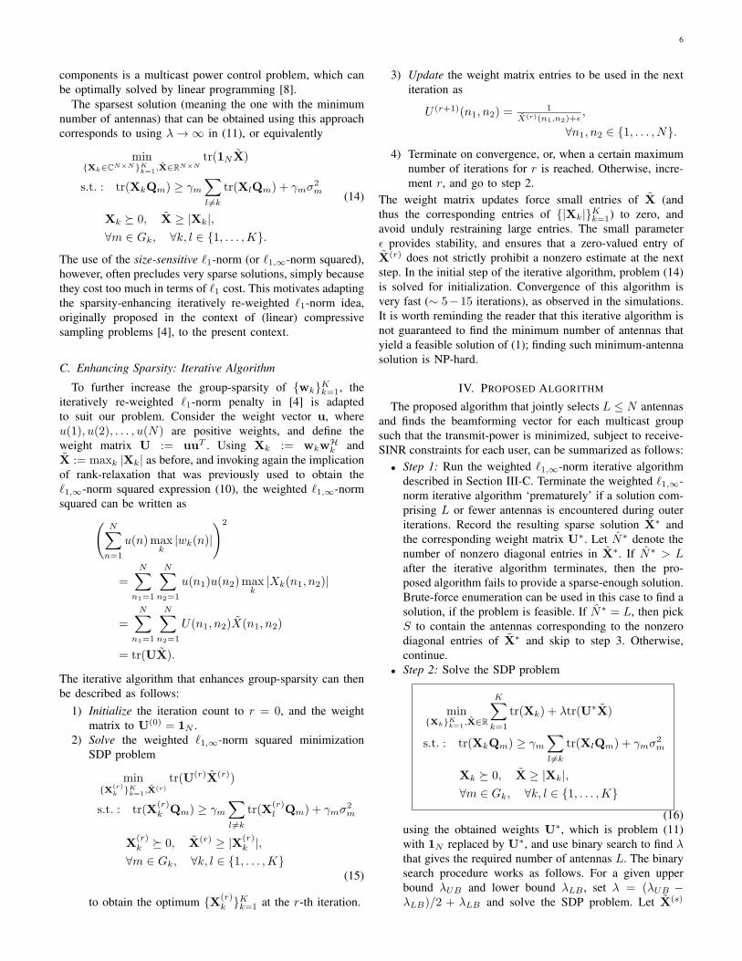
components is a multicast power control problem, which canbe optimally solved by linear programming [8].

The sparsest solution (meaning the one with the minimumnumber of antennas) that can be obtained using this approachcorresponds to using λ → ∞ in (11), or equivalently

minXk∈CN×NK

k=1,X∈RN×Ntr(1NX)

s.t. : tr(XkQm) ≥ γm∑l =k

tr(XlQm) + γmσ2m

Xk ≽ 0, X ≥ |Xk|,∀m ∈ Gk, ∀k, l ∈ 1, . . . ,K.

(14)

The use of the size-sensitive ℓ1-norm (or ℓ1,∞-norm squared),however, often precludes very sparse solutions, simply becausethey cost too much in terms of ℓ1 cost. This motivates adaptingthe sparsity-enhancing iteratively re-weighted ℓ1-norm idea,originally proposed in the context of (linear) compressivesampling problems [4], to the present context.

C. Enhancing Sparsity: Iterative Algorithm

To further increase the group-sparsity of wkKk=1, theiteratively re-weighted ℓ1-norm penalty in [4] is adaptedto suit our problem. Consider the weight vector u, whereu(1), u(2), . . . , u(N) are positive weights, and define theweight matrix U := uuT . Using Xk := wkw

Hk and

X := maxk |Xk| as before, and invoking again the implicationof rank-relaxation that was previously used to obtain theℓ1,∞-norm squared expression (10), the weighted ℓ1,∞-normsquared can be written as(

N∑n=1

u(n)maxk

|wk(n)|

)2

=

N∑n1=1

N∑n2=1

u(n1)u(n2)maxk

|Xk(n1, n2)|

=

N∑n1=1

N∑n2=1

U(n1, n2)X(n1, n2)

= tr(UX).

The iterative algorithm that enhances group-sparsity can thenbe described as follows:

1) Initialize the iteration count to r = 0, and the weightmatrix to U(0) = 1N .

2) Solve the weighted ℓ1,∞-norm squared minimizationSDP problem

minX(r)

k Kk=1,X

(r)

tr(U(r)X(r))

s.t. : tr(X(r)k Qm) ≥ γm

∑l =k

tr(X(r)l Qm) + γmσ2

m

X(r)k ≽ 0, X(r) ≥ |X(r)

k |,∀m ∈ Gk, ∀k, l ∈ 1, . . . ,K

(15)

to obtain the optimum X(r)k Kk=1 at the r-th iteration.

3) Update the weight matrix entries to be used in the nextiteration as

U (r+1)(n1, n2) =1

X(r)(n1,n2)+ϵ,

∀n1, n2 ∈ 1, . . . , N.

4) Terminate on convergence, or, when a certain maximumnumber of iterations for r is reached. Otherwise, incre-ment r, and go to step 2.

The weight matrix updates force small entries of X (andthus the corresponding entries of |Xk|Kk=1) to zero, andavoid unduly restraining large entries. The small parameterϵ provides stability, and ensures that a zero-valued entry ofX(r) does not strictly prohibit a nonzero estimate at the nextstep. In the initial step of the iterative algorithm, problem (14)is solved for initialization. Convergence of this algorithm isvery fast (∼ 5−15 iterations), as observed in the simulations.It is worth reminding the reader that this iterative algorithm isnot guaranteed to find the minimum number of antennas thatyield a feasible solution of (1); finding such minimum-antennasolution is NP-hard.

IV. PROPOSED ALGORITHM

The proposed algorithm that jointly selects L ≤ N antennasand finds the beamforming vector for each multicast groupsuch that the transmit-power is minimized, subject to receive-SINR constraints for each user, can be summarized as follows:

• Step 1: Run the weighted ℓ1,∞-norm iterative algorithmdescribed in Section III-C. Terminate the weighted ℓ1,∞-norm iterative algorithm ‘prematurely’ if a solution com-prising L or fewer antennas is encountered during outeriterations. Record the resulting sparse solution X∗ andthe corresponding weight matrix U∗. Let N∗ denote thenumber of nonzero diagonal entries in X∗. If N∗ > Lafter the iterative algorithm terminates, then the pro-posed algorithm fails to provide a sparse-enough solution.Brute-force enumeration can be used in this case to find asolution, if the problem is feasible. If N∗ = L, then pickS to contain the antennas corresponding to the nonzerodiagonal entries of X∗ and skip to step 3. Otherwise,continue.

• Step 2: Solve the SDP problem

minXkK

k=1,X∈R

K∑k=1

tr(Xk) + λtr(U∗X)

s.t. : tr(XkQm) ≥ γm∑l =k

tr(XlQm) + γmσ2m

Xk ≽ 0, X ≥ |Xk|,∀m ∈ Gk, ∀k, l ∈ 1, . . . ,K

(16)using the obtained weights U∗, which is problem (11)with 1N replaced by U∗, and use binary search to find λthat gives the required number of antennas L. The binarysearch procedure works as follows. For a given upperbound λUB and lower bound λLB , set λ = (λUB −λLB)/2 + λLB and solve the SDP problem. Let X(s)

7

denote the solution of (16) having N nonzero diagonalentries. If N = L, then find the subset of selectedantennas S corresponding to the nonzero diagonal entriesof X(s), and move to the next step. Otherwise, if N > Lthen set λLB = λ while if N < L then set λUB = λ,and repeat this step until N = L.

• Step 3: Now that L antennas have been selected, (13)is solved for the reduced-size problem, namely Xk ∈CL×LKk=1, to find the minimum power beamformingvector. If the solution, denoted as X(o)

k Kk=1, containsonly rank-one matrices, then the (suitably scaled [8])principal component of each X

(o)k is the optimal beam-

forming vector for group k. Otherwise, use the random-ization technique of [8] to generate candidate sets ofbeamforming vectors from X(o)

k Kk=1, and choose the setthat yields a minimum power solution among all feasibleones.

Note that early termination of the binary search when asolution with fewer than the desired L antennas has beenobtained will result in higher transmission power. Since λ isnon-negative, λLB can simply be set to zero. Suitable λUB canbe obtained empirically, depending primarily on ϵ (since thevalue of entries of U∗ that correspond to zero entries of X∗

is 1/ϵ as a result of the updating step of the iterative sparsity-enhancing algorithm), in addition to the network parametersN , M , K, and the channel statistics.

Although the binary search over λ may require solving (16)more than once for different values of λ until the appropriateone is found, an important advantage over the exhaustivesearch method is that the number of iterations is independentof N and L, unlike exhaustive search, which requires solving(NL

)problems of type (13). The solution obtained using the

novel algorithm occasionally coincides with that obtainedusing exhaustive search, while the transmission power increasefor the other cases is insignificant, as demonstrated in thesimulations of Section VI.

Complexity analysis. Following [8], the worst-case com-plexity of solving the SDP problem (13) using interior pointmethods is O(

√KN log(1/ε)) iterations, where ε represents

the accuracy of the solution at the algorithm’s termination, andeach iteration requires at most O(K3N6+MKN2) arithmeticoperations. The actual runtime complexity scales much slowerwith K, N , M than this worst-case bound predicts. The SDPproblem (16) includes an additional N × N auxiliary matrixand KN2 positive semidefinite constraints (as shown in theappendix), that increase the actual runtime of (16) as comparedto that of (13). However, the worst-case complexity orderremains the same. Let O(R) denote the runtime complexity ofproblem (16) (same as (11) and (15)), where R is a function ofK, N , M , and consider the complexity analysis of each of thethree steps of the proposed algorithm. In step 1, the weightedℓ1,∞-norm iterative algorithm typically terminates within lessthan 15 iterations, irrespective of the problem size. An SDP oftype (15) is solved in each iteration. Thus the total complexityof this step is O(R). In step 2, the binary search can beconsidered of constant complexity order. The number of binarysearches is typically very small with the proper choice of λUB ,

as shown in the simulations of Section VI. In each iteration,an SDP of type (16) is solved. Hence the total complexityof this step is also O(R). In step 3, one SDP of type (13)is solved (replacing N with L), with a runtime complexitythat is less than O(R). Finally, the randomization techniquethat may be used to obtain the beamforming vectors has beenanalyzed in [8], where it is shown that an ε-optimal solutioncan be obtained in O(

√K log(1/ε)) iterations, each requiring

at most O(K3+MK) arithmetic operations. Thus, the overallworst-case complexity of the proposed 3-step algorithm isO((K3.5N6.5 +MK1.5N2.5) log(1/ε)

).

V. RELEVANT EXTENSIONS

The proposed novel algorithm can easily be extended andapplied to obtain sparse solutions for a wide class of non-convex QCQP problems, where SDP relaxation is relevant.MIMO detection and sensor network localization are two suchapplications. For further details on applications where the SDPrelaxation is used, the reader is referred to [11] and referencestherein. In this section we discuss two important variationsto the multicast beamforming problem, where our proposedapproach can also be applied.

A. Limiting inter-cell or primary user interferenceSuppose there is only one multicast group (K = 1), and

consider joint antenna selection and beamformer design tominimize the transmit-power, subject to prescribed receive-SNR constraints γm for each user. In addition, consider that theinterference induced to J other users must not exceed a giventhreshold η. The channel vector from the transmit antennas tothe receive antenna of user j is denoted by gj , j ∈ 1, . . . , J,and is assumed known at the transmitter BS. The joint problemis expressed as

minw∈CN

||w||22 + λ||w||0

s.t. :|wHhm|2

σ2m

≥ γm, m = 1, . . . ,M

|wHgj |2 ≤ η, j = 1, . . . , J

(17)

which is the same as (3) with the additional interferenceconstraints for J users. Problem (17) appears in two mainscenarios: inter-cell interference mitigation in a co-channelcellular multicast setting, and secondary multicasting in acognitive underlay setting, where there is a need to limitinterference inflicted to primary users. These scenarios havebeen considered in [16], without antenna selection. Similar to[16], our formulation can be suitably modified to handle caseswhere only imperfect channel state information is available atthe BS, in the form of channel estimates with norm-boundederrors.

Returning to (17), upon replacing ||w||0 by ||w||21 and usingthe same semidefinite relaxations discussed in Section III,problem (17) can be relaxed to the SDP:

minX∈CN×N

tr(X) + λtr(1N |X|)

s.t. : tr(XQm) ≥ σ2mγm, m = 1, . . . ,M

tr(XQj) ≤ η, j = 1, . . . , J, X ≽ 0

(18)

8

where Qj := gjgHj . To select L ≤ N antennas, the proposed

algorithm in Section IV can be directly applied after addingthe constraints tr(XQj) ≤ η for j = 1, . . . , J to all the SDPproblems solved. For the final step, the randomization algo-rithm proposed in [16] can be used to find the minimum powerbeamforming vector corresponding to the selected antennas.

B. Max-Min Fair Beamforming

We now consider the related joint problem of maximizingthe minimum received SNR over all users together withantenna selection, subject to a bound P on the transmissionpower (assuming one multicast group for simplicity):

maxw∈CN

(minm

|wHhm|2

σ2m

M

m=1

)s.t. : ||w||22 ≤ P, ||w||0 ≤ L.

(19)

Problem (19) is equivalent to maximizing the beamformingdownlink achievable rate using L out of N antennas, sincein the multicast scenario, the worst-user SNR determines thecommon (multicast) rate [18]. Problem (19) was studied in[18] without the ||w||0 ≤ L constraint, and was shown to beNP-hard. Problem (19) can be equivalently re-written as

minw∈CN ,t∈R

− t+ λ||w||0

s.t. :|wHhm|2

σ2m

≥ t, m = 1, . . . ,M

||w||22 = P.

(20)

Following the same approximation steps as in Section III,problem (20) can be relaxed to the SDP:

minX∈CN×N ,t∈R

− t+ λtr(1N |X|)

s.t. : tr(XQm) ≥ σ2mt, m = 1, . . . ,M

tr(X) = P, X ≽ 0.

(21)

To select L ≤ N antennas, the proposed algorithm in SectionIV can be applied by solving the appropriate SDPs of type(21), and using the randomization algorithm proposed in [18]in the final step to extract the beamforming vector.

In closing this section, two remarks are in order on therelations between maximizing the minimum received SNR(19), the capacity of the multicast channel [7], and the antennaselection with spatial multiplexing scheme in [15]:

Remark 1. Defining X as the covariance of the transmittedsignal, the optimal solution X∗ to the rank-relaxed SDP prob-lem (21), without the sparsity inducing term (λtr(1N |X|)),is the optimal covariance that achieves the capacity of themulticast channel (maximum achievable common rate) for anN -antenna BS with full CSI at the transmitter [7]. Whereasexhaustive search is required to achieve capacity when onlyL < N antennas are utilized, the proposed algorithm inSection IV can be used to obtain an approximate, less complex,solution (by solving the appropriate SDPs of type (21)).The only difference between the multicast beamforming ratemaximization and the multicast channel capacity is that Xis restricted to be rank one with beamforming (and the

randomization algorithm proposed in [18] is needed to extractthe beamforming vector from the optimal X), whereas thereis no such restriction (and no approximation) for the capacity-achieving transmit covariance. The role of the rank restrictionand the use of the sparsity inducing ℓ1-norm squared approx-imation are illustrated in Section VI-C.

Remark 2. In the absence of CSI at the transmitter, thealternative is to transmit using a spatially white covariance,i.e., X = P

N IN , where P is the total transmission powerand X denotes the covariance of the transmitted signal [7].An antenna selection scheme has been proposed in [15]for maximizing the minimum received SNR based on thissetup. When utilizing a subset of antennas S of size L, thetransmission power is equally divided among all L antennasyielding an SNR for the m-th user SNRm = P

L

∑n∈S |hm(n)|2

σ2m

.From all possible antenna subsets S of size L, the selectedsubset S∗ is the one maximizing the minimum SNR acrossall users, namely

S∗ = arg maxS∈S

minm∈1,...,M

P

L

∑n∈S |hm(n)|2

σ2m

where S is the set of all(NL

)possible antenna subsets of

size L. This antenna selection scheme requires knowledge ofthe channel gain corresponding to each transmit antenna atthe transmitter (|hm(n)|2) for each user, in addition to ex-haustively searching through all

(NL

)different antenna subset

S selections. The results of [7] imply that transmitting withspatially white covariance will outperform beamforming (interms of spectral efficiency) when M ≫ L, because everybeamforming direction will likely be nearly orthogonal toat least one user’s channel, whereas beamforming performssignificantly better (very close to the multicast capacity) forrelatively large L. Attaining this rate with spatially whitecovariance is a challenge since it requires complex multi-stream Shannon encoding and decoding at long block lengths,also implying long decoding delay that is not suitable forstreaming media multicast. Beamforming, on the other hand,requires far simpler encoding and decoding. The performanceof our proposed beamforming based algorithm is comparedwith that of [15] in Section VI-C.

VI. SIMULATED TESTS

To test the proposed SDP-based algorithms, YALMIP wasused. YALMIP is a modeling language for optimization prob-lems that is implemented as a free toolbox for MATLAB [10],and uses SeDuMi, a MATLAB implementation of second-order interior-point methods, for the actual computations [19].The novel algorithm was tested with two channel types;Rayleigh fading channels and Vandermonde channels corre-sponding to a far-field ULA setup. Throughout this section,the noise variance for all users was set to σ2 = 1.

A. Single Multicast Group

We first consider a single multicast group, and set theminimum required SNR to γ = 1 at all users.

9

Rayleigh fading with N = 8 antennas. The first simulationsetup included a BS with N = 8 transmit-antennas broadcast-ing a common message to M = 16 receivers. Independentidentically distributed (i.i.d.) Rayleigh fading channel vectorshmMm=1 were generated, each with i.i.d. entries circularlysymmetric zero-mean complex Gaussian random variablesof variance 1. To gain insight, detailed results are providedfirst for a single “typical” channel realization, which allowscomparing the selected antenna subsets with the baselineexhaustive search solution. Running the weighted ℓ1-normiterative algorithm described in Section III-C results in thesparsest solution of N∗ = 1 antenna, which corresponds toselecting antenna number 5. This result is obtained when theiterative algorithm converges after 8 iterations. It is worthnoting that after the initial step of the iterative weighted ℓ1-norm algorithm (which is equivalent to solving problem (14)),the resulting sparse solution has N = 6 antennas, many morethan the single antenna solution obtained after the iterativeweighted ℓ1-norm algorithm terminates.

Table I summarizes the results obtained using the novelalgorithm and by exhaustively searching over possible antennasubset selections for this representative channel realization.The required number of antennas to be selected (or, theavailable number of RF chains) L is listed in column 1. Thesubset of selected antennas is given in columns 2 and 6 for theproposed algorithm and exhaustive search, respectively. Theminimum transmit-power corresponding to each L is listed incolumns 3 and 7 (in dBm units). The increase of transmissionpower (compared to the case of using all N = 8 antennas)due to antenna selection is given in columns 4 and 8 (in dBunits). Finally, the total number of SDP problems solved inorder to obtain the required solution is shown in columns 5and 9.

The results in Table I demonstrate that as the number ofantennas selected for transmission decreases (as the solutionbecomes more sparse) the corresponding minimum trans-mission power increases, due to the decrease in degrees offreedom, as expected. Interestingly, the simulations suggestthat the number of transmit antennas can be significantlyreduced at only a small price in terms of excess transmissionpower. Halving the number of antennas from 8 to 4, forexample, entails only 1.11 dB extra power. Comparing withthe exhaustive search results, one can verify that exhaustivesearch slightly outperforms the proposed algorithm only forthe cases of L = 5 and L = 6 antennas (by less than 0.1 dB),by selecting different antenna subsets. However, the numberof SDP problems that must be solved for the exhaustive searchis significantly larger. The maximum number of iterationsrequired for the binary search process, namely step 2 in theproposed algorithm, is 7 - these are needed to select L = 7antennas, where 1 SDP problem is solved for step 1, 7 forstep 2, and 1 for the final step, yielding a worst-case totalof 9 SDP problems. On the other hand, the exhaustive searchalgorithm requires solving

(84

)= 70 SDP problems to select

L = 4 antennas.Table II reports the average and maximum increase in

transmission power (compared to the case of using all N = 8antennas) that correspond to selecting L antennas for the

2 3 4 5 6 7 80

1

2

3

4

5

6

Selected Antennas

Ext

ra P

ower

(dB

)

Average Results (N=8, M=16)

Exh. Search

Prop. Alg.

Fixed

Robust δ = 0.005

Robust δ = 0.1

Fig. 1. The necessary extra power versus L for N = 8 antennas and a singlemulticast group with M = 16 users in a Rayleigh fading environment.

proposed algorithm, the exhaustive search, and the case wherethe number of available antennas is only L (not N ) suchthat no antenna selection is performed (this is equivalent torandomly selecting the L antennas). In addition, the aver-age and maximum number of SDP problems solved for theproposed algorithm and exhaustive search are reported. Fora better visual comparison, Fig. 1 plots the average increasein transmission power versus L for the compared schemes(corresponding to columns 2, 6 and 9 of Table II). The resultsare obtained for 100 different Rayleigh channel realizations.The main conclusions from Table II and Fig. 1 are summarizedas follows:

1) The number of transmit antennas can be considerablyreduced at a relatively small cost in terms of excesstransmission power. If we halve the number of antennas,the transmission power increases by only 1 dB, on av-erage, to satisfy the SNR constraints using the proposedalgorithm.

2) Compared to the exhaustive search, the proposed algo-rithm incurs much lower complexity (measured in termsof the number of SDP problems solved) at a very smalladditional power cost. The difference in power is lessthan 1 dB, on average.

3) If only L RF transmission chains are available at theBS, increasing the number of transmit antennas N(from which only L are activated) results in a reductionin transmission power due to the additional diversity.For example, if only 4 RF chains and 4 antennas areavailable (N = L = 4), 1.2 dB more transmission poweris required compared to having the option of selecting4 out of 8 antennas using the proposed algorithm, onaverage.

Rayleigh fading with N = 16 antennas. In Fig. 2, weconsider N = 16 antennas and M = 32 users, again assumingi.i.d. Rayleigh fading across antennas and users. The figuredepicts the average increase in transmission power (comparedto the case of using all N = 16 antennas) versus L. If we halvethe number of selected antennas (L = 8), the transmissionpower increases by only 1.5 dB to satisfy the SNR constraintsusing the proposed algorithm, whereas if only 8 antennaswere installed instead of 16 (i.e. no antenna selection), anadditional 0.7 dB transmission power would be necessary

10

Proposed Algorithm Exhaustive SearchL Selected Power Power inc. Total Selected Power Power inc. Total

antennas S (dBm) (dB) SDP’s antennas S (dBm) (dB) SDP’s8 1,. . . ,8 30.82 0 1 1,. . . ,8 30.82 0 17 1,2,3,4,5,7,8 31.16 0.34 9 1,2,3,4,5,7,8 31.16 0.34 86 2,3,4,5,7,8 31.81 0.99 2 1,2,4,5,7,8 31.75 0.93 285 2,3,4,5,7 31.84 1.02 5 2,4,5,7,8 31.80 0.98 564 2,4,5,7 31.92 1.11 3 2,4,5,7 31.92 1.11 703 2,5,7 32.42 1.6 6 2,5,7 32.42 1.6 562 5,7 33.86 3.04 7 5,7 33.86 3.04 281 5 35.78 4.96 8 5 35.78 4.96 8

TABLE IPERFORMANCE OF THE PROPOSED ALGORITHM AND THE EXHAUSTIVE SEARCH ALGORITHM FOR A PARTICULAR CHANNEL REALIZATION FOR

DIFFERENT ANTENNA SELECTIONS L, FOR N = 8 ANTENNA BS AND A SINGLE MULTICAST GROUP WITH M = 16 USERS.

Proposed Algorithm Exhaustive Search Fixed AntennasL Power Inc. (dB) Total SDP’s Power Inc. (dB) Total SDP’s Power Inc. (dB)

Avg. Max. Avg. Max. Avg. Max. Avg. Max.6 0.22 2.7 7.5 17 0.1 1.12 28 0.9 3.14 1 3.2 4.3 11 0.5 2.3 70 2.2 4.82 2.9 6.7 4.4 9 2.1 6.7 28 5.5 11.8

TABLE IIPERFORMANCE COMPARISON BETWEEN THE PROPOSED ALGORITHM, EXHAUSTIVE SEARCH AND NO ANTENNA SELECTION, FOR N = 8 ANTENNA BS

AND A SINGLE MULTICAST GROUP WITH M = 16 USERS IN A RAYLEIGH FADING ENVIRONMENT.

4 6 8 10 12 14 160

1

2

3

4

5

6

Number of Selected Antennas

Ext

ra P

ower

(dB

)

Average Results (N=16 and M=32)

Fixed

Prop. Alg.

Fig. 2. The necessary extra power versus L for N = 16 antennas and asingle multicast group with M = 32 users in a Rayleigh fading environment.

(compared to the proposed algorithm), on average. The resultsfor the exhaustive search algorithm are not included becauseof its prohibitive complexity. If, for example, it is requiredto select L = 8 antennas, exhaustive search requires solving(168

)= 12, 870 SDP problems per channel realization, which is

clearly prohibitive. On the other hand, the proposed algorithmrequired solving less than 7 SDP problems for L = 8, onaverage.

Rayleigh fading with N = 100 antennas. In Fig. 3, weconsider a scenario with a large number of antennas and users(N = 100, M = 100), again assuming i.i.d. Rayleigh fading.The figure shows the average additional transmit-power neededusing the proposed algorithm, which is 1-2 dB less than thetransmit-power needed when the first L antennas are blindlyselected, for all values of L considered. Read in a differentway, the proposed algorithm uses far fewer transmit antennasfor the same transmit-power. Of course, it is computationallyprohibitive to apply exhaustive search in this scenario. Note

15 20 25 30 35 40 45 500

1

2

3

4

5

6

Number of Selected Antennas (L)

Ext

ra P

ower

(dB

) N=100, M=100

Prop. alg.

Fixed sel.

Fig. 3. The necessary extra power versus L with N = 100 and M = 100in a Rayleigh fading environment.

that the gains offered by the proposed algorithm are relativelysmall when the number of users is relatively large and thechannel is i.i.d. across antennas and users - because the lawof large numbers kicks in. The situation is different when Mis small. For example, with N = 100 antennas to choosefrom, M = 2 users, and L = 2 antennas to be selected, themaximum transmit-power using our proposed algorithm, over1000 Rayleigh channel realizations, was 34.7dBm (23.9dBmon average), whereas the maximum transmit-power whenblindly selecting the first 2 antennas was 58.9dBm (30.3dBmon average). This means that the proposed algorithm can saveup to approximately 24dB in transmit-power compared to fixedantenna selection in this setting.

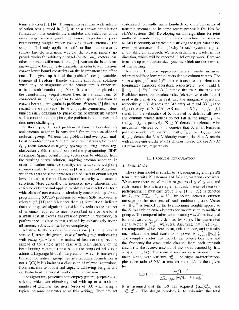
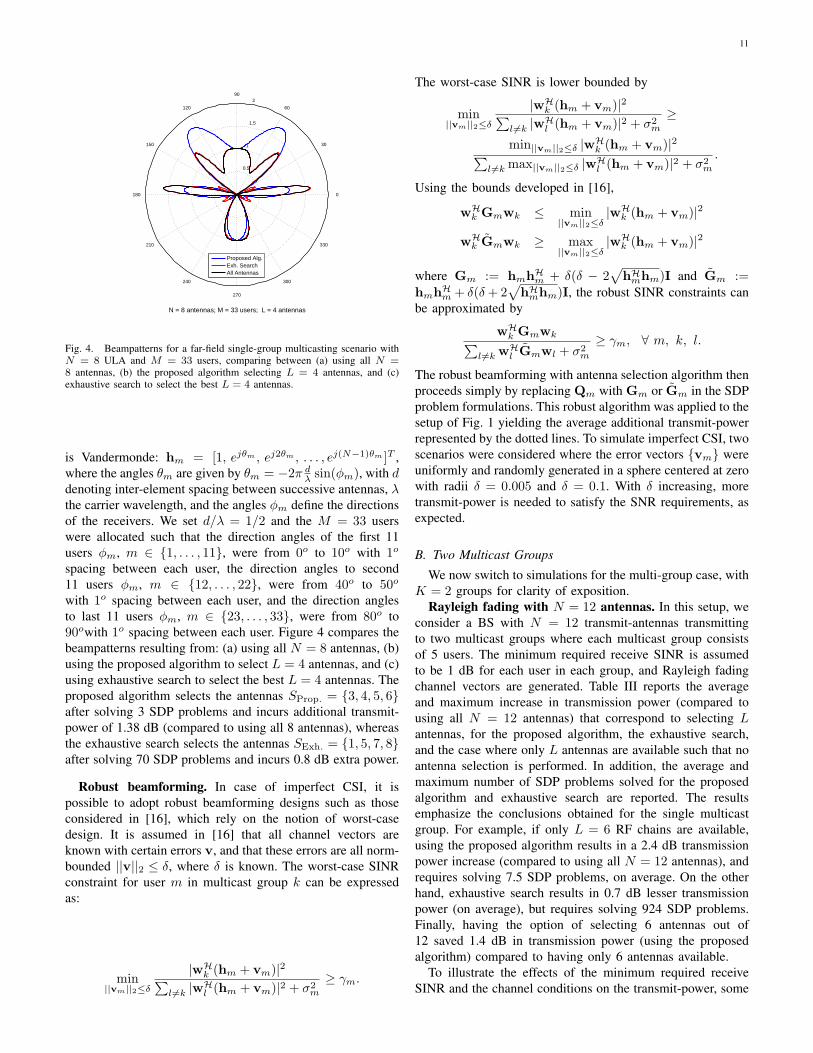
Far-field beamforming with N = 8 ULA. Figure 4illustrates the beampatterns for a particular far-field multi-casting scenario with N = 8 ULA antennas and M = 33users. The N × 1 complex channel vector for each user m

11

0.5

1

1.5

2

30

210

60

240

90

270

120

300

150

330

180 0

N = 8 antennas; M = 33 users; L = 4 antennas

Proposed Alg.Exh. SearchAll Antennas

Fig. 4. Beampatterns for a far-field single-group multicasting scenario withN = 8 ULA and M = 33 users, comparing between (a) using all N =8 antennas, (b) the proposed algorithm selecting L = 4 antennas, and (c)exhaustive search to select the best L = 4 antennas.

is Vandermonde: hm = [1, ejθm , ej2θm , . . . , ej(N−1)θm ]T ,where the angles θm are given by θm = −2π d

λ sin(ϕm), with ddenoting inter-element spacing between successive antennas, λthe carrier wavelength, and the angles ϕm define the directionsof the receivers. We set d/λ = 1/2 and the M = 33 userswere allocated such that the direction angles of the first 11users ϕm, m ∈ 1, . . . , 11, were from 0o to 10o with 1o

spacing between each user, the direction angles to second11 users ϕm, m ∈ 12, . . . , 22, were from 40o to 50o

with 1o spacing between each user, and the direction anglesto last 11 users ϕm, m ∈ 23, . . . , 33, were from 80o to90owith 1o spacing between each user. Figure 4 compares thebeampatterns resulting from: (a) using all N = 8 antennas, (b)using the proposed algorithm to select L = 4 antennas, and (c)using exhaustive search to select the best L = 4 antennas. Theproposed algorithm selects the antennas SProp. = 3, 4, 5, 6after solving 3 SDP problems and incurs additional transmit-power of 1.38 dB (compared to using all 8 antennas), whereasthe exhaustive search selects the antennas SExh. = 1, 5, 7, 8after solving 70 SDP problems and incurs 0.8 dB extra power.

Robust beamforming. In case of imperfect CSI, it ispossible to adopt robust beamforming designs such as thoseconsidered in [16], which rely on the notion of worst-casedesign. It is assumed in [16] that all channel vectors areknown with certain errors v, and that these errors are all norm-bounded ||v||2 ≤ δ, where δ is known. The worst-case SINRconstraint for user m in multicast group k can be expressedas:

min||vm||2≤δ

|wHk (hm + vm)|2∑

l =k |wHl (hm + vm)|2 + σ2

m

≥ γm.

The worst-case SINR is lower bounded by

min||vm||2≤δ

|wHk (hm + vm)|2∑

l =k |wHl (hm + vm)|2 + σ2

m

≥

min||vm||2≤δ |wHk (hm + vm)|2∑

l =k max||vm||2≤δ |wHl (hm + vm)|2 + σ2

m

.

Using the bounds developed in [16],

wHk Gmwk ≤ min

||vm||2≤δ|wH

k (hm + vm)|2

wHk Gmwk ≥ max

||vm||2≤δ|wH

k (hm + vm)|2

where Gm := hmhHm + δ(δ − 2

√hHmhm)I and Gm :=

hmhHm + δ(δ+2

√hHmhm)I, the robust SINR constraints can

be approximated by

wHk Gmwk∑

l =k wHl Gmwl + σ2

m

≥ γm, ∀ m, k, l.

The robust beamforming with antenna selection algorithm thenproceeds simply by replacing Qm with Gm or Gm in the SDPproblem formulations. This robust algorithm was applied to thesetup of Fig. 1 yielding the average additional transmit-powerrepresented by the dotted lines. To simulate imperfect CSI, twoscenarios were considered where the error vectors vm wereuniformly and randomly generated in a sphere centered at zerowith radii δ = 0.005 and δ = 0.1. With δ increasing, moretransmit-power is needed to satisfy the SNR requirements, asexpected.

B. Two Multicast Groups

We now switch to simulations for the multi-group case, withK = 2 groups for clarity of exposition.

Rayleigh fading with N = 12 antennas. In this setup, weconsider a BS with N = 12 transmit-antennas transmittingto two multicast groups where each multicast group consistsof 5 users. The minimum required receive SINR is assumedto be 1 dB for each user in each group, and Rayleigh fadingchannel vectors are generated. Table III reports the averageand maximum increase in transmission power (compared tousing all N = 12 antennas) that correspond to selecting Lantennas, for the proposed algorithm, the exhaustive search,and the case where only L antennas are available such that noantenna selection is performed. In addition, the average andmaximum number of SDP problems solved for the proposedalgorithm and exhaustive search are reported. The resultsemphasize the conclusions obtained for the single multicastgroup. For example, if only L = 6 RF chains are available,using the proposed algorithm results in a 2.4 dB transmissionpower increase (compared to using all N = 12 antennas), andrequires solving 7.5 SDP problems, on average. On the otherhand, exhaustive search results in 0.7 dB lesser transmissionpower (on average), but requires solving 924 SDP problems.Finally, having the option of selecting 6 antennas out of12 saved 1.4 dB in transmission power (using the proposedalgorithm) compared to having only 6 antennas available.

To illustrate the effects of the minimum required receiveSINR and the channel conditions on the transmit-power, some

12

1

2 30

210

60

240

90

270

120

300

150

330

180 0

Two Multicast GroupsN = 8 antennas; M = 32 users; L = 4 antennas

All AntennasGroup 2

Prop. Alg.Group 2

All Antennas Group 1

Prop. Alg.Group 1

Fig. 5. Beampatterns for a far-field two-group multicasting scenario withN = 8 ULA and M = 32 users, comparing between using all N = 8antennas and the proposed algorithm selecting L = 4 antennas.

variations of the last setup were considered. For a minimumrequired receive-SINR = 3 dB per user in each group,the average transmit-power using all 12 antennas was 31.2dBm, whereas the average transmit-power after selecting 6antennas increased to 33.6 dBm. To simulate for better channelconditions, each user’s channel was multiplied by a constantc = 5. As a result, the average transmit-power decreased to17.2 dBm when all 12 antennas were utilized, and to 19.6 dBmwhen 6 antennas were selected. For a 12 dB minimum SINR,the average transmit-power was 41 dB when all antennas wereused, and 44.4 dBm when 6 antennas were selected. Wheneach user’s channel was multiplied by c = 5, the averagetransmit-power decreased to 27.2 dBm when all 12 antennaswere utilized, and to 30 dBm when 6 antennas were selected.

Far-field beamforming with N = 8 ULA. Figure 5 illus-trates the beampatterns for a particular far-field multicastingscenario with N = 8 ULA and M = 32 users. The users areequally divided into two multicast groups. The 16 users of thefirst multicast group G1 have direction angles ϕm (m ∈ G1)from 0o to 30o with 2o spacing between each user, whilethe 16 users of the second multicast group G2 have directionangles ϕm (m ∈ G2) from 60o to 90o with 2o spacing betweeneach user. The minimum required receive-SINR was assumedto be 3 dB for each user, and we set d/λ = 1/2. Figure5 compares the beampattern resulting from using all N = 8antennas with that resulting from using the proposed algorithmto select L = 4 antennas. For this setting, the proposedalgorithm selects the same 4 antennas as the exhaustive searchyielding the same beampattern. The proposed algorithm (andexhaustive search) incurs additional transmit-power of only1.66 dB (compared to using all 8 antennas).

C. Max-min-fair Beamforming and Spectral Efficiency Con-siderations

Here, we consider the problem of maximizing the minimumreceived SNR over all users with antenna selection, whichis described in Section V-B. In this setup, we considered a

2 3 4 5 6 7 8 9 102.2

2.4

2.6

2.8

3

3.2

3.4

3.6

3.8

4

4.2

Selected Antennas (L)

Ave

rage

Spe

ctra

l Effi

cien

cy (

bps/

Hz)

(e) White Cov. + Exh. Srch.

(d) BF + Sparse Approx.

(c) BF + Exh. Srch.

(b) Capacity + Sparse Approx.

(a) Capacity + Exh. Srch.

Fig. 6. Average spectral efficiency versus L for N = 10 antennas andM = 16 users.

BS with N = 10 antennas, M = 16 users, Rayleigh fadingchannels and the transmission power was bounded belowP = 10 dB. Figure 6 compares the following schemes: (a)Capacity achieving transmit-covariance with exhaustive searchantenna selection (which corresponds to the multicast chan-nel capacity with antenna selection); (b) Capacity achievingtransmit-covariance with sparsity-inducing ℓ1-norm squaredapproximation; (c) Beamforming with exhaustive search an-tenna selection; (d) Beamforming with sparsity-inducing ℓ1-norm squared approximation; and, (e) Spatially white transmit-covariance with exhaustive search antenna selection, as con-sidered in [15]. Note that for (c) and (d), beamforming impliesrank-one transmit-covariance. For each scheme, the (average)maximum achievable rate per unit bandwidth (which is theaverage spectral efficiency given by Eh[log2(1 + γ(h))] inbps/Hz units, where γ(h) is the minimum received SNRamong all M users for each channel realization, and Eh

denotes Monte-Carlo expectation over all Rayleigh fadingchannel realizations) is plotted versus the number of selectedantennas L.

Figure 6 confirms that the previous conclusions for minimiz-ing the transmission power with SNR constraints are also validwhen antenna selection is jointly considered. For example, theaverage spectral efficiency with beamforming decreases by lessthan 0.5 bps/Hz when L = 4 antennas are selected comparedto using all N = 10 antennas, which is an insignificantdecrease compared to the reduction in RF chains. Moreover,the figure shows that (b) and (d) are within 0.25 bps/Hz lessspectral efficiency than (a) and (c), respectively. On the otherhand, (b) and (d) required solving less than 5 SDP problems,on average, while (a) and (c) required solving 210 SDP prob-lems to select L = 4 or L = 6 antennas. This emphasizes theeffectiveness of using the sparsity-inducing ℓ1-norm squaredapproximation. Finally, we see that (c) outperforms (e), or inother words beamforming outperforms using spatially whitetransmit-covariance, since L is not very small compared toM . The performance of beamforming becomes significantlybetter as L increases, whereas this advantage vanishes forsmaller L. The reason, as explained in [7], is that everybeamforming direction will be nearly orthogonal to at least

13

Proposed Algorithm Exhaustive Search Fixed AntennasL Power Inc. (dB) Total SDP’s Power Inc. (dB) Total SDP’s Power Inc. (dB)

Avg. Max. Avg. Max. Avg. Max. Avg. Max.10 0.43 0.7 9 20 0.27 0.4 66 0.85 28 1 1.55 11.5 25 0.81 0.97 495 2.1 3.356 2.4 2.8 7.5 22 1.7 2.3 924 3.8 6.74 4.4 5.92 5.5 25 3.7 4.3 495 7.6 9.8

TABLE IIIPERFORMANCE COMPARISON BETWEEN THE PROPOSED ALGORITHM, EXHAUSTIVE SEARCH AND NO ANTENNA SELECTION, FOR N = 12 ANTENNA BS

AND TWO MULTICAST GROUPS WITH |G1| = 5 AND |G2| = 5 IN A RAYLEIGH FADING ENVIRONMENT.

one user’s channel with high probability when M ≫ L.

VII. CONCLUSIONS

We studied the joint problem of multicast beamformingto multiple multicast groups with antenna selection. Theobjective is to select sparse beamforming vectors such thatthe transmission power is minimized, subject to the SINRconstraints at all subscribers. Instead of using the ℓ1-norm topromote sparsity, we argued that the mixed ℓ1,∞-norm squaredoffers a more prudent group-sparsity inducing regularizationfor our purposes. The reason is that it naturally (and elegantly)yields a semidefinite relaxation that is similar in spirit tothe corresponding one for the baseline multicasting problemwithout antenna selection, considered in [18]. One interestingresult is that the number of transmit antennas can be consid-erably reduced with only minimal increase in the transmissionpower. We also showed that our proposed algorithm performsjoint antenna selection and weight optimization at significantlylower complexity compared to using exhaustive search forantenna selection, and at negligible excess power. The novelalgorithm can be combined with admission control [12], andcan be easily modified to obtain sparse solutions for a wideclass of non-convex QCQP problems, and applications whereSDP relaxation is relevant.

Finally, developing custom algorithms for joint multicastbeamforming and antenna selection for Massive MIMO sys-tems [26] is of interest. We have preliminary work in thisdirection; but striking the right balance between performanceand complexity in the large system regime requires a verydifferent approach from the one presented herein. We willtherefore report these findings in follow-up work.

APPENDIX

Proof of Proposition 1: Consider the single multicast groupscenario. In this case, the ℓ1,∞-norm reduces to the ℓ1-normand problem (8) is expressed as

minw∈CN

||w||22 + λ||w||21

s.t. : |wHhm|2 ≥ 1, m = 1, . . . ,M(22)

where hm is normalized by√σ2mγm. Using Qm := hmhH

m

and X := wwH, problem (22) is equivalent to

minX∈CN×N ,Y∈RN×N

tr(X) + λtr(1NY)

s.t. : tr(XQm) ≥ 1, m = 1, . . . ,M

|X(i, j)| ≤ Y (i, j), ∀i, j ∈ 1, . . . , NX ≽ 0, rank(X) = 1.

(23)

In order to transform (23) from the complex domain to thereal domain, we define wR := ℜw, wI := ℑw, z :=[wT

R wTI ]

T , and Z := zzT such that Z ∈ R2N×2N . Now, itis easy to see that ℜX(i, j) = Z(i, j) + Z(N + i,N + j)and ℑX(i, j) = −Z(i,N + j) + Z(N + i,N). Thus, theconstraints |X(i, j)| ≤ Y (i, j), ∀i, j are equivalent to

|| (Z(i, j) + Z(N + i,N + j))+√−1 (−Z(i,N + j) + Z(N + i,N)) ||2 ≤ Y (i, j).

These constraints can be expressed as the positive semidefiniteconstraints (24), ∀i, j, in the real domain. The channel matrixQm can be transformed to the real domain by defining gm :=[ℜhmT ℑhmT ]T , gm := [ℑhmT − ℜhmT ]T , andthe 2N × 2N rank-2 matrix Qm := gmgT

m + gmgTm. Hence,

problem (23) can be expressed in the real domain as

minZ∈R2N×2N ,Y∈RN×N

tr(Z) + λtr(1NY)

s.t. : tr(ZQm) ≥ 1, m = 1, . . . ,M

Cij ≽ 0, ∀i, j ∈ 1, . . . , NZ ≽ 0, rank(Z) = 1.

(25)

Finally, defining Z := diag(Z Y C11 C12 . . . C1N C21 . . . CNN )

such that Z ∈ RN×N , where N := 3N + 2N2,

A :=

I2N 02N×N 02N×2N2

0N×2N λ.1N 0N×2N2

02N2×2N 02N2×N 02N2×2N2

,

and

Qm :=

[−Qm 02N×(N+2N2)

0(N+2N2)×2N 0(N+2N2)×(N+2N2)

]

14

Cij :=

[Y (i, j)− Z(i, j)− Z(N + i,N + j) −Z(i,N + j) + Z(N + i, j)

−Z(i,N + j) + Z(N + i, j) Y (i, j) + Z(i, j) + Z(N + i,N + j)

]≽ 0. (24)

problem (25) can be expressed as

minZ∈RN×N

tr(ZA)

s.t. : tr(ZQm) + 1 ≤ 0, m = 1, . . . ,M

tr(ZE

(11)ij

)= 0, tr

(ZE

(12)ij

)= 0

tr(ZE

(21)ij

)= 0, tr

(ZE

(22)ij

)= 0,

∀i, j ∈ 1, . . . , N, Z ≽ 0, rank(Z) = 1(26)

where E(11)ij , E(22)

ij , E(12)ij and E

(21)ij provide the four entries

of Cij , for each i and j, by ensuring that:

Z (3N + 2(i− 1)N + 2j − 1, 3N + 2(i− 1)N + 2j − 1)

= Z(2N + i, 2N + j)− Z(i, j)− Z(N + i,N + j)

Z (3N + 2(i− 1)N + 2j, 3N + 2(i− 1)N + 2j)

= Z(2N + i, 2N + j) + Z(i, j) + Z(N + i,N + j)

Z (3N + 2(i− 1)N + 2j − 1, 3N + 2(i− 1)N + 2j)

= −Z(i,N + j) + Z(N + i, j)

Z (3N + 2(i− 1)N + 2j, 3N + 2(i− 1)N + 2j − 1)

= −Z(i,N + j) + Z(N + i, j).

By dropping the rank(Z) = 1 constraint, problem (26) isin the standard SDP form. Defining the N × 1 vector z :=[wT

R wTI yT cT11 cT12 . . . cT1N cT21 . . . cTNN ]T where y is

an N × 1 auxiliary vector and cij is a 2× 1 vector, problem(26), which is equivalent to the original problem (22), can beexpressed in the following standard QCQP form:

minz

zTAz

s.t. : zT Qmz+ 1 ≤ 0, m = 1, . . . ,M

zTE(11)ij z = 0, zTE

(12)ij z = 0

zTE(21)ij z = 0, zTE

(22)ij z = 0, ∀i, j ∈ 1, . . . , N.

(27)

Introducing the Lagrange multipliers µ (M ×1), ν (4N2×1), and defining l := 4(i− 1)N + j and

P := A+M∑

m=1

µmQm+

∑Ni=1

∑Nj=1

(νlE

(11)ij + νl+NE

(12)ij + νl+2NE

(21)ij + νl+3NE

(22)ij

),

the Lagrangian of problem (27) is L(z,µ,ν) = zTPz +∑Mm=1 µm, and the dual problem is

maxµ≽0,ν

infzL(z,µ,ν).

It is easy to see that

infzzTPz+

M∑m=1

µm =

∑Mm=1 µm if P ≽ 0

−∞ otherwise .

The dual problem can thus be expressed as

maxµ,ν

M∑m=1

µm

s.t. : P ≽ 0, µm ≥ 0, m = 1, . . . ,M

(28)

which is an easily solvable convex SDP. Finally, it is easyto see that the dual of the SDP (28), which is the bi-dualof (22), is problem (23) after dropping the rank(X) = 1constraint [22]. Also, the dual of the rank-relaxed problem(23) is problem (28).

The duality results are easily extended to the multiplemulticast groups scenario by extending the matrix Z toZkKk=1 and adding K replicates for the positive semidefiniteconstraints Cij ≽ 0, ∀i, j ∈ 1, . . . , N, in (25) correspondingto each Zk, ∀k ∈ 1, . . . ,K. The rest of the steps are astraightforward extension from the single multicast group case.

REFERENCES

[1] F. Bach, R. Jenatton, J. Mairal and G. Obozinski, “Optimizationwith sparsity-inducing penalties,” Technical Report [Available at:arxiv.org/pdf/1108.0775v2.pdf], August 2011.

[2] M. Bengtsson and B. Ottersten, “Optimal and suboptimal transmitbeamforming,” in Handbook of Antennas in Wireless Communications,L. C. Godara, Ed., Boca Raton, FL: CRC, 2001, ch. 18.

[3] S. Boyd and L. Vandenberghe, Convex Optimization. Cambridge, U.K.:Cambridge Univ. Press, 2004.

[4] E. Candes, M. Wakin, and S. Boyd, “Enhancing sparsity by reweightedℓ1 minimization,” J. Fourier Analysis and Applications, vol. 14, no. 5,pp. 877–905, Dec. 2008.

[5] J. de Andrade Jr., M. Campos, and J. Apolinario, “Sparse solutions forantenna arrays,” in Proc. XXIX Simposio Brasileiro de Telecomunica-coes, Curitiba, Brazil, Oct. 2-5, 2011.

[6] A. Dua, K. Medepalli, and A. Paulraj, “Receive antenna selectionin MIMO systems using convex optimization,” IEEE Trans. WirelessCommunications, vol. 5, no. 9, pp. 2353–2357, Sept. 2006.

[7] N. Jindal and Z. Q. Luo, “Capacity limits of multiple antenna multi-cast,” in Proc. IEEE Int. Symp. Inf. Theory, pp. 1841–1845, Seattle,Washington, July 9-14, 2006.

[8] E. Karipidis, N.D. Sidiropoulos, and Z.-Q. Luo, “Quality of serviceand max-min-fair transmit beamforming to multiple co-channel multicastgroups,” IEEE Trans. Signal Processing, vol. 56, no. 3, pp. 1268–1279,March 2008.

[9] E. Karipidis, N.D. Sidiropoulos, and Z.-Q. Luo, “Far-field multicastbeamforming for uniform linear antenna arrays,” IEEE Trans. SignalProcessing, vol. 55, no. 10, pp. 4916–4927, Oct. 2007.

[10] J. Lofberg, “Yalmip: A toolbox for modeling and optimization inMATLAB,” in Proc. CACSD, Taipei, Sep. 4, 2004.

[11] Z.-Q. Luo, W. Ma, A. So, Y. Ye, and S. Zhang, “Semidefinite relaxationof quadratic optimization problems,” IEEE Signal Processing Magazine,vol. 27, no. 3, pp. 20–34, May 2010.

[12] E. Matskani, N.D. Sidiropoulos, Z.-Q. Luo, L. Tassiulas, “Efficient batchand adaptive approximation algorithms for joint multicast beamformingand admission control,” IEEE Trans. on Signal Processing, vol. 57, no.12, pp. 4882–4894, Dec. 2009.

[13] O. Mehanna, N. D. Sidiropoulos, and G. B. Giannakis, “Multicastbeamforming with antenna selection,” Proc. of 13th Workshop on SignalProcessing Advances in Wireless Communications, Cesme, Turkey, June17-20, 2012.

[14] S. Nai, W. Ser, Z. Yu, and H. Chen, “Beampattern synthesis for linearand planar arrays with antenna selection by convex optimization,” IEEETrans. Antennas and Propagation, vol. 58, no. 12, pp. 3923–3930, Dec.2010.

15

[15] S. Park and D. Love, “Capacity limits of multiple antenna multicastingusing antenna subset selection,” IEEE Transactions on Signal Process-ing, vol. 56, no. 6, pp. 2524–2534, June 2008.

[16] K. Phan, S. Vorobyov, N.D. Sidiropoulos, and C. Tellambura, “Spectrumsharing in wireless networks via QoS-aware secondary multicast beam-forming,” IEEE Trans. Signal Processing, vol. 57, no. 6, pp. 2323–2335,June 2009.

[17] S. Sanayei and A. Nostratinia, “Antenna selection in MIMO systems,”IEEE Communications Magazine, pp. 68–73, Oct. 2004.

[18] N.D. Sidiropoulos, T. Davidson, and Z.-Q. Luo, “Transmit beamformingfor physical layer multicasting,” IEEE Trans. Signal Processing, vol. 54,no. 6, part 1, pp. 2239–2251, June 2006.

[19] J. Sturm, “Using SeDuMi 1.02, a MATLAB toolbox for optimizationover symmetric cones,” Optimization Methods and Software, vol. 11,no. 1, pp. 625–653, 1999.

[20] R. Tibshirani, “Regression shrinkage and selection via the Lasso,” J.Royal. Statist. Soc B., vol. 58, no. 1, pp. 267-288, 1996.

[21] B. Turlach, W. N. Venables, and S. J. Wright, “Simultaneous variableselection,” Technometrics, vol. 47, no. 3, pp. 349–363, 2005.

[22] L. Vandenberghe and S. Boyd, “Semidefinite programming,” SIAM Rev.,vol. 38, pp. 49–95, 1996.

[23] H. Wolkowicz, “Relaxations of Q2P”, Chapter 13.4 in Handbook ofSemidefinite Programming: Theory, Algorithms, and Applications, H.Wolkowicz, R. Saigal, L. Vandenberghe (Eds.), Kluwer Academic Pub-lishers, 2000.

[24] M. Yuan and Y. Lin., “Model selection and estimation in regression withgrouped variables,” J. Royal. Statist. Soc B., vol. 68, no. 1, pp. 49–67,2006.

[25] M. Yukawa and I. Yamada, “Minimal antenna-subset selection undercapacity constraint for power-efficient MIMO systems: A relaxed ℓ1minimization approach,” in Proc. ICASSP, pp. 3058–3061, Dallas,Texas, March 14-19, 2010.

[26] F. Rusek, D. Persson, B. K. Lau, E. G. Larsson, T. L. Marzetta,O. Edfors, and F. Tufvesson, “Scaling Up MIMO: Opportunities andChallenges with Very Large Arrays,” IEEE Signal Processing Magazine,vol. 30, no. 1, pp. 40–60, Jan. 2013.

Omar Mehanna (S’05) received the B.Sc. degree inElectrical Engineering from Alexandria University,Egypt in 2006, and his M.Sc. degree in ElectricalEngineering from Nile University, Egypt in 2009.Since 2009, he has been working towards his Ph.D.degree at the Department of Electrical and ComputerEngineering, University of Minnesota. His currentresearch focuses on signal processing for communi-cations, ad-hoc networks, and cognitive radio.

Nicholas D. Sidiropoulos (F’09) received theDiploma in Electrical Engineering from the Aris-totelian University of Thessaloniki, Greece, andM.S. and Ph.D. degrees in Electrical Engineeringfrom the University of Maryland - College Park,in 1988, 1990 and 1992, respectively. He servedas Assistant Professor at the University of Virginia(1997-1999); Associate Professor at the Universityof Minnesota - Minneapolis (2000-2002); Professorat the Technical University of Crete, Greece (2002-2011); and Professor at the University of Minnesota

- Minneapolis (2011-). His current research focuses primarily on signal andtensor analytics, with applications in cognitive radio, big data, and preferencemeasurement. He received the NSF/CAREER award (1998), the IEEE SignalProcessing Society (SPS) Best Paper Award (2001, 2007, 2011), and theIEEE SPS Meritorious Service Award (2010). He has served as IEEE SPSDistinguished Lecturer (2008-2009), and Chair of the IEEE Signal Processingfor Communications and Networking Technical Committee (2007-2008).

Georgios B. Giannakis (F’97) received his Diplomain Electrical Engr. from the Ntl. Tech. Univ. ofAthens, Greece, 1981. From 1982 to 1986 he waswith the Univ. of Southern California (USC), wherehe received his MSc. in Electrical Engineering,1983, MSc. in Mathematics, 1986, and Ph.D. inElectrical Engr., 1986. Since 1999 he has been aprofessor with the Univ. of Minnesota, where he nowholds an ADC Chair in Wireless Telecommunica-tions in the ECE Department, and serves as directorof the Digital Technology Center.

His general interests span the areas of communications, networking andstatistical signal processing - subjects on which he has published more than340 journal papers, 570 conference papers, 20 book chapters, two editedbooks and two research monographs (h-index 100). Current research focuseson sparsity in signals and systems, wireless cognitive radios, mobile ad hocnetworks, wireless sensor, renewable energy, power grid, gene-regulatory, andsocial networks. He is the (co-) inventor of 21 patents issued, and the (co-)recipient of 8 best paper awards from the IEEE Signal Processing (SP) andCommunications Societies, including the G. Marconi Prize Paper Award inWireless Communications. He also received Technical Achievement Awardsfrom the SP Society (2000), from EURASIP (2005), a Young Faculty TeachingAward, and the G. W. Taylor Award for Distinguished Research from theUniversity of Minnesota. He is a Fellow of EURASIP, and has served theIEEE in a number of posts, including that of a Distinguished Lecturer for theIEEE-SP Society.