Page 1
JONI TOPPARI
ACTIVE HARMONIC FILTERING WITH A STATIC SYNCHRO-
NOUS COMPENSATOR IN HIGH VOLTAGE APPLICATIONS
Master of Science Thesis
Examiner: Assist. Prof. Tuomas Messo Examiner and topic approved on 28 March 2018
Page 2
i
ABSTRACT
JONI TOPPARI: Active Harmonic Filtering with a Static Synchronous Compensator in High Voltage Applications Tampere University of technology Master of Science Thesis, 65 pages, 1 Appendix page May 2018 Master’s Degree Programme in Electrical Engineering Major: Power Electronics Examiner: Assistant Professor Tuomas Messo Keywords: active harmonic filtering, harmonics, second order generalized inte-grator, synchronous reference frame, STATCOM
Harmonics compensation has become increasingly important as the presence of nonlinear
loads and the use of power electronic devices, both generating harmonics, have increased.
Harmonics increase losses and have unwanted impacts on different equipment and on the
entire power system. Standards and transmission operators’ specifications set limits for
harmonics in the grid. Passive power filters, the traditional solution to compensate har-
monics, have a number of short-comings especially under changing grid conditions. Thus,
the harmonic limits are not always met. Active harmonic filters, representing newer tech-
nology, can automatically correct their tuning to varying grid and component character-
istics thus providing an advanced solution to this harmonic issue gathering increasing
attention.
In this thesis, two harmonics detection methods were studied: a method based on the con-
ventional dq-theory in the synchronous reference frame (SRF) and another based on a
Multiple Second Order Generalized Integrator (MSOGI) in the stationary reference
frame. The developed active filter features were designed as an add-on feature on a reac-
tive power compensation system Static Synchronous Compensator (STATCOM). The
operation principles and theory behind these harmonics detection methods were studied
comprehensively. Methods for positive and negative sequence extraction as well as grid
synchronization were also considered. Moreover, the suitability of the studied methods to
be used in a full-scale Modular Multilevel Converter (MMC) based STATCOM system
was considered. Simulations for the studied methods were performed in PSCAD environ-
ment in order to demonstrate and compare their feasibilities in a steady-state operation.
According to the simulation results, both methods were able to compensate selected har-
monics completely in STATCOM’s maximum capacitive, maximum inductive and zero-
operation points. Compensation of positive and negative sequence harmonics worked
similarly and neither of the methods significantly strengthened individual uncontrolled
grid harmonics. The structure of the MSOGI based method appeared to be slightly more
complex and the control implementation in MSOGI’s stationary reference frame was con-
sidered much more challenging than corresponding control in the conventional synchro-
nous reference frame (SRF based method). On the other hand, the suitability of the
MSOGI based active filter method for both three-phase and single-phase applications was
found superior compared to the studied SRF based method, which in turn is only suitable
for three-phase applications.
Page 3
ii
TIIVISTELMÄ
JONI TOPPARI: Harmonisten aktiivisuodatus STATCOMilla suurjännitesovelluksissa Tampereen teknillinen yliopisto Diplomityö, 65 sivua, 1 liitesivu Toukokuu 2018 Sähkötekniikan diplomi-insinöörin tutkinto-ohjelma Pääaine: Tehoelektroniikka Tarkastaja: apulaisprofessori Tuomas Messo Avainsanat: aktiivisuodin, harmoniset, second order generalized integrator, syn-chronous reference frame, STATCOM
Harmonisten yliaaltojen kompensoinnista on tullut entistä tärkeämpää, koska yliaaltoja
tuottavien epälineearisten kuormien sekä tehoelektroniikkalaitteiden käyttö on
lisääntynyt. Harmoniset yliaallot kasvattavat häviöitä ja niillä on haitallinen vaikutus sekä
moniin sähkölaitteisiin että koko sähköjärjestelmään. Näiden vaikutusten rajoittamiseksi
standardeissa sekä sähköverkkoyhtiöiden spesifikaatioissa on asetettu rajoituksia
harmonisten sallituille määrille. Perinteinen ratkaisu harmonisten kompensoimiseen
passiivisuotimilla sisältää monia puutteita erityisesti verkon muutostilanteissa, minkä
seurauksena asetettuja harmonisten rajoja ei aina saavuteta. Aktiivisuotimet edustavat
uudempaa teknologiaa ja ne mukautuvat automaattisesti verkon sekä laitekompontenttien
muutoksiin tarjoten näin edistyksellisemmän ratkaisun harmonisten yliaaltojen
ongelmaan.
Tässä diplomityössä tutkittiin kahta harmonisten tunnistusmetodia: toinen perustuen dq-
teoriaan ja synchronous reference frame (SRF) -tasoon sekä toinen perustuen Multiple
Second Order Generalized Integrator (MSOGI) -rakenteeseen ja stationary reference
frame -tasoon. Toteutetut aktiivisuodinominasuudet suunniteltiin loistehon
kompensointijärjestelmä STATCOMin lisäominaisuudeksi. Harmonisten
tunnistusmetodien teoria ja toimintaperiaatteet tutkittiin kokonaisvaltaisesti. Myös tavat
harmonisten positiivisten ja negatiivisten sekvenssien tunnistamiseen sekä
verkkosynkronointiin huomioitiin. Lisäksi tutkittujen metodien sopivuutta käytettäväksi
täysimittaisessa Modular Multilevel Converter STATCOMissa tarkasteltiin. Simuloinnit
metodien toimintakyvyn demonstroimiseksi ja vertailemiseksi suoritettiin PSCAD
ympäristössä.
Simulointituloksien perusteella molemmat metodit kykenivät kompensoimaan määritetyt
harmoniset kokonaan STATCOMin maksimikapasitiivisessa, maksimi-induktiivisessa
sekä nollatoimintapisteissä. Positiivisten ja negatiivisten sekvenssien kompensointi toimi
samalla tavalla eikä kumpikaan tutkituista metodeista vahvistanut merkittävästi
yksittäisiä kontrolloimattomia harmonisia. MSOGIn rakenne oli monimutkaisempi ja
säädön toteuttaminen MSOGIn stationary reference frame -tasossa havaittiin olevan
merkittävästi haasteellisempaa kuin vastaavan säädön toteutus perinteisessä synchronous
reference frame -tasossa (SRF-tason metodi). Toisaalta MSOGIn soveltuvuus
käytettäväksi sekä kolmivaiheisissa että yksivaiheisissa järjestelmissä todettiin
merkittäväksi eduksi verrattuna SRF-tason metodiin, joka puolestaan soveltuu vain
kolmivaiheisiin sovelluksiin.
Page 4
iii
PREFACE
This Master of Science Thesis was written for GE Grid Solutions Oy between September
2017 and May 2018.
MSc. Pasi Vuorenpää within the company served as the instructor of the work offering
very good comments which improved the quality of the work considerably. Also, MSc.
Sami Kuusinen and Ph.D. Anssi Mäkinen offered great guidance whenever needed. Jani
Honkanen was writing his thesis simultaneously within the company of a subject related
closely to mine. Sharing thoughts with him helped me to overcome many issues. I would
like to thank all of them for the great help and support along this work.
Moreover, I would like to thank MSc. Vesa Oinonen for offering me this position and
organizing the whole thesis process as well as Assistant Professor Tuomas Messo for
examining my thesis. In addition, I want to thank all my colleagues along with everyone
else who in one way or another took part in this work. Furthermore, I am especially grate-
ful to my family for the invaluable support and motivation during all my studies.
Tampere, 25.4.2018
Joni Toppari
Page 5
iv
CONTENTS
1. INTRODUCTION .................................................................................................... 1
2. HARMONICS ........................................................................................................... 3
2.1 Basics of harmonic theory .............................................................................. 3
2.2 Sources of harmonics ..................................................................................... 4
2.3 Effects of harmonics....................................................................................... 5
2.4 Harmonics analysis and THD ........................................................................ 6
2.5 Harmonics mitigation methods ...................................................................... 8
2.6 Regulations and standards .............................................................................. 9
3. REACTIVE POWER COMPENSATION .............................................................. 12
3.1 Need for reactive power compensation ........................................................ 12
3.2 Compensation methods ................................................................................ 15
3.2.1 Shunt compensation ....................................................................... 15
3.2.2 Series compensation ....................................................................... 17
3.3 STATCOM ................................................................................................... 18
3.3.1 Structure and operation principle ................................................... 18
3.3.2 Switching devices and converter topologies .................................. 20
3.3.3 Studied STATCOM ....................................................................... 21
4. HARMONICS DETECTION METHODS AND GRID SYNCHRONIZATION . 22
4.1 Second Order Generalized Integrator ........................................................... 22
4.1.1 DSOGI ........................................................................................... 26
4.1.2 MSOGI ........................................................................................... 28
4.1.3 Phase shift due to delta-connections and grid impedance .............. 29
4.2 Synchronous reference frame ....................................................................... 32
4.2.1 Decoupled Double Synchronous Reference Frame ....................... 33
4.2.2 Synchronous fundamental dq-frame .............................................. 36
4.2.3 Synchronous harmonic dq-frame ................................................... 36
5. SIMULATIONS ...................................................................................................... 39
5.1 Simulation settings ....................................................................................... 40
5.2 Performance of the MSOGI method ............................................................ 41
5.2.1 Positive and negative sequence filtering with MSOGI .................. 41
5.2.2 MSOGI under distorted circumstances .......................................... 46
5.3 Performance of the SRF based method ........................................................ 51
5.3.1 Positive and negative sequence filtering with SRF ........................ 52
5.3.2 SRF under distorted circumstances ................................................ 53
5.4 Capacitive grid impedance ........................................................................... 56
6. ANALYSIS AND COMPARISON OF THE RESULTS ....................................... 59
7. FUTURE STUDY AND DEVELOPMENT NEEDS ............................................. 62
8. CONCLUSIONS ..................................................................................................... 64
REFERENCES ................................................................................................................ 66
Page 6
v
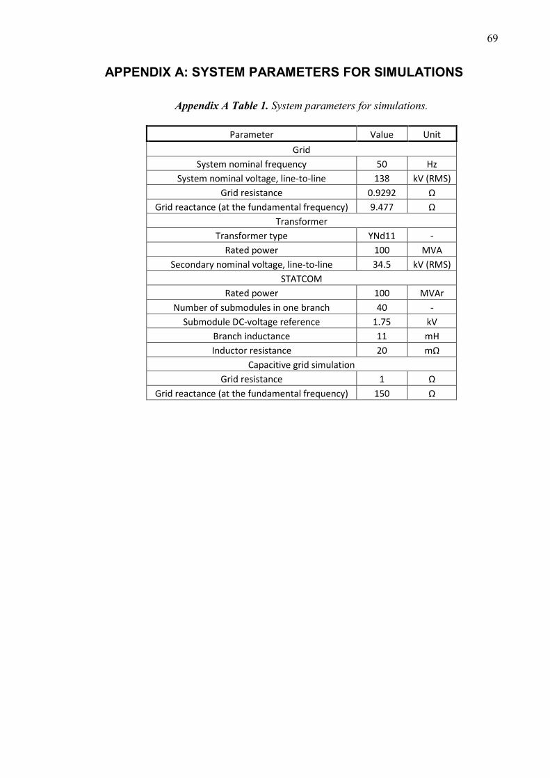
APPENDIX A: SYSTEM PARAMETERS FOR SIMULATIONS
Page 7
vi
LIST OF SYMBOLS AND ABBREVIATIONS
AC Alternating Current
DC Direct Current
DDSRF Decoupled Double Synchronous Reference Frame
DSOGI Double Second Order Generalized Integrator
FACTS Flexible AC Transmission Systems
FLL Frequency Locked Loop
GTO Gate Turn-Off Thyristor
HVDC High Voltage Direct Current
IGBT Insulated Gate Bipolar Transistor
MDSOGI Multiple Double Second Order Generalized Integrator
MMC Modular Multilevel Converter
MSOGI Multiple Second Order Generalized Integrator
PCC Point of Common Coupling
PLL Phase Locked Loop
PNSC Positive Negative Sequence Calculator
PWM Pulse Width Modulation
SOGI Second Order Generalized Integrator
SRF Synchronous Reference Frame
SVC Static Var Compensator
STATCOM Static Synchronous Compensator
THD Total harmonic distortion
VSC Voltage Source Converter
a A phase shift of 120 degrees
D Distortion power
h Order of the harmonic component
I1 Fundamental current RMS value
Ih Current harmonic component h RMS value
IP Active current
IQ Reactive current
k SOGI gain
kc Active power capacity increase factor
kPV Losses reduction factor
n Number of submodules in series
P Active power
Pa Losses due to active power
Pr Losses due to reactive power
Pl Thermal power losses
Q Reactive power
q 90 degrees phase shift
qv’ SOGI’s inquadrature output signal
R Resistance
S Apparent power
U Magnitude of the voltage vector in synchronous reference frame
Ud Pure DC component of the voltage d component
Uq Pure DC component of the voltage q component
v Instantaneous voltage signal
v’ SOGI’s instantaneous output voltage
Page 8
vii
V1 Fundamental voltage RMS value
vabc A three-phase voltage vector in natural reference frame
vαβ Voltage vector in αβ-frame
vαβ,rotated Rotated voltage vector in αβ-frame
Va Phase A voltage phasor
VAB1 Primary side line-to-line voltage between phases A and B
Vab1 Secondary side line-to-line voltage between phases A and B
VAN1 Primary side phase A voltage
Vb Phase B voltage phasor
VBC1 Primary side line-to-line voltage between phases B and C
Vbc1 Secondary side line-to-line voltage between phases B and C
VBN1 Primary side phase B voltage
Vc Phase C voltage phasor
VCA1 Primary side line-to-line voltage between phases C and A
Vca1 Secondary side line-to-line voltage between phases C and A
VCN1 Primary side phase C voltage
vd Voltage d component
vdh Harmonic oscillation in voltage d component
vdq Voltage vector in synchronous reference frame
VGRID Grid voltage
Vh Voltage harmonic component h RMS value
VLL Line-to-line voltage
Vn1 Voltage at the sending end
Vn2 Voltage at the receiving end
VPCC Voltage at the point of common coupling
vq Voltage q component
vqh Harmonic oscillation in voltage q component
VVSC Voltage produced by VSC
X Reactance
XL Line reactance
ZGRID Grid impedance
γ FLL gain
δ Phase difference between Vn1 and Vn2
εf Frequency error variable
εv SOGI’s error signal
θ Rotation angle
θsync Synchronization angle
φ Initial angle of the voltage vector
φa Initial power factor angle
φb Final power factor angle
φ1 Phase difference between voltage and current waveforms
ω Angular frequency
ω’ SOGI’s resonance frequency
ωf Cut-off frequency of the low-pass filter
ωff FLL feedforward
ωsync PLL angular synchronization frequency
Page 9
1
1. INTRODUCTION
The increasing use of power electronic devices and other nonlinear loads has thrown a
tremendous challenge for power system operators to maintain the good power quality in
power systems [1]. Harmonic currents and voltages injected by these nonlinear loads in-
crease losses, decrease the overall system performance and can have a harmful impact on
the entire system if not addressed properly. Due to this, it has become necessary to limit
these harmonics’ impacts by compensating substantial grid harmonics. Consequently,
various standards have been published to limit the level of distortion in power systems.
To reduce the harmonic content in power systems, several harmonics mitigation tech-
niques have been developed. A traditional method to solve the problem of harmonic pol-
lution has been to install passive power filters, consisting of tuned circuits of passive
components such as inductors and capacitors, to absorb harmonic currents from the grid.
However, these passive power filters have a number of shortcomings especially under
changing grid conditions. As a result, more complex techniques have been designed to
respond better to harmonic standards as well as enabling better adaptation to project spe-
cific requirements. Active power filters represent newer technology in the field of har-
monics mitigation. [2]
As the electricity demand continues to grow, reactive power compensation has become
more and more important by enabling maximization of the active power transmission
capacity of the grid. Static Synchronous Compensator (STATCOM) is a modern reactive
power compensation solution consisting of a voltage source converter, reactor and a step-
down transformer. [3] The purpose of this thesis is to study possibilities for active har-
monic filtering as an add-on feature on a Modular Multilevel Converter (MMC) based
STATCOM system. Active harmonic filters done by two-level and three-level topologies
on low voltage application are common but active harmonic filters on high voltage side
can be considered a more novel example of active filtering [2, 4]. Correspondingly, re-
gardless of the number of works published concerning MMC in the fields of Flexible AC
Transmission Systems (FACTS) and High Voltage Direct Current (HVDC), the operation
of MMC as an active power filter in high voltage applications isn’t well-covered. [4] In
this thesis, two harmonics detection methods are studied and compared comprehensively.
Moreover, their feasibilities in harmonics compensation as a part of the normal operation
of a full-scale MMC STATCOM are further simulated in PSCAD environment.
In chapter 2, basic theory of harmonics, their effects and a review of harmonic standards
are presented. In chapter 3, fundamentals of reactive power compensation are described.
Moreover, the structure and operation principle of the MMC based STATCOM system
Page 10
2
are presented. The chosen harmonics detection methods with grid synchronization fea-
tures are presented in chapter 4 which thus can be considered as the core chapter of this
thesis. In chapter 5, the studied techniques are simulated in PSCAD environment to
demonstrate their feasibilities. Chapter 6 provides an analysis and comparison of the stud-
ied two methods based mainly on chapters 4 and 5. Chapter 7 proposes possible future
study needs to further develop the active harmonic filter feature. Finally, the last chapter
sums up the entire thesis and provides final conclusions from the results.
Page 11
3
2. HARMONICS
Harmonic distortion is one of the most important issues in today’s power systems. In this
chapter, the basic theory and phenomena related to power system harmonics are pre-
sented. Moreover, in the last subchapter important standards defining allowed harmonic
distortion levels are presented briefly.
2.1 Basics of harmonic theory
In an ideal case, a power system consists of ideal power generators and linear loads. Un-
der these circumstances, currents and voltages will be in shape of an ideal sine wave with
a specified voltage magnitude and a constant frequency. However, for a number of rea-
sons these conditions are not fulfilled in practice which leads to distorted current and
voltage waveforms often expressed as harmonic distortion.
A linear load in an electric power system draws current which is proportional to the ap-
plied voltage. Hence the voltage waveform equals to the current waveform. Typical linear
loads are for example heaters, incandescent lamps and motors. In turn, on a nonlinear
load the shape of current waveform is not the same with the voltage waveform. Imped-
ance of a nonlinear load changes with the applied voltage resulting in non-sinusoidal cur-
rent drawn by the load. [5] Standard IEEE 519 defines nonlinear load as a load that draws
a non-sinusoidal current wave when supplied by a sinusoidal voltage source [6]. Nonlin-
ear loads thus lead to harmonic distortion. Rectifiers, adjustable speed motor drives and
ferromagnetic devices are typical examples of nonlinear loads.
According to Fourier theorem, all non-sinusoidal periodic signals can be represented as a
sum of simple sinewaves [7]. Regardless of how complex the signal is, when analyzed
through the Fourier series analysis it is possible to deconstruct the signal into a series of
simple sinusoids. This means that even highly distorted currents and voltages of the power
system can be decomposed of the fundamental signal and possibly an infinite set of si-
nusoidal terms whose frequencies are integer multiplies of the fundamental frequency.
These multiplies are called harmonics. Figure 1 shows a distorted total current and its
decomposition.
Page 12
4
Figure 1. Distorted waveform decomposed into fundamental signal and harmonics.
As can be seen in Figure 1, the distorted total current is composed of the fundamental
frequency current and harmonic currents of 3rd, 5th and 7th order. According to standard
IEEE 519 a harmonic can be defined as a sinusoidal component of a periodic wave or
quantity having a frequency that is an integral multiple of the fundamental frequency [6].
Devices causing harmonics are present in all industrial, commercial and residential in-
stallations. The problem of distorted waveforms in power systems is thus not a new phe-
nomenon. However, the increasing number of highly nonlinear loads such as power elec-
tronic devices have created a growing concern for this issue nowadays.
2.2 Sources of harmonics
There exist plenty of harmonics sources especially in industrial power systems. A com-
mon characteristic for all these sources is a nonlinear voltage-current operating relation-
ship. Any device that alters the pure sinusoidal waveform of currents or voltages is con-
sidered as a harmonic source.
Ideally, an AC generator produces pure sinusoidal voltage waveform at a fundamental
frequency without any harmonics. This is the case only if generator’s structure and oper-
ation are theoretically perfect i.e. windings are evenly and finely distributed and magnetic
field is uniform. However, generators are not ideal in practice but have many flaws which
result in non-sinusoidal voltage generation and thus harmonics supply to the grid. For
example, variation in generator’s airgap, non-ideal winding types and asymmetrical struc-
ture overall induce voltage distortion. This distortion level at the supply end is not signif-
icant but it still exists. In other words, harmonics are there even if all loads were linear
and ideal. [8]
Page 13
5
Nowadays, there exist numerous different situations where harmonics are generated. The
greatest majority of harmonic sources can be considered to origin from power converters
that use solid-state switching devices. These are for example rectifiers, inverters, voltage
controllers, frequency converters and variable frequency drives. Overall nowadays in-
creasing use of power semiconductor devices create waveforms rich in harmonics. Power
converters, transformers and rotating machines can be considered as traditional sources
of harmonics. Other fundamental harmonics sources are for example arc-furnaces, fluo-
rescent lightning and other network’s nonlinear loads. [1, 7]
In the future the issue of harmonics will be even more challenging as the harmonic sources
will become diverse and more numerous. Especially the use of distributed generation
(photovoltaics and wind power) is estimated to play a significant role in power generation
in the future and will thus create challenges concerning power system harmonics. Also,
the potential large-scale use of electric vehicles, which draw a significant amount of en-
ergy when charged, can significantly increase harmonics generation. Moreover, the in-
creasing use of sensitive electronics will worsen the situation. [1, 7]
2.3 Effects of harmonics
The effects of harmonics distortion on different equipment vary extensively. Different
machines and equipment respond differently to harmonics incidence depending on the
characteristics of the equipment and the method of operation. For instance, conventional
electric heating machines, stoves and incandescent lamps are basically immune to any
harmonics distortion. On the other hand, in many cases harmonics may cause shortening
of lifetime, increased losses and even malfunctioning in some electronic devices.
One of the main problems with harmonics is simply increased current in the system. Un-
wanted distortion can increase conductor’s current resulting in increase of thermal losses
and in the worst-case tripping of protection. Nowadays, operation of various devices de-
pends on accurate magnitude and shape of the voltage waveform. Harmonics lead to in-
correct magnitude values and distorted wave shape, which therefore may cause malfunc-
tioning of equipment. For example, some measuring and protective instruments are prone
to error under harmonics influence. [9] Moreover, possible parallel or series resonance in
the system can cause amplification of harmonics and thus lead to even more problematic
conditions for electric devices. In general, higher harmonics force the system to operate
outside its normal specifications, which naturally leads to higher energy consumption and
challenges in maintaining the normal operation. [10]
Since harmonics are of higher frequency compared to the fundamental component they
tend to avoid flowing through the center of a solid conductor. In other words, they flow
mainly near the conductor’s surface thus reducing the effective cross-sectional area of the
conductor. This leads to lower conductivity and higher losses since conductor’s cross-
Page 14
6
sectional area available to carry electron flow is not used effectively. As a result, harmon-
ics flow between the outer edge and so-called skin depth. The higher the frequency of a
harmonic is, the smaller the skin depth and thus the greater resistance of the conductor,
respectively. [11] This phenomenon is known as skin effect and it can be considered as a
substantial issue increasing losses in many applications.
In addition to earlier, increased eddy current losses due to harmonics are a major issue
especially when considering for example transformers and motors. Whereas copper losses
are directly proportional to the resistance and the square of the load current, eddy current
losses are directly proportional to the square of the product of current and its correspond-
ing frequency. Increased losses due to skin effect and higher eddy current losses may
together lead to overheating of windings in motors and transformers, cause thermal insu-
lation loss due to heating and thus lead to premature ageing and reduction in performance.
[7, 10, 12]
In a four-wire three-phase system harmonic currents may have a significant impact on the
neutral conductor. Under normal conditions, balanced phase currents cancel out each
other in the neutral conductor i.e. there is no current flowing through the neutral. How-
ever, when the system is not entirely balanced, unbalanced currents circulate through the
neutral conductor. Moreover, under highly distorted circumstances harmonics zero se-
quence currents add in phase in the neutral conductor. The circulation of these zero se-
quence harmonics in addition to the circulation of the fundamental frequency unbalanced
currents may lead to neutral conductor overloading. As the neutral conductor is usually
sized the same as phase conductors, dangerous overheating may occur. [1]
Overall, harmonics can have numerous harmful impacts which generally can be catego-
rized into long-term and short-term effects. Long-term effects are mainly of thermal na-
ture whereas short-term effects are failures and malfunctions of devices. Harmonics can
furthermore go unnoticed for long periods of time if not detected properly. If harmonics
are not controlled appropriately they can for example increase temperatures, lead to re-
duction in equipment’s service life, cause damage to parts of the entire power system and
thus create additional costs for the power system operator.
2.4 Harmonics analysis and THD
Harmonics analysis can be carried out in frequency domain instead of presenting current
and voltage harmonics in time domain. The frequency domain presentation shows how
much of the original signal lies within each given frequency band over a range of fre-
quencies. The time domain representation in turn shows how the signal varies within time
and gives thus more information about the real-time characteristics of the signal. As men-
tioned earlier, with Fourier’s transform signals can be converted from time domain to
frequency domain. Usually the outcome is presented in a bar chart as shown in Figure 2.
Page 15
7
Figure 2. Distorted current waveform presented in a bar chart.
Figure 2 presents the same current waves in a bar chart as were presented earlier in time
domain in Figure 1. The first bar presents the fundamental frequency and the rest of the
bars present harmonics, respectively. As can be seen, in the frequency domain represen-
tation, it can be easily noticed which harmonics occur in the original signal and in what
scale. The analysis of harmonics is preferable to carry out in frequency domain. [1]
Total harmonics level in voltage and current waveforms needs to be estimated. This is
necessary in order to implement proper means to mitigate harmonics in power systems
and to prevent harmonics’ negative influence on power system equipment. Distortion of
a waveform in relation to ideal pure sine wave is analyzed by total harmonic distortion
(THD). The total harmonic distortion is defined as a ratio of a sum of all harmonics com-
ponents to the fundamental component of the signal. [1] For instance, total harmonic dis-
tortion for current is defined as follows:
𝑇𝐻𝐷 = √∑ 𝐼ℎ
2∞ℎ=2
𝐼1 , (1)
where I1 is the fundamental current RMS value and In is the current RMS value of a cor-
responding harmonic order h. For voltage, the total harmonic distortion can be defined
according to equation (2), respectively.
𝑇𝐻𝐷 = √∑ 𝑉ℎ
2∞ℎ=2
𝑉1 (2)
In equation 2, V1 is the fundamental voltage RMS value and Vn the voltage RMS value of
a corresponding harmonic order h analogically to equation 1. In general, the less the par-
ticular signal looks like a pure sine wave, the stronger the harmonic content in it is and
Page 16
8
the greater THD value it has. Therefore, THD should be minimized to maintain the quality
of electricity in electric power systems; ideal pure sine wave has zero distortion level i.e.
THD = 0 %. Lower THD in power systems means higher efficiency, higher power factor
and lower peak currents. Different standards and regulations also define limits for har-
monics distortion under which all harmonics should be kept. [1]
2.5 Harmonics mitigation methods
As mentioned earlier, electrical harmonic pollution is necessary to be minimized in order
to keep electric networks and the whole power system safe and efficient. Harmonics can
be filtered with different components and techniques of which the most important ones
are passive and active filters.
Passive filters consist of passive components such as capacitors, inductors and resistors.
Tuning of the filters are done by combining these passive components thus allowing fil-
ters with specific characteristics. Passive filters can be connected either in series or in
parallel with the load. The existing harmonic filtering is nearly entirely based on parallel
type of filters and although series configuration is also possible it is more common to
connect passive filters in parallel. [13] The main idea of parallel passive filters is to create
a low-impedance path from the electric network to ground for a predefined harmonic
signal. This way the harmonic passes to the ground through the passive filter and does
not spread to the rest of the electric network. Passive filters have a special frequency
where the impedance of the filter approaches zero or respectively infinity in case of series
type of passive filters. This frequency is known as resonance frequency. Designing of the
filter is done so that its resonance frequency meets the frequency of a predefined har-
monic. Thus, for parallel connected filters, the filter is tuned in a way that its impedance
approaches zero around the harmonic frequency. In contrast, with series type of passive
filters, the filter should present high impedance for the predefined harmonic frequency
that needs to be blocked. [2]
The main drawback with passive filters is that they are capable of filtering only predefined
harmonics. Also, if harmonic’s characteristics vary, for example frequency fluctuates, the
passive filter is immediately detuned and can’t filter out the specific harmonic efficiently
anymore. In other words, if filters were capable to automatically correct tuning due to
varying characteristics such as frequency variation and component deviation, a significant
advantage would be obtained. [13] Active filters are the solution for this issue since they
can filter several harmonics and continuously adjust tuning to cancel out varying harmon-
ics. Similar with passive filters, active filters can also be connected either in parallel or in
series. Thus, they are categorized into shunt active filters and series active filters based
on their circuit configurations. However, as it was with passive filters also shunt type of
active filters are more common over series type of active filters. The main idea of active
filters is to produce a waveform to the grid with the same magnitude but with 180 degrees
shifted phase compared to the detected harmonic signal. Thus, the harmonic in the grid
Page 17
9
will be canceled out. In order to work properly, active filters need to detect harmonic’s
frequency, magnitude and phase in the grid. After detecting the harmonic, active filters
sync and inject the created waveform with opposite phase angle to the grid so that the
original grid harmonic will finally be canceled out. Active filters have many advantages
compared to traditional passive filters but so far the cost has still been higher. [2, 13]
2.6 Regulations and standards
There are several different standards and regulations defined regarding harmonic pollu-
tion in power systems. The purpose of these regulations is to ensure proper operation of
the network and connected equipment by preventing harmonic distortion to exceed per-
missible levels. According to standard IEEE 519 harmonic distortion limits are provided
to reduce the potential negative effects on user and system equipment [6]. Overall these
standards determine the compatibility between distribution networks and connected de-
vices. The main idea is that the harmonics caused by a device must not disturb the distri-
bution networks and on the other hand each device must be capable of operating normally
in the presence of disturbances up to a specific level. There are both international stand-
ards such as IEEE 519 and IEC 61000-2-4 as well as national standards for example G5/3
and G5/4 for United Kingdom. [14] In addition to these international and national stand-
ards, there may also be project-specific limits for harmonics generation and harmonics
effects.
Currently, most of the countries use limits for harmonics based on international standards.
Widely recognized international standards are for example IEEE 519, IEC 61000-3-6,
IEC 61000-2-2, IEC 61000-2-12 and the European standard EN 50160. As not only the
existence of different harmonic components but also the combination of these harmonics
matters, these standards usually give harmonics limits in terms of individual harmonic
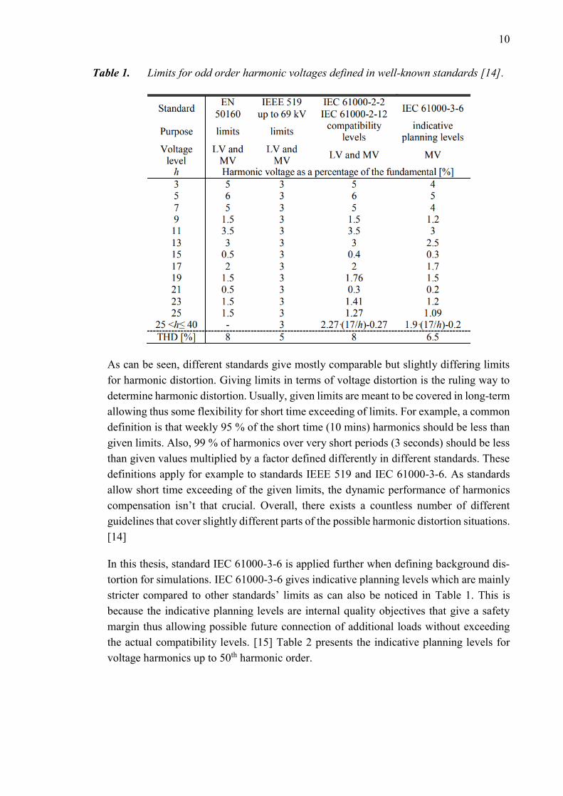
component values but also as total harmonic distortion. Table 1 gives a comparison of
different limits defined in above mentioned standards. The limits are given only for the
odd harmonic orders.
Page 18
10
Table 1. Limits for odd order harmonic voltages defined in well-known standards [14].
As can be seen, different standards give mostly comparable but slightly differing limits
for harmonic distortion. Giving limits in terms of voltage distortion is the ruling way to
determine harmonic distortion. Usually, given limits are meant to be covered in long-term
allowing thus some flexibility for short time exceeding of limits. For example, a common
definition is that weekly 95 % of the short time (10 mins) harmonics should be less than
given limits. Also, 99 % of harmonics over very short periods (3 seconds) should be less
than given values multiplied by a factor defined differently in different standards. These
definitions apply for example to standards IEEE 519 and IEC 61000-3-6. As standards
allow short time exceeding of the given limits, the dynamic performance of harmonics
compensation isn’t that crucial. Overall, there exists a countless number of different
guidelines that cover slightly different parts of the possible harmonic distortion situations.
[14]
In this thesis, standard IEC 61000-3-6 is applied further when defining background dis-
tortion for simulations. IEC 61000-3-6 gives indicative planning levels which are mainly
stricter compared to other standards’ limits as can also be noticed in Table 1. This is
because the indicative planning levels are internal quality objectives that give a safety
margin thus allowing possible future connection of additional loads without exceeding
the actual compatibility levels. [15] Table 2 presents the indicative planning levels for
voltage harmonics up to 50th harmonic order.
Page 19
11
Table 2. IEC 61000-3-6 indicative voltage harmonic planning levels. Table adapted from
table in [15].
Odd harmonics non-multiple of 3
Odd harmonics multiple of 3 Even harmonics
Harmonic order h
Harmonic voltage %
Harmonic order h
Harmonic voltage %
Harmonic order h
Harmonic voltage %
5 2 3 2 2 1.4
7 2 9 1 4 0.8
11 1.5 15 0.3 6 0.4
13 1.5 21 0.2 8 0.4
17 ≤ h ≤ 49 1.2∙17/h 21 < h ≤ 45 0.2 10 ≤ h ≤ 50 0.19∙10/h+0.16
The indicative voltage harmonic planning levels given in Table 2 are for high voltage and
extra-high voltage systems (> 35 kV) whereas in Table 1 the values are given for medium
voltage systems. Therefore, limits defined by IEC 61000-3-6 in Table 1 and Table 2 are
different. The voltage THD limit for high voltage systems is 3 % instead of 6.5 % that is
defined for medium voltage system in Table 1. [15] In this thesis, IEC 61000-3-6 for high
voltage systems is applied.
Page 20
12
3. REACTIVE POWER COMPENSATION
Reactive power compensation has become increasingly important as it affects the opera-
tional, economical and quality of the service aspects in electric power systems. In this
chapter, basics of reactive power compensation are presented. Moreover, the last sub-
chapter presents the main structure and operation principle of the STATCOM system in
which the active harmonic filtering is to be implemented.
3.1 Need for reactive power compensation
Active, reactive and apparent powers are fundamental concepts regarding classical single-
phase and three-phase AC systems. In a linear system, current and voltage are both sinus-
oidal and in the same phase if the load is purely resistive. The product of current and
voltage is thus always positive resulting in positive power. This means that energy is
transferred from source to load and furthermore the flow is unidirectional. This power is
useful power and often referred as real power or active power P. On the other hand, if the
load is purely reactive, i.e. capacitive or inductive, the phase difference φ1 between volt-
age and current is 90 degrees and thus the product of current and voltage is positive during
two quarters and negative during the other two quarters of the cycle. This means that
energy transferred to the load is as much as energy coming back from the load. In other
words, energy flows back and forth between the source and the load resulting in zero
average power. [16] This power is often referred as reactive power Q. Calculations of
active and reactive powers as well as their relationship to apparent power S are presented
in equations 3–5.
𝑃 = 𝑉 𝐼𝑐𝑜𝑠 𝜑1 (3)
𝑄 = 𝑉𝐼 𝑠𝑖𝑛 𝜑1 (4)
𝑆 = √𝑃2 + 𝑄2 (5)
In equations 3–5, V is the RMS phase voltage, I is the RMS current of one phase and φ1
is the phase difference between the phase voltage and current. The calculated powers are
single-phase powers. Usually, these powers are calculated from fundamental voltage and
current values. If harmonics are present, their effect can be expressed with the help of an
additional power called distortion power D. Moreover, the ratio of active power P to ap-
parent power S is referred as power factor cosφ1 which is considered as an important
power quality measure. Power factor equals one when all the power is active power and
zero when all the power is reactive power, respectively.
All real equipment in the power system either generate or consume reactive power and
both active and reactive powers are needed for the electric network to function properly.
Page 21
13
In practice, reactive power naturally increases losses as energy travelling between the
source and the load loses its energy due to for example line resistances. Reactive power
would therefore be beneficial to be created near the load where needed rather than draw-
ing it through the grid.
One of the main issues with the transmission of reactive power is the increased current
and thus increased thermal losses along transmission and distribution lines. The power
losses due to line impedance are proportional to the square of the line current and are
determined in a three-phase system as follows:
𝑃𝑙 = 3 𝐼2𝑅, (6)
where R is resistance of the conductor and I is the line current. By reducing reactive power
transfer, smaller currents flow through the lines and thus thermal losses can be reduced
radically. [17] To further illustrate the importance of the reactive power compensation,
the relationship between thermal losses and the power factor cosφ1 can be derived as
shown in the following equation:
𝑃𝑙 = 3 𝐼2𝑅 =𝑆2𝑅
𝑉𝐿𝐿2 =
𝑃2𝑅
𝑉𝐿𝐿2 ∙(𝑐𝑜𝑠 𝜑1)2 =
𝑃2𝑅
𝑉𝐿𝐿2 +
𝑄2𝑅
𝑉𝐿𝐿2 , (7)
where R is the resistance of the network component for example resistance of the con-
ductor, I, S, P and Q are the current, total power, active power and reactive power flowing
through the network component, VLL is line-to-line voltage and cosφ1 is the power factor.
As can be seen, losses are inversely proportional to the square of the power factor cosφ1.
If power factor is improved from cosφa to cosφb losses are reduced in turn by a factor of
kPV.
𝑘𝑃𝑉 = 1 − (𝑐𝑜𝑠 𝜑𝑎
𝑐𝑜𝑠 𝜑𝑏 )
2
(8)
In equation 7, this relationship is further derived into form where active power part and
reactive power part of the losses are easily found. Figure 3 illustrates the relationship
between losses and the power factor.
Page 22
14
Figure 3. Relationship between power factor and the ratio of losses caused by reactive
power flow to losses caused by active power flow [18].
In Figure 3, Pr represents losses due to reactive power flow and Pa losses due to active
power flow, respectively. It can be noticed that the power factor reaches the unity value
only if the part of losses due to reactive power flow becomes zero. Improved power factor
can result in optional use of smaller cross-sectional area of line conductors, less thermal
insulation and thus smaller investments when constructing transmission and distribution
lines. [17, 18]
Different standards define requirements for voltage quality and for permissible voltages
in power systems. For example, standard EN 50160 specifies the main characteristics of
the electricity supplied by public low, medium and high voltage AC electricity networks
[19]. Standard IEC 60038 defines moreover standard voltages in power systems and fur-
ther permissible voltage drops for different standardized voltage levels [20]. As the volt-
age needs to be kept at a specific level in the electricity network to fill the power quality
requirements set by standards and further specifications, voltage drops across network
components must be estimated. This can be calculated with the following equation:
∆𝑉 = 𝑃𝑅+𝑄𝑋
𝑉=
𝑃𝑅
𝑉(1 +
𝑄𝑋
𝑃𝑅), (9)
where X is the reactance of the network component. As can be seen, the voltage drop is
dependent on both the ratio of reactive power and active power Q/P and the ratio of reac-
tance and resistance X/R. To minimize the voltage drop V the ratio of reactive power to
active power should be minimized. The greater the ratio of reactance to resistance is the
greater effect is seen in reduction of voltage drop when the ratio Q/P is minimized. [18]
To meet voltage quality requirements and voltage drop limits, conductors with large
enough cross-sectional area must be chosen when building new electricity transmission
and distribution lines. Correspondingly, the increasing use of electricity and thus a need
to transfer more and more power through the same power lines leads to a need for
strengthening or renewing of old transmission lines. However, by reducing reactive
Page 23
15
power transferred through transmission lines by reactive power compensation it is possi-
ble to increase active power transmission capacity of the existing lines without making
investments to strengthen or rebuild them. The active power transfer capacity of an exist-
ing transmission line can be increased by a factor of kc, as shown in equation 10, if the
power factor is improved from cosφa to cosφb.
𝑘𝑐 = (𝑐𝑜𝑠 𝜑𝑏
𝑐𝑜𝑠 𝜑𝑎) (10)
Reactive power compensation can reduce the losses along the entire power system and
on the other hand make it possible to transfer more active power with the same transmis-
sion lines. [17, 18]
Overall, the transmission of reactive power in power systems has numerous disadvantages
such as an increase of thermal losses and voltage drops, active power transfer capacity
reduction and consequently increased costs of electricity supply. However, reactive
power compensation can improve the performance of the whole power system and after
all reduce operational costs and costs for investments.
3.2 Compensation methods
Reactive power is generated because of reactive loads as noted earlier. In a simple form,
depending on whether the load is inductive or capacitive the reactive power component
can be compensated by adding either capacitive or inductive component to the grid. This
way the original reactive power component will be canceled out as far as the added com-
pensation component is correctly rated. There are several different ways to implement
reactive power compensation but overall all compensation methods can be divided into
two categories: shunt connected and series connected compensators.
3.2.1 Shunt compensation
Usually, a load requires reactive power and draws it from the grid. In other words, a
source must provide this reactive power to the grid, which increases line current as noted
earlier. The main principle of shunt compensation is to provide this reactive power near
the load in which case reactive power is not needed to be transferred from the source
through power lines.
Figure 4 illustrates a system consisting of a voltage source, an inductive load and a power
line. Moreover, it shows system’s phasor diagram in a case without reactive power com-
pensation.
Page 24
16
Figure 4. Power system and its phasor diagram without reactive power compensation
[21].
Current drawn by the load consists of active current IP and reactive current IQ. In shunt
compensation, the reactive part of the current is produced near the load resulting in only
active power to be transferred through power lines. Figure 5 shows the same system and
its phasor diagram in a case when reactive power compensation is done with a current
source.
Figure 5. Shunt compensation with a current source [21].
As can be seen, the current source produces all the reactive power needed for the load and
thus smaller current flows along power lines transferring only active power from the
source to the load. [21]
Depending on the case, reactive power compensation by shunt compensators can be done
with a capacitor, an inductor, a current source or a voltage source. Traditionally typical
loads in electricity network have been inductive as electric motors, transformers and coils
are inductive by nature. For this reason, a traditional way to carry out reactive power
compensation has been adding capacitor banks to the grid near these inductive loads.
Page 25
17
These capacitor banks provide the reactive power needed by inductive loads. More ad-
vanced shunt type of reactive power compensation can be done for example with Static
Var Compensator (SVC) or Static Synchronous Compensator (STATCOM). [21]
3.2.2 Series compensation
Reactive power compensation can also be done with a series compensation system. A
common case is to install a series capacitor on a transmission line. Correctly rated capac-
itor decreases the total reactance of the transmission line resulting in improved perfor-
mance of the power transfer. The active power transfer over a line can be expressed as
follows:
𝑃 =𝑉𝑛1𝑉𝑛2
𝑋𝐿𝑠𝑖𝑛 𝛿, (11)
where Vn1 is the voltage at the sending end, Vn2 the voltage at the receiving end and δ is
the phase angle between Vn1 and Vn2. In other words, if a capacitor having a reactance XC
is connected in series with the line, the reactance of the line is reduced from XL to XL-XC.
As a result, the active power transfer capacity can be increased. The series capacitor may
be located at the sending end, receiving end or at the center of the line. [21]
Series compensation can theoretically be also implemented for example with a voltage
source. Figure 6 illustrates the same system as earlier but now the compensation is done
with a series type of voltage source installed between a load and the power line.
Figure 6. Series compensation with a voltage source [21].
As can be seen in Figure 6, when correctly adjusted the voltage source compensator pro-
duces its voltage in a way that as a result only active power flows between the source and
V2. However, the most common solution for series compensation is to use series capaci-
tors as mentioned earlier. [21]
Page 26
18
3.3 STATCOM
Static Synchronous Compensator (STATCOM) is a shunt connected reactive power com-
pensation device that is capable of generating and absorbing reactive power. It consists
of a controllable, power electronic switches based, voltage-source converter (VSC) which
is located behind a coupling reactor. STATCOM can be seen as a solid-state switching
converter feeding its output from an energy storage device at its input terminals. STAT-
COM produces its output based on DC voltage which it modulates according to the ref-
erence so that a desired current is achieved with the help of voltage over its coupling
reactor. In other words, it provides the wanted reactive power generation and absorption
completely through electronic processing of the voltage and current waveforms in a volt-
age-source converter. STATCOM’s one main advantage is that its reactive power com-
pensation capability is not dependent on the grid voltage which thus makes it possible to
provide the maximum rated inductive and capacitive current independent of the grid volt-
age. In other words, by not relying on passive components to produce reactive power, like
extensively used conventional Static Var Compensator (SVC) does, STATCOM’s un-
dervoltage performance is far greater than SVC’s. Moreover, compared to SVC, STAT-
COM has better dynamic performance, faster response and smaller size (footprint) but
with a cost of higher price. [3]
3.3.1 Structure and operation principle
STATCOM consists of a controllable voltage-source converter (VSC), a coupling reactor
and a coupling or a step-down transformer. The voltage-source converter is a DC to AC
converter operated from an energy storage capacitor. STATCOM’s basic configuration is
presented in Figure 7.
Figure 7. STATCOM’s basic configuration [3].
To illustrate the basic principle of STATCOM’s reactive power generation a simplified
equivalent circuit is presented in Figure 8.
Page 27
19
Figure 8. Simple equivalent circuit of STATCOM.
The equivalent circuit consists of an ideal voltage source VGRID as grid voltage, which is
reduced to the transformer secondary side, Voltage Source Converter VVSC and a reac-
tance X which is a sum of coupling coil and transformer reactances. The reactive power
of STATCOM depends on the voltage across the reactance X. In other words, reactive
current IQ drawn by STATCOM depends on the voltage magnitude difference between
VSC produced VVSC and the grid voltage VGRID. If losses are not considered, VSC pro-
duces a three-phase voltage VVSC in phase with the three-phase voltage VGRID of the sys-
tem. Thus, according to the basic circuit theory, reactive current IQ can be formed with
the help of VGRID, X and VVSC as presented in equation 12.
𝐼𝑄 =𝑉𝐺𝑅𝐼𝐷−𝑉𝑉𝑆𝐶
𝑋 (12)
As a result, the corresponding reactive power Q drawn from the grid can be expressed as
follows:
𝑄 = 𝑉𝐺𝑅𝐼𝐷𝐼𝑄 =1−
𝑉𝑉𝑆𝐶𝑉𝐺𝑅𝐼𝐷
𝑋𝑉𝐺𝑅𝐼𝐷
2 (13)
On the basis of above equation 13, by controlling the voltage magnitude of the VSC the
reactive power flow can also be controlled. If the produced VVSC is greater than VGRID a
leading current is produced resulting in capacitive power generated by STATCOM. Re-
spectively, if the grid voltage VGRID is greater, the resulting current lags the grid voltage
and thus reactive power is absorbed. In other words, by varying VSC’s output voltage
magnitude, the reactive power flow between STATCOM and the grid can be controlled.
To clarify different operation schemes phasor diagrams are presented in Figure 9.
Page 28
20
Figure 9. Phasor diagrams for A) capacitive power and B) inductive power operation
schemes.
Figure 9A) illustrates the capacitive power operation scheme and respectively Figure 9B)
presents the inductive power operation scheme. If the produced VVSC magnitude equals
VGRID, the voltage across reactance X is zero and thus STATCOM operates at its zero-
operation point which means no reactive power flows between the grid and STATCOM.
[3]
In an ideal case, STATCOM would produce sinusoidal output voltage, draw sinusoidal
reactive current and moreover the DC capacitor average current would equal zero. In
practice, due to switching losses and other internal losses the energy stored in the DC
capacitor would discharge if the losses were not compensated. The compensation can be
done by making the produced voltage lag the grid voltage by a small angle which results
in active power being supplied from the grid to cover the internal losses in VSC. This
method is based on equation 11. Hence, the DC capacitor voltage can be kept at a desired
level. Moreover, as the produced voltage is never a perfect sinusoid, harmonics are gen-
erated to the grid. [3]
3.3.2 Switching devices and converter topologies
There are various controllable solid-state switches that can be used in VSCs but only few
are suitable for high power applications. Each switching device has different operating
characteristics as well as strengths and weaknesses in respect to rated power, switching
frequency, switching losses etc. A Gate-Turn-Off thyristor (GTO) and an Insulated Gate
Bipolar Transistor (IGBT) are the most commonly used switches in high power applica-
tions. GTO is a mature technology with higher power ratings whereas IGBT is newer
technology in power electronics with higher switching frequency and speed as well as
lower losses. [22]
Page 29
21
The simplest converter topologies capable of producing AC output from DC input are
two-level and three-level converters where the number of levels refers to possible output
voltage levels. For example, a two-level converter can only produce positive and negative
voltages i.e. simple square-wave whereas a three-level converter can produce positive,
negative and zero outputs. Naturally, the produced voltage waveform with two and three-
level converters is not of the same shape with an ideal sinewave which means a great
number of harmonics being created. In order to reduce the harmonic content in the pro-
duced voltage, the simple three-level converter can be extended to a multi-level converter
thus enabling a production of better sinusoidal waveforms. [22] In other words, with
multi-level converters the switches are controlled in a way to produce a staircase voltage
waveform that approximates a sinusoid. However, the circuit and control complexity in-
creases significantly with the increasing number of voltage levels.
The switching is usually done either according to fundamental switching method or with
Pulse Width Modulation (PWM) method. In fundamental switching method switching is
done once in a fundamental cycle which results in a great number of harmonics occurring
in the output voltage. On the other hand, with PWM method the switching can be done
multiple times in one cycle which thus reduces harmonics created similar with the multi-
level converter topology. However, as switching times increase with PWM method, nat-
urally also more switching losses are generated. [22]
3.3.3 Studied STATCOM
In this thesis, Modular Multilevel Converter (MMC) based STATCOM is studied. MMC
is a type of a multi-level converter that consists of multiple submodules connected in
series. Each submodule consists of four IGBT switches that have antiparallel-connected
diodes. In other words, each submodule has so called full-bridge topology that can pro-
duce three output voltage levels thus making one submodule act as a three-level converter
topology. The total voltage of one phase is formed as a sum of individual submodule
voltages consequently making it possible to produce 2n+1 voltage levels, where n corre-
sponds to the number of submodules in series.
The series-connected submodule structure in one phase is called a branch. In this thesis,
a three-phase converter topology is achieved by connecting the three branches in delta
(delta-connected STATCOM). Moreover, a wye-delta connected step-down transformer
is used to connect STATCOM to the grid. These delta connections affect voltage and
current positive and negative sequence components differently which needs to be consid-
ered when implementing the active filter feature.
Page 30
22
4. HARMONICS DETECTION METHODS AND GRID
SYNCHRONIZATION
Detection methods used for harmonics compensation can be generally categorized into
frequency domain methods and time domain methods. In this chapter, two time domain
based methods, a Second Order Generalized Integrator based method and a synchronous
reference frame based method, are studied. The basic theory and operation principles of
these two methods are presented and their suitabilities to be used in the studied STAT-
COM system are considered.
4.1 Second Order Generalized Integrator
A concept for a voltage positive sequence component detection by Second Order Gener-
alized Integrator (SOGI) was originally presented by P. Rodriguez in [23]. This method
is since further developed to suit for harmonics detection and compensation as a fre-
quency adaptive filter. SOGI has similarities for example with a Proportional-Resonant -
controller (PR-controller) structure where generalized integrator part is also introduced.
Figure 10 presents the structure of the SOGI.
Figure 10. Structure of a single SOGI [23].
In Figure 10, v is the instantaneous input voltage signal, v’ and qv’ are two inquadrature
output signals and k and ω’ are referred as SOGI’s gain and resonance frequency, respec-
tively. The output signal v’ is in phase with the input signal v having also the same mag-
nitude whereas the qv’ is in 90 degrees phase shift lagging thus both v and v’. Transfer
functions from input signal v to output signals v’ and qv’ are presented in equations 14
and 15.
𝐷(𝑠) =𝑣′
𝑣=
𝑘𝜔′𝑠
𝑠2+𝑘𝜔’𝑠+𝜔’2 (14)
𝑄(𝑠) =𝑞𝑣′
𝑣=
𝑘𝜔’2
𝑠2+𝑘𝜔’𝑠+𝜔’2 (15)
Page 31
23
In Figure 11, bode diagrams for 𝐷(𝑠) and 𝑄(𝑠) are presented when SOGI gain k is 1.41
and resonance frequency ω’ is set to 314 rad/s.
Figure 11. Bode diagrams for D(s) and Q(s).
As can be noticed in Figure 11, SOGI works as a bandpass filter introducing zero dB gain
and zero phase shift at SOGI’s resonance frequency ω’. Equations 16–19 present gain
and phase shift calculation for 𝐷(𝑠) and 𝑄(𝑠).
|𝐷| = 𝑘𝜔′𝜔
√(𝑘𝜔′𝜔)2+(𝜔′2−𝜔2)2 (16)
∟𝐷 = 𝑡𝑎𝑛−1 (𝜔’2−𝜔2
𝑘𝜔′𝜔) (17)
|𝑄| = 𝜔′
𝜔|𝐷| (18)
∟𝑄 = ∟𝐷 −𝜋
2 (19)
In above equations, ω represents the input signal’s frequency. It can be noticed based on
above equations, as well as from the bode diagrams presented in Figure 11, that qv’ is
always lagging 90 degrees behind v’ independent from resonance frequency ω’ and input
signal v. [23]
Page 32
24
Unlike it is stated in [24], the bandwidth of 𝐷(𝑠) isn’t set only by k completely independ-
ent of the resonance frequency ω’. The bandwidth is actually the product of k and ω’.
However, when the resonance frequency is set then the dynamics of SOGI can be set
exclusively by k. Thus, increasing k corresponds to faster response resulting in also lower
selectivity. On the other hand, by decreasing k, a better selectivity can be achieved with
the cost of slower response. For the fundamental frequency SOGI, a critically-damped
response can be obtained with k equal to √2 [23].
When input signal frequency ω and SOGI’s resonant frequency ω’ are exactly the same,
the output signal’s amplitude follows the input signal’s amplitude. If this is violated, as
is the case often in real life systems, SOGI may lose its tracking accuracy resulting in
incorrect signal detection. This can also be noticed in equations 16–19. In other words, a
constant resonant frequency can only be used when the input signal frequency is known
and has no variation. To make SOGI’s resonant frequency adaptive for input signal fre-
quency variation a Frequency Locked Loop (FLL) is introduced. Figure 12 presents the
structure of SOGI with FLL.
Figure 12. Structure of FLL with SOGI [24].
As can be seen in Figure 12, input signals for FLL are SOGI’s output signal qv’ and error
signal εv. γ in the FLL block is called FLL gain and εf respectively the frequency error
variable. The transfer function for signal εv is presented in 20.
𝐸(𝑠) =𝜀𝑣
𝑣=
𝑠2+𝜔’2
𝑠2+𝑘𝜔’𝑠+𝜔’2 (20)
Signals qv’ and εv are in phase with each other always when SOGI’s resonant frequency
i.e. the output signal of FLL is greater than the input signal frequency. However, when
the frequency of the input signal is greater than the resonant frequency of SOGI, signals
qv’ and εv have 180 degrees phase shift. Bode diagrams in Figure 13 justify this.
Page 33
25
Figure 13. Bode diagrams for FLL E(s) and Q(s).
It can be detected by the product of these two signals whether the resonant frequency of
SOGI needs to be increased or decreased to meet the input signal frequency. The FLL
uses integrator controller with a negative gain γ to find the true input signal frequency. In
other words, εf, the product of qv’ and εv, is negative when the input frequency is greater
than SOGI’s resonant frequency thus increasing the value of FLL’s output signal. Re-
spectively, the product of qv’ and εv is positive when the input frequency is lower than
SOGI’s resonant frequency and decreases therefore the value of FLL’s output signal ω’.
Hence with FLL, SOGI automatically tunes its resonant frequency to its input signal’s
frequency. [24]
The FLL has nonlinear dynamics with changing grid voltage. However, the FLL can be
normalized and thus made as a linearized system independent of grid variables and the
SOGI gain k as derived in [24]. Figure 14 shows the FLL block with the gain normaliza-
tion.
Page 34
26
Figure 14. Structure of normalized FLL with SOGI [24].
The new FLL uses also a feedforward term ωff to speed up the frequency detection as can
be seen in Figure 14.
4.1.1 DSOGI
For three-phase systems SOGI-FLL can be upgraded to Double Second Order General-
ized Integrator (DSOGI) consisting of two individual SOGIs and a single FLL as pre-
sented in [25]. In this case, a three-phase input vector vabc is transformed to a voltage
vector vαβ in αβ stationary reference frame by using the Clarke transformation. The Clarke
transformation is presented in equations 21 and 22.
𝒗𝛼𝛽 = [𝑻𝛼𝛽]𝒗𝑎𝑏𝑐 (21)
[𝑻𝛼𝛽] =2
3[1 −
1
2−
1
2
0√3
2−
√3
2
] (22)
The inverse Clarke transformation can be derived based on equation 22. Amplitude-in-
variant Clarke transformation is used, unlike in [25] where power-invariant transfor-
mation is used, in order to preserve original signal’s amplitude unchanged. In three-phase
systems, the analysis of especially unbalanced grid conditions can be simplified by using
so called symmetrical components. Symmetrical components consist of positive, negative
and zero sequence components. Positive sequence components are equal in magnitude
and have phase shifts of 120 degrees in each phase. The phase sequence is the same as
with the original phase quantities (A-B-C). Negative sequence components are also equal
in magnitude and have the same 120 degrees phase shifts but in a reverse phase sequence
(A-C-B). Zero sequence components, in turn, are equal in magnitude and in phase. [26]
Equation 22 represents the relation between phase voltages and symmetrical components.
[𝑉𝑎
𝑉𝑏
𝑉𝑐
] = [1 1 1
𝑎2 𝑎 1𝑎 𝑎2 1
] [
𝑉𝑎+
𝑉𝑎−
𝑉𝑎0
] (23)
Page 35
27
In equation 23, Va, Vb and Vc are voltage phasors of each phase, a represents a 120 degrees
phase shift and superscripts +, – and 0 represent positive, negative and zero sequence
components. These symmetrical components replace the normal phase quantities in the
analysis of three-phase systems. As a consequence, a division to positive and negative
sequence αβ components in stationary reference frame can be done with the help of
SOGI’s inquadrature output signals as shown in equations 24 and 25.
𝒗𝛼𝛽+ = [𝑻𝛼𝛽]𝑣𝑎𝑏𝑐
+ = [𝑻𝛼𝛽][𝑻+]𝒗𝑎𝑏𝑐 = [𝑻𝛼𝛽][𝑻+][𝑻𝛼𝛽]𝑇
𝒗𝛼𝛽 =1
2[1 −𝑞𝑞 1
] 𝒗𝛼𝛽 (24)
𝒗𝛼𝛽− = [𝑻𝛼𝛽]𝒗𝑎𝑏𝑐
− = [𝑻𝛼𝛽][𝑻−]𝒗𝑎𝑏𝑐 = [𝑻𝛼𝛽][𝑻−][𝑻𝛼𝛽]𝑇
𝒗𝛼𝛽 =1
2[
1 𝑞−𝑞 1
] 𝒗𝛼𝛽 (25)
In above equations, q denotes 𝑒−𝑗𝜋
2 i.e. 90 degrees phase shift. Based on equations 24 and
25 two SOGIs are implemented, one for each vα and vβ component. The structure of
DSOGI-FLL is presented in Figure 15.
Figure 15. DSOGI-FLL with PNSC for positive and negative sequence extraction [25].
DSOGI uses only one FLL that adapts the resonant frequency of both SOGIs to input
signal frequency as can be seen in Figure 15. PNSC, in turn, is the Positive Negative
Sequence Calculator based on equations 24 and 25. Finally, after positive and negative
sequence components for vα and vβ are calculated, the inverse Clarke transformation can
be used to solve instantaneous positive and negative sequence components of the phase
voltages. [25]
Page 36
28
4.1.2 MSOGI
Previously presented structures work with detecting the fundamental component of the
input signal. However, to detect multiple harmonics a structure for Multiple Second Order
Generalized Integrator (MSOGI) or more precisely Multiple Double Second Order Gen-
eralized Integrator (MDSOGI) is introduced. MSOGI uses individual SOGIs tuned at dif-
ferent frequencies to extract the fundamental component and selected harmonics from the
input signal. The structure of MSOGI with FLL is presented in Figure 16.
Figure 16. Multiple SOGIs working in parallel and a cross-feedback network [24].
As can be seen in Figure 16, individual SOGIs tuned at different frequencies work in
parallel in order to extract the fundamental component and selected harmonics from the
input signal. The FLL uses only the SOGI block of the fundamental component to detect
the fundamental frequency which is then multiplied by a harmonic order and forwarded
for each SOGI with the corresponding harmonic order. As can also be seen in Figure 16,
a cross-feedback network can be used to radically enhance the accuracy of the MSOGI
system. This is necessary especially when SOGIs are tuned at frequencies close to each
other as is the case with harmonics detection. In other words, each SOGI’s input signal is
comprised by subtracting all the outputs of other SOGIs from the original input signal.
Thus, in an ideal case each SOGI’s input should in the end only contain the particular
harmonic component or the fundamental one. [25]
Page 37
29
Each SOGI can be replaced with DSOGI to obtain positive-negative sequence tracking in
three-phase systems for selected harmonics. For this use, a Positive Negative Sequence
Calculator can again be used similar with the structure in Figure 15. In three-phase sys-
tems, Clarke transformation can be implemented before the actual cross-feedback net-
work to reduce the number of operations. In this case, only two components, α and β,
need to be brought back to the cross-feedback network in comparison to three components
if done with three-phase signals. [25]
As mentioned, the bandwidth of SOGI is the product of its gain k and resonance frequency
ω’. Furthermore, a critically-damped response for the fundamental SOGI can be achieved
with k equal to √2. Thus, to achieve a critically-damped response for the rest of the SOGIs,
the gain of each SOGI is set by dividing the gain of the fundamental SOGI with the har-
monic order h of the SOGI in question. In this thesis, MSOGI is further studied i.e. used
in simulations.
4.1.3 Phase shift due to delta-connections and grid impedance
In this thesis, in general terms, harmonics compensation is done by measuring the phase
voltages at the point of common coupling (PCC), detecting harmonics with the help of
e.g. MSOGI and by creating a reference current that produces the wanted VSC voltage
and thus the wanted compensation current. As mentioned in chapter 3.3.3 the system
studied is a delta-connected STATCOM behind a star-delta connected stepdown trans-
former. Positive and negative sequence voltages and currents undergo a phase shift when
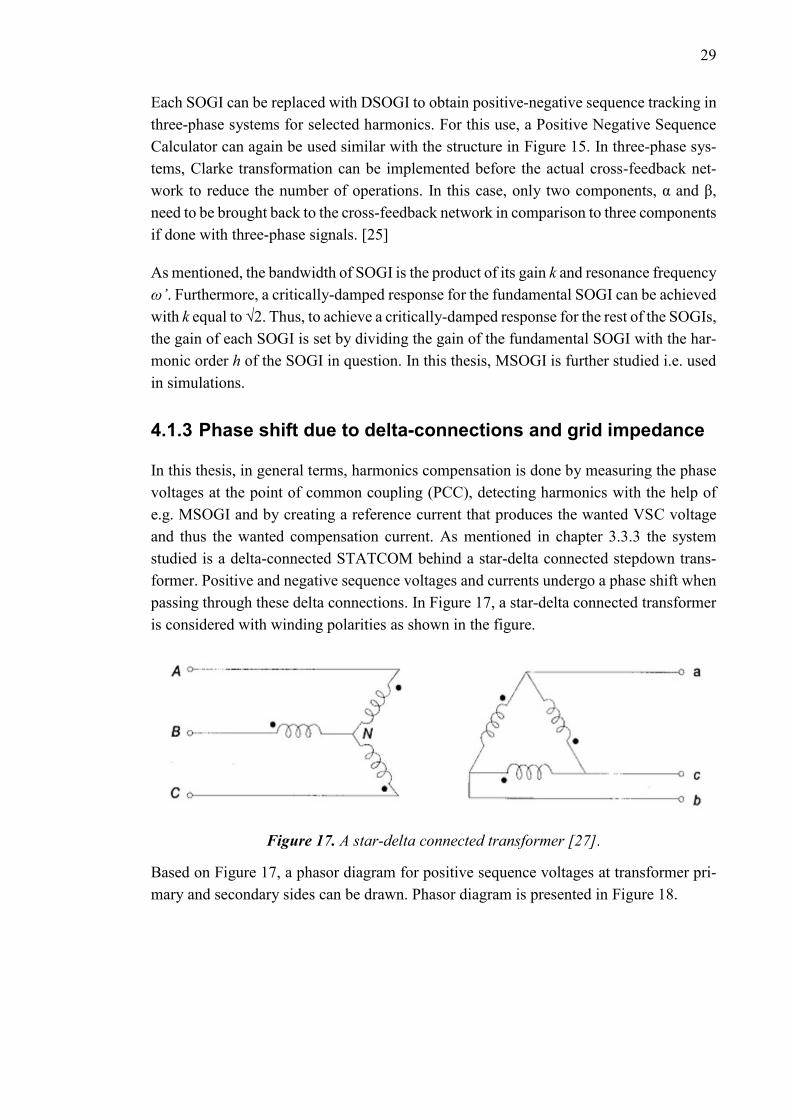
passing through these delta connections. In Figure 17, a star-delta connected transformer
is considered with winding polarities as shown in the figure.
Figure 17. A star-delta connected transformer [27].
Based on Figure 17, a phasor diagram for positive sequence voltages at transformer pri-
mary and secondary sides can be drawn. Phasor diagram is presented in Figure 18.
Page 38
30
Figure 18. Positive sequence voltages on Yd1 transformer [27].
The notation is done so that VAB1, VBC1, VCA1 are the line-to-line voltages and VAN1, VBN1,
VCN1 are the phase voltages on the primary star side. Respectively, Vab1, Vbc1 and Vca1
denote the corresponding line-to-line voltages on the secondary delta side. As can be seen,
the positive sequence line voltages on star side lead the corresponding delta side quanti-
ties by 30 degrees. The same phase shifts are also valid for currents. The transformer in
Figure 17 is thus Yd1 type of transformer.
If negative sequence voltages are considered, the phase shift reverse. A phasor diagram
is presented in Figure 19 to illustrate the phase shifts in case of negative sequence quan-
tities.
Figure 19. Negative sequence voltages on Yd1 transformer [27].
Page 39
31
As can be seen in Figure 19, for negative sequence voltages the phase shift is reverse
which means that the star side quantities lag delta side quantities by 30 degrees.
In this thesis, Yd11 type of transformer is used which means that for positive sequence
quantities delta side leads by 30 degrees and respectively for negative sequence quantities
star side leads by 30 degrees. [26] Moreover, due to delta-connected STATCOM branches
additional 30 degrees phase shifts occur when the produced compensation current passes
through the STATCOM delta-connection. The positive sequence quantities in STAT-
COM’s delta-connection lead by 30 degrees whereas the negative sequence quantities in
delta-connection lag by 30 degrees in respect to corresponding quantities outside the
delta-connection. In other words, positive and negative sequence quantities undergo alto-
gether 60 degrees phase shifts (to reverse directions) due to Yd11 type of transformer and
the delta-connected STATCOM branches.
In addition to delta-connections’ phase shifts, to be able to implement harmonics com-
pensation accurately, the grid impedance should also be known. The grid impedance
causes a phase shift between the injected harmonic compensation current and the resulting
voltage drop which thus needs to be taken into account similar with the phase shifts
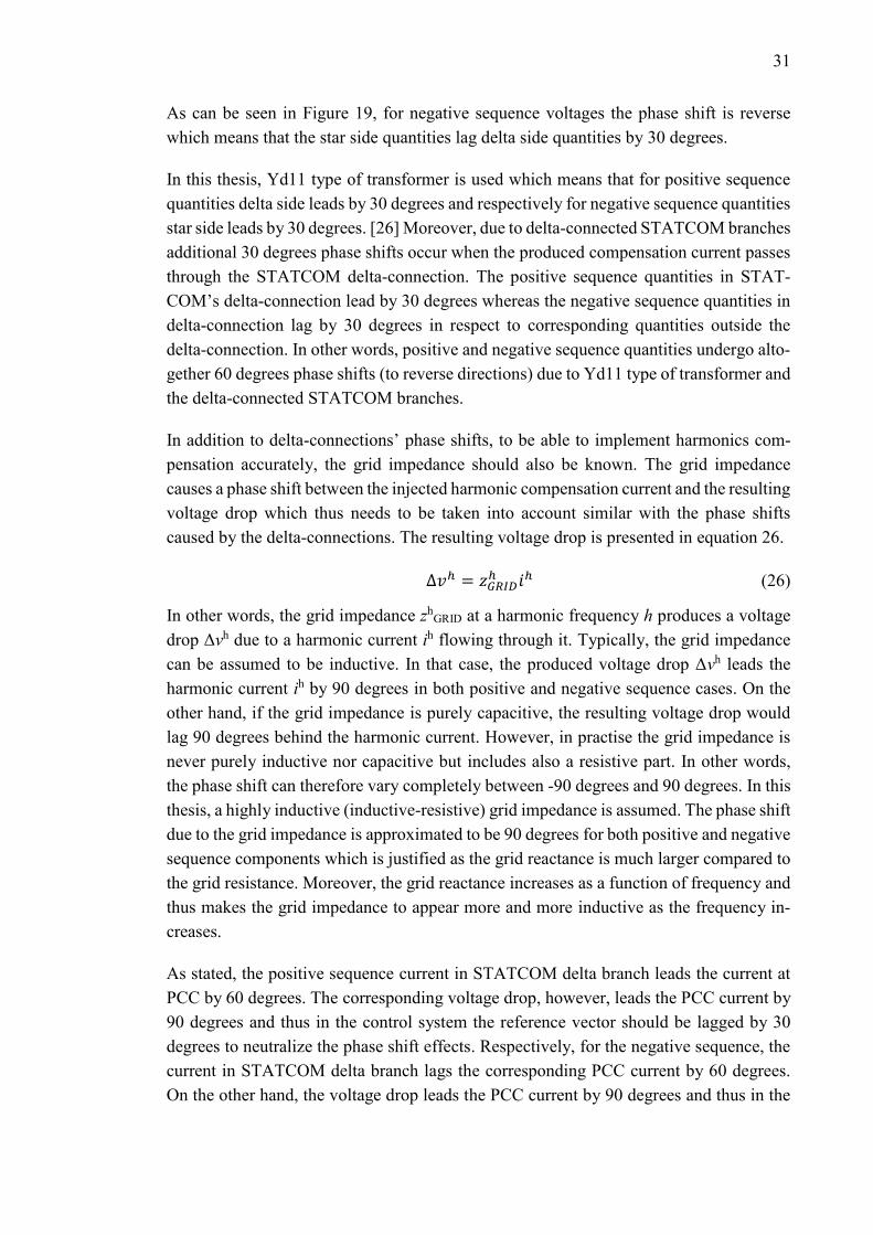
caused by the delta-connections. The resulting voltage drop is presented in equation 26.
∆𝑣ℎ = 𝑧𝐺𝑅𝐼𝐷ℎ 𝑖ℎ (26)
In other words, the grid impedance zhGRID at a harmonic frequency h produces a voltage
drop Δvh due to a harmonic current ih flowing through it. Typically, the grid impedance
can be assumed to be inductive. In that case, the produced voltage drop Δvh leads the
harmonic current ih by 90 degrees in both positive and negative sequence cases. On the
other hand, if the grid impedance is purely capacitive, the resulting voltage drop would
lag 90 degrees behind the harmonic current. However, in practise the grid impedance is
never purely inductive nor capacitive but includes also a resistive part. In other words,
the phase shift can therefore vary completely between -90 degrees and 90 degrees. In this
thesis, a highly inductive (inductive-resistive) grid impedance is assumed. The phase shift
due to the grid impedance is approximated to be 90 degrees for both positive and negative
sequence components which is justified as the grid reactance is much larger compared to
the grid resistance. Moreover, the grid reactance increases as a function of frequency and
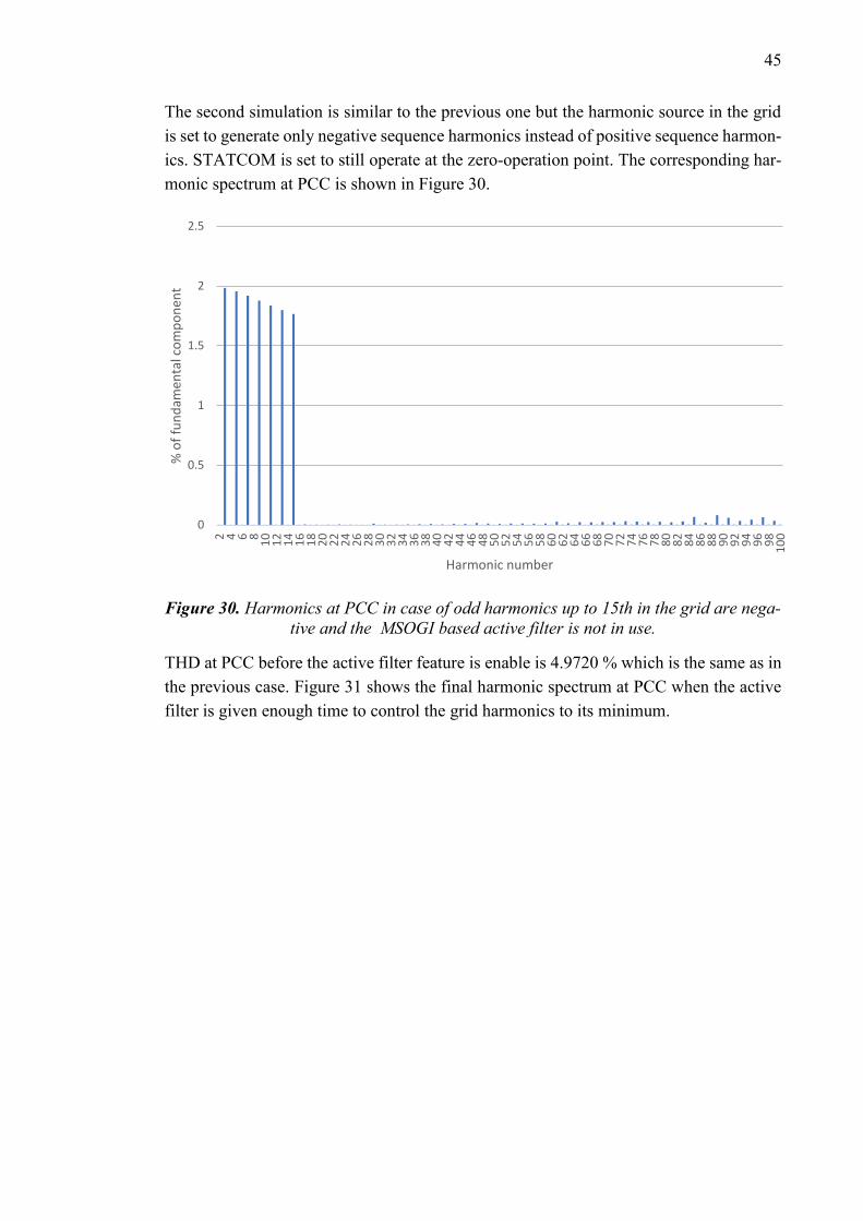
thus makes the grid impedance to appear more and more inductive as the frequency in-
creases.
As stated, the positive sequence current in STATCOM delta branch leads the current at
PCC by 60 degrees. The corresponding voltage drop, however, leads the PCC current by
90 degrees and thus in the control system the reference vector should be lagged by 30
degrees to neutralize the phase shift effects. Respectively, for the negative sequence, the
current in STATCOM delta branch lags the corresponding PCC current by 60 degrees.
On the other hand, the voltage drop leads the PCC current by 90 degrees and thus in the
Page 40
32
control system the reference vector should be lagged by 150 degrees to compensate the
phase shift effects.
Altogether, the phase shifts needed to compensate the effects of the star-delta connected
transformer, delta connected STATCOM as well as the grid impedance angle must be
implemented for positive and negative sequence components separately. In MSOGI this
can be done with a rotation matrix in the αβ-frame as αβ-components form a complex
plane. Individual rotation matrixes can be used for positive and negative sequence com-
ponents to enable separate positive-negative sequence phase control. The rotation matrix
is presented in the following equations 27 and 28.
𝑹(𝜃) = [𝑐𝑜𝑠 𝜃 −𝑠𝑖𝑛 𝜃𝑠𝑖𝑛 𝜃 𝑐𝑜𝑠 𝜃
] (27)
𝒗𝛼𝛽,𝑟𝑜𝑡𝑎𝑡𝑒𝑑 = 𝑹𝒗𝛼𝛽 (28)
The rotation matrix rotates the vector vαβ counter-clockwise by an angle θ introduced in
the rotation matrix resulting in a rotated voltage vector vαβ,rotated. If rotation to a clockwise
direction is wanted then a negative angle must be presented.
4.2 Synchronous reference frame
The detection and control of the fundamental voltage component can be done with the
help of synchronous reference frame (SRF). The main idea is to transform the rotating
three-phase components from the natural abc reference frame to DC values in the rotating
dq reference frame. This can be done by first using the Clarke transformation, as was
done also with SOGI, to transform the three-phase components to two inquadrature com-
ponents in the stationary reference frame and then applying the Park transformation. The
Park transformation makes the coordinate system to rotate to the same direction with the
same angular speed as αβ components. As a result, αβ components are transformed to a
voltage vector vdq i.e. d and q components, which are DC values, in the synchronous ref-
erence frame. [28] The Park transformation is presented in equations 29 and 30.
𝒗𝑑𝑞 = [𝑣𝑑
𝑣𝑞] = [𝑻𝑑𝑞]𝒗𝛼𝛽 (29)
[𝑻𝑑𝑞] = [𝑐𝑜𝑠 𝜃𝑠𝑦𝑛𝑐 𝑠𝑖𝑛 𝜃𝑠𝑦𝑛𝑐
−𝑠𝑖𝑛 𝜃𝑠𝑦𝑛𝑐 𝑐𝑜𝑠 𝜃𝑠𝑦𝑛𝑐] (30)
In equation 30, θsync is a so-called angular position which defines the rotation angle. As
can be noticed, the Park transformation is basically a rotation matrix which just rotates
the αβ components all the time to their reverse direction thus resulting in non-rotating d
and q components. The inverse Park transformation can be derived based on equation 30.
The angular position needed in the Park transformation is obtained conventionally by
using a Phase-Locked Loop (PLL) method. PLL gives the angle of the voltage component
Page 41
33
in reference to d component by controlling the voltage q component to zero. [28] The
structure of the PLL block is presented in Figure 20
Figure 20. Structure of the Phase-Locked Loop. Figure adapted from figure in [28].
As can be seen in Figure 20, a PI-controller is used to control the voltage q component to
zero. Moreover, a feedforward term ωff is used to speed up the frequency tracking and
finally the angular position θsync is obtained after integration of ωsync.
4.2.1 Decoupled Double Synchronous Reference Frame
For unbalanced grid conditions SRF-PLL can be upgraded to Decoupled Double Syn-
chronous Reference Frame PLL (DDSRF-PLL). It uses two different synchronous refer-
ence frames, one rotating to positive and the other rotating to negative direction. The
positive sequence of the fundamental component can thus be detected with the reference
frame rotating to positive direction while the negative sequence component can be de-
tected with the reference frame rotating to the inverse direction, respectively. [28]
Under unbalanced grid conditions the αβ components can be expressed as follows:
𝒗𝛼𝛽 = [𝑣𝛼
𝑣𝛽] = 𝑈+ [
𝑐𝑜𝑠(𝜔𝑡 + 𝜑+)
𝑠𝑖𝑛(𝜔𝑡 + 𝜑+)] + 𝑈− [
𝑐𝑜𝑠(−𝜔𝑡 + 𝜑−)
𝑠𝑖𝑛(−𝜔𝑡 + 𝜑−)], (31)
where ωt represents the angle of the fundamental frequency positive sequence component
i.e. θsync. U and φ in turn are the magnitude and the initial angle of the voltage vector.
Superscripts + and – denote the positive and negative sequence references, respectively.
[28] By using the above equation, the positive and negative sequence components can
also be expressed in the synchronous reference frame as follows:
𝒗𝑑𝑞+ = [
𝑣𝑑+
𝑣𝑞+] = [𝑻𝑑𝑞
+ ] [𝑣𝛼
𝑣𝛽] = [
𝑐𝑜𝑠(𝜔𝑡) 𝑠𝑖𝑛(𝜔𝑡)
−𝑠𝑖𝑛(𝜔𝑡) 𝑐𝑜𝑠(𝜔𝑡)] [
𝑣𝛼
𝑣𝛽] (32)
= 𝑈+ [cos(𝜑+)
sin(𝜑+)] + 𝑈− cos(𝜑−) [
cos(2𝜔𝑡)
−sin(2𝜔𝑡)] + 𝑈− sin(𝜑−) [
sin(2𝜔𝑡)
cos(2𝜔𝑡)]
Page 42
34
𝒗𝑑𝑞− = [
𝑣𝑑−
𝑣𝑞−] = [𝑻𝑑𝑞
− ] [𝑣𝛼
𝑣𝛽] = [
𝑐𝑜𝑠(𝜔𝑡) −𝑠𝑖𝑛(𝜔𝑡)
𝑠𝑖𝑛(𝜔𝑡) 𝑐𝑜𝑠(𝜔𝑡)] [
𝑣𝛼
𝑣𝛽] (33)
= 𝑈− [cos(𝜑−)
sin(𝜑−)] + 𝑈+ cos(𝜑+) [
cos(2𝜔𝑡)
sin(2𝜔𝑡)] + 𝑈+ sin(𝜑+) [
−sin(2𝜔𝑡)
cos(2𝜔𝑡)]
As can be noticed, under unbalanced grid conditions the positive and negative sequence
components in the synchronous reference frame consist of DC (Direct Current) and AC
(Alternating Current) components. The AC component occurring in the positive sequence
reference frame is due to a negative sequence component and the AC component taking
place in the negative sequence reference frame respectively is due to a positive sequence
component. In other words, under balanced grid conditions when the negative sequence
component can be assumed to be zero, the positive sequence component contains only
the DC component. A decoupling network is presented to cancel out these AC compo-
nents thus making it possible to represent the positive and negative sequence components
as pure DC components. The DC values can consequently be calculated as shown in equa-
tions 34 and 35.
𝑈+ [𝑐𝑜𝑠(𝜑+)
𝑠𝑖𝑛(𝜑+)] = [
𝑈𝑑+
𝑈𝑞+] = [
𝑣𝑑+
𝑣𝑞+] − 𝑈− 𝑐𝑜𝑠(𝜑−) [
𝑐𝑜𝑠(2𝜔𝑡)
−𝑠𝑖𝑛(2𝜔𝑡)] − 𝑈− 𝑠𝑖𝑛(𝜑−) [
𝑠𝑖𝑛(2𝜔𝑡)
𝑐𝑜𝑠(2𝜔𝑡)] (34)
𝑈− [𝑐𝑜𝑠(𝜑−)
𝑠𝑖𝑛(𝜑−)] = [
𝑈𝑑−
𝑈𝑞−] = [
𝑣𝑑−
𝑣𝑞−] − 𝑈+ 𝑐𝑜𝑠(𝜑+) [
𝑐𝑜𝑠(2𝜔𝑡)
𝑠𝑖𝑛(2𝜔𝑡)] − 𝑈+ 𝑠𝑖𝑛(𝜑+) [
−𝑠𝑖𝑛(2𝜔𝑡)
𝑐𝑜𝑠(2𝜔𝑡)] (35)
Ud and Uq represent the d and q component pure DC values after the AC components
have been cancelled out by the decoupling network. Superscripts + and – represent again
positive and negative sequence components, respectively. With the help of above pre-
sented decoupling network it is possible to present the desired sequence components as
pure DC values. [28]
The phase angle ωt needed for DDSRF is obtained with PLL similar with the way used
in SRF-PLL. The synchronization is done to positive sequence d component. In DDSRF-
PLL the PLL block controls the positive sequence q component to zero and thus makes it
also possible to represent the positive sequence voltage magnitude using only Ud+. [28]
The structure of the DDSRF-PLL block is presented in Figure 21.
Page 43
35
Figure 21. Structure of DDSRF-PLL. Figure adapted from figure in [28].
As can be seen in Figure 21, the positive sequence q component used for the synchroni-
zation in PLL is normalized to the positive sequence voltage component in order to make
the PLL gain remain constant independent of the network voltage magnitude. Moreover,
simple low-pass filters are used to extract the DC components for the outputs and for the
decoupling networks. [28] A transfer function for the simple low-pass filter is presented
in equation 36:
𝐿𝑃𝐹(𝑠) = 𝜔𝑓
𝑠+𝜔𝑓, (36)
where ωf is the cut-off frequency. The overbars, used in Figure 21, are to clarify that the
corresponding values are really DC values. After a transition period, also the values be-
fore low-pass filters are DC values if harmonics are ignored.
In ideal conditions when the grid doesn’t consist of any harmonics, the d and q compo-
nents are pure DC values after the decoupling network. However, if the grid contains
harmonics, these harmonics will also occur in the fundamental synchronous reference
frame d and q components. For example, the positive sequence component of the third
harmonic occurs as a 100 Hz component in Ud+ while the negative sequence component
of the third harmonic appears as a 200 Hz component, respectively. The same way, the
positive sequence of the second harmonic occurs as 50 Hz component and the negative
sequence of the second harmonic arises as 150 Hz component in Ud+. However, the low-
pass filters used after the DDSRF blocks filter out also these harmonics resulting in only
the DC values of the fundamental component to get through to output.
Page 44
36
4.2.2 Synchronous fundamental dq-frame
A common way to do harmonics compensation with the help of synchronous reference
frame is so called fundamental dq-frame method. As mentioned before, harmonics occur
as oscillations in the synchronous reference dq-frame. In other words, d and q components
consist of DC and AC components. In fundamental dq-frame method, the idea is to extract
the AC component as it is the harmonics part of the dq signal. [29, 30] Figure 22 illustrates
the idea of the fundamental dq-frame method.
Figure 22. Harmonics detection with fundamental dq-frame method.
As can be seen in Figure 22, at first the Park transformation is done to get vd and vq of the
fundamental frequency. These two components consist of DC and AC components when
the input signals contain harmonics. The DC parts are extracted with low-pass filters and
then subtracted from vd and vq resulting only the AC components to be taken further to
the inverse Park transformation. These components are presented in Figure 22 as vdh and
vqh. This way, after the inverse Park and the inverse Clarke transformations, the output
signals contain only harmonics which thus can be fed forward to cancel out the grid har-
monics. All in all, the fundamental dq-frame method gives the whole harmonic spectrum
as its output. If a selective harmonics detection and compensation is wanted then the fun-
damental dq-frame method is not the right choice. [30]
4.2.3 Synchronous harmonic dq-frame
In a harmonic dq-frame method, harmonics detection can be done selectively unlike in
the fundamental dq-frame method. The harmonic dq-frame uses individual dq-frames for
each harmonic component. In other words, each harmonic dq-frame rotates with an an-
gular speed equal to a specific harmonic. Otherwise the principle of this method is very
similar with the fundamental dq-frame method. For example, for the third harmonic a dq-
frame rotating at 150 Hz is implemented. Thus, vd and vq in this reference frame contain
the third harmonic as a DC component and other harmonics as well as the fundamental
frequency as an AC component. The detection of the specific harmonic component can
therefore be done by removing the AC component with a low-pass filter similar with the
fundamental dq-frame method. [29, 30] The principle of the harmonic dq-frame for a
detection of the 3rd, 5th and 7th harmonics is illustrated in Figure 23.
Page 45
37
Figure 23. Detection of the 3rd, 5th and 7th harmonics with the harmonic dq-frame
method.
As can be seen in Figure 23, each synchronous reference frame rotates according to a
specific harmonic frequency thus making the wanted harmonic to appear as a DC com-
ponent after the Park transformation. Low-pass filters are used to remove the AC compo-
nents as explained earlier. The phase angle needed for each Park transformation is taken
from the PLL based on the fundamental frequency dq-frame. This angle is scaled by a
coefficient which consequently determines the order of the harmonic to be detected. As a
result, after low-pass filters and the inverse Park and Clarke transformations, harmonic
components in the natural abc reference frame are provided as outputs. [29, 30] However,
as the conventional PLL is prone to inaccuracy when the grid contains a great number of
harmonics, a bandpass filter can be used to let only the fundamental frequency component
pass through to the fundamental SRF-PLL block. Thus, the accuracy of the synchroniza-
tion angle increases and the error especially for higher frequency dq-frames decreases.
This harmonic dq-frame method can be extended by adding new harmonic dq-frames for
all harmonics that need to be detected and compensated. Moreover, the harmonic dq-
frame method can be upgraded by using individual DDSRF blocks to enable positive-
negative sequence detections of different harmonics.
The low-pass filter has zero phase shift for DC components and thus the harmonic dq-
frame doesn’t have the issue with the phase shift because of the low-pass filter as the
harmonic component occurs as a DC component after the Park transformation. However,
as the fundamental frequency component is significantly larger compared to harmonic
components the output of the Park transformation occurs to have a substantial AC com-
ponent. As a result, the cut-off frequency of the low-pass filter needs to be set very low
to eliminate the impact of this AC component. This on the other hand leads to degraded
response time. To overcome this issue a cross-feedback network, a plain version of the
cross-feedback network used with MSOGI, is developed. Simply, a fundamental dq-
Page 46
38
frame can be used to detect the fundamental frequency component which then is con-
verted to the stationary reference frame (αβ components) and subtracted from the input
signal. Thus, the input signals of each harmonic Park transformation block won’t contain
the fundamental frequency component anymore. Respectively, the outputs of each Park
transformation block won’t contain a significant AC component and furthermore the cut-
off frequency of the low-pass filter can be set in a way to achieve an acceptable response
time.
As it was with MSOGI, the reference vectors in the control system need to be phase
shifted to neutralize the effects of the star-delta connected transformer, delta connected
STATCOM as well as the grid impedance angle. The phase shifting can be done with a
rotation matrix in the αβ-frame similar with the method used in SOGI. However, the
needed phase shift is possible to be implemented correspondingly in a harmonic dq-
frame. The d and q components can be converted from rectangular form to polar form as
presented in equations 37 and 38.
𝑀𝑎𝑔 = √𝑈𝑑2 + 𝑈𝑞
2 (37)
𝐴𝑛𝑔 = 𝑡𝑎𝑛−1 (𝑈𝑞
𝑈𝑑) (38)
The above equations provide magnitude and angle in the harmonic dq-frame and thus the
phase shift can easily be implemented in polar form by summing up the polar form angle
and the needed phase shift. Polar coordinates can then be converted back to rectangular
form i.e. back to d and q components. The presented method to implement the phase shift
in the dq-frame is easy to understand and thus practical. However, the most optimal so-
lution to implement the required phase shift is to do it by simply rotating the dq-frame
coordinate system. In other words, by adding the wanted phase shift to the synchroniza-
tion angle before the inverse Park transformation the reference vector can be rotated by
using only one sum operator.
The harmonic dq-frame method is widely used in active filter applications due to well-
covered literature of the dq-theory and the possibility to selectively control separate har-
monics [29]. Moreover, the control can be done by using DC values which makes the
whole control design simpler. In this thesis, the harmonic dq-frame method is further
studied i.e. used in simulations as it is capable of selective harmonics detection which is
wanted.
Page 47
39
5. SIMULATIONS
In this chapter, simulations are done for the MSOGI based method and for the synchro-
nous harmonic dq-frame method (later SRF based method). The studied methods are im-
plemented into an existing STATCOM simulation model in PSCAD environment where
the simulations are correspondingly carried out. The simulation model consists of an ideal
grid voltage source, a separate series connected harmonic voltage source, grid impedance,
a wye-delta connected transformer and the actual STATCOM system. In a simplified sin-
gle line diagram, presented in Figure 24, the ideal grid voltage source and the series con-
nected harmonic voltage source are presented as a single grid voltage source.
Figure 24. Simplified single line diagram of the circuit used for simulations.
In the simulation model, STATCOM is modelled as a voltage source converter whose
three-phase voltages are produced by a control system. The actual simulation model in-
cludes several parts not shown in the single line diagram. However, those are not relevant
for the understanding of this work. In general terms, in this thesis, harmonics compensa-
tion is done by measuring the phase voltages at the point of common coupling (PCC),
detecting harmonics with the help of studied methods and by creating a reference current
that together with the reactive power compensation reference current produces the wanted
VSC voltage and thus the wanted actual compensation current. The harmonic compensa-
tion reference current in the control system with the MSOGI based method is created
from the detected voltage harmonics by a PR-controller already existing in the used sim-
ulation model. Respectively, with the SRF based method, the corresponding reference
Page 48
40
current is created from the detected voltage harmonics by a simple integrator (I-control-
ler). Tunings of the controllers are not further considered in this thesis as only simulations
in steady-state cases are done. Also, the control of the entire STATCOM system is not
considered in more detail as the basic understanding of the operation is enough regarding
this thesis.
In this thesis, odd harmonics up to 15th harmonic order are to be compensated. Thus, the
implemented MSOGI based method consists of eight DSOGI blocks, seven blocks for
harmonics and one for the fundamental, with a corresponding cross-feedback network
and the implemented SRF based method of seven harmonic dq-frames and one funda-
mental dq-frame, respectively.
5.1 Simulation settings
In the first simulations, the harmonic voltage source is set to generate odd harmonics up
to 15th harmonic according to Table 3.
Table 3. Grid harmonics for the first simulations.
Harmonic order
3 5 7 9 11 13 15
Harmonic voltage %
of the funda-mental
2 2 2 2 2 2 2
Other harmonics are set to zero. This is to get reference how each method performs when
the grid contains only harmonics the active filter is set to compensate. Standard IEC
61000-3-6 presents indicative planning levels for harmonic voltages up to 50th harmonic.
The planning levels were presented in Table 2 earlier. These planning levels are used in
later simulations to create appropriate number of harmonics in the grid to demonstrate the
performance in real life situation. The voltage THD calculated from the individual har-
monic limits is 5.33 %. However, standard IEC 61000-3-6 also presents indicative level
of 3 % for total harmonic distortion which thus will not be met if the grid harmonics are
set according to individual harmonic limits. Harmonics are thus scaled by a factor of 0.55
to meet the presented voltage THD. The standard defines only harmonic limits up to 50th
harmonic but not above. However, the grid is wanted to contain also higher order har-
monics and thus voltage magnitude of 0.1 % of the fundamental component is added for
harmonic orders between 51 and 100. The resulting voltage THD is 3.015 %. The angles
of the harmonics in respect to the fundamental voltage angle are set to zero degrees. The
used harmonic spectrum is presented in Figure 25.
Page 49
41
Figure 25. Voltage harmonic spectrum used for background distortion.
The grid harmonics are generated by the harmonic voltage source in the grid. Harmonic
spectrums at PCC will be different as the simulation model has grid impedance between
the harmonic voltage source and PCC.
Simulation results are realized by extracting harmonics from measured waveforms with
a Fast Fourier Transform block in PSCAD and further by exporting data to Excel for
calculations and graph drawing. Relevant system parameters for the simulations are pre-
sented in Appendix A.
5.2 Performance of the MSOGI method
In this subchapter, the performance of the studied MSOGI based active filter method is
simulated in steady-state cases. Simulations are done to demonstrate the performance of
the MSOGI based method in case of positive and negative sequence harmonics, in STAT-
COM’s different operation points and under highly distorted circumstances.
5.2.1 Positive and negative sequence filtering with MSOGI
The first two simulations are done to perceive how well MSOGI performs when the grid
contains mostly the harmonics MSOGI is set to compensate. STATCOM’s reactive power
compensation is at first set to the zero-operation point to narrow down its possible effects
on the active filtering. For the first simulation the harmonic source in the grid is set to
generate only positive sequence odd harmonics up 15th harmonic according to Table 3.
The corresponding harmonic spectrum at PCC can be seen in Figure 26.
0
0.2
0.4
0.6
0.8
1
1.2
2 4 6 81
01
21
41
61
82
02
22
42
62
83
03
23
43
63
84
04
24
44
64
85
05
25
45
65
86
06
26
46
66
87
07
27
47
67
88
08
28
48
68
89
09
29
49
69
81
00
% o
f fu
nd
amen
tal c
om
po
nen
t
Harmonic number
Page 50
42
Figure 26. Harmonics at PCC in case of odd harmonics up to 15th in the grid are posi-
tive and the MSOGI based active filter is not in use.
Harmonic spectrum is shown all the way up to 100th harmonic to ensure the active har-
monic filter will not only compensate the harmonics it is set to compensate but also that
it will not significantly increase other harmonics while compensating. Harmonics at PCC
are lower compared to the values set for the harmonic voltage source in the grid. This is
naturally due to inductive grid impedance between the voltage source and PCC that line-
arly increases as a function of increasing frequency causing different amount of voltage
drop to occur for different harmonics. Also, even though the harmonic source is set to
generate only odd harmonics up to 15th harmonic, other harmonics can still be noticed to
occur at PCC. This is due to STATCOM’s normal operation when creating the funda-
mental voltage component even at its zero-operation point. Voltage THD at PCC before
harmonics control is enabled is 4.9720 %. Figure 27 shows the final harmonic spectrum
at PCC when the active filter is given enough time to control the grid harmonics to the
smallest possible.
0
0.5
1
1.5
2
2.5
2 4 6 81
01
21
41
61
82
02
22
42
62
83
03
23
43
63
84
04
24
44
64
85
05
25
45
65
86
06
26
46
66
87
07
27
47
67
88
08
28
48
68
89
09
29
49
69
81
00
% o
f fu
nd
amen
tal c
om
po
nen
t
Harmonic number
Page 51
43
Figure 27. Harmonics at PCC in case of odd harmonics up to 15th in the grid are posi-
tive and the MSOGI based active filter is in use.
As can be seen in Figure 27, the controlled harmonics settle down very close to zero.
Moreover, even if some variety in other harmonics may be seen, no significant increase
in individual harmonic components is still noticed. The final voltage THD at PCC is
0.1518 % which implies the voltage waveform to be almost an ideal sinewave. Figure 28,
furthermore, presents the PCC voltage waveforms in time domain before the active har-
monic filter control is enabled and after the grid harmonics have been compensated to the
smallest possible.
0
0.01
0.02
0.03
0.04
0.05
0.06
0.07
0.08
0.09
0.1
2 4 6 81
01
21
41
61
82
02
22
42
62
83
03
23
43
63
84
04
24
44
64
85
05
25
45
65
86
06
26
46
66
87
07
27
47
67
88
08
28
48
68
89
09
29
49
69
81
00
% o
f fu
nd
amen
tal c
om
po
nen
t
Harmonic number
Page 52
44
Figure 28. Voltage waveform at PCC before and after active filtering.
As can be seen in Figure 28, the final voltage waveform is noticeably less distorted com-
pared to the initial voltage waveform after harmonics have been compensated. To further
illustrate the real-time active filtering, Figure 29 presents the compensation of the 7th har-
monic as a function of time.
Figure 29. Filtering of the 7th harmonic.
As can be seen in Figure 29, the 7th harmonic decreases smoothly after active filter control
is enabled (t = 0.25 s) and in the end, settles down to zero as perceived also before.
Page 53
45
The second simulation is similar to the previous one but the harmonic source in the grid
is set to generate only negative sequence harmonics instead of positive sequence harmon-
ics. STATCOM is set to still operate at the zero-operation point. The corresponding har-
monic spectrum at PCC is shown in Figure 30.
Figure 30. Harmonics at PCC in case of odd harmonics up to 15th in the grid are nega-
tive and the MSOGI based active filter is not in use.
THD at PCC before the active filter feature is enable is 4.9720 % which is the same as in
the previous case. Figure 31 shows the final harmonic spectrum at PCC when the active
filter is given enough time to control the grid harmonics to its minimum.
0
0.5
1
1.5
2
2.52 4 6 8
10
12
14
16
18
20
22
24
26
28
30
32
34
36
38
40
42
44
46
48
50
52
54
56
58
60
62
64
66
68
70
72
74
76
78
80
82
84
86
88
90
92
94
96
98
10
0
% o
f fu
nd
amen
tal c
om
po
nen
t
Harmonic number
Page 54
46
Figure 31. Harmonics at PCC in case of odd harmonics up to 15th in the grid are nega-
tive and the MSOGI based active filter is in use.
As can be seen in Figure 31, the controlled harmonics settle down again very close to
zero and similar to the first simulation no significant increase in other harmonics is no-
ticed. The final THD at PCC is 0.1335 % that is close to the final THD in the positive
sequence case. As a result, MSOGI can be considered to perform the same way for both
positive and negative sequence harmonics. The next simulations are done by using only
positive sequence harmonics to decrease the number of simulations.
5.2.2 MSOGI under distorted circumstances
To test MSOGI’s performance under highly distorted circumstances the harmonic source
in the grid is set to generate harmonics according to standard’s IEC 61000-3-6 planning
levels. STATCOM is at first set to operate at its zero-operation point similar to the previ-
ous simulations and later set to its maximum capacitive and maximum inductive operation
points. The harmonic source in the grid is set to generate only positive sequence harmon-
ics. The corresponding harmonic spectrum at PCC before the active filter control is ena-
bled is presented in Figure 32.
0
0.01
0.02
0.03
0.04
0.05
0.06
0.07
0.08
0.09
0.1
2 4 6 81
01
21
41
61
82
02
22
42
62
83
03
23
43
63
84
04
24
44
64
85
05
25
45
65
86
06
26
46
66
87
07
27
47
67
88
08
28
48
68
89
09
29
49
69
81
00
% o
f fu
nd
amen
tal c
om
po
nen
t
Harmonic number
Page 55
47
Figure 32. Harmonics at PCC in case of positive sequence harmonics set up to 100th
according to IEC 61000-3-6 and the MSOGI based active filter is not in use.
THD at PCC is 2.7772 %. Figure 33 shows the final harmonic spectrum at PCC after the
active filter control is enabled and it is given enough time to control the grid harmonics
to the smallest possible.
Figure 33. Harmonics at PCC in case of positive sequence harmonics set up to 100th
according to IEC 61000-3-6 and the MSOGI based active filter is in use.
As can be seen in Figure 33, the controlled odd harmonics settle down very close to zero
even when the grid contains a great number of other harmonics. Some increase can be
0
0.2
0.4
0.6
0.8
1
1.2
2 4 6 81
01
21
41
61
82
02
22
42
62
83
03
23
43
63
84
04
24
44
64
85
05
25
45
65
86
06
26
46
66
87
07
27
47
67
88
08
28
48
68
89
09
29
49
69
81
00
% o
f fu
nd
amen
tal c
om
po
nen
t
Harmonic number
0
0.2
0.4
0.6
0.8
1
1.2
2 4 6 81
01
21
41
61
82
02
22
42
62
83
03
23
43
63
84
04
24
44
64
85
05
25
45
65
86
06
26
46
66
87
07
27
47
67
88
08
28
48
68
89
09
29
49
69
81
00
% o
f fu
nd
amen
tal c
om
po
nen
t
Harmonic number
Page 56
48
seen in other harmonics with the maximum increase of 0.16 % at the 23rd harmonic but
overall no significant increase is still noticed. Final THD at PCC is 1.7765 % which is
considerably smaller than the initial THD at PCC (2.7772 %).
As the active harmonic filter feature is meant to operate simultaneously with the reactive
power compensation, simulations at the maximum capacitive and at the maximum induc-
tive operation points should be performed. Simulation settings are otherwise similar with
the previous simulation but now STATCOM’s reactive power compensation is set to its
maximum capacitive operation point. The corresponding harmonic spectrum at PCC can
be seen in Figure 34.
Figure 34. Harmonics at PCC in case of STATCOM operating at its maximum capaci-
tive operation point and the MSOGI based active filter is not in use.
THD at PCC before the active filter control is enabled is 2.6342 %. As can be seen in
Figure 34, harmonics tend to be smaller in terms of percentage of the fundamental com-
ponent compared to the previous case when STATCOM’s reactive power compensation
was set to the zero-operation point. This is due to the capacitive power compensation
which increases the fundamental voltage at PCC resulting in harmonic components to be
smaller in terms of percentage. The relation between the grid voltage and the PCC voltage
can be presented according to Kirchhoff’s voltage law as follows:
𝑉𝐺𝑅𝐼𝐷 = 𝑉𝑃𝐶𝐶 + 𝑍𝐺𝑅𝐼𝐷𝐼𝑄, (39)
where VGRID is the grid voltage, VPCC is the voltage at PCC, ZGRID is the grid impedance
and IQ is the reactive current produced by STATCOM. In Figure 35 phasor diagrams for
capacitive and inductive operations points are illustrated based on equation 39. The grid
impedance is assumed to be purely inductive to simplify drawings.
0
0.2
0.4
0.6
0.8
1
1.2
2 4 6 81
01
21
41
61
82
02
22
42
62
83
03
23
43
63
84
04
24
44
64
85
05
25
45
65
86
06
26
46
66
87
07
27
47
67
88
08
28
48
68
89
09
29
49
69
81
00
% o
f fu
nd
amen
tal c
om
po
nen
t
Harmonic number
Page 57
49
Figure 35. The impact of A) capacitive and B) inductive current to PCC voltage.
As can be seen in Figure 35A), when STATCOM generates capacitive current, it leads to
an increase in the fundamental VPCC magnitude. However, harmonic voltages Vh remain
the same at PCC which thus results in them to appear smaller in terms of percentage
compared to the results when STATCOM was operated at its zero-operation point. Re-
spectively, when STATCOM is operated at the inductive side, the fundamental VPCC mag-
nitude decreases as can also be noticed in Figure 35B). Naturally, as absolute values of
harmonic voltages remain the same, the harmonic voltages appear to be greater in terms
of percentage compared to STATCOM’s zero-operation and capacitive operation results.
Figure 36 shows the final harmonic spectrum after enough time is given for the active
filter control to compensate the grid harmonics to its minimum.
Figure 36. Harmonics at PCC in case of STATCOM operating at its maximum capaci-
tive operation point and the MSOGI based active filter is in use.
As can be seen in Figure 36, the controlled odd harmonics settle down very close to zero
also when operating in the maximum capacitive operation point. Final THD at PCC is
0
0.2
0.4
0.6
0.8
1
1.2
2 4 6 81
01
21
41
61
82
02
22
42
62
83
03
23
43
63
84
04
24
44
64
85
05
25
45
65
86
06
26
46
66
87
07
27
47
67
88
08
28
48
68
89
09
29
49
69
81
00
% o
f fu
nd
amen
tal c
om
po
nen
t
Harmonic number
Page 58
50
1.6773 % that is slightly smaller than earlier when STATCOM’s reactive power compen-
sation was set to zero-operation point. This, however, can be explained by the nature of
capacitive power compensation that increases the fundamental voltage at PCC as men-
tioned before. Absolute values of harmonic components are still very close to the same.
Finally, the MSOGI based active filter feature is simulated in STATCOM’s maximum
inductive operation point. The corresponding harmonic spectrum at PCC is shown in Fig-
ure 37.
Figure 37. Harmonics at PCC in case of STATCOM operating at its maximum induc-
tive operation point and the MSOGI based active filter is not in use.
THD at PCC before the active filter control is enabled is 2.9376 %. As predicted, har-
monics are mainly larger in terms of percentage than in previous cases due to inductive
power compensation. Figure 38 shows the final harmonic spectrum after enough time is
given for the active filter control to compensate the grid harmonics to the smallest possi-
ble.
0
0.2
0.4
0.6
0.8
1
1.2
2 4 6 81
01
21
41
61
82
02
22
42
62
83
03
23
43
63
84
04
24
44
64
85
05
25
45
65
86
06
26
46
66
87
07
27
47
67
88
08
28
48
68
89
09
29
49
69
81
00
% o
f fu
nd
amen
tal c
om
po
nen
t
Harmonic number
Page 59
51
Figure 38. Harmonics at PCC in case of STATCOM operating at its maximum induc-
tive operation point and the MSOGI based active filter is in use.
As can be seen in Figure 38, the controlled odd harmonics settle down very close to zero
as well when operating at the maximum inductive operation point. Final THD at PCC is
1.8679 % that is greater than earlier when STATCOM was set to operate at its maximum
capacitive operation point (1.6773 %). The greater final THD can be explained by the
nature of inductive power compensation that decreases the fundamental voltage compo-
nent at PCC. Absolute values of harmonic components are thus very close to those when
STATCOM was operated at its capacitive and zero-operation points. The decrease from
the initial THD at PCC can also be considered significant.
The MSOGI based active filter method can be considered to operate properly in all three
operation points simulated (zero-operation, maximum capacitive and maximum induc-
tive) even when the grid contains a great number of other harmonics.
5.3 Performance of the SRF based method
In this subchapter, the performance of the studied harmonic dq-frame based (SRF based)
active filter method is simulated in steady-state cases. Simulations are done to demon-
strate the performance of the SRF based method in case of positive and negative sequence
harmonics, in STATCOM’s different operation points and under highly distorted circum-
stances. The simulations are analogous with the simulations done with MSOGI.
0
0.2
0.4
0.6
0.8
1
1.2
2 4 6 81
01
21
41
61
82
02
22
42
62
83
03
23
43
63
84
04
24
44
64
85
05
25
45
65
86
06
26
46
66
87
07
27
47
67
88
08
28
48
68
89
09
29
49
69
81
00
% o
f fu
nd
amen
tal c
om
po
nen
t
Harmonic number
Page 60
52
5.3.1 Positive and negative sequence filtering with SRF
The first simulations for the SRF based method are done to observe how well harmonics
can be compensated when the grid contains only the harmonics SRF based active filter is
set to compensate. The harmonic compensation shouldn’t either generate significantly
any other harmonics to the grid. At first, the harmonic voltage source in the grid is set to
generate only positive sequence odd harmonics up to 15th harmonic to the grid according
to Table 3. STATCOM is set to operate at its zero-operation point. The harmonic spec-
trum at PCC before harmonic compensation is enabled is similar with the spectrum pre-
sented earlier in Figure 26. The harmonic spectrum after the SRF based active filter con-
trol is given enough time to control the harmonics to its smallest possible is shown in
Figure 39.
Figure 39. Harmonics at PCC in case of odd harmonics up to 15th in the grid are posi-
tive and the SRF based active filter is in use.
As can be seen in Figure 39, the controlled odd harmonics settle down very close to zero.
The final values of the controlled harmonics are almost equal with the results got with
MSOGI. Also, the absolute values of other harmonics are very close to those with MSOGI
i.e. no significant increase in uncontrolled harmonics can be noticed. The final THD at
PCC settles down to 0.1508 % which is thus almost identical with the final THD got with
MSOGI (0.1518 %).
The second simulation is done by setting the harmonic source in the grid to generate only
negative sequence odd harmonics up to 15th harmonic instead of positive sequence har-
monics. Otherwise the simulation is similar with the previous one. The harmonic spec-
trum at PCC before the active filter control is enabled is similar with the spectrum pre-
sented earlier in Figure 30. The final harmonic spectrum at PCC after the SRF based
0
0.01
0.02
0.03
0.04
0.05
0.06
0.07
0.08
0.09
0.1
2 4 6 81
01
21
41
61
82
02
22
42
62
83
03
23
43
63
84
04
24
44
64
85
05
25
45
65
86
06
26
46
66
87
07
27
47
67
88
08
28
48
68
89
09
29
49
69
81
00
% o
f fu
nd
amen
tal c
om
po
nen
t
Harmonic number
Page 61
53
active filter control is given enough time to control the harmonics to the smallest possible
is presented in Figure 40.
Figure 40. Harmonics at PCC in case of odd harmonics up to 15th in the grid are nega-
tive and the SRF based active filter is in use.
The controlled harmonics settle down again very close to zero as can be seen in Figure
40. The final values of controlled harmonics are almost identical with the results got with
MSOGI. Similar to the previous simulation, no significant increase either in other har-
monics can be noticed. The final THD at PCC settles down to 0.1331 % which is again
practically the same as the final THD got with MSOGI (0.1335 %). The SRF based active
filter feature can be stated to perform almost similarly for both positive and negative se-
quence harmonics. As a consequence, the next simulations are done by using only posi-
tive sequence harmonics to reduce the number of simulations.
5.3.2 SRF under distorted circumstances
To test SRF based active filter feature under distorted circumstances the harmonic source
in the grid is set to generate harmonics according to standard’s IEC 61000-3-6 planning
levels. STATCOM is at first set to operate at its zero-operation point similar to previous
simulations and then set to its maximum capacitive and maximum inductive operation
points. The harmonic source in the grid is set to generate only positive sequence harmon-
ics. The harmonic spectrum at PCC before the active filter control is enabled is similar
with the spectrum presented earlier in Figure 32. The final THD at PCC after the active
filter control is given enough time to control the grid harmonics to the smallest possible
is presented in Figure 41.
0
0.01
0.02
0.03
0.04
0.05
0.06
0.07
0.08
0.09
0.1
2 4 6 81
01
21
41
61
82
02
22
42
62
83
03
23
43
63
84
04
24
44
64
85
05
25
45
65
86
06
26
46
66
87
07
27
47
67
88
08
28
48
68
89
09
29
49
69
81
00
% o
f fu
nd
amen
tal c
om
po
nen
t
Harmonic number
Page 62
54
Figure 41. Harmonics at PCC in case of positive sequence harmonics set up to 100th
according to IEC 61000-3-6 and the SRF based active filter is in use.
As can be seen in Figure 41, all the controlled harmonics decrease to zero even when the
grid contains a great number of other harmonics. The final values of the controlled har-
monics are very close to the corresponding final values got with MSOGI and thus the
SRF based method can be considered capable of compensating selected harmonics prac-
tically completely. The uncontrolled harmonics remain very close to the initial situation
with only some variety. The final THD at PCC settles down to 1.6895 % which is roughly
0.1 % smaller than the corresponding final THD got with MSOGI (1.7765 %). The final
THD is also considerably smaller than the initial THD 2.7772 %.
The SRF based active filter feature is tested also in the maximum capacitive and maxi-
mum inductive operations points. Otherwise, the simulation settings are the same but now
STATCOM is set to operate at its maximum capacitive operation point. The correspond-
ing harmonic spectrum at PCC before the active filter feature is enabled is similar with
the spectrum presented earlier in Figure 34. The final harmonic spectrum at PCC before
the active filter control is enabled is shown in Figure 42.
0
0.2
0.4
0.6
0.8
1
1.2
2 4 6 81
01
21
41
61
82
02
22
42
62
83
03
23
43
63
84
04
24
44
64
85
05
25
45
65
86
06
26
46
66
87
07
27
47
67
88
08
28
48
68
89
09
29
49
69
81
00
% o
f fu
nd
amen
tal c
om
po
nen
t
Harmonic number
Page 63
55
Figure 42. Harmonics at PCC in case of STATCOM operating at its maximum capaci-
tive operation point and the SRF based active filter is in use.
As can be seen in Figure 42, the controlled harmonics decrease to zero. Similar to the
previous simulation, the harmonic compensation performance remains high even when
the grid contains a great number of other harmonics. Moreover, no significant increase in
other harmonics can be noticed. Due to the operation at STATCOM’s maximum capaci-
tive operation point, the harmonics are smaller in terms of percentage compared to the
values got when STATCOM was operated at its zero-operation point. The final THD at
PCC settles down to 1.5940 % which is again slightly smaller than the final THD got with
MSOGI (1.6773 %) and thus also considerably smaller than the initial THD at PCC
(2.6342 %).
Finally, the SRF based active filter feature is tested when STATCOM is set to operate at
its maximum inductive operation point. The corresponding harmonic spectrum at PCC
before the active filter control is enabled is similar with the harmonic spectrum presented
earlier in Figure 37. The final harmonic spectrum at PCC after the active filter control is
given enough time to control the grid harmonics to the smallest possible is shown in Fig-
ure 43.
0
0.2
0.4
0.6
0.8
1
1.2
2 4 6 81
01
21
41
61
82
02
22
42
62
83
03
23
43
63
84
04
24
44
64
85
05
25
45
65
86
06
26
46
66
87
07
27
47
67
88
08
28
48
68
89
09
29
49
69
81
00
% o
f fu
nd
amen
tal c
om
po
nen
t
Harmonic number
Page 64
56
Figure 43. Harmonics at PCC in case of STATCOM operating at its maximum induc-
tive operation point and the SRF based active filter is in use.
The controlled harmonics decrease very close to zero also when STATCOM is operated
at its maximum inductive operation point as can be noticed in Figure 43. The impact to
uncontrolled harmonics is almost negligible but due to STATCOM’s operation at its max-
imum inductive operation point the harmonics are greater in terms of percentage of the
fundamental component compared to operations in the capacitive and zero-operation
points. The final THD at PCC settles down to 1.7789 % which is smaller than MSOGI’s
corresponding THD (1.8679 %) and also considerably smaller than the initial THD at
PCC (2.9376 %)
As a result, the SRF based active filter feature seems to perform similarly in all three,
zero, capacitive and inductive, operation points. The controlled harmonics decrease prac-
tically to zero in every case simulated and the difference in performances between the
SRF based method and the MSOGI based method especially in terms of final harmonic
component values can be considered negligible.
5.4 Capacitive grid impedance
In the simulations done in 5.2 and in 5.3 the grid impedance was assumed to be highly
inductive. Based on this assumption, corresponding phase shifts were implemented for
the reference vector in the control system. As a consequence, if the grid impedance occurs
to be capacitive at a certain harmonic frequency, the phase shifts done in the control sys-
tem wouldn’t be correct anymore and thus the active filter feature would start to amplify
that particular harmonic component instead of mitigating it. If the grid impedance is
0
0.2
0.4
0.6
0.8
1
1.2
2 4 6 81
01
21
41
61
82
02
22
42
62
83
03
23
43
63
84
04
24
44
64
85
05
25
45
65
86
06
26
46
66
87
07
27
47
67
88
08
28
48
68
89
09
29
49
69
81
00
% o
f fu
nd
amen
tal c
om
po
nen
t
Harmonic number
Page 65
57
known, the active filter control can be tuned in a way to achieve an optimal performance
even if the grid occurs to be capacitive.
The next simulation is done in order to demonstrate that harmonics can be compensated
also if the grid impedance occurs to be capacitive. The active filtering is done with the
studied MSOGI based method. In the simulation, a highly capacitive grid impedance is
assumed and thus the reference vector phase shift is changed in the control system to
obtain harmonics compensation correspondingly in the capacitive grid. With capacitive
grid, the grid impedance decreases as a function of increasing frequency. If the capacitive
grid impedance at the fundamental frequency is set equal with the grid impedance in case
of inductive grid, grid impedances at harmonic frequencies would differ a lot. Moreover,
the VSC current would need to be enormous to achieve great enough voltage change in
in the grid to cancel out the grid harmonics. Thus, the grid impedance is set in a way that
it is the same order of magnitude at the 3rd and 5th harmonic as it was in the case of
inductive grid. Consequently, the harmonic voltage source in the grid is set to only gen-
erate positive sequence components of 3rd and 5th harmonic according to Table 3. More-
over, STATCOM is set to operate at its zero-operation point. The corresponding harmonic
spectrum at PCC before the active filter control is enabled is presented in Figure 44.
Figure 44. Harmonic spectrum at PCC when the grid is highly capacitive and the
MSOGI based active filter is not in use.
THD at PCC before harmonic control is enabled is 2.8043 %. The fifth harmonic compo-
nent is slightly greater than the third harmonic due to the capacitive grid impedance. The
harmonic spectrum after the active filter has controlled the grid harmonics to the smallest
possible is presented in Figure 45.
0
0.2
0.4
0.6
0.8
1
1.2
2 4 6 81
01
21
41
61
82
02
22
42
62
83
03
23
43
63
84
04
24
44
64
85
05
25
45
65
86
06
26
46
66
87
07
27
47
67
88
08
28
48
68
89
09
29
49
69
81
00
% o
f fu
nd
amen
tal c
om
po
nen
t
Harmonic number
Page 66
58
Figure 45. Harmonic spectrum at PCC when the grid is highly capacitive and the
MSOGI based active filter is in use.
As can be seen in Figure 45, both harmonics, 3rd and 5th, settle down to zero. Even if some
variety in other harmonics may be seen, no significant increase in individual harmonic
components is still noticed. THD at PCC settles down very close to zero with the final
value of 0.0493 %.
As a result, it can be stated that the active harmonic filter works also in case of capacitive
grid. However, the grid impedance needs to be known or alternatively the control needs
to be designed in order to figure out if the grid occurs to be capacitive at certain harmonic
frequencies and further the corresponding phase shifts need to be implemented. If the grid
is assumed to be highly inductive and no additional control is designed to recognize ca-
pacitive grid impedance, the active filter may start to amplify harmonics instead of com-
pensating them.
0
0.01
0.02
0.03
0.04
0.05
0.06
0.07
0.08
0.09
0.1
2 4 6 81
01
21
41
61
82
02
22
42
62
83
03
23
43
63
84
04
24
44
64
85
05
25
45
65
86
06
26
46
66
87
07
27
47
67
88
08
28
48
68
89
09
29
49
69
81
00
% o
f fu
nd
amen
tal c
om
po
nen
t
Harmonic number
Page 67
59
6. ANALYSIS AND COMPARISON OF THE RE-
SULTS
Simulation results show that both of the studied methods, the MSOGI based method and
the SRF based method, are capable of compensating both positive and negative sequence
harmonics completely when the grid contains only harmonics STATCOM is set to com-
pensate. Both methods are also capable of compensating harmonics in STATCOM’s all
three operation points even when the grid contains a great number of other harmonics.
The difference in performances between the studied two methods in terms of final con-
trolled harmonic component values is negligible and thus both methods can be considered
to be able to compensate harmonics practically completely in steady-state. In terms of
final THD values, the SRF based method shows slightly better performance over the
MSOGI based method. If an ideal final THD was calculated from the initial situation so
that all controlled harmonics would completely decrease to zero and other harmonics
wouldn’t be affected, the final THD would be for example in case of zero-operation
1.6842 %. The corresponding final THD got with the SRF based method reaches almost
the ideal case with 1.6895 %. However, the SRF based method still strengthens some
uncontrolled harmonics but at the same time decreases others in a balanced way. The
pattern of decreased and strengthened uncontrolled harmonics is rather scattered and no
clear rule can be found. Even though the performance of the MSOGI based method in
terms of final controlled harmonics values is practically equal with the corresponding
performance with the SRF based method, the final THD values (1.7765 % in zero-opera-
tion case) do not reach as ideal values as the SRF based method. In other words, the
MSOGI based method strengthens a greater number of other harmonics, yet still individ-
ual harmonics are not strengthened significantly. Especially harmonics between 20th and
50th order are strengthened systematically in all STATCOM’s operation points. After 50th
harmonic the pattern of compensated and strengthened harmonics is rather scattered. All
in all, based on these simulations, the SRF based active filter method can be considered
to have a better performance under steady-state circumstances but the difference is rather
insignificant.
A major difference between the two studied methods is the reference frame where each
method operates. In the MSOGI based method this reference frame is a stationary refer-
ence frame. Since the reference frame is a stationary one whilst the measured grid signals
are sinusoidal, the control signals of this control system are thus also sinusoidal. This
further causes challenges for the control design as the use of for example conventional
PI-controllers is not possible. Moreover, for instance, as the active filter feature is meant
to operate simultaneously with the reactive power compensation and as the VSC maxi-
mum current must not be exceeded, a control to decrease harmonics compensation when
STATCOM already operates close to its maximum reactive power operation points must
Page 68
60
be implemented. However, as the reference frame is a stationary one, harmonics can’t be
easily controlled to a certain value differing from zero with the help of DC reference
values to decrease the level of harmonics compensation. Respectively, the SRF based
method operates in the synchronous reference frame. Since the reference frame is a rotat-
ing one and the measured signals are sinusoidal, the control can be implemented using
constant DC values and PI-controllers. As mentioned earlier, this is the conventional way
to implement control and the example case of the VSC overcurrent limitation will thus
also be simpler to implement. Furthermore, dq-theory is widely used and there exist
plenty of literature dealing with the synchronous reference frame control design. All in
all, extending and modifying of the active filter feature or anything else related to control
design is much more challenging to be carried out in the stationary reference frame than
in the synchronous reference frame. Therefore, from the reference frame and control per-
spective the SRF based method has a considerable advantage over the MSOGI based
method.
The possibility for selective harmonics detection and compensation was considered as a
mandatory feature to make it even possible to implement the active filter feature in the
studied STATCOM system. Both methods are capable of selective harmonics detection
and compensation. Moreover, it is rather easy to increase or decrease the number of con-
trolled harmonics i.e. to set the harmonics to be compensated in both cases. In the MSOGI
based method increasing or decreasing the number of SOGI blocks affects automatically
also on the other SOGI blocks through the cross-feedback network. However, for the both
studied methods setting the harmonics to be compensated can be considered as rather
simple task. Furthermore, the implementation of the phase shift to neutralize the effects
of transformer’s and STATCOM’s delta-connections as well as the effect of the grid im-
pedance’s angle is rather simple to carry out in both methods studied. Anyhow, as the
implementation of the control is overall simpler in the synchronous reference frame, also
the phase shift implementation can be done with less mathematical operations in the SRF
based method.
A major benefit with the MSOGI based method is its potentiality to be used in both three-
phase and single-phase applications. This makes it possible to offer the active filter fea-
ture regardless whether the project is three-phase, two-phase or single-phase application.
Thus, when the control related to the active filter feature is further developed the whole
design doesn’t need to be redesigned if future projects occur to be for example single-
phase projects instead of traditional three-phase projects. This kind of flexibility can be
considered as a remarkable advantage especially because the projects can be assumed to
become more and more unique and complex in the future. Respectively, the studied SRF
based method is capable to only operate in three-phase applications which thus can be
considered a major shortcoming. On the other hand, a major part of the projects are still
three-phase applications which thus makes it anyway possible to offer active filter feature
Page 69
61
to most of the projects even if done with the SRF based method. Nevertheless, this flexi-
bility of the MSOGI based method can be considered a major advantage over the studied
SRF based method especially when considering the possible future needs.
All in all, Table 4 presents a comparison of the main characteristics of the SRF and
MSOGI based methods.
Table 4. Comparison of the studied methods.
Method Harmonic dq-frame (SRF) MSOGI
Single-phase/Three-phase applications 3ph 3ph/1ph
Reference frame Synchronous reference
frame Stationary reference
frame
Positive sequence harmonics filtering ++ ++
Negative sequence harmonics filtering ++ ++
Performance under distorted conditions ++ +
Selective harmonic compensation Yes Yes
Control design + -
Expandable Yes Yes
Dynamic performance N/A N/A
As can be seen in Table 4, the difference in dynamic performances remains still not tested.
It can however be assumed that due to MSOGI’s cross-feedback network the dynamic
performance of the MSOGI based method could be advanced compared to the SRF based
method whose dynamics are reduced by the use of low-pass filters. However, in general,
harmonics compensation in steady-state can be considered to be enough as harmonics are
usually measured and limited mostly as average values. Overall, the studied SRF based
method is superior especially from the control design perspective compared to the
MSOGI based method. If projects are assumed to be normal three-phase applications in
the future, then the SRF based method should be further developed. Consequently, if the
suitability also to other than three-phase applications is highly valued, then the MSOGI
based method can be considered superior.
Page 70
62
7. FUTURE STUDY AND DEVELOPMENT NEEDS
In this thesis, two harmonics compensations methods with grid synchronization features
were studied. The simulations were done as a proof-of-concept in order to demonstrate
the feasibility of the studied methods. Both methods were able to compensate harmonics
completely in all three operations points simulated even when the grid contained a great
number of other harmonics. In this thesis, steady-state operation was assumed with no
transient changes in power flow or voltage due to load or generation changes. The next
step in development of the active filter feature would be to carry out simulations to show
the performance of the studied methods under dynamic/transient situations. Moreover, a
discrete implementation of the studied methods should be done as the control is placed in
microprocessors in real life and thus the current active filter models using continuously
changing variables may give too optimistic results.
As it was mentioned before, in this thesis, highly inductive grid impedance was assumed
and thus the corresponding phase shifts were done in the control system. However, if the
grid impedance occurs to be capacitive at some harmonic frequency the active harmonic
filter control will start to amplify the particular grid harmonic. In other words, a method
for the grid impedance detection is needed. In [31] an identification of grid impedance
for purposes of voltage feedback active filtering is presented. The main idea is to measure
voltage and current vectors’ changes in the grid (at PCC) when a certain harmonic current
is injected to the grid. As a result, the grid impedance vector at this certain harmonic
frequency can be calculated and thus the correct phase shift can be done for the reference
vector in the control system. Based on [31], a grid impedance identification method could
be studied, developed and further implemented in the control system to guarantee that
harmonics will be compensated even when the grid impedance is not highly inductive.
The method should give the correct grid impedance angle, not just 90 or -90 degrees,
which thus could improve especially dynamic performance of the active filter feature.
The adaptability of the control to different projects and scenarios can be considered as a
major feature. As mentioned in chapter 4.1, one of the major strengths with the MSOGI
based method is that it can be easily modified to be used in both three-phase and single-
phase applications whereas the studied harmonic dq-frame based method can only be used
for three-phase applications. However, with MSOGI the implementation of the control in
stationary reference frame can be considered more challenging than the corresponding
control in synchronous reference frame with the harmonic dq-frame based method. Re-
cently, some new publications concerning dq-theory based single phase fundamental
component control have been published [32, 33]. Consequently, these new methods could
be considered and their suitability for harmonics detection and compensation could be
Page 71
63
further studied thus possibly enabling the use of harmonic dq-frame also in single-phase
applications.
In this thesis, harmonics compensation was set for odd harmonics up to 15th harmonic
order. In the simulation environment, even higher order harmonics could have been de-
tected and further compensated. However, in practice, for example measuring equipment
present a certain error and may not be accurate enough especially to higher order harmon-
ics in high voltage applications. Thus, it will be possible to detect and compensate har-
monics accurately only up to a certain harmonic order. Future studies could therefore
investigate how many harmonics can actually be compensated in practice. Furthermore,
measuring instrument present certain transfer functions which thus could be used to
model the effect of measuring instrument to measured signal and as a consequence it
could be taken into account to achieve accurate measurements and further to enable even
higher order harmonics compensation. The compensation of higher order harmonics may
also cause challenges for the STATCOM dimensioning as for example harmonic current
of 9th order causes 9 times greater voltage across the VSC’s coupling coil compared to
the corresponding fundamental current. If a great amount of higher order harmonics is to
be compensated simultaneously with the reactive power compensation, the number of
VSC submodules needs to be increased.
Page 72
64
8. CONCLUSIONS
The purpose of this thesis was to study and simulate different methods for active harmonic
filtering to be used as an add-on feature on a reactive power compensation system STAT-
COM. Two harmonics compensation methods with grid synchronization features were
studied comprehensively and further simulated in PSCAD environment in order to
demonstrate their feasibilities as a proof-of-concept. The simulations were done assuming
a steady-state operation and no simulations were done at this point to illustrate the dy-
namic behavior of the studied methods.
Both methods, the MSOGI based active filter method and the SRF based active filter
method, were able to compensate harmonics’ positive and negative sequence components
completely when the grid contained only harmonics STATCOM was set to compensate.
Further simulations showed that both methods were as well able to compensate harmonics
in STATCOM’s all three operation points (zero-operation, the maximum capacitive and
the maximum inductive) to zero even when the grid contained a great number of other
harmonics. Moreover, neither of the studied methods significantly strengthened individ-
ual uncontrolled harmonics in the grid as was desired. The difference in performances
between the studied two methods in terms of final controlled harmonic component values
was negligible. On the other hand, the SRF based method had less adverse effect on un-
controlled harmonics which resulted in better performance in terms of final voltage THD
values compared to the MSOGI based method. However, the difference in the final results
between the MSOGI and SRF based methods is overall rather insignificant and both meth-
ods can be considered to perform properly in steady-state case.
A major benefit in the MSOGI based active filter method is its potentiality to be used in
both three-phase and single-phase applications. This can be considered as a remarkable
advantage as projects vary from conventional three-phase applications all the way to sin-
gle-phase and even more and more complex applications. This flexibility makes it thus
possible to offer the active filter feature to most of the projects. On the other hand,
MSOGI operates in the stationary reference frame, not in the conventional synchronous
reference frame (dq-frame), which therefore makes the control design more complex. In
contrast, the SRF based method operates in the synchronous reference frame and thus has
the advantage to implement control using DC values and conventional PI-controllers.
Moreover, dq-theory is widely used in control systems and thus the SRF based method
has also the advantage of well-covered literature. However, the current studied SRF based
method is capable to work only in three-phase applications which can be considered a
major shortcoming.
Dynamic performances of the studied methods were not tested in this thesis. However, as
in general terms the ability to compensate harmonics in steady-state operation can be
Page 73
65
considered to be enough and as both methods perform properly under steady-state condi-
tions, the choice of the active filter method depends on external issues. All in all, if future
studies show the possibility for SRF based method to be used also in single-phase appli-
cations or if a high number of future projects is assumed to be conventional three-phase
applications, then the SRF based method should be further developed. Consequently, if
the ability to be easily modified to both three-phase and single-phase applications is
highly valued, then the MSOGI based method can be considered superior based on this
thesis.
Page 74
66
REFERENCES
[1] F. De La Rosa, Harmonics and power systems, Taylor & Francis, Boca Raton, Fla.,
2006, 1-179 p.
[2] H. Akagi, Active Harmonic Filters, Proceedings of the IEEE, Vol. 93, Iss. 12, 2005,
pp. 2128-2141.
[3] CIGRE Working Group 14.19, Static Synchronous Compensator (STATCOM),
CIRGE, 2000, 211 p.
[4] F.T. Ghetti, A.A. Ferreira, H.A.C. Braga, P.G. Barbosa, A study of shunt active
power filter based on modular multilevel converter (MMC), 10th IEEE/IAS Interna-
tional Conference on Industry Applications, 2012, pp. 1-6.
[5] F. BasheerAldousari, Power System Harmonics, International Journal of Engineer-
ing Research and Applications, Vol. 6, Iss. 10, 2016, pp. 55-61.
[6] IEEE 519, Recommended Practice and Requirements for Harmonic Control in Elec-
tric Power Systems, IEEE, The Institute of Electrical and Electronics Engineers, 2014,
pp. 100.
[7] O. Al-duaij, Harmonics Effects in Power System, International Journal of Engineer-
ing Research and Applications, Vol. 5, Iss. 2, 2015, pp. 1-19.
[8] H. Asgharpour-Alamdari, Y. Alinejad-Beromi, H. Yaghobi, Reduction in distortion
of the synchronous generator voltage waveform using a new winding pattern, IET Elec-
tric Power Applications, Vol. 11, Iss. 2, 2017, pp. 233-241.
[9] R. Snehal, D. Dnyaneshwar, A Review of Harmonics Detection and Measurement in
Power System, International Journal of Computer Applications, Vol. 143, Iss. 10, 2016,
pp. 42-45.
[10] G. Ajenikoko, A. Ojerinde, Effects of Total Harmonic Distortion on Power System
Equipment, Vol. 6, 2015, pp. 114-121.
[11] F.A. Benson, Skin effect (electricity), Access Science, 2014. Available in [referred
12.11.2017]: http://accessscience.com.libproxy.tut.fi/content/skin-effect-electric-
ity/627200.
[12] T.S. Key, J. Lai, Costs and Benefits of Harmonic Current Reduction for Switch-
Mode Power Supplies in a Commercial Office Building, IEEE Transactions on Industry
Applications, Vol. 32, Iss. 5, 1996, pp. 1017-1025.
[13] CIGRE Working Group 14.30, Guide to the specification and design evaluation of
a.c. filters for HVDC systems, 1999.
Page 75
67
[14] V. Cuk, J.F.G. Cobben, P.F. Ribeiro, W.L. Kling, J.F.G. Cobben, P.F. Ribeiro, A
review of international limits for harmonic voltages and currents in public networks,
16th International Conference on Harmonics and Quality of Power (ICHQP), 2014, pp.
621-625.
[15] S.M. Halpin, Comparison of IEEE and IEC harmonic standards, IEEE Power Engi-
neering Society General Meeting, 2005, IEEE, pp. 2214-2216.
[16] G. Benysek, M. Pasko, Power Theories for Improved Power Quality, Springer,
2012, 217 p.
[17] W. Hofmann, J. Schlabbach, W. Just, Reactive Power Compensation: A Practical
Guide, 1st ed. Wiley, Hoboken, 2012, pp. 23-35.
[18] A. Baggini, A. Sumper, Electrical Energy Efficiency: Technologies and Applica-
tions, 1st ed. John Wiley & Sons, Incorporated, Hoboken, 2012, pp. 371-398.
[19] BS EN 50160, Voltage characteristics of electricity supplied by public electricity
networks, British Standards Institute, 2010.
[20] IEC 60038, Standard voltages, IEC, 2009.
[21] J. Dixon, L. Moran, J. Rodriguez, R. Domke, Reactive Power Compensation Tech-
nologies: State-of-the-Art Review, Proceedings of the IEEE, Vol. 93, Iss. 12, 2005, pp.
2144-2164.
[22] B Singh, R Saha, A Chandra, K Al-Haddad, Static synchronous compensators
(STATCOM): a review, IET Power Electronics, Vol. 2, Iss. 4, 2009, pp. 297.
[23] P. Rodríguez, R. Teodorescu, I. Candela, A.V. Timbus, M. Liserre, F. Blaabjerg,
New positive-sequence voltage detector for grid synchronization of power converters
under faulty grid conditions, 2006 37th IEEE Power Electronics Specialists Conference,
pp. 1-7.
[24] P. Rodriguez, A. Luna, I. Candela, R. Teodorescu, F. Blaabjerg, Grid synchroniza-
tion of power converters using multiple second order generalized integrators, 34th An-
nual Conference of IEEE Industrial Electronics, pp. 755-760.
[25] P. Rodriguez, A. Luna, I. Etxeberria, J.R. Hermoso, R. Teodorescu, Multiple sec-
ond order generalized integrators for harmonic synchronization of power converters,
IEEE Energy Conversion Congress and Exposition, 2009, pp. 2239-2246.
[26] N. Tleis, Power Systems Modelling and Fault Analysis: Theory and Practice, Else-
vier Science & Technology, Oxford, United Kingdom, 2007, 603 p.
[27] D.P. Kothari, I.J. Nagrath, Modern Power System Analysis, Tata McGraw-Hill
Publishing Company Limited, New Delhi, 2003, 694 p.
Page 76
68
[28] R. Teodorescu, M. Liserre, P. Rodriguez, F. Blaabjerg, Grid Converters for Photo-
voltaic and Wind Power Systems, John Wiley & Sons, Incorporated, New York, United
Kingdom, 2010, 416 p.
[29] C. Kamble, D. Suryawanshi, R. Humane, Time Domain Method for Harmonic De-
tection in Active Power Filter, 2015, pp. 153-156.
[30] K. Areerak, Harmonic Detection Algorithm based on DQ Axis with Fourier Analy-
sis for Hybrid Power Filters, Vol. 3, 2008, pp. 665-674.
[31] A. Tarkiainen, R. Pollanen, M. Niemela, J. Pyrhonen, Identification of grid imped-
ance for purposes of voltage feedback active filtering, IEEE Power Electronics Letters,
Vol. 2, Iss. 1, 2004, pp. 6-10.
[32] M. Li, Y. Wang, X. Fang, Y. Gao, Z. Wang, A Novel Single Phase Synchronous
Reference Frame Phase-Locked Loop with a Constant Zero Orthogonal Component,
Journal of Power Electronics, Vol. 14, Iss. 6, 2014, pp. 1334-1344.
[33] D.N. Katole, M.B. Daigavane, S.P. Gawande, P.M. Daigavane, Analysis, Design
and Implementation of Single Phase SRF Controller for Dynamic Voltage Restorer un-
der Distorted Supply Condition, Energy Procedia, 2017, pp. 716-723.
Page 77
69
APPENDIX A: SYSTEM PARAMETERS FOR SIMULATIONS
Appendix A Table 1. System parameters for simulations.
Parameter Value Unit
Grid
System nominal frequency 50 Hz
System nominal voltage, line-to-line 138 kV (RMS)
Grid resistance 0.9292 Ω
Grid reactance (at the fundamental frequency) 9.477 Ω
Transformer
Transformer type YNd11 -
Rated power 100 MVA
Secondary nominal voltage, line-to-line 34.5 kV (RMS)
STATCOM
Rated power 100 MVAr
Number of submodules in one branch 40 -
Submodule DC-voltage reference 1.75 kV
Branch inductance 11 mH
Inductor resistance 20 mΩ
Capacitive grid simulation
Grid resistance 1 Ω
Grid reactance (at the fundamental frequency) 150 Ω