Smoothed aggregation multigrid solvers for high-order discontinuous Galerkin methods for elliptic problems Luke N. Olson a , Jacob B. Schroder b,⇑ a Department for Computer Science, University of Illinois at Urbana-Champaign, Urbana, IL 61801, USA b Department of Applied Mathematics, University of Colorado at Boulder, UCB 526, Boulder, CO 80309, USA article info Article history: Received 2 September 2010 Received in revised form 19 March 2011 Accepted 12 May 2011 Available online 20 May 2011 Keywords: High-order Discontinuous Galerkin Algebraic multigrid AMG Smoothed aggregation abstract We develop a smoothed aggregation-based algebraic multigrid solver for high-order dis- continuous Galerkin discretizations of the Poisson problem. Algebraic multigrid is a popu- lar and effective method for solving the sparse linear systems that arise from discretizing partial differential equations. However, high-order discontinuous Galerkin discretizations have proved challenging for algebraic multigrid. The increasing condition number of the matrix and loss of locality in the matrix stencil as p increases, in addition to the effect of weakly enforced Dirichlet boundary conditions all contribute to the challenging algebraic setting. We propose a smoothed aggregation approach that addresses these difficulties. In partic- ular, the approach effectively coarsens degrees-of-freedom centered at the same spatial location as well as degrees-of-freedom at the domain boundary. Moreover, the character of the near null-space, particularly at the domain boundary, is captured by interpolation. One classic prolongation smoothing step of weighted-Jacobi is also shown to be ineffective at high-order, and a more robust energy-minimization approach is used, along with block relaxation that more directly utilizes the block diagonal structure of the discontinuous Galerkin discretization. Finally, we conclude by examining numerical results in support our proposed method. Ó 2011 Elsevier Inc. All rights reserved. 1. Introduction In this paper, we develop a smoothed aggregation (SA) based algebraic multigrid (AMG) solver for high-order discontin- uous Galerkin discretizations of the Poisson problem. As p increases, the problem becomes more challenging due to an increase in condition number. Moreover, the algebraic structure changes, resulting in a loss of locality in the degrees-of- freedom, although maintaining element level locality. Furthermore, the effect of weakly enforced Dirichlet boundary conditions affects the performance of a purely algebraic solver. High-order methods are popular where high accuracy is of great importance because of the spectral convergence in p of the error for sufficiently smooth solutions. Because of this property, per degree-of-freedom, high-order discretizations often yield improved accuracy in comparison to low-order methods. However, the overall efficiency of high-order discretizations is debated. Matrices become more dense and the matrix conditioning deteriorates as p increases. As the density of the matrix increases, the equations become coupled to degrees-of-freedom farther away and a loss-of-locality occurs. Together, this 0021-9991/$ - see front matter Ó 2011 Elsevier Inc. All rights reserved. doi:10.1016/j.jcp.2011.05.009 ⇑ Corresponding author. E-mail addresses: [email protected], [email protected](J.B. Schroder). Journal of Computational Physics 230 (2011) 6959–6976 Contents lists available at ScienceDirect Journal of Computational Physics journal homepage: www.elsevier.com/locate/jcp
Transcript
Smoothed aggregation multigrid solvers for high-order discontinuousGalerkin methods for elliptic problems
Luke N. Olson a, Jacob B. Schroder b,⇑aDepartment for Computer Science, University of Illinois at Urbana-Champaign, Urbana, IL 61801, USAbDepartment of Applied Mathematics, University of Colorado at Boulder, UCB 526, Boulder, CO 80309, USA
a r t i c l e i n f o
Article history:Received 2 September 2010Received in revised form 19 March 2011Accepted 12 May 2011Available online 20 May 2011
We develop a smoothed aggregation-based algebraic multigrid solver for high-order dis-continuous Galerkin discretizations of the Poisson problem. Algebraic multigrid is a popu-lar and effective method for solving the sparse linear systems that arise from discretizingpartial differential equations. However, high-order discontinuous Galerkin discretizationshave proved challenging for algebraic multigrid. The increasing condition number of thematrix and loss of locality in the matrix stencil as p increases, in addition to the effect ofweakly enforced Dirichlet boundary conditions all contribute to the challenging algebraicsetting.We propose a smoothed aggregation approach that addresses these difficulties. In partic-
ular, the approach effectively coarsens degrees-of-freedom centered at the same spatiallocation as well as degrees-of-freedom at the domain boundary. Moreover, the characterof the near null-space, particularly at the domain boundary, is captured by interpolation.One classic prolongation smoothing step of weighted-Jacobi is also shown to be ineffectiveat high-order, and a more robust energy-minimization approach is used, along with blockrelaxation that more directly utilizes the block diagonal structure of the discontinuousGalerkin discretization. Finally, we conclude by examining numerical results in supportour proposed method.
! 2011 Elsevier Inc. All rights reserved.
1. Introduction
In this paper, we develop a smoothed aggregation (SA) based algebraic multigrid (AMG) solver for high-order discontin-uous Galerkin discretizations of the Poisson problem. As p increases, the problem becomes more challenging due to anincrease in condition number. Moreover, the algebraic structure changes, resulting in a loss of locality in the degrees-of-freedom, although maintaining element level locality. Furthermore, the effect of weakly enforced Dirichlet boundaryconditions affects the performance of a purely algebraic solver.
High-order methods are popular where high accuracy is of great importance because of the spectral convergence in p ofthe error for sufficiently smooth solutions. Because of this property, per degree-of-freedom, high-order discretizations oftenyield improved accuracy in comparison to low-order methods. However, the overall efficiency of high-order discretizationsis debated. Matrices become more dense and the matrix conditioning deteriorates as p increases. As the density of the matrixincreases, the equations become coupled to degrees-of-freedom farther away and a loss-of-locality occurs. Together, this
0021-9991/$ - see front matter ! 2011 Elsevier Inc. All rights reserved.doi:10.1016/j.jcp.2011.05.009
impacts the effectiveness of iterative solvers and AMG in particular. Classic SA degrades quickly as p increases for either con-tinuous or discontinuous Galerkin discretizations.
To address this problem, work has been done on applying multilevel methods to continuous Galerkin high-order finiteelement discretizations [1–3]. This previous work applies standard multigrid techniques to a low-order approximation ofthe high-order problem in order to form an effective preconditioner. The geometric nature of these methods requiresexpensive rediscretizations when forming the preconditioner, in addition to a coupling between the solver and discretiza-tion code.
High-order elements have been successful in a discontinuous Galerkin framework, which provides flexibility for non-conforming meshes and neighboring elements of differing p. Moreover, discontinuous Galerkin discretization s havegrown in popularity for elliptic operators [4–9], which are the target problem of this paper. For instance with convec-tion–diffusion problems, where the convection terms benefit from the discontinuous formulation, Poisson solvers areneeded for Schur-complement type preconditioners for the pressure block [10,11]. However, the linear systems producedby discontinuous Galerkin discretizations have more degrees-of-freedom than for the analogous continuous Galerkin dis-cretization, thus compounding the added complexity from high-order. This further motivates the need for scalable linearsolvers.
Even for the Poisson problem, classic SA techniques are inadequate, especially at high-order, for discontinuous Galerkindiscretizations. The performance seriously degrades for either increasing p or h—see the first column of Table 2. Classic SAcannot effectively aggregate or smooth the prolongator in the high-order discontinuous Galerkin setting, because of the com-plicated non-M-matrix stencil and the rising condition number with p. There has been work on multilevel solvers for discon-tinuous Galerkin discretizations of the Poisson operator [12–14,10,15,16]. However, these approaches are typically eithertwo-level, or non-algebraic. The non-algebraic (p-multigrid) methods [12–14,16] have been successful for several applica-tions, but have some inherent drawbacks such as the potential expense of rediscretizing the problem for coarser p. Thatis, the operator for the kth coarse level is constructed by rediscretizing the problem for p = porig ! k, where porig is the originalpolynomial order. These constructions are often costly since the hierarchy is either too expensive when p is gradually coars-ened or is inaccurate when more aggressive p-coarsening is used. Alternatively, the approach [10,15] rediscretizes the prob-lem at the original p for a hierarchy of nested meshes, which may also result in high computational cost. This furthermotivates an algebraic approach.
At p = 1 or 0 (e.g., when k = porig or k = porig ! 1 during p-multigrid), the problem may be sufficiently small and suitable fora direct solution or may be efficiently solved using standard geometric or algebraic multigrid approaches. A previous SAapproach to low-order (p = 0,1) discontinuous Galerkin discretizations has shown the effectiveness of aggregation-basedmultigrid for diffusion and convection–diffusion problems [17]. However, it is unclear how to extend this method to thehigh-order setting. The use of classic weighted-Jacobi prolongation smoothing and of a matrix stencil-based strength-of-connection measure to guide relaxation do not extend to the complicated non-M-matrix setting of high-order. Additionally,agglomerating entire elements together is not effective when the elements contain themselves many degrees-of-freedom.Furthermore, issues relating to aggregating degrees-of-freedom centered at the same spatial location as well as aggregationand interpolation at the domain boundary are not explicitly addressed.
The goal is an algebraic solver for the Poisson problem that is both p- and h-independent. We depart from earlier non-algebraic (p-multigrid) approaches that require the discretization code to be coupled to the iterative solver. This is accom-plished by designing an algebraic method that assumes access to the matrix A, a collection of a priori near null-space modesB, element orders, degree-of-freedom type (e.g., nodal), and possibly the fine level mesh coordinates. Here, B is initially thestandard constant for diffusion problems. Yet, the creation of a p-independent method is not straight-forward. As p increases,both the condition number of A increases and locality in each matrix row is lost. Additionally, no standard aggregation meth-od exists for the high-order setting. Further difficulties arise due to aggregation and interpolation at the boundary. Dirichletboundary conditions are enforced weakly in the discontinuous Galerkin setting, necessitating an automatic approach in thesolver.
In Section 2, a brief overview of discontinuous Galerkin methods for the Poisson problem is given. In Section 3, the SAmethod is briefly presented, including two recent SA developments, the energy-minimization prolongation smoothing meth-od and the strength-of-connection method, the Evolution Measure. In Section 4, motivation for the proposed SA methods isgiven, with a focus on the proposed aggregation schemes. In Section 5, we propose effective SA methods for this problem. InSection 6, encouraging numerical results in support of our approach are given.
2. Discontinuous Galerkin method
We now derive both the weak and strong-weak forms of the discontinuous Galerkin [6] method for the Poisson problem.We examine the local discontinuous Galerkin (LDG) method [18], the interior penalty (IP) method [19] and the Brezzi et al.method [20]. Consider,
Du ¼ f in X; ð1aÞu ¼ gD on CD; ð1bÞru % n ¼ gN % n on CN ; ð1cÞ
where X is a bounded domain in Rd, n is the unit outward normal to the boundary C = CDSCN, and f is a given function in
L2(X). The functions gD and gN respectively define the boundary conditions on the Dirichlet and Neumann portions of C,which are denoted by CD and CN . Discontinuous Galerkin methods are formulated with respect to a first-order system, sowe introduce a new vector variable q to yield
q!ru ¼ 0 in X; ð2aÞr % q ¼ f in X; ð2bÞu ¼ gD on CD; ð2cÞq % n ¼ gN % n on CN : ð2dÞ
The first-order system is only used to derive the method and q does not require an additional linear solve.
2.1. Weak formulation
To derive the weak formulation, we initially multiply (2a) and (2b) by smooth test functions w and v, respectively. Next,we integrate by parts over a triangulation T of X. This yields, for each element K,
Z
Kq % wdx ¼ !
Z
Kur % wdxþ
Z
@Kuw % nK ds; ð3aÞ
Z
K!q %rv dxþ
Z
@Kv q % nK ds ¼
Z
Kfv dx; ð3bÞ
where nK is the unit outward normal on K. Now, we introduce the broken finite element spaces associated with T . Let
Vh :¼ vh 2 L2ðXÞ : vhjK 2 PpðKÞ; 8K 2 Tn o
; ð4aÞ
Wh :¼ wh 2 ðL2ðXÞÞd : whjK 2 ðPpðKÞÞd; 8K 2 Tn o
; ð4bÞ
where PpðKÞ is the space of all polynomial functions on K of degree at most p. Using the finite element spaces, we replace theexact solution (u,q) with an approximate solution (uh,qh). Additionally, the numerical fluxes uh and qh are discrete approx-imations to the traces of uh and qh, respectively, and replace uh and qh in the element boundary integrals. The flux choices arediscussed below. The result is the weak statement of the problem to find uh 2 Vh and qh 2Wh such that 8K 2 T ,
Z
Kqh % wh dx ¼ !
Z
Kuhr % wh dxþ
Z
@Kuhwh % nK ds; ð5aÞ
Z
K!qh %rvh dxþ
Z
@Kvh qh % nK ds ¼
Z
Kfvh dx; ð5bÞ
holds "vh 2 Vh and " wh 2Wh.
2.2. Strong-weak formulation
The strong-weak formulation of the problem is obtained through another step of integration by parts on Eqs. (5a) and(5b), This yields the terms ðqh ! qhÞ and ðuh ! uhÞ, which resemble a penalty method on each element boundary. The resultis the strong-weak statement of the problem to find uh 2 Vh and qh 2Wh such that 8K 2 T ,
Z
Kqh % wh dx ¼
Z
Kruh % wh dxþ
Z
@Kðuh ! uhÞnK % wh ds; ð6aÞ
Z
Kr % qhvh dxþ
Z
@Kvhðqh ! qhÞ % nK ds ¼
Z
Kfvh dx; ð6bÞ
holds "vh 2 Vh and "wh 2Wh. This is called the strong-weak form because the differentiability requirements on the solutionare higher than necessary.
2.3. Fluxes
A specific discontinuous Galerkin method is defined through the flux choice. In order to define this choice for the LDGmethod, let K+ and K! be two adjacent elements in T ; nþ and n! be the corresponding unit outward normals, and (q+,u+)
and (q!,u!) be the traces of (q,u) on the boundaries of K+ and K!, respectively. The fluxes are defined using the jump s% t andaverage {%} operators, which are
Importantly, this flux choice yields a consistent and stable method [6]. For stability, the scalar function sK yields an element-wise penalty term that is typically chosen to be Oð1=hKÞ [21], where hK is the local element diameter of element K. For con-sistency, care must be taken that q and u are equivalent over all shared edges (or faces) between adjacent elements. Thisadditionally ensures symmetry of the discrete operator [22,6]. To guarantee consistent u and q; b must be equivalent overall shared edges (or faces) between adjacent elements. Common choices for b are b = 0 or jb(e) % n±j = 1/2, over any sharededge e. The latter choice guarantees superconvergence on regular grids [22] and a more compact matrix stencil. We focuson b = 0, although the performance for the proposed solver is similar for either choice of b.
This flux choice is also the source of the name, local discontinuous Galerkin method. The flux u does not depend on q, thusallowing elimination of q from (5b), with the help of (6a). The result is a problem with only u as the unknown—i.e., an addi-tional linear solve for q is not required.
The fluxes for the IP method and the Brezzi et al. method also share this favorable property of not requiring an additionallinear solve. For the IP method, the fluxes are
q :¼ fqg! sKsut; ð8aÞu :¼ fug: ð8bÞ
For a stable and consistent method [23] the element-wise penalty term must satisfy sK > NK/hK, where NK is the number ofnodal basis functions in element K. For the Brezzi et al. method, the fluxes are
q :¼ fqgþ sK reðsutÞ; ð9aÞu :¼ fug: ð9bÞ
The function re is defined as a lifting operator on each edge e that vanishes outside the union of triangles containing e.Specifically,
Z
XreðuÞ % wdx ¼ !
Z
eu % fwgds; ð10Þ
"w 2Wand u 2 [L1(e)]2. For a stable and consistent method [6], the element-wise penalty term must satisfy sK > 0. By con-sidering stability [6], we must satisfy sK P 3, leading to our choice of sK = 4.
Fluxes on C are given implicitly by defining the basic flux operations on C as
sut ¼ un and fqg ¼ q: ð11Þ
The quantities {u} and sqt are not needed on C (cf. [6]). An important implication of the boundary fluxes is that Dirichletboundary conditions are enforced weakly, in contrast to standard finite elements. This affects our linear solvers.
We choose to study these three representative discontinuous Galerkin methods with the expectation that the results hereextend to other methods. The issues addressed by our solver are present, regardless of the flux choice. The LDG, IP and Brezziet al. methods are logical choices given their popularity and favorable properties such as consistency and stability.
3. Smoothed aggregation overview
In this section, we give a high-level overview of our SA algorithm, which conforms to standard SA with the exception ofpre-smoothing the near null-space vectors. SA automatically constructs a multilevel hierarchy of interpolation operatorsand coarse sets of degrees-of-freedom through Algorithm 1, the setup phase. The goal of Algorithm 1 is to create a coarsespace and associated interpolation (i.e., prolongation) operators which capture algebraically smooth error—i.e., low energyerror. In other words, interpolation is designed to complement relaxation (also called smoothing). We define algebraicallysmooth error modes to be grid functions with a small Rayleigh quotient [24], and therefore equivalent to the near null-space or low energy modes. The multilevel hierarchy is then used in the solve phase outlined in Algorithm 2 to reduce theresidual for a given right-hand side and initial guess. The solve phase interpolates the residual equation between levelsand at each level, uses an inexpensive relaxation method to reduce the error. If interpolation and relaxation are comple-mentary, the process reduces the residual quickly. The error that is slow to relax is interpolated to coarser levels for fur-ther reduction.
Algorithm 1 requires the matrix A, a set of m user-provided near null-space modes B, and a list of near null-space modeimprovement steps to be taken at each level, {g0, . . .,gN}, for gi 2 {0,1,2, . . .}. B is used to form the tentative prolongationoperator and is typically defined through the null-space of the governing PDE with no boundary conditions. For examplein diffusion and linearized elasticity problems, B is the constant and rigid-body-modes, respectively. Algorithm 1 constructscoarse operators Ak, with k = 0 being the index for the finest level, and related interpolation operators Pk : R
nkþ1 ! Rnk , wherenk and nk+1 are the sizes of two successively coarser grids.
When constructing Pk, Algorithm 1 first pre-smooths the near null-space. For our experiments, we take gk steps of relax-ation on AkBk = 0, for each vector in Bk, the near null-space modes on level k. Improving B with relaxation combines the twoprevious approaches for generating B. The classic SA approach uses the null-space of the unrestricted PDE and yields a B thatis often inaccurate, particularly near the boundaries. This classic approach was later extended to create an adaptive SA[25,26] approach, which in part targets near null-space mode improvement near the domain boundaries, although at highcomputational expense. The ability to adapt B is critical here because, unlike with classic SA, the prolongation smoothingwe use directly incorporates Bk exactly into span(Pk).
The next calculation is a strength-of-connection matrix Sk [27–29] which is used in the graph coarsening process and thusimpacts the sparsity pattern of Pk. The matrix graph of Ak is one approach, but, this graph does not necessarily reflect thenature of algebraically smooth error—e.g., during anisotropic diffusion, algebraically smooth error varies slowly in onlyone direction [29]. As an alternative, we construct the strength matrix Sk so that its graph is the subset of Ak that retains onlythose couplings that represent accurate interpolation of algebraically smooth error between neighboring degrees-of-freedom.
Therefore, we let Sk be nonzero at (i, j) if algebraically smooth error is accurately interpolated between i and j. The classicSA strength measure bases these decisions directly on the matrix stencil such that degree-of-freedom i is strongly connectedto j if
jAijjP hffiffiffiffiffiffiffiffiffiffiffiAii Ajj
q; ð12Þ
for some user supplied h 2 [0,1], typically 0.25. This measure is motivated by an M-matrix assumption on A, which does nothold here and thus leads to problems with (12).
Sk controls the sparsity pattern of Pk through the process of aggregation, which places the nk vertices of the matrix graphof Sk into ak+1 aggregates. The aggregates form a disjoint, i.e., non-overlapping, covering of the matrix graph of Sk and weaggregate through a greedy algorithm on the matrix graph of Sk by collecting distance one neighbors. Fig. 1 depicts the resultof aggregation applied to the matrix graph of S0 for a sample 2D Poisson problem discretized with standard p = 1 continuousGalerkin finite elements. Each shaded region depicts an aggregate, with any hanging nodes connected with a thick line.
With inject_modes(), a tentative prolongation operator Pð0Þk is formed based on aggregation and Bk. An intermediate
sparse matrix Ck 2 Rnk'akþ1 is formed such that entry (i, j) is nonzero only if degree-of-freedom i is in aggregate j. Pð0Þk is formed
by injecting Bk in a block column-wise fashion into Ck. Each block column of Pð0Þk corresponds to an aggregate and is nonzero
only for the degrees-of-freedom in that aggregate, where Bk is injected. Let indexing for matrices and vectors start at 1 and ibe in aggregate j, then the entry (i, (j ! 1)m + s) of Pð0Þ
k is equal to the entry (i,s) of Bk, where 1 6 s 6m. If i is not in aggregate j,then the corresponding entry of Pð0Þ
k is 0. Thus, Pð0Þk is of size (nk ' nk+1), where nk+1 =mak+1.
As a final step we apply a local QR factorization to the nonzero portion of each block column. The Q replaces the nonzeroportion of Pð0Þ
k to improve conditioning, while the R forms Bk+1. The result is that spanðPð0Þk Þ exactly represents the algebra-
ically smooth near null-space so that Pð0Þk Bkþ1 ¼ Bk.
Often, the tentative prolongator is suboptimal and is improved through prolongation smoothing, which widens the inter-polation stencil and lowers the energy of each column so that the quality of the coarse space is improved. The result is a moreaccurate Pk that captures algebraically smooth error and is complementary to relaxation. Classic SA uses one iteration ofweighted-Jacobi for AkP
ð0Þk ¼ 0 to improve Pk. This step is particularly important for classic SA, because it is the only oppor-
tunity to ameliorate the effects of the boundary. We further reduce the boundary impact in Algorithm 1 by pre-smoothing B.Finally, a coarse level operator Ak+1 is formed through the Galerkin condition through Rk ¼ PT
k and Ak+1 = RkAkPk. The entireprocess repeats itself until the dimensions of Ak drop below a threshold.
Fig. 1. Example aggregation of the matrix graph of S0.
After construction of the hierarchy, Algorithm 2 is used for standard multigrid cycling to reduce the residual for a givenright-hand side and initial guess. The recursive algorithm sa_solve() first pre-smoothes at level k—e.g., using Gauss-Seidelor weighted-Jacobi. The residual is then formed and restricted to level k + 1 to give Rkrk = bk+1, where the coarse residualequation is solved exactly or is recursively sent for further coarsening. The solution xk+1, which is an approximation ofthe error, is interpolated to level k and used to correct xk. A final post-smoothing sweep is then used. The variable c controlsthe number of recursive calls and hence, cycle type. A value of 1 corresponds to a V-cycle and 2 corresponds to a W-cycle,which results in more visits to coarse grids and is valuable for the problems considered here. The number of pre- and post-smoothing steps may also vary. For example, a V(1,2)-cycle corresponds to c = 1, 1 pre-smoothing step, and 2 post-smoothingsteps.
In this section, we give a brief overview of the energy-minimization framework used for prolongation smoothing [30],which improves interpolation accuracy. We utilize a Krylov-based strategy that computes for each column Pj of P
minP2V
X
j
kPjkA; ð13Þ
where V is a Krylov sub-space over which two constraints are enforced: P Bk+1 = Bk and a sparsity pattern constraint. The nearnull-space preservation constraint utilizes our a priori knowledge of algebraically smooth error and, as a result, improves theconditioning of the minimization problem. The sparsity pattern constraint ensures moderate complexities and is taken to bethe sparsity pattern of S P(0), so that nonzeros only grow in the direction of strong connections.
Since A is SPD for this problem, a constrained conjugate gradient (CG) method is used. With respect to complexity, eachKrylov-based prolongation smoothing step is on the order of one classic weighted-Jacobi prolongation smoothing step.
3.2. Evolution Measure
In this section, we give a brief overview of a strength-of-connection measure (Evolution Measure) [29] used in our exper-iments. Overall, this measure combines local knowledge of both algebraically smooth error and the behavior of interpolation,in order to compute strength-of-connection. To do this, consider computing strength values for a degree-of-freedom i at all ofits algebraic neighbors in the graph of matrix A.
In order to account for algebraically smooth error, a d-function centered at i is evolved according to weighted-Jacobi, suchthat
z ¼ ðI !x D!1AÞkdi: ð14Þ
For small k, z is a locally supported algebraically smooth function. Typical values are k = 2 and x = 1/q(D!1A).Local knowledge of interpolation is then accounted for. Consider a mock aggregate composed of all the algebraic neigh-
bors of i. We assess the ability of the aggregate’s block column in P(0)—i.e., slice of B—to interpolate z. The mock interpolationaccuracy is only measured around the algebraic neighborhood of i, with exact interpolation enforced at point i. In response,strength-of-connection is then defined as the point-wise accuracy of the mock interpolant. For a single near null-space vec-tor B 2 Rn, the Evolution Measure reduces to the simple ratio
Sij ¼ 1! BjziBizj
$$$$
$$$$: ð15Þ
Generalizations of the Evolution Measure to B 2 Rn;m exist [29], but the target problems here only concern the standard caseof one near null-space mode.
A drop-tolerance is then applied to S. Since the measure assesses accuracy, smaller values indicate a stronger coupling,leading to the following dropping strategy: drop entry Sij if
Sij > hminmfSim : m – i; Aim – 0g: ð16Þ
Typical values of h are in the range of 2.0–4.0, with h ¼ 2:0 the choice used here.
4. Motivation
4.1. Difficulties
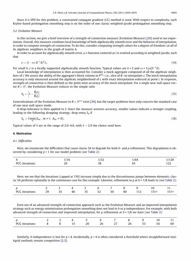
Here, we enumerate the difficulties that cause classic SA to degrade for both h- and p-refinement. This degradation is ob-served by considering p = 1 for our model problem (see Table 2):
h 1/16 1/32 1/64 1/128PCG iterations: 26 38 65 122
Here, we see that the iterations (capped at 150) increase simply due to the discontinuous jumps between elements; clas-sic SA performs optimally in the continuous case for this example. Likewise, refinement in p at h = 1/8 leads to (see Table 2):
Even use of an advanced strength-of-connection approach such as the Evolution Measure and an improved interpolationstrategy such as energy-minimization prolongation smoothing does not lead to h or p independence. For example, with bothadvanced strength-of-connection and improved interpolation, for p refinement at h = 1/8 we have (see Table 2):
Similarly, h-independence is lost for p > 4. Incidentally, p = 4 is often considered a threshold where straightforward mul-tigrid methods remain competitive [2,3].
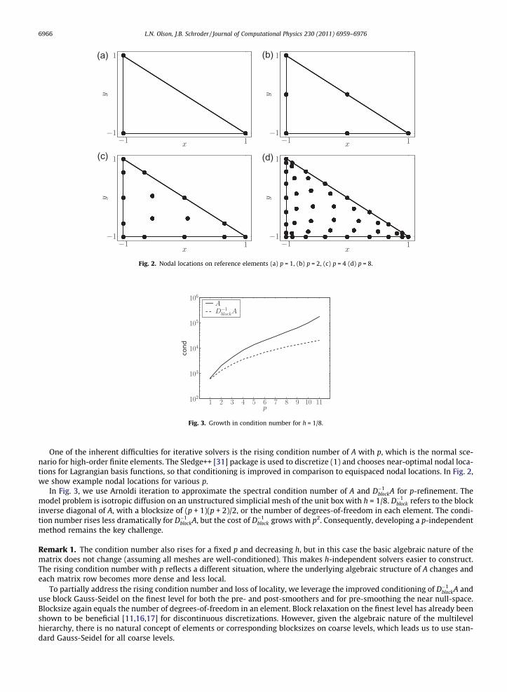
One of the inherent difficulties for iterative solvers is the rising condition number of A with p, which is the normal sce-nario for high-order finite elements. The Sledge++ [31] package is used to discretize (1) and chooses near-optimal nodal loca-tions for Lagrangian basis functions, so that conditioning is improved in comparison to equispaced nodal locations. In Fig. 2,we show example nodal locations for various p.
In Fig. 3, we use Arnoldi iteration to approximate the spectral condition number of A and D!1blockA for p-refinement. The
model problem is isotropic diffusion on an unstructured simplicial mesh of the unit box with h = 1/8. D!1block refers to the block
inverse diagonal of A, with a blocksize of (p + 1)(p + 2)/2, or the number of degrees-of-freedom in each element. The condi-tion number rises less dramatically for D!1
blockA, but the cost of D!1block grows with p2. Consequently, developing a p-independent
method remains the key challenge.
Remark 1. The condition number also rises for a fixed p and decreasing h, but in this case the basic algebraic nature of thematrix does not change (assuming all meshes are well-conditioned). This makes h-independent solvers easier to construct.The rising condition number with p reflects a different situation, where the underlying algebraic structure of A changes andeach matrix row becomes more dense and less local.
To partially address the rising condition number and loss of locality, we leverage the improved conditioning of D!1blockA and
use block Gauss-Seidel on the finest level for both the pre- and post-smoothers and for pre-smoothing the near null-space.Blocksize again equals the number of degrees-of-freedom in an element. Block relaxation on the finest level has already beenshown to be beneficial [11,16,17] for discontinuous discretizations. However, given the algebraic nature of the multilevelhierarchy, there is no natural concept of elements or corresponding blocksizes on coarse levels, which leads us to use stan-dard Gauss-Seidel for all coarse levels.
(a) (b)
(d)(c)
Fig. 2. Nodal locations on reference elements (a) p = 1, (b) p = 2, (c) p = 4 (d) p = 8.
Additionally, the number of iterations for energy-minimization prolongation smoothing and of time steps k taken by theEvolution Measure needs to rise with p. However, there is a bottleneck with the Evolution Measure and k, since the largestcomputationally feasible value is k = 4 and this still results in a strength measure that is of the same complexity as comput-ing A2. For some problems, even squaring the matrix is too expensive. Thus, larger values of k results in intolerable complex-ity and limited value.
4.2. Conforming aggregation
The main issue not addressed so far is aggregation in the high-order discontinuous setting, for which no standard methodexists. One clear difference for discontinuous Galerkin discretizations, in comparison to standard discretizations, is that eachelement has a distinct set of degrees-of-freedom, leading to multiple degrees-of-freedom at each nodal location on sharedelement boundaries. A similar problem occurs for PDE systems where multiple variables exist at the same spatial location.The classic SA approach to this issue is supernodes [32], which are designed to aggregate vector problems with multiple vari-ables at the same spatial location. The supernode approach yields an aggregation in two stages at the finest level. In the firststage, supernodes are formed by aggregating degrees-of-freedom at the same spatial location together. The second stagethen aggregates strongly connected supernodes together.
A supernode-like approach here corresponds to conforming aggregation on the finest level, wherein all degrees-of-freedom at the same spatial location are collected. All other degrees-of-freedom are injected as singleton aggregates tothe next level. We label this conforming aggregation due to its similarity with a C0-projection. To accomplish this, onlythe strength matrix S must be changed on the finest level. Moreover, no prolongation smoothing is required on the finestlevel, so that the tentative P = P(0).
A conforming step is well-motivated. Degrees-of-freedom at the same spatial location have similar solution values, thusconstant-based interpolation remains tractable. Additionally, a conforming step allows SA to separate decisions about twoentirely different types of algebraic connections into two distinct phases—i.e., connections between degrees-of-freedom atthe same spatial location are considered only on the finest level, and longer-range connections are considered only on coarselevels. Lastly considering the motivating example of isotropic diffusion, we know that degrees-of-freedom close togetherspatially should be aggregated together. Hence, degrees-of-freedom at the same location that are also algebraic neighborsare in a unique class of exceptionally strong connections.
In order to better visualize a conforming aggregation step, Fig. 4 shows a sample conforming aggregation on level 0. Theblack triangles are the element boundaries and each element is shrunk towards its barycenter in order to depict the discon-tinuous nature of the discretization. The colored polygons and lines represent aggregates.
4.3. Distance-based aggregation
Building on the idea of conforming aggregation and restricting ourselves to isotropic problems, we next consider a dis-tance-based strength-of-connection measure. For isotropic diffusion on an isotropic mesh, where algebraically smooth erroris slowly varying in all directions, aggregates should be evenly sized and convex in shape. Thus, a distance-based measure isappropriate. Since we (and classic SA) assume access to the underlying mesh points, we define a distance-based measure.The weak neighbors for a degree-of-freedom i are those degrees-of-freedom whose distance from i is larger than twicethe distance of the nearest neighbor.
This approach is computationally inexpensive, because the strength matrix S essentially becomes A, with A’s entries re-placed with distance values. Entries in S are then dropped according to the criteria above. Aggregation then proceeds as nor-mal, making the computation of S on the finest level the only algorithmic modification of this approach. Advantageously, useof a distance-based measure on the finest level results in a lower operator complexity than using only a conforming step onthe finest level. This is because the distance-based measure coarsens more aggressively by combining both a conformingaggregation step and aggregation of nearby degrees-of-freedom into the fine level aggregation phase.
Fig. 4. Example of conforming aggregation in the interior of a domain (a) p = 5 Conforming Aggregation, (b) p = 7 Conforming Aggregation.
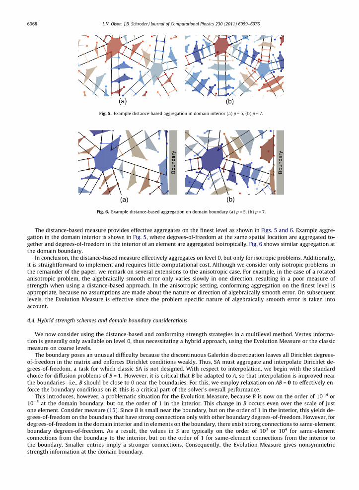
The distance-based measure provides effective aggregates on the finest level as shown in Figs. 5 and 6. Example aggre-gation in the domain interior is shown in Fig. 5, where degrees-of-freedom at the same spatial location are aggregated to-gether and degrees-of-freedom in the interior of an element are aggregated isotropically. Fig. 6 shows similar aggregation atthe domain boundary.
In conclusion, the distance-based measure effectively aggregates on level 0, but only for isotropic problems. Additionally,it is straightforward to implement and requires little computational cost. Although we consider only isotropic problems inthe remainder of the paper, we remark on several extensions to the anisotropic case. For example, in the case of a rotatedanisotropic problem, the algebraically smooth error only varies slowly in one direction, resulting in a poor measure ofstrength when using a distance-based approach. In the anisotropic setting, conforming aggregation on the finest level isappropriate, because no assumptions are made about the nature or direction of algebraically smooth error. On subsequentlevels, the Evolution Measure is effective since the problem specific nature of algebraically smooth error is taken intoaccount.
4.4. Hybrid strength schemes and domain boundary considerations
We now consider using the distance-based and conforming strength strategies in a multilevel method. Vertex informa-tion is generally only available on level 0, thus necessitating a hybrid approach, using the Evolution Measure or the classicmeasure on coarse levels.
The boundary poses an unusual difficulty because the discontinuous Galerkin discretization leaves all Dirichlet degrees-of-freedom in the matrix and enforces Dirichlet conditions weakly. Thus, SA must aggregate and interpolate Dirichlet de-grees-of-freedom, a task for which classic SA is not designed. With respect to interpolation, we begin with the standardchoice for diffusion problems of B = 1. However, it is critical that B be adapted to A, so that interpolation is improved nearthe boundaries—i.e., B should be close to 0 near the boundaries. For this, we employ relaxation on AB = 0 to effectively en-force the boundary conditions on B; this is a critical part of the solver’s overall performance.
This introduces, however, a problematic situation for the Evolution Measure, because B is now on the order of 10!4 or10!5 at the domain boundary, but on the order of 1 in the interior. This change in B occurs even over the scale of justone element. Consider measure (15). Since B is small near the boundary, but on the order of 1 in the interior, this yields de-grees-of-freedom on the boundary that have strong connections only with other boundary degrees-of-freedom. However, fordegrees-of-freedom in the domain interior and in elements on the boundary, there exist strong connections to same-elementboundary degrees-of-freedom. As a result, the values in S are typically on the order of 103 or 104 for same-elementconnections from the boundary to the interior, but on the order of 1 for same-element connections from the interior tothe boundary. Smaller entries imply a stronger connections. Consequently, the Evolution Measure gives nonsymmetricstrength information at the domain boundary.
Fig. 5. Example distance-based aggregation in domain interior (a) p = 5, (b) p = 7.
Fig. 6. Example distance-based aggregation on domain boundary (a) p = 5, (b) p = 7.
This nonsymmetric strength information is correct, despite the fact that the matrix A is symmetric and based on an ellip-tic PDE. Degrees-of-freedom near the Dirichlet boundary are strongly connected to the degrees-of-freedom on the Dirichletboundary, but not vice-versa. Since strength information communicates the accuracy of interpolation for algebraicallysmooth error between two degrees-of-freedom, we consider the desired action of interpolation in order to highlight this sub-tle issue. Interpolation from the interior to the Dirichlet boundary is appropriate, because interpolation targets zero bound-ary values with small interpolation weights. However, interpolation from the Dirichlet boundary to the domain interior isinaccurate because the solution value on the boundary, which is approximately 0, contains no useful information about alge-braically smooth error in the interior.
This is problematic because each aggregate is represented by a single coarse grid variable, and this coarse grid variable(and corresponding coarse grid matrix row), must accurately represent algebraically smooth error for the entire aggregateon the fine grid. This is achieved by using symmetric strength information. For example, a strong connection between iand j indicates that algebraically smooth error can be accurately interpolated from i to j and from j to i.
Therefore, we propose to symmetrize the Evolution Measure [29], so that the update S S + ST occurs before the drop-tolerance is applied. This change greatly improves aggregation at the boundary and we use it in our experiments; if theunsymmetrized version is used, performance deteriorates significantly.
Fig. 7. Example Level 1 Evolution Measure aggregation on domain boundary, conforming aggregation used on level 0 (a) p = 5, Symmetrized S, (b) p = 7,Symmetrized S.
Fig. 8. Example Level 1 Evolution Measure aggregation on domain boundary, conforming aggregation used on level 0 (a) p = 5, Unsymmetrized S, (b) p = 7,Unsymmetrized S.
Fig. 9. Example Level 1 Evolution Measure aggregation in domain interior, conforming aggregation used on level 0 (a) p = 5, Symmetrized orUnsymmetrized S, (b) p = 7, Symmetrized or Unsymmetrized S.
To illustrate the importance of symmetrizing S, Figs. 7 and 8 depict aggregation at the domain boundary for a symme-trized and unsymmetrized S, respectively. The aggregates are projected from level 1, because a conforming step is usedon the finest level. In Fig. 7, aggregates are sensible with boundary degrees-of-freedom aggregated together and degrees-of-freedom in the interior aggregated isotropically. If the Evolution Measure is not modified, then very poor aggregation oc-curs, yielding irregular and oversized aggregates near the boundary as depicted in Fig. 8. The result is that SA performancesuffers.
In the domain interior, symmetric and nonsymmetric S yield similar results. Sample aggregation is depicted in Fig. 9,where degrees-of-freedom at the same spatial location are aggregated together and degrees-of-freedom in the interior ofan element are aggregated isotropically. The difficulty posed by using a nonsymmetric S has not been observed for problems
Fig. 10. Example stand-alone Evolution Measure aggregation on domain boundary (a) p = 5, Level 0, (b) p = 7, Level 0, (c) p = 5, Level 1, (d) p = 7, Level 1.
Fig. 11. Example stand-alone Evolution Measure aggregation in domain interior (a) p = 5, Level 0, (b) p = 7, Level 0, (c) p = 5, Level 1, (d) p = 7, Level 1.
where continuous Galerkin discretizations are used. The critical difference is that no boundary degrees-of-freedom areexplicitly represented in the matrix.
4.5. Stand-alone Evolution Measure aggregation
Stand-alone use of the Evolution Measure on all levels of the hierarchy also produces an effective SA solver, particularly atlow to moderate p. We therefore visualize how the stand-alone Evolution Measure aggregates. We show only aggregation forthe symmetrized Evolution Measure, as the unsymmetrized version again has very poor aggregation near the boundary.Figs. 10 and 11 show example aggregation on levels 0 and 1 on the domain boundary and in the domain interior, respec-tively. The Evolution Measure aggregates as expected in both cases.
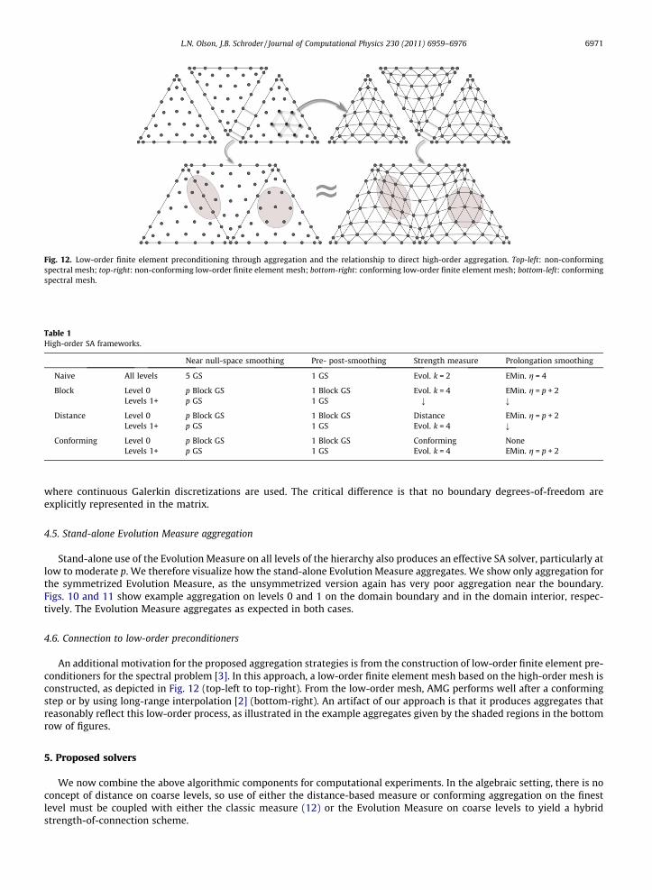
4.6. Connection to low-order preconditioners
An additional motivation for the proposed aggregation strategies is from the construction of low-order finite element pre-conditioners for the spectral problem [3]. In this approach, a low-order finite element mesh based on the high-order mesh isconstructed, as depicted in Fig. 12 (top-left to top-right). From the low-order mesh, AMG performs well after a conformingstep or by using long-range interpolation [2] (bottom-right). An artifact of our approach is that it produces aggregates thatreasonably reflect this low-order process, as illustrated in the example aggregates given by the shaded regions in the bottomrow of figures.
5. Proposed solvers
We now combine the above algorithmic components for computational experiments. In the algebraic setting, there is noconcept of distance on coarse levels, so use of either the distance-based measure or conforming aggregation on the finestlevel must be coupled with either the classic measure (12) or the Evolution Measure on coarse levels to yield a hybridstrength-of-connection scheme.
Fig. 12. Low-order finite element preconditioning through aggregation and the relationship to direct high-order aggregation. Top-left: non-conformingspectral mesh; top-right: non-conforming low-order finite element mesh; bottom-right: conforming low-order finite element mesh; bottom-left: conformingspectral mesh.
Table 1High-order SA frameworks.
Near null-space smoothing Pre- post-smoothing Strength measure Prolongation smoothing
Naive All levels 5 GS 1 GS Evol. k = 2 EMin. g = 4
Block Level 0 p Block GS 1 Block GS Evol. k = 4 EMin. g = p + 2Levels 1+ p GS 1 GS ; ;
Distance Level 0 p Block GS 1 Block GS Distance EMin. g = p + 2Levels 1+ p GS 1 GS Evol. k = 4 ;
Conforming Level 0 p Block GS 1 Block GS Conforming NoneLevels 1+ p GS 1 GS Evol. k = 4 EMin. g = p + 2
Table 1 outlines the proposed solver components. The conforming and distance-based frameworks are the most advancedbecause of the special fine level strength-of-connection strategies discussed above. In our numerical experiments, we useGauss-Seidel smoothing (denoted ‘‘j GS’’ for j sweeps), along with the Evolution Measure (denoted ‘‘Evol.’’ with k sweeps)and energy-minimization prolongation smoothing to improve interpolation (denoted ‘‘EMin.’’ with g iterations). We labelthe classic use of SA as the ‘‘Naive’’ method, while ‘‘Block’’ refers to the use of D!1
block. The hybrid strength frameworks, ‘‘Con-forming’’ and ‘‘Distance’’, correspond to the block framework enhanced on the finest level with conforming aggregation andthe distance-based strength measure, respectively.
A numerical study in h and p is done. The LDG, IP and Brezzi et al. methods are used to discretize (1) with the strong-weakform. Our experiments with uniform Dirichlet boundary conditions and mixtures of Neumann and Dirichlet yielded no qual-itative difference in performance, so we reproduce results primarily for the Dirichlet case. Using Sledge++, matrices are gen-erated for non-nested unstructured simplicial meshes of the unit box in 2D for decreasing h and various p. W(1,1)-cyclesprecondition CG to a relative residual tolerance of 10!8, with the number of iterations capped at 150. W(1,1)-cycles are usedbecause they exhibit grid independent behavior in cases that V-cycles do not. The result is that W-cycles give lower cost perdigit-of-accuracy than V-cycles. The coarsest grid is 100 degrees-of-freedom. The test problem is a zero initial guess and arandom right-hand side.
Tables 2 and 3 depict the performance for the four different SA frameworks in Table 1. We restrict ourselves to showingresults for the LDG method, because the results for the IP and Brezzi et al. methods were qualitatively no different. For thepurposes of comparison, we also experiment with weighted-Jacobi prolongation smoothing and the classic strengthmeasure.
The classic measure is not well-suited to this complex algebraic setting of non-M-matrices, but h = 0.1 is empirically a fairchoice for general p and is used here. Additionally, the use of filtered-matrix prolongation smoothing for classic weighted-Jacobi was critical for controlling complexity—e.g., an operator-complexity of 9 versus 2.25. Filtered-matrix prolongationsmoothing essentially lumps weak connections on the diagonal of A for only the prolongation smoothing step. The sparsity
pattern constraint for energy-minimization prolongation smoothing accomplishes the same goal of controlling complexity.In general, operator complexities are in the range 2.25–2.50 for all frameworks except the conforming framework, which hasoperator complexities in the range 2.60–3.20.
Table 2 gives results for the naive framework from Table 1. It is observed that the combination of energy-minimizationprolongation smoothing and the Evolution Measure provides h-independence until p = 6 and p-independence until p = 4. Noother method in Table 2 is competitive for p > 1 with the combination of energy-minimization prolongation smoothing andthe Evolution Measure.
Table 2 also gives results for the block methods framework from Table 1, which generally yields better PCG iterationcounts than the naive framework for p > 6. Combination of energy-minimization prolongation smoothing and the EvolutionMeasure provides h-independence until p = 7, with a slow degradation for increasing h and fixed p thereafter . There isp-independence again until p = 4. No other method in Table 2 is competitive for p > 1 with the combination of energy-minimization prolongation smoothing and the Evolution Measure.
Table 3 gives results for the ‘‘Distance’’ framework from Table 1. The hybrid strength schemes are referred to as ‘‘Dist.–Classic’’ and ‘‘Dist.–Evol.’’ and correspond to the use of the distance-based measure on the finest level and the classic mea-sure and the Evolution Measure on coarse levels, respectively. Importantly, h = 0.1 for the classic measure is detrimental toperformance for the hybrid strength schemes, but h = 0.0 performed well and is used here for the two hybrid schemes. De-spite tuning h for the classic measure, the ‘‘Dist.–Evol.’’ scheme exhibits superior performance beyond p = 2. In particular, thecombination of energy-minimization prolongation smoothing and ‘‘Dist.–Evol.’’ yields h-independence until p = 9, with asmall degradation for increasing h at p = 10 and 11. Additionally, p-independence is extended until p = 6. Degradation forincreasing p and fixed h is thereafter slow.
Table 3 also gives results for the ‘‘Conforming’’ framework from Table 1. The hybrid strength schemes are referred to as‘‘Conf.–Classic’’ and ‘‘Conf.–Evol.’’ and correspond to the use of conforming aggregation on the finest level and the classicmeasure and the Evolution Measure on coarse levels, respectively. The results are largely similar to the distance framework,with combination of ‘‘Conf.–Evol.’’ and energy-minimization prolongation smoothing providing the most robust method. Theone downside to using conforming aggregation on the finest level is that operator complexities are higher because this is theleast aggressive coarsening approach.
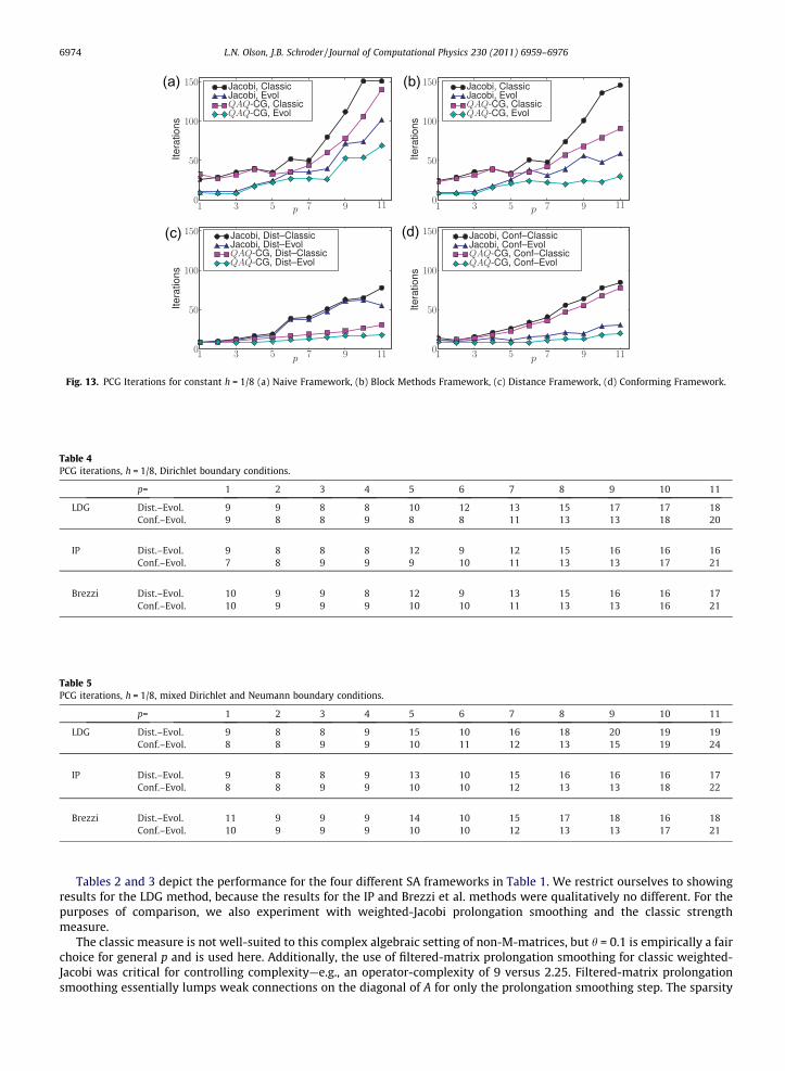
In order to better visualize how iterations increase with p, Fig. 13 depicts plots of p versus PCG iterations, for a constanth = 1/8. The data is taken from Tables 2 and 3. This is the only h value shared by all p values. The two hybrid strength schemesproduce the solvers with behavior closest to p-independence.
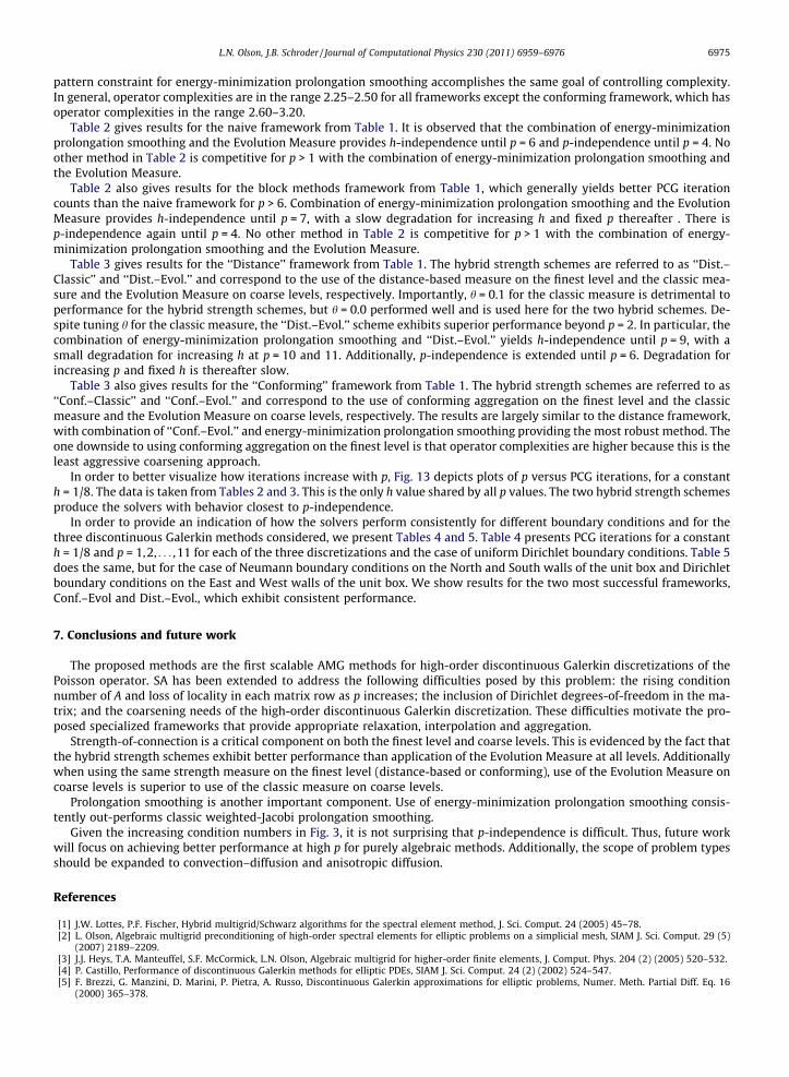
In order to provide an indication of how the solvers perform consistently for different boundary conditions and for thethree discontinuous Galerkin methods considered, we present Tables 4 and 5. Table 4 presents PCG iterations for a constanth = 1/8 and p = 1,2, . . . ,11 for each of the three discretizations and the case of uniform Dirichlet boundary conditions. Table 5does the same, but for the case of Neumann boundary conditions on the North and South walls of the unit box and Dirichletboundary conditions on the East and West walls of the unit box. We show results for the two most successful frameworks,Conf.–Evol and Dist.–Evol., which exhibit consistent performance.
7. Conclusions and future work
The proposed methods are the first scalable AMG methods for high-order discontinuous Galerkin discretizations of thePoisson operator. SA has been extended to address the following difficulties posed by this problem: the rising conditionnumber of A and loss of locality in each matrix row as p increases; the inclusion of Dirichlet degrees-of-freedom in the ma-trix; and the coarsening needs of the high-order discontinuous Galerkin discretization. These difficulties motivate the pro-posed specialized frameworks that provide appropriate relaxation, interpolation and aggregation.
Strength-of-connection is a critical component on both the finest level and coarse levels. This is evidenced by the fact thatthe hybrid strength schemes exhibit better performance than application of the Evolution Measure at all levels. Additionallywhen using the same strength measure on the finest level (distance-based or conforming), use of the Evolution Measure oncoarse levels is superior to use of the classic measure on coarse levels.
Prolongation smoothing is another important component. Use of energy-minimization prolongation smoothing consis-tently out-performs classic weighted-Jacobi prolongation smoothing.
Given the increasing condition numbers in Fig. 3, it is not surprising that p-independence is difficult. Thus, future workwill focus on achieving better performance at high p for purely algebraic methods. Additionally, the scope of problem typesshould be expanded to convection–diffusion and anisotropic diffusion.
References
[1] J.W. Lottes, P.F. Fischer, Hybrid multigrid/Schwarz algorithms for the spectral element method, J. Sci. Comput. 24 (2005) 45–78.[2] L. Olson, Algebraic multigrid preconditioning of high-order spectral elements for elliptic problems on a simplicial mesh, SIAM J. Sci. Comput. 29 (5)
(2007) 2189–2209.[3] J.J. Heys, T.A. Manteuffel, S.F. McCormick, L.N. Olson, Algebraic multigrid for higher-order finite elements, J. Comput. Phys. 204 (2) (2005) 520–532.[4] P. Castillo, Performance of discontinuous Galerkin methods for elliptic PDEs, SIAM J. Sci. Comput. 24 (2) (2002) 524–547.[5] F. Brezzi, G. Manzini, D. Marini, P. Pietra, A. Russo, Discontinuous Galerkin approximations for elliptic problems, Numer. Meth. Partial Diff. Eq. 16
[6] D.N. Arnold, F. Brezzi, B. Cockurn, L.D. Marini, Unified analysis of discontinuous Galerkin methods for elliptic problems, SIAM J. Numer. Anal. 39 (2002)1749–1779.
[7] B. Cockburn, J. Gopalakrishnan, R. Lazarov, Unified hybridization of discontinuous Galerkin, mixed, and continuous Galerkin methods for second orderelliptic problems, SIAM J. Numer. Anal. 47 (2) (2009) 1319–1365.
[8] N.C. Nguyen, J. Peraire, B. Cockburn, A hybridizable discontinuous Galerkin method for stokes flow, Comput. Methods Appl. Mech. Eng. 199 (9-12)(2010) 582–597.
[9] Y. Jeon, E.. Park, A hybrid discontinuous Galerkin method for elliptic problems, SIAM J. Numer. Anal. 48 (5) (2010) 1968–1983.[10] G. Kanschat, Preconditioning methods for local discontinuous Galerkin discretizations, SIAM J. Sci. Comput. 25 (3) (2003) 815–831.[11] G. Kanschat, Robust smoothers for high-order discontinuous Galerkin discretizations of advection–diffusion problems, J. Comput. Appl. Math. 218 (1)
(2008) 53–60 (special Issue: Finite Element Methods in Engineering and Science (FEMTEC 2006)).[12] H. Atkins, B. Helenbrook, Application of p-multigrid to discontinuous Galerkin formulations of the Poisson operator, AIAA J. 44 (3) (2005) 566–575.[13] K.J. Fidkowski, T.A. Oliver, J. Lu, D.L. Darmofal, p-multigrid solution of high-order discontinuous Galerkin discretizations of the compressible Navier–
Stokes equations, J. Comput. Phys. 207 (1) (2005) 92–113.[14] V.A. Dobrev, R.D. Lazarov, P.S. Vassilevski, L.T. Zikatanov, Two-level preconditioning of discontinuous Galerkin approximations of second-order elliptic
equations, Numer. Linear Algebra Appl. 13 (9) (2006) 753–770.[15] J. Gopalakrishnan, G. Kanschat, A multilevel discontinuous Galerkin method, Numer. Math. 95 (3) (2003) 527–550.[16] P.W. Hemker, W. Hoffmann, M.H. v. Raalte, Two-level Fourier analysis of a multigrid approach for discontinuous Galerkin discretizations, SIAM J. Sci.
Comput. 25 (3) (2003) 1018–1041.[17] F. Prill, M. Lukácová-Medvidová, R. Hartmann, Smoothed aggregation multigrid for the discontinuous Galerkin method, SIAM J. Sci. Comput. 31 (5)
(2009) 3503–3528.[18] B. Cockburn, C.-W. Shu, The local discontinuous Galerkin method for time-dependent convection–diffusion systems, SIAM J. Numer. Anal. 35 (6) (1998)
2440–2463.[19] J.J. Douglas, T. Dupont, Interior penalty procedures for elliptic and parabolic Galerkin methods, in: Computing Methods in Applied Sciences, Lecture
Notes in Physics, vol. 58, Springer, Berlin, 1976, pp. 207–216.[20] F. Brezzi, G. Manzini, D. Marini, P. Pietra, A. Russo, Discontinuous finite elements for diffusion problems, in: in Atti Convegno in onore di F. Brioschi
(Milan, 1997), Instituto Lombardo, Accademia di Scienze e Lettere, Italy, 1999, pp. 197–217.[21] P. Castillo, B. Cockurn, I. Perugia, D. Schötzau, An a priori error analysis of the local discontinuous Galerkin method for elliptic problems, SIAM J. Numer.
Anal. 38 (2000) 1676–1706.[22] B. Cockurn, G. Kanschat, I. Perugia, D. Schötzau, Superconvergence of the local discontinuous Galerkin method for elliptic problems on Cartesian grids,
SIAM J. Numer. Anal. 39 (2001) 264–285.[23] J. Hesthaven, T. Warburton, Nodal discontinuous Galerkin methods: algorithms, analysis, and applications, Texts in applied mathematics, vol. 54,
Springer, Berlin, 2008.[24] S.F. McCormick, J.W. Ruge, Multigrid methods for variational problems, SIAM J. Numer. Anal. 19 (5) (1982) 924–929.[25] M. Brezina, R. Falgout, S. MacLachlan, T. Manteuffel, S. McCormick, J. Ruge, Adaptive smoothed aggregation (aSA) multigrid, SIAM Rev. 47 (2) (2005)
317–346.[26] M. Brezina, T. Manteuffel, S. Mccormick, J. Ruge, G. Sanders, Towards adaptive smoothed aggregation (aSA) for nonsymmetric problems, SIAM J. Sci.
Comput.[27] P. Vanek, J. Mandel, M. Brezina, Algebraic multigrid based on smoothed aggregation for second and fourth order problems, Computing 56 (1996) 179–
196.[28] J. Brannick, M. Brezina, S. MacLachlan, T. Manteuffel, S. McCormick, J. Ruge, An energy-based AMG coarsening strategy, Numer. Linear Algebra Appl. 13
(2-3) (2006) 133–148.[29] L.N. Olson, J.B. Schroder, R.S. Tuminaro, A new perspective on strength measures in algebraic multigrid, Numer. Linear Algebra Appl. 17 (4) (2010) 713–
733.[30] L.N. Olson, J.B. Schroder, R.S. Tuminaro, A general interpolation strategy for algebraic multigrid using energy-minimization, SIAM J. Sci. Comput.
Submitted.[31] T. Warburton, J. Hesthaven, L. Wilcox, Sledge++ users’ guide (2006). <http://www.caam.rice.edu/timwar/TimWarburton/Sledge++.html>.[32] P. Vanek, M. Brezina, J. Mandel, Convergence of algebraic multigrid based on smoothed aggregation, Numer. Math. 88 (3) (2001) 559–579.