Journal of Hydrology 522 (2015) 203–210

Contents lists available at ScienceDirect

Journal of Hydrology

journal homepage: www.elsevier .com/ locate / jhydrol

A new approach for continuous estimation of baseflow using discretewater quality data: Method description and comparison with baseflowestimates from two existing approaches

http://dx.doi.org/10.1016/j.jhydrol.2014.12.0390022-1694/Published by Elsevier B.V.

⇑ Corresponding author. Tel.: +1 801 908 5065.E-mail address: mamiller@usgs.gov (M.P. Miller).

Matthew P. Miller a,⇑, Henry M. Johnson b, David D. Susong a, David M. Wolock c

a U.S. Geological Survey, Utah Water Science Center, 2329 Orton Circle, Salt Lake City, UT 84119, USAb U.S. Geological Survey, Oregon Water Science Center, 2130 SW 5[th] Ave, Portland, OR 97201, USAc U.S. Geological Survey, Kansas Water Science Center, 4821 Quail Crest Place, Lawrence, KS 66049, USA

a r t i c l e i n f o

Article history:Received 6 August 2014Received in revised form 12 December 2014Accepted 15 December 2014Available online 24 December 2014This manuscript was handled by CorradoCorradini, Editor-in-Chief, with theassistance of Rao S. Govindaraju, AssociateEditor

Keywords:BaseflowConductivity mass balanceSpecific conductanceHydrograph separationGroundwater

s u m m a r y

Understanding how watershed characteristics and climate influence the baseflow component of streamdischarge is a topic of interest to both the scientific and water management communities. Therefore, thedevelopment of baseflow estimation methods is a topic of active research. Previous studies have demon-strated that graphical hydrograph separation (GHS) and conductivity mass balance (CMB) methods canbe applied to stream discharge data to estimate daily baseflow. While CMB is generally considered tobe a more objective approach than GHS, its application across broad spatial scales is limited by a lackof high frequency specific conductance (SC) data. We propose a new method that uses discrete SC data,which are widely available, to estimate baseflow at a daily time step using the CMB method. The pro-posed approach involves the development of regression models that relate discrete SC concentrationsto stream discharge and time. Regression-derived CMB baseflow estimates were more similar to baseflowestimates obtained using a CMB approach with measured high frequency SC data than were the GHSbaseflow estimates at twelve snowmelt dominated streams and rivers. There was a near perfect fitbetween the regression-derived and measured CMB baseflow estimates at sites where the regressionmodels were able to accurately predict daily SC concentrations. We propose that the regression-derivedapproach could be applied to estimate baseflow at large numbers of sites, thereby enabling futureinvestigations of watershed and climatic characteristics that influence the baseflow component of streamdischarge across large spatial scales.

Published by Elsevier B.V.

1. Introduction

Scientists and managers are often interested in identifying howwatershed characteristics (e.g. geology, land use, soil type, etc.) andclimatic conditions influence baseflow discharge to streams.Addressing such processes requires quantitative estimates ofbaseflow discharge across a gradient of watershed types. Thedevelopment of quantitative methods for baseflow estimation isalso necessary to understand water budgets (Stewart et al.,2007), estimate groundwater discharge (Arnold and Allen, 1999)and associated effects on stream temperature (Hill et al., 2013),and address questions of the vulnerability and response of thewater cycle to natural and human-induced change in environmen-tal conditions, such as stream vulnerability to legacy nutrients(Tesoriero et al., 2013). Given the importance of baseflow, many

methods have been used to quantify the baseflow component ofstream discharge beginning with Boussinesq (1877).

Approaches for baseflow estimation can be grouped into twogeneral categories: graphical hydrograph separation (GHS) meth-ods, which rely on stream discharge data alone, and tracer massbalance (MB) methods, which rely on chemical constituents inthe stream, stream discharge, and the streamflow end-memberconstituent concentrations (runoff and baseflow). Many differentapproaches for GHS exist, including recession curve methods anddigital filter methods. Recession curve methods are generally con-sidered more objective than digital filter methods because theyprovide an assumed integrated signal of basin hydrologic and geo-logic characteristics through identification of a linear recession-constant based on the falling limb of the hydrograph (Barnes,1939; Hall, 1968; Gardner et al., 2010). However, the ability ofrecession curve methods to quantify groundwater discharge tostreams has been questioned because of the accuracy of themethod assumptions (Halford and Mayer, 2000). Digital filter

204 M.P. Miller et al. / Journal of Hydrology 522 (2015) 203–210

methods either filter high frequency (assumed to be surface runoff)signals from low frequency (assumed to be baseflow) signals(Nathan and McMahon, 1990), or identify and connect successiveminima on a stream hydrograph, and define baseflow as the lineconnecting the minima (Wahl and Wahl, 1988; Wolock, 2003).The definitions of basin-specific parameters used in these methodsare generally subjective and not based on hydrologic processes(Stewart et al., 2007).

It has been suggested that MB methods for baseflow estimationare more objective than GHS because measured stream water con-centrations, and either measured or estimated end-member con-centrations, are related to physical and chemical processes andflow paths in the basin (Stewart et al., 2007; Zhang et al., 2013).One type of MB method that is commonly applied is the conductiv-ity mass balance (CMB) method, which uses specific conductance(SC) as a chemical tracer for hydrograph separation. One advantageof CMB over other types of MB methods is that SC is relatively easyand inexpensive to measure. Additionally, high frequency SC mea-surements can be obtained using in-situ SC probes. High frequencySC data and CMB methods have been used to estimate baseflowacross gradients of watershed size and land use settings (Covinoand McGlynn, 2007; Miller et al., 2014; Pellerin et al., 2007;Stewart et al., 2007).

While CMB methods are generally considered to be more objec-tive than GHS methods, their application is limited by the fact thatthey require high frequency SC records that are not always widelyavailable over long time periods or spanning large numbers ofwatersheds. Multiple studies have developed methods to calibrateGHS estimates of baseflow to CMB estimates of baseflow (Lott andStewart, 2013; Stewart et al., 2007; Zhang et al., 2013). Once cali-brated at a specific stream location, and assuming that the end-member SC concentrations are constant over time, the GHS meth-ods can be applied to long term stream discharge records at thatlocation to estimate baseflow for time periods that span dateranges greater than those for which high frequency SC data areavailable. Li et al. (2014) showed that as little as six months of highfrequency SC data can be used to calibrate a recursive digital filtermodel, which can then be applied to long term stream dischargerecords to estimate baseflow. This approach overcomes the CMBlimitations associated with the lack of long-term SC records, butis only applicable at sites that have high frequency SC data avail-able for GHS calibration. Unfortunately, high frequency SC dataare not generally available at large numbers of sites within a givenregion. Therefore, the use of CMB, or calibration of GHS to CMB, toestimate baseflow and quantify environmental drivers of baseflowdischarge across broad spatial scales is limited.

We propose that discrete SC concentration data and daily meandischarge data, which are frequently available at large numbers ofsites, can be used with a CMB method to estimate baseflow at a dailytime-step for the period of record of discharge data, thereby increas-ing the number of sites at which CMB can be used to estimate base-flow. The proposed approach involves the calibration of site-specificregression models that relate discrete SC concentrations to streamdischarge and time to predict daily SC concentrations, and subse-quently regression-derived CMB baseflow estimates, for the periodof stream discharge record. A similar regression approach has beenused to estimate water quality data, and subsequently groundwaterdischarge to a tropical stream for time periods when no water qual-ity data exist (Genereux et al., 2005), but has not been applied to anumber of sites and compared with other baseflow estimates fromthe same sites. The objective of this study is to test the proposedapproach by comparing the regression-derived baseflow estimateswith CMB baseflow estimates calculated using measured highfrequency SC data (assumed to be the most objective estimates ofbaseflow) at twelve snowmelt dominated streams and rivers inthe Upper Colorado River Basin (UCRB). As previously reported by

Miller et al. (2014), CMB methods are well suited for estimatingbaseflow in snowmelt dominated watersheds. Baseflow estimatescalculated using a commonly applied GHS model were also com-pared with measured CMB baseflow estimates.

2. Materials and methods

2.1. Site description

The UCRB is a heavily regulated watershed located in the wes-tern United States and drains an area of 294,000 km2. The headwa-ters are high elevation catchments in the Rocky Mountains and thedownstream end of the UCRB is located at Page, AZ, downstream ofLake Powell on the Colorado River (Fig. 1). Miller et al. (2014) esti-mated baseflow discharge at a daily time step for the period ofrecord at fourteen sites draining large watersheds in the UCRBcharacteristic of snowmelt dominated hydrology using measuredhigh frequency SC data with a CMB approach. As part of this pro-cess sites were screened for impacts due to anthropogenic activi-ties. Twelve of these fourteen sites are included in the presentmethods comparison (Fig. 1, Table 1). Two of the fourteen sites –The Gunnison River at Delta, CO and The Uncompahgre River atColona, CO – are not included in the present study because theshort periods of record for which high frequency SC data are avail-able at these sites resulted in a limited discrete SC data set that wasnot adequate for development of regression models to estimatedaily SC concentrations. Drainage areas range from 1500 km2 atPLAT to 62,000 km2 at CO3. Average baseflow estimates range from1.0 ± 1.2 m3/s to 103 ± 9.6 m3/s, and the fraction of total stream-flow estimated to be baseflow ranges from 11% to 59% (Table 1).Detailed site descriptions for these twelve locations are availablein Miller et al. (2014).

2.2. Data sources

Daily mean discharge, daily mean SC, and discrete SC data wereobtained from the U.S. Geological Survey (USGS) National WaterInformation System (NWIS) database. The date ranges for whichdata were acquired were limited to date ranges for which bothdaily mean discharge and daily mean SC data were available. Peri-ods of records ranged from 3 to 37 years and the number of dis-crete samples used in regression model calibration (forestimation of daily regression-derived SC concentrations) rangedfrom 17 to 623 (Table 1). Detailed information regarding the peri-ods of record, average discharge, and average SC at each site areavailable in Miller et al. (2014).

2.3. Regression-derived daily SC

Discrete SC values were related to daily discharge, time, and upto 7 additional variables that describe annual seasonality and var-iability in stream discharge of varying length. Nine different mod-els were fitted at sites having more than 10 years of discrete SCdata and 7 models were fitted at sites having less than 10 yearsof discrete SC data. The general form of the regression equationsis described by Eq. (1). Table 2 shows the nine permutations ofEq. (1) that were used to simulate SC. Regressions were conductedin R (R Development Team, 2014).

ln SC ¼ ln Q þ ln Q2 þ T þ sin 2pT þ cos 2pT þ sin 4pT

þ cos 4pT þ FA ð1Þ

where SC is the estimated discrete daily specific conductance(lS/cm), Q is daily discharge (m3/s), T is time expressed as decimalyears (e.g. 2005.25 = April 1, 2005), and FA is an additivecombination of one of the groups of flow anomalies generated by

Fig. 1. Map showing the locations of the study streams in the UCRB. Inset shows the location of the UCRB in the southwestern United States.

Table 1Period of record and number of SC values used to estimate regression-derived daily SC concentrations. Sites are listed in order of increasing drainage area.

Site ID Site name USGS station ID Drainagearea(km2)

Averagebaseflow(m3/s)a

Period ofrecord(years)

Number of discrete SCdata points used inregression model calibration

PLAT Plateau Creek Near Cameo, CO 09105000 1533 3.0 ± 0.4 (56%) 17 165EAGLE Eagle River Below Milk Creek Near Wolcott, CO 394220106431500 1554 3.7 ± 0.4 (25%) 6 42GUN1 North FK Gunnison River Above Mouth NR Lazear, CO 09136100 2510 4.5 ± 0.2 (32%) 3 17WHITE White River Below Meeker, CO 09304800 2652 11.9 ± 0.8 (59%) 5 245DOL1 Dolores River at Bedrock, CO 09169500 5245 2.1 ± 0.2 (25%) 33 336DOL2 Dolores River Near Bedrock, CO 09171100 5561 1.0 ± 1.2 (11%) 33 300YAMPA Yampa River Near Maybell, CO 09251000 8762 13.4 ± 2.3 (30%) 20 79DOL3 Dolores River Near Cisco, UT 09180000 11,862 3.9 ± 0.3 (31%) 6 43GUN3 Gunnison River Near Grand Junction, CO 09152500 20,520 39.4 ± 5.0 (57%) 37 407CO1 Colorado River Near Cameo, CO 09095500 20,584 54.4 ± 4.5 (47%) 30 623CO2 Colorado River Near Colorado-Utah State Line 09163500 46,229 103 ± 9.6 (55%) 33 343CO3 Colorado River Near Cisco, UT 09180500 62,419 93.1 ± 0.4 (50%) 6 51

a Average baseflow from Miller et al. (2014) calculated using continuously-collected SC data. Values in parentheses are the ratio of mean baseflow to mean streamflow.

M.P. Miller et al. / Journal of Hydrology 522 (2015) 203–210 205

Table 2Regression models used to generate regression-derived daily specific conductance values. ‘x’ indicates that the variable was included in the model. Flow anomalies werecalculated using the R package waterData (Ryberg and Vecchia, 2012).

Modelnumber

Dailydischarge

Dailydischarge,squared

Time(T)

Seasonality Flow anomalies

Group 1 Group 2 Group 3

Single-peak annualvariability[sin(2pT) + cos(2pT)]

Dual-peak annualvariability[sin(4pT) + cos(4pT)]

1 year 30 day 1 day 100 day 10 day 1 day 10 year 5 year 1 year 3 month 1 day

1 x x x2 x x x x3 x x x x x4 x x x x x x5 x x xx x x x x6 x x x x x x7 x x x x x x x8 x x x x x x x x9 x x x x x x x x x

Fig. 2. Break-point analysis for the streamgage located at the Colorado River nearCameo, Colorado (CO1). The points on the graph indicate the estimated long-termaverage BFI values (the fraction of baseflow in total streamflow) for a range in N-parameter values. Using the R statistical package ‘‘segmented’’, the break-point inthe piece-wise linear relationship of the points was estimated to occur at N = 14.7.The optimal N-parameter value for this site was set to 15 days (the nearest integervalue).

206 M.P. Miller et al. / Journal of Hydrology 522 (2015) 203–210

the R package, waterData, and described in the corresponding reportby Ryberg and Vecchia (2012).

Annual seasonality is described using simple Fourier series thatgenerate either one (sin2pT + cos2pT) or two concentration peaksper year (sin2pT + cos2pT + sin4pT + cos4pT). Flow anomalies(FA) are dimensionless, orthogonal time series calculated frommeasured daily discharge that describe the variability in streamdischarge at different time scales (e.g. 1 day, 30 days, 1 year;Vecchia et al., 2008). Flow anomalies have been found to be corre-lated to the observed variability of concentrations of pesticides andnutrients in other studies (Vecchia et al., 2008; Ryberg et al., 2010),and therefore were expected to add significant explanatory powerto the regressions used to predict SC. Table 2 shows the three dif-ferent groups of flow anomalies used for this study.

The best model for each site was selected by evaluating (1)model regression diagnostic statistics, including adjusted R2, p-val-ues of the variable coefficients, and the Nash–Sutcliffe efficiencyindex (E; Nash and Sutcliffe, 1970); (2) diagnostic plots of residualsand fitted values, including fitted vs observed values, normal prob-ability plots of model residuals, and model residuals vs the fittedvalues, discharge, and time; and (3) Akaike Information Criteriacorrected for finite sample sizes (AICc) (Akaike, 1973, 1974;Hurvich and Tsai, 1989). Regression-derived daily SC values werecomputed using the best model identified for each site. Estimateddaily SC values were corrected for retransformation bias using thecorrection factor of Ferguson (1986).

In addition to the model form, regression-based estimates ofdaily water quality are influenced by the sampling frequency andthe distribution of samples with respect to season and discharge(Preston et al., 1989; Guo et al., 2002). To minimize bias and errorin the regression-based estimates of SC, we verified that discrete SCsamples were distributed throughout the period of record andwere representative of all seasons and the range of flow conditionsat each site. Discrete SC samples were collected in every year of theperiod of record at 10 of 12 sites; two sites, DOL1 and DOL2, hadgaps of 1 year and 3 years, respectively. All sites had at least 4 sam-ples per year for their period of record (median = 10 samples peryear) and all sites had 1 or more samples per quarter for 80% oftheir period of record (median = 2 samples per quarter). At all sites,one or more samples were collected at discharge values exceedingthe 90th percentile of the period-of-record discharge in at least50% of the years of the period of record for the site.

2.4. Baseflow estimates

2.4.1. Graphical hydrograph separationThe widely used base-flow index (BFI) program developed by

Wahl and Wahl (1988) was applied in this study to estimate base-flow from daily hydrographs, as an example GHS approach. The BFI

program, which is a smoothed minima approach, is based on meth-ods developed at the Institute of Hydrology (1980a,b). First, thedaily streamflow time series is divided into N-day non-overlappingconsecutive periods, and the minimum daily flow value withineach of the N-day non-overlapping consecutive periods in thestreamflow time series is calculated. Turning points for the base-flow hydrograph then are identified as the N-day minimum valuesthat are at least 10% lower than adjacent N-day minimum values.These turning points are connected through linear interpolationand define the base-flow hydrograph line. Daily baseflow estimatescalculated in this way are herein referred to as graphical hydro-graph separation baseflow (QBF-GHS).

The value for N, which defines the width of non-overlappingperiods used in the BFI method, typically is set to a value of 5 days.Wahl and Wahl (1995) point out, however, that the value of N canbe optimized by computing the long-term average BFI value (i.e.,percentage of base flow in total flow) for a range in N values, andthen identifying the break point in the relationship between Nand long-term average BFI values. In our study, the break pointwas determined for each site by (1) computing long-term averageBFI values for a range (1, 2, . . . ,30) of N values and then (2) usingthe R statistical package ‘‘segmented’’ (Muggeo, 2008; Muggeoand Adelfio, 2011) to determine the break point in the piecewiselinear relationship. Fig. 2 shows an example break-point plot forthe streamgage located at Colorado River near Cameo, Colorado(CO1).

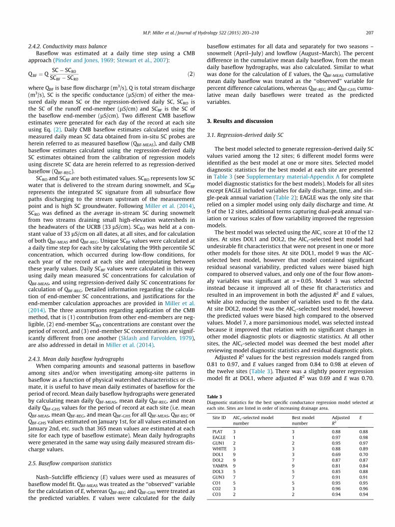
Table 3Diagnostic statistics for the best specific conductance regression model selected ateach site. Sites are listed in order of increasing drainage area.

Site ID AICc-selected modelnumber

Best modelnumber

AdjustedR2

E

PLAT 3 3 0.88 0.88EAGLE 1 1 0.97 0.98GUN1 2 2 0.95 0.97WHITE 3 3 0.88 0.89DOL1 9 3 0.69 0.70DOL2 9 7 0.87 0.87YAMPA 9 9 0.81 0.84DOL3 5 5 0.85 0.88GUN3 7 7 0.91 0.91CO1 5 5 0.95 0.95CO2 3 3 0.96 0.96CO3 2 2 0.94 0.94

M.P. Miller et al. / Journal of Hydrology 522 (2015) 203–210 207

2.4.2. Conductivity mass balanceBaseflow was estimated at a daily time step using a CMB

approach (Pinder and Jones, 1969; Stewart et al., 2007):

Q BF ¼ QSC� SCRO

SCBF � SCROð2Þ

where QBF is base flow discharge (m3/s), Q is total stream discharge(m3/s), SC is the specific conductance (lS/cm) of either the mea-sured daily mean SC or the regression-derived daily SC, SCRO isthe SC of the runoff end-member (lS/cm) and SCBF is the SC ofthe baseflow end-member (lS/cm). Two different CMB baseflowestimates were generated for each day of the record at each siteusing Eq. (2). Daily CMB baseflow estimates calculated using themeasured daily mean SC data obtained from in-situ SC probes areherein referred to as measured baseflow (QBF-MEAS), and daily CMBbaseflow estimates calculated using the regression-derived dailySC estimates obtained from the calibration of regression modelsusing discrete SC data are herein referred to as regression-derivedbaseflow (QBF-REG).

SCRO and SCBF are both estimated values. SCRO represents low SCwater that is delivered to the stream during snowmelt, and SCBF

represents the integrated SC signature from all subsurface flowpaths discharging to the stream upstream of the measurementpoint and is high SC groundwater. Following Miller et al. (2014),SCRO was defined as the average in-stream SC during snowmeltfrom two streams draining small high-elevation watersheds inthe headwaters of the UCRB (33 lS/cm). SCRO was held at a con-stant value of 33 lS/cm on all dates, at all sites, and for calculationof both QBF-MEAS and QBF-REG. Unique SCBF values were calculated ata daily time step for each site by calculating the 99th percentile SCconcentration, which occurred during low-flow conditions, foreach year of the record at each site and interpolating betweenthese yearly values. Daily SCBF values were calculated in this wayusing daily mean measured SC concentrations for calculation ofQBF-MEAS, and using regression-derived daily SC concentrations forcalculation of QBF-REG. Detailed information regarding the calcula-tion of end-member SC concentrations, and justifications for theend-member calculation approaches are provided in Miller et al.(2014). The three assumptions regarding application of the CMBmethod, that is (1) contribution from other end-members are neg-ligible, (2) end-member SCRO concentrations are constant over theperiod of record, and (3) end-member SC concentrations are signif-icantly different from one another (Sklash and Farvolden, 1979),are also addressed in detail in Miller et al. (2014).

2.4.3. Mean daily baseflow hydrographsWhen comparing amounts and seasonal patterns in baseflow

among sites and/or when investigating among-site patterns inbaseflow as a function of physical watershed characteristics or cli-mate, it is useful to have mean daily estimates of baseflow for theperiod of record. Mean daily baseflow hydrographs were generatedby calculating mean daily QBF-MEAS, mean daily QBF-REG, and meandaily QBF-GHS values for the period of record at each site (i.e. meanQBF-MEAS, mean QBF-REG, and mean QBF-GHS for all QBF-MEAS, QBF-REG orQBF-GHS values estimated on January 1st, for all values estimated onJanuary 2nd, etc. such that 365 mean values are estimated at eachsite for each type of baseflow estimate). Mean daily hydrographswere generated in the same way using daily measured stream dis-charge values.

2.5. Baseflow comparison statistics

Nash–Sutcliffe efficiency (E) values were used as measures ofbaseflow model fit. QBF-MEAS was treated as the ‘‘observed’’ variablefor the calculation of E, whereas QBF-REG and QBF-GHS were treated asthe predicted variables. E values were calculated for the daily

baseflow estimates for all data and separately for two seasons –snowmelt (April–July) and lowflow (August–March). The percentdifference in the cumulative mean daily baseflow, from the meandaily baseflow hydrographs, was also calculated. Similar to whatwas done for the calculation of E values, the QBF-MEAS cumulativemean daily baseflow was treated as the ‘‘observed’’ variable forpercent difference calculations, whereas QBF-REG and QBF-GHS cumu-lative mean daily baseflows were treated as the predictedvariables.

3. Results and discussion

3.1. Regression-derived daily SC

The best model selected to generate regression-derived daily SCvalues varied among the 12 sites; 6 different model forms wereidentified as the best model at one or more sites. Selected modeldiagnostic statistics for the best model at each site are presentedin Table 3 (see Supplementary material-Appendix A for completemodel diagnostic statistics for the best models). Models for all sitesexcept EAGLE included variables for daily discharge, time, and sin-gle-peak annual variation (Table 2); EAGLE was the only site thatrelied on a simpler model using only daily discharge and time. At9 of the 12 sites, additional terms capturing dual-peak annual var-iation or various scales of flow variability improved the regressionmodels.

The best model was selected using the AICc score at 10 of the 12sites. At sites DOL1 and DOL2, the AICc-selected best model hadundesirable fit characteristics that were not present in one or moreother models for those sites. At site DOL1, model 9 was the AIC-selected best model, however that model contained significantresidual seasonal variability, predicted values were biased highcompared to observed values, and only one of the four flow anom-aly variables was significant at a = 0.05. Model 3 was selectedinstead because it improved all of these fit characteristics andresulted in an improvement in both the adjusted R2 and E values,while also reducing the number of variables used to fit the data.At site DOL2, model 9 was the AICc-selected best model, howeverthe predicted values were biased high compared to the observedvalues. Model 7, a more parsimonious model, was selected insteadbecause it improved that relation with no significant changes inother model diagnostic plots or diagnostic statistics. At all othersites, the AICc-selected model was deemed the best model afterreviewing model diagnostic statistics and residual diagnostic plots.

Adjusted R2 values for the best regression models ranged from0.81 to 0.97, and E values ranged from 0.84 to 0.98 at eleven ofthe twelve sites (Table 3). There was a slightly poorer regressionmodel fit at DOL1, where adjusted R2 was 0.69 and E was 0.70.

208 M.P. Miller et al. / Journal of Hydrology 522 (2015) 203–210

These regression diagnostic statistics indicate that there wasgenerally good correspondence between the measured discreteSC concentrations and the regression-derived SC concentrations.Further, diagnostic regression plots of residuals showed uniformscatter as a function of fitted values, discharge, and time (seeSupplementary material-Appendix B for plots of model residualsvs fitted values and fitted vs observed values for the best modelsselected at each site).

Fig. 3. Daily discharge, CMB measured baseflow (solid black line), CMB regression-derived baseflow (dashed red line), and GHS baseflow (dashed black line) for a wetyear (water year 2011) and a dry year (water year 2012) at (a) CO1 and (b) DOL1.Note that the scales on the y-axes are variable among sites. (For interpretation ofthe references to color in this figure legend, the reader is referred to the web versionof this article.)

3.2. Comparison of baseflow estimates

Daily QBF-REG estimates were nearly identical to daily QBF-MEAS

estimates with the exception of three sites. Specifically, with theexception of the three Dolores River Sites (DOL1, DOL2, andDOL3), E values comparing QBF-REG to QBF-MEAS were between 0.95and 0.99 (Table 4); indicating a near perfect fit between theQBF-REG and QBF-MEAS estimates. Seasonally, there was little differ-ence between QBF-REG and QBF-MEAS estimates during snowmeltand during low-flow conditions at the non-Dolores River sites,with snowmelt and low-flow E values ranging from 0.96–0.99and 0.85–0.98, respectively. E values comparing QBF-REG andQBF-MEAS estimates at DOL2 and DOL3 were 0.86 and 0.87,respectively; again indicating an excellent fit. There was a worsefit at DOL1, with E = 0.45. Taken together with the regressionmodel diagnostic statistics (Table 3), indicating relatively poormodel fit at DOL1, this result suggests that the moderately poorfit between QBF-REG and QBF-MEAS at this site may be due, at leastin part, to the relatively poor fit obtained by the regression model.

In contrast to the excellent fit between QBF-REG and QBF-MEAS,QBF-GHS deviated from QBF-MEAS at all sites. E values comparingQBF-GHS to QBF-MEAS ranged from �120 to 0.29 (Table 4), with Evalues being <0 at 9 of the 12 sites, indicating that the mean ofQBF-MEAS is a better predictor of baseflow than the QBF-GHS

estimates. QBF-GHS estimates were more similar to QBF-MEAS duringlow-flow conditions than during snowmelt at all sites with theexception of CO1 (i.e. greater E values during low-flow; Table 4).Fig. 3 shows an example of daily baseflow estimates obtained usingthe three approaches during a wet year (water year 2011) and adry year (water year 2012) at a site where there was a good fitbetween QBF-REG and QBF-MEAS estimates (CO1) and a site with arelatively poor fit between QBF-REG and QBF-MEAS estimates (DOL1).At both sites the greatest deviation between QBF-MEAS and QBF-REG

or QBF-GHS occurred during the snowmelt time period.Fig. 4 shows the mean daily baseflow hydrographs for QBF-MEAS,

QBF-REG, and QBF-GHS, expressed as cumulative baseflow volumes. Asobserved for the period of record baseflow estimates, the meandaily cumulative QBF-REG were more similar to the mean dailycumulative QBF-MEAS than were QBF-GHS at all sites. The same

Table 4Nash–Sutcliffe Efficiency (E) values comparing daily CMB measured baseflow (treated as ‘‘baseflow (QBF-GHS) for the period of record at each site. E values were calculated using allperiod only. Also shown are the N-parameter values used for GHS. Sites are listed in orde

Site ID QBF-REG

All times Low-flow Snowmelt

PLAT 0.98 0.96 0.98EAGLE 0.99 0.92 0.98GUN1 0.99 0.98 0.99WHITE 0.99 0.94 0.99DOL1 0.45 0.47 0.34DOL2 0.86 0.83 0.88YAMPA 0.99 0.97 0.98DOL3 0.87 0.81 0.85GUN3 0.98 0.96 0.98CO1 0.98 0.93 0.98CO2 0.98 0.95 0.98CO3 0.95 0.85 0.96

pattern was observed for the ratio of cumulative baseflow tocumulative streamflow (hereafter, BFI), with BFIMEAS values beingmore similar to BFIREG values than BFIGHS at all sites (Table 5).The greatest deviation between mean daily QBF-MEAS and meandaily QBF-REG was at DOL1, where the absolute value of the percentdifference between the cumulative QBF-MEAS and QBF-REG was 51%,followed by DOL3 and DOL2, where the percent differences were18% and 16%, respectively (Table 5). The percent differencebetween the cumulative QBF-MEAS and QBF-REG was 64% for allnon-Dolores River sites. As described in Miller et al. (2014), theDolores River runs through the Paradox Valley, where the Bureauof Reclamation has been intercepting and removing high conduc-tivity groundwater before it discharges to the river for almosttwo decades (Chafin, 2003). This management action has likelyresulted in short-time scale variations in baseflow discharge that

observed’’ value) with daily CMB regression-derived baseflow (QBF-REG) and daily GHSdata, data during the low-flow time period only, and data during the snowmelt timer of increasing drainage area.

QBF-GHS N-parameter

All times Low-flow Snowmelt

0.29 0.57 0.14 13�0.11 �0.46 �0.93 18�10 0.12 �16 60.07 0.39 �0.42 15�5.9 0.21 �9.0 6�120 �2.9 �200 60.20 0.49 �0.33 17�20 �0.05 �43 6�0.98 �0.18 �1.6 11�0.19 �0.51 �0.47 15�0.63 0.45 �1.27 13�0.86 �0.18 �1.57 17

Fig. 4. Cumulative mean daily baseflow for CMB measured baseflow (solid black line), CMB regression-derived baseflow (dashed red line), and GHS baseflow (dashed blackline). Mean daily stream hydrographs are also shown (solid grey line). Sites are listed in order of increasing drainage area from left to right and top to bottom. Note that thescales on the y-axes are variable among sites. (For interpretation of the references to color in this figure legend, the reader is referred to the web version of this article.)

Table 5Cumulative mean daily baseflow for CMB measured baseflow (QBF-MEAS), CMB regression-derived baseflow (QBF-REG), and GHS baseflow (QBF-GHS). The absolute value of thepercent difference between the cumulative mean daily QBF-MEAS (treated as ‘‘observed’’ value) and QBF-REG and QBF-GHS, as well as the BFI values obtained using the CMB measuredbaseflow (MEAS), CMB regression-derived (REG), and GHS hydrograph separation approaches are also shown. Sites are listed in order of increasing drainage area.

Site ID Cumulative baseflow (�107 m3) Percent difference BFIa

QBF-MEAS QBF-REG QBF-GHS QBF-REG (%) QBF-GHS (%) MEAS REG GHS

PLAT 9.50 9.78 7.98 3.0 16 0.54 0.56 0.45EAGLE 11.6 11.9 10.1 2.7 13 0.24 0.24 0.20GUN1 14.1 13.6 24.0 4.0 70 0.29 0.28 0.53WHITE 34.9 36.2 29.5 3.9 16 0.57 0.59 0.47DOL1 6.58 9.96 14.2 51 116 0.24 0.36 0.53DOL2 3.14 3.64 14.8 16 370 0.11 0.12 0.54YAMPA 43.6 42.6 31.8 2.4 27 0.31 0.30 0.22DOL3 12.1 14.2 27.0 18 120 0.28 0.32 0.65GUN3 125 127 166 1.1 33 0.52 0.53 0.74CO1 168 167 196 0.5 17 0.47 0.46 0.54CO2 324 334 368 3.1 14 0.52 0.54 0.61CO3 294 297 311 1.2 5.9 0.47 0.47 0.50

a BFI values calculated as the ratio of the sum of the cumulative baseflow for each hydrograph separation approach (MEAS, REG, or GHS) to the sum of the cumulativestreamflow.

M.P. Miller et al. / Journal of Hydrology 522 (2015) 203–210 209

are difficult to account for with intermittent discrete SC samples;thereby contributing to a relatively large percent differencebetween the cumulative QBF-MEAS and QBF-REG baseflow volumes.While the Dolores River is directly impacted by the interceptionand removal of groundwater, all of the study sites are regulatedto some degree. Taken together, these results suggest that theregression-derived baseflow estimation approach is applicable inregulated streams and rivers, but that caution is warranted whenapplying the approach at sites directly impacted by anthropogenicactivities that alter the natural discharge and/or chemical compo-sition of streams over short time scales.

Cumulative QBF-GHS estimates deviated from the QBF-MEAS esti-mates to a greater extent than did QBF-REG at all sites. As observedfor the example daily data (Fig. 3), the greatest deviation betweenmean daily cumulative QBF-MEAS and QBF-GHS occurred during snow-melt, when the slopes of the mean daily cumulative QBF-GHS base-flow curves deviated most from those of the QBF-MEAS curves(Fig. 4). Cumulative QBF-GHS and BFIGHS values were greater thanQBF-MEAS and BFIMEAS, respectively at 8 of the 12 sites. This findingis consistent with that of Kronholm and Capel (2014), who reportedthat GHS estimates of baseflow were greater than CMB estimates of

baseflow in a stream draining an irrigated watershed in Washing-ton that has a single extended (�5 months) high flow season,similar to that of a snowmelt-dominated hydrograph. CumulativeQBF-GHS deviated most from QBF-MEAS at the Dolores River sites(116–370% difference) and at GUN1 (70% difference, Table 5),where QBF-GHS and BFIGHS were greater than QBF-MEAS and BFIMEAS,respectively. The breakpoint analysis identified N-parameter valuesof 6 as the optimal values at these four sites (Table 4). The absolutevalue of the percent difference between the cumulative QBF-MEAS

and QBF-GHS values at the other sites ranged from 5.9% to 33%(Table 5), where the N-parameter values were between 11 and18. These results suggest that larger N-parameter values (>10 days)are more appropriate than shorter values (<10 days) for estimatingQBF-GHS in snowmelt-dominated systems. This finding is not sur-prising given the extended high flow periods (e.g. 30–90 day snow-melt periods) at the study sites. Taken together these resultssuggest that the breakpoint analysis and subsequent estimationof QBF-GHS using the Wahl and Wahl (1988, 1995) approach maynot be appropriate for use in snowmelt dominated systems, andfuture investigations of if/how the parameters associated with thisGHS approach can be calibrated to better match QBF-MEAS estimates

210 M.P. Miller et al. / Journal of Hydrology 522 (2015) 203–210

is warranted. Comparison of CMB baseflow estimates with esti-mates obtained from other GHS approaches may identify GHSapproaches that are more appropriate for estimating baseflow insnowmelt-dominated streams and rivers.

4. Conclusions

The results of this study demonstrate that baseflow dischargecan be estimated at a daily time step for the period of record ofstream discharge data using discrete SC data and daily stream dis-charge data. These daily baseflow estimates are obtained throughthe development of regression models that relate discrete SC con-centrations to discharge and time, and the application of the CMBhydrograph separation method (a step-by-step summary of howthe approach can be applied is provided in Supplementarymaterial-Appendix C). There was an excellent fit between theregression-derived baseflow estimates and baseflow estimatescalculated from measured high frequency SC data at those siteswhere the regression models were able to accurately model SC.Moreover, regression-derived baseflow estimates were more simi-lar to baseflow estimates obtained from measured high frequencySC data than were estimates obtained using a commonly appliedGHS approach. Among-site comparisons of baseflow estimates sug-gests that GHS N-parameter values of >10 days provide baseflowestimates that are more similar to high frequency SC-derived esti-mates than do shorter N-parameter values (<10 days), but that theGHS approach applied in this study may not be appropriate forsnowmelt-dominated systems without further calibration of modelparameters. Discrepancies between baseflow estimates obtainedusing measured high frequency SC data and those obtained usingthe regression approach at sites on a heavily managed river suggestthat the regression approach should be used with caution at sitesthat are known to experience short time-scale variations in base-flow discharge. These results provide a new approach for estimationof baseflow that can be applied at large numbers of streams and riv-ers. In turn, baseflow estimates at large numbers of sites can be usedto identify watershed or climatic characteristics that influence base-flow discharge to streams and rivers across large spatial scales.

Acknowledgements

We thank R. Hirsch for helpful comments on the developmentof the baseflow estimation approach. C. Corradini, C. Shope, andthree anonymous reviewers provided valuable comments on anearlier version of this manuscript. This study was funded by theU.S. Geological Survey WaterSMART and National Water QualityAssessment Programs.

Appendix A. Supplementary material

Supplementary data associated with this article can be found, inthe online version, at http://dx.doi.org/10.1016/j.jhydrol.2014.12.039.

References

Akaike, H., 1973. Information theory and an extension of the maximum likelihoodprinciple. In: 2nd International Symposium on Information Theory. Tsahkadsor,Armenia, Akadémiai Kiadó, pp. 267–281.

Akaike, H., 1974. A new look at the statistical model identification. IEEE Trans.Autom. Control AC-19 (6), 716–723.

Arnold, J.G., Allen, P.M., 1999. Automated methods for estimating baseflow andground water recharge from streamflow records. J. Am. Water Resour. Assoc. 35,411–424.

Barnes, B.S., 1939. The structure of base flow recession curves. Trans. Am. Geophys.Union 20, 721–725.

Boussinesq, J., 1877. Essai sur la theorie des eaux courantes. Mem. Acad. Sci. Inst.France 23, 252–260.

Chafin, D.T., 2003. Effect of the paradox valley unit on the dissolved-solids load ofthe dolores river near bedrock, Colorado, 1988–2001. U.S. Geol. Surv. Water Res.Invest. Rep., 2002–4275.

Covino, T.P., McGlynn, B.L., 2007. Stream gains and losses across a mountain-to-valley transition: impacts on watershed hydrology and stream water chemistry.Water Resour. Res. 43, W10431.

Ferguson, R.I., 1986. River loads underestimated by rating curves. Water Resour.Res. 22, 74–76.

Gardner, W.P., Susong, D.D., Solomon, D.K., Heasler, H., 2010. Snowmelt hydrographinterpretation: revealing watershed scale hydrologic characteristics of theYellowstone volcanic plateau. J. Hydrol. 383, 209–222.

Genereux, D.P., Jordan, M.T., Carbonell, D., 2005. A apired-watershed budget studyto quantify interbasin groundwater flow in a lowland rain forest. Costa Rica.Water Resour. Res. 41, W04011. http://dx.doi.org/10.1029/2004WR003635.

Guo, Y., Markus, M., Demissie, M., 2002. Uncertainty of nitrate-N load computationsfor agricultural watersheds. Water Resour. Res. 38, 1185. http://dx.doi.org/10.1029/2001WR001149.

Halford, K.J., Mayer, G.S., 2000. Problems associated with estimating ground waterdischarge and recharge from stream-discharge records. Groundwater 38, 331–342.

Hall, F.R., 1968. Base flow recession, a review. Water Resour. Res. 4, 973–983.Hill, R.A., Hawkins, C.P., Carlisle, D.M., 2013. Predicting thermal reference conditions

for USA streams and rivers. Freshwater Sci. 32, 39–55.Hurvich, C.M., Tsai, C.L., 1989. Regression and time series model selection in small

samples. Biometrika 76, 297–307.Institute of Hydrology, 1980a, Low flow studies: Wallingford, Oxon, United

Kingdom, Report No. I, p. 41.Institute of Hydrology, 1980b, Low flow studies: Wallingford, Oxon, United

Kingdom, Report No. 3, pp. 12–19.Kronholm, S., Capel, C., 2014. A comparison of continuous specific conductance-

based end-member mixing analysis and a graphical method for baseflowseparation of four streams in hydrologically challenging agriculturalwatersheds. Hydrol. Process. http://dx.doi.org/10.1002/hyp.10378.

Li, Q., Zing, Z., Danielescu, S., Li, S., Jiang, Y., Meng, F.-R., 2014. Data requirements forusing combined conductivity mass balance and recursive digital filter methodto estimate groundwater recharge in a small watershed New Brunswick. CanadaJ. Hydrol. 511, 658–664.

Lott, D.A., Stewart, M.T., 2013. A power function method for estimating base flow.Groundwater 51, 442–451.

Miller, M.P., Susong, D.D., Shope, C.L., Heilweil, V.H., Stolp, B.J., 2014. Continuousestimation of baseflow in snowmelt-dominated streams and rivers in the UpperColorado River Basin: a chemical hydrograph separation approach. WaterResour. Res. 50, 6986–6999. http://dx.doi.org/10.1002/2013WR014939.

Muggeo, V.M.R., 2008. Segmented: an R package to fit regression models withbroken-line relationships. R News 8 (1), 20–25.

Muggeo, V.M.R., Adelfio, G., 2011. Efficient change point detection in genomicsequences of continuous measurements. Bioinformatics 27, 161–166.

Nash, J.E., Sutcliffe, J.V., 1970. River flow forecasting through conceptual models.Part 1: A discussion of principles. J. Hydrol. 10, 282–290.

Nathan, R.J., McMahon, T.A., 1990. Evaluation of automated techniques for base flowand recession analysis. Water Resour. Res. 26, 1465–1473.

Pellerin, B.A., Wollheim, W.M., Fend, X., Vörösmarty, C.J., 2007. The application ofelectrical conductivity as a tracer for hydrograph separation in urbancatchments. Hydrol. Process. 22, 1810–1818.

Pinder, G.F., Jones, J.F., 1969. Determination of the ground-water component of peakdischarge from the chemistry of total runoff. Water Resour. Res. 5, 438–445.

Preston, S.D., Bierman, V.J., Silliman, S.E., 1989. An evaluation of methods for theestimation of tributary mass loads. Water Resour. Res. 25, 1379–1389.

R Development Team, 2014. The R Project for Statistical Computing (accessed06.03.2014). http://r-project.org.

Ryberg, K.R., Vecchia, A.V., 2012. waterData – an R package for retrieval, analysis,and anomaly calculation of daily hydrologic time series data, version 1.0: U.S.Geol. Surv. Open-File Report 2012-1168.

Ryberg, K.R., Vecchia, A.V., Martin, J.D., Gilliom, R.J., 2010. Trends in pesticideconcentrations in urban streams in the United States, 1992-2008: U.S. Geol.Surv. Scientific Investigations Report 2010-5139.

Sklash, M.G., Farvolden, R.N., 1979. The role of groundwater in storm runoff. J.Hydrol. 43, 45–65.

Stewart, M., Cimino, J., Ross, M., 2007. Calibration of base flow separation methodswith streamflow conductivity. Groundwater 45, 17–27.

Tesoriero, A.J., Duff, J.H., Saad, D.A., Spahr, N.E., Wolock, D.M., 2013. Vulnerability ofstreams to legacy nitrate sources. Environ. Sci. Technol. 47, 3623–3629.

Vecchia, A.V., Martin, J.D., Gilliom, R.J., 2008. Modeling variability and trends inpesticide concentrations in streams. J. Am. Water Resour. Assoc. 44, 1308–1324.

Wahl, K.L., Wahl, T.L., 1988. Effects of regional ground water declines onstreamflows in the Oklahoma Panhandle. In: Proceedings of Symposium onWater-Use Data for Water Resource Management. Tucson, Arizona, Am. WaterResour. As., pp. 239–249.

Wahl, K.L., Wahl, T.L., 1995. Determining the flow of Comal Springs at NewBraunfels, Texas. Texas Water ’95, American Society of Civil Engineers, August16–17, 1995. San Antonio, Texas, pp. 77–86.

Wolock, D.M., 2003. Base-flow index grid for the conterminous United States. U.S.Geol. Surv. Open File Report 03-263.

Zhang, R., Li, Q., Chow, T.L., Li, S., Danielescu, S., 2013. Baseflow separation in a smallwatershed in New Brunswick, Canada, using a recursive digital filter calibratedwith the conductivity mass balance method. Hydrol. Process. 27, 259–2665.