ompared the P 1 closure [10] . However, this comes at the expense
f significantly increased computational costs. Moreover, higher-
rder approximations ( N ≥ 3), result in further increases in compu-
ational effort, whereas the accuracy improvements with increasing
are somewhat more modest [32,33] . For these reasons, it is felt
hat the P 3 approximation provides a reasonable balance between
ccuracy and computational costs.
.4. M N maximum-entropy moment closures
For a given wave number, η, or frequency, the radiative inten-
ity distribution, I η , in the maximum-entropy moment closures is
pproximated by a distribution that maximizes the radiatve en-
ropy, H R ( I η), defined by
R (I η) = 〈 h R 〉 =
∫ 4 π
h R (I η)d�, (9)
nd has a known finite set of moments E (n ) η , n = 0 , . . . , N, where N
s the order of the highest moment in the closed system of mo-
ent equations. In Eq. (9) , h R is the radiative entropy density,
hich corresponds to the entropy for Bose-Einstein statistics in
his case and is given by
R (I η) =
2 kη2
c [(n + 1) ln (n + 1) − n ln (n )] , n =
I η
2 hcη3 , (10)
here n is the occupation number, h and k are the Planck and
oltzmann constants, respectively. The problem of finding a dis-
ribution, I η , that maximizes the radiative entropy given by Eqs.
9) and (10) and subject to the constraints that a finite set of its
ngular moments, E (n ) η , n = 0 , . . . , N, are specified and known can
e reformulated as an optimization problem of the form
η = ∇} �§ I ηH R
(I η)
.t. 〈 � s (n ) I η〉 = E (n ) η , n = 0 , . . . , N.
(11)
he Lagrangian of this optimization problem is
(I η, α) = H R (I η) − αT ( 〈 m
¯( � s ) I η〉 − E η) , (12)
here E η is a vector containing all the independent entries of E (n ) η ,
= 0 , . . . , N, m ( � s ) is a vector containing all the independent en-
ries of � s (n ) , n = 0 , . . . , N, and α is the vector of Lagrange multi-
liers associated with the moment constraints. The entropy max-
mizing distribution, which satisfies ∂ L (I η, α) /∂ I η = 0 , then takes
he form [12]
η(α, m ) = 2 hcη3
[exp
(c 2 hη
k αT m ( � s )
)− 1
]−1
. (13)
n the case of radiation transport in gray media, the distribution
unction Eq. (13) can be integrated over the full spectrum of fre-
uencies ( η ∈ [0, ∞ ]), yielding
(α, m ) =
σste f [αT m ( � s )
]−4 , (14)
π
J.A.R. Sarr and C.P.T. Groth / Journal of Quantitative Spectroscopy & Radiative Transfer 255 (2020) 107238 5
w
p
α
a
M
g
t
b
m
a
w
f
L
O
fl
H
m
r
t
t
p
i
t
o
f
s
3
m
b
t
o
h
t
s
i
t
t
t
w
e
i
I
w
c
χ
a
��I
d
d
n
g
s
t
m
g
o
b
n
h
3
m
o
t
s
t
m
m
d
f
l
f
p
f
s
b
a
t
m
a
M
t
i
i
r
t
m
a
(
t
m
t
r
m
t
a
o
s
d
c
o
m
i
p
r
s
p
p
l
t
o
T
p
t
t
d
v
here σste f = 2 π5 k 4 / 15 c 2 h 3 is the Stephan Boltzmann constant.
In Eq. (14) , the radiative intensity distribution is not given ex-
licitly but is rather expressed in terms of the Lagrange multipliers,
, which have to be determined from the set of nonlinear coupled
lgebraic equations 〈 m ( � s ) I〉 = E. With the exception of the gray
1 model [12] , there exists no analytical expressions for the La-
range multipliers in terms of the angular moments and, as such,
he Lagrange multipliers must therefore be determined numerically
y solving the Lagrangian dual optimization problem for entropy
aximization given by
rg max α{L
∗(α) } , (15)
here L
∗(α) is the Legendre transform of L (I, α) , and has the
orm
∗(α) = −σste f
3 π
⟨[αT m ( � s )
]−3 ⟩− αT E. (16)
nce the Lagrange multipliers have been determined, the closing
ux for the closure can be evaluated using numerical quadrature.
owever, it should be noted that the repeated solution of the opti-
ization problem defined by Eq. (15) whenever an update of the
adiation solutions is required can become very expensive compu-
ationally, particularly as the number of moments increases as is
he case for the higher-order maximum entropy closures in multi-
le space dimensions. For this reason, interpolative-based approx-
mations are proposed in what follows for the closing fluxes of
he gray M 2 closure, which are based on pre-computed solutions
f the optimization problem associated with entropy maximization
or sets of angular moments up to second-order spanning the as-
ociated realizable space.
.5. First-order M 1 maximum-entropy moment closure
The first member of the maximum-entropy hierarchy for gray
edia is the first-order M 1 closure. Unlike other high-order mem-
ers of this hierarchy, analytical expressions for the Lagrange mul-
ipliers in terms of the known set of moments exist in the case
f a gray medium for the M 1 closure. Similar, to the P 1 spherical
armonic approximation, the M 1 model achieves closure by using
he entropy maximizing distribution of Eq. (14) and expressing the
econd-order moment dyad in terms of the lower-order moments,
.e., I (2) = I (2) (I (0) , I (1) ) . Another feature of the first-order closure is
hat the anisotropy in the underlying radiative distribution lies in
he direction of the first-order moment vector or flux, I (1) . This in
urn implies that the radiative intensity distribution is symmetric
ith respect to the direction of N
(1) = I (1) /I (0) . Using this prop-
rty, Levermore [34] previously derived an expression for the clos-
ng flux of the M 1 closure which takes the form
(2) = N
(2) I (0) , N
(2) =
1 − χ
2
� � I +
3 χ − 1
2
� n � �
n , (17)
here χ is the well-known Eddington factor and, for the gray M 1
losure, is given by
=
3 + 4 ‖ N
(1) ‖
2
5 + 2 ξ, ξ =
√
4 − 3 ‖ N
(1) ‖
2 , (18)
nd where N
(n ) = I (n ) /I (0) are the n th -order normalized moments,
is the identity dyad, and
� n = N
(1) / ‖ N
(1) ‖ is the unit vector in the
irection of the first-order moment.
In spite of its ability to capture a wider range of optical con-
itions than the P 1 model, the M 1 closure is known to produce
onphysical discontinuities in the radiative energy density and also
enerally provide inaccurate predictions of radiative quantities for
ituations in which beams of photons travelling in opposite direc-
ions cross [14] . In fact, when the zeroth- and first-order angular
oments are the only available information for reconstructing a
iven distribution, the only possible form for the latter in the case
f crossing beams with zero net flux is that of an isotropic distri-
ution, even though the underlying angular distributions are highly
on-isotropic. This issue can however be remedied by considering
igh-order members of the maximum-entropy hierarchy.
.6. Second-order M 2 maximum-entropy moment closure
The next member of the maximum-entropy hierarchy for gray
edia is the second-order M 2 closure and is the primary focus
f the present study. In a procedure similar to that described for
he M 1 closure, transport equations for known moments up to
econd-order are closed by assuming an entropy maximizing dis-
ribution and subsequently expressing the third-order closing mo-
ents (second-order moment fluxes), I (3) , in terms of the known
oments, i.e., I (3) = I (3) (I (0) , I (1) , I (2) ) or, in the case of gray me-
ia, N
(3) = N
(3) (N
(1) , N
(2) ) ). Unfortunately, unlike the M 1 closure
or a gray medium, it is not possible to obtain a closed-form ana-
ytical expression for the closing moment flux of the M 2 closure (in
act, a closed-form analytical expression for the closing flux is only
ossible for the M 1 model in the case of gray media) and there-
ore, in the simulations of radiative transport, repeated numerical
olution of the optimization problem defined by Eq. (15) would
e necessary, making the application of the closure computation-
lly expensive.
To circumvent the need for the costly solutions of the optimiza-
ion problem to determine the Lagrange multipliers defining the
aximum entropy distribution, an alternative interpolative-based
pproach for accurately approximating the closing flux for the gray
2 closure is proposed herein which attempts to retain many of
he desirable properties of the original model (e.g., moment real-
zability and hyperbolicity of the moment equations) while result-
ng in substantially reduced computational costs compared to the
epeated solution of the optimization problem. The proposed in-
erpolant is formulated to closely match the form of the M 2 maxi-
um entropy solution within the entire space of physically realiz-
ble moments defined by the angular moments up to second-order
i.e., the space defined by the set of necessary and sufficient condi-
ions such that there exists a non-negative distribution reproducing
oments of the M 2 closure). More specifically, an affine combina-
ion of the known analytical forms of N
(3) on the boundaries of
ealizable space in terms of N
(1) and N
(2) is adopted as an approxi-
ation to the closing relation. The interpolant is then extended to
he interior of realizable space via a fitting procedure such that it
pproximates pre-computed values of N
(3) obtained by solving the
ptimization problem for entropy maximization for moment sets
panning the full range of realizable space. The development and
escription of the proposed interpolative-based second-order M 2
losure are given below in the section to follow.
It should be noted that several authors have recently devel-
ped analytical approximations to the M 2 maximum-entropy mo-
ent closure in multi-dimensional space. Firstly, as noted in the
ntroduction, Pichard et al . [19] proposed an extension of the
reviously-developed approximation to the M 2 closure by Mon-
eal and Frank [18] for one space dimension to multiple dimen-
ions. The multi-dimensional interpolative-based M 2 closure pro-
osed by Pichard et al. [19] was formulated for radiative trans-
ort obeying Boltzmann statistics. More specifically, their interpo-
ation attempts to mimic the maximum entropy solutions only in
he case where the first-order moment, N
(1) , coincides with one
f the eigenvectors of the covariance matrix, (N
(2) − N
(1) (N
(1) ) T ) .
heir approximation of the maximum entropy solutions was com-
rised of several steps. Firstly, an interpolative-based approxima-
ion of the closure relation for the M 2 closure, in the case where
he covariance matrix has at least two identical eigenvalues, was
eveloped. This approximation was obtained by means of con-
ex combinations between the upper and lower boundaries of the
6 J.A.R. Sarr and C.P.T. Groth / Journal of Quantitative Spectroscopy & Radiative Transfer 255 (2020) 107238
f
c
l
i
f
H
4
u
r
g
t
d
T
o
h
i
s
s
F
t
s
t
t
s
t
f
a
d
T
n
d
c
g
s
P
I
b⟨
w
r
M
m
n
w
m
m
d
c
d
d
R
T
i
b
t
realizablity constraints on the highest-order moments, the analyt-
ical expressions of which are available in this particular case. The
approximation was then extended to more general sets of eigen-
values for the covariance matrix, by means of polynomial inter-
polation, which reproduces known analytical expressions for the
closure relations in the case of degenerate eigenvalues, and also
reproduces the approximation corresponding to the case with at
least two identical eigenvalues. The choice of polynomial interpo-
lation, instead of convex combinations, at this stage of the approx-
imation was justified by the fact that, unlike the case with at least
two identical eigenvalues, there exist to date no necessary and suf-
ficient realizability conditions for the third-order moment, N
(3) , in
more general cases. Extension to the full realizability domain for
moments up to order two was then achieved by means of con-
vex combinations within the unit ball described by the realizabil-
ity constraints on the first-order moment. By its construction, the
resulting interpolative-based M 2 closure, was proven to be realiz-
able for sets of moments up to second-order for which the covari-
ance matrix has at least two identical eigenvalues and one of its
eigenvector is co-linear to N
(1) . Moreover, the maximum-entropy
solutions are only well approximated in a portion of the full re-
alizable space for moments up to second-order. Finally, it can be
shown that the description of the closure relations used by Pichard
et al. [19] on some of the boundaries of the realizable domain for
moments up to second-order is problematic, making the applica-
tion to the full range of practical simulations very difficult.
More recently, an extended quadrature method of moments
(EQMOM)-based second-order moment closure was developed by
Li et al. [35] , as an approximation to the M 2 maximum-entropy
closure. In their approach, the base function used in the EQMOM
scheme are β probability density functions. One of the main ad-
vantages of this so-called B 2 model of Li et al. [35] , compared
to the M 2 closure, is the existence of closed-form analytical ex-
pressions for the closure relation. Moreover, the B 2 model pro-
vides a smooth interpolation between the isotropic and the free-
streaming limits. However, the EQMOM-based closure does not re-
ally attempt to mimic closely the properties of the M 2 maximum
entropy closure and the B 2 model in multiple space dimensions
is neither globally realizable nor globally hyperbolic. In fact, Li
et al. [35] have shown that the quadrature-based approximation
to the M 2 closure is only realizable and hyperbolic in a portion of
the realizable space defined by moments up to second-order.
4. Interpolative-based second-order M 2 maximum-entropy
moment closure
In this section, the new interpolative-based approximation of
the second-order maximum entropy, M 2 , closure is formulated for
radiative transfer in multi-dimensional, gray, participating media.
Our proposed interpolant is formulated such that the known ana-
lytical expressions of the closing fluxes on the boundaries of real-
izable space are exactly reproduced. Using a polynomial interpola-
tion procedure, the affine interpolant is then extended to match
identically a range of pre-computed solutions of the optimiza-
tion problem for entropy maximization for sets of moments span-
ning the full realizable space for moments up to second-order, as
well as derivatives of the highest-order moment on the bound-
aries. This fitting of the pre-computed solutions is achieved by the
use of orthogonal or near orthogonal polynomial basis functions
so as to optimize the condition number of the resulting Vander-
monde matrix and consequently facilitate the inversion of the lat-
ter. The nodes for the interpolation procedure are chosen to co-
incide with roots of Chebyshev polynomials, which are known to
provide quasi-optimal approximation to any given function. In the
near vicinity of the boundaries of the realizable moment space, the
numerical solution of the highly nonlinear optimization problem
or entropy maximization becomes increasingly difficult, due to ill-
onditioning of the Hessian matrix. In order to facilitate the so-
ution of the optimization problem in these regions, precondition-
ng of the Hessian matrix is applied as described in Section 4.3 to
ollow, which substantially improves the condition number of the
essian such that its inverse can be computed with good accuracy.
.1. Necessary and sufficient conditions for realizability of moments
p to second-order
As a first step, the necessary and sufficient conditions for
ealizability of moments up to second-order are presented and
iven. A proof of sufficiency is also provided. These conditions and
he proof were previously established for both one- and multi-
imensional radiative heat transfer problems by Kershaw [22] .
hey were also key elements in the construction of the previ-
us second-order closures of Pichard et al. [19] and Li et al. [35] ;
owever, as they are crucial to the development of the proposed
nterpolative-based approximation of the M 2 closure, they are re-
ummarized here. Note that proof of sufficiency given here is a
light variant of Kershaw’s proof and follows that of Monreal and
rank [18,36] for the one-dimensional case, with an extension to
he multi-dimensional case.
Realizability of the predicted angular moments of a given clo-
ure deals with the issue of whether or not a physically realis-
ic (i.e., strictly positive valued or non-negative) angular distribu-
ion of the radiation intensity can be associated with the given
et of moments. If such an angular distribution can be identified,
hen the moment set is deemed to be realizable. The conditions
or moment realizability give rise to a set of constraints or realiz-
bility conditions on the predicted moments which can be used to
efine the extent of possible closure solutions in moment space.
he approach essentially consists of multiplying a presumed non-
egative distribution by a non-negative polynomial test function
efined in terms of the angular variables, from which necessary
onditions for realizability of the moments can be derived. For a
iven set of N angular weights, S (N) = [1 , � s (1) , � s (n ) , . . . ] T , and corre-
ponding moments, I (N) = 〈 S (N) I〉 , one can construct a polynomial,
(N) ( � v ) = a T S (N) , where a T are the coefficients of the polynomial.
t then follows that for any globally positive-valued angular distri-
ution, I , and polynomial, P
(N) , one must have
||P
(N) ( � v ) || 2 I ⟩ = a T ⟨S (N)
[S (N)
]T I ⟩a ≥ 0 , (19)
hich, for an arbitrary polynomial, requires that the real symmet-
ic matrix, M
( N ) , given by
(N) =
⟨S (N)
[S (N)
]T I ⟩, (20)
ust be positive definite. For situations in which this matrix is
egative definite, it follows that the moment set is not consistent
ith any possible positive-valued distribution, I , and, hence, the
oments are not physically realizable. For the M 2 closure and mo-
ents up to second-order for an every-where non-negative angular
istribution of the radiative intensity, the corresponding necessary
onditions on moment realizability, which define the realizability
omain for moments up to second order denoted by R
2 , can be
efined as follows [18,22,36] :
2 = { (I (0) , I (1) , I (2) ) ∈ R
3 × R
3 ×3 , s.t. I (0) ≥ 0 , ‖ N
(1) ‖ ≤ 1 ,
N
(2) − N
(1) (N
(1) ) T ≥ 0 , � n
T N
(2) � n ≤ 1 ∀ ‖
� n ‖ ≤ 1 ,
tr(N
(2) ) = 1 and N
(2) i j
= N
(2) ji
} . (21)
he proof of the existence of a non-negative distribution reproduc-
ng moments in R
2 also provides a proof that conditions R
2 are
oth necessary and sufficient. The former can be demonstrated via
he application of a suitable transformation of R
2 such that the
J.A.R. Sarr and C.P.T. Groth / Journal of Quantitative Spectroscopy & Radiative Transfer 255 (2020) 107238 7
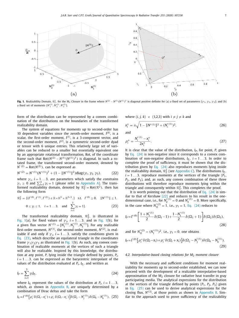
Fig. 1. Realizability Domain, R
2 T , for the M 2 Closure in the frame where N (2) − N (1) (N (1) ) T is diagonal positive definite for (a) a fixed set of parameters { γ 1 , γ 2 , γ 3 }; and (b)
a fixed set of moments { N ’ (1) 1
, N ’ (1) 2
, N ’ (1) 3
} .
f
n
r
1
s
t
o
a
b
f
t
N
N
w
γf
t
R
F
a
fi
i
E
f
b
w
t
i
v
I
w
w
c
I
w
x
a
ρ
I
b
b
c
t
t
i
P
d
t
i
d
i
I
a
I
4
i
p
a
p
a
i
c
i
orm of the distribution can be represented by a convex combi-
ation of the distributions on the boundaries of the transformed
ealizability domain.
The system of equations for moments up to second-order has
0 dependent variables since the zeroth-order moment, I (0) , is a
calar, the first-order moment, I (1) , is a 3-component vector, and
he second-order moment, I (2) , is a symmetric second-order dyad
r tensor with 6 unique entries. This relatively large set of vari-
bles can be reduced to a smaller but essentially equivalent one
y an appropriate rotational transformation, Rot, of the coordinate
rame such that Rot (N
(2) − N
(1) (N
(1) ) T ) is diagonal. In such a ro-
ated frame, the transformed second-order moment, denoted by
’ (2) = Rot (N
(2) ) , can be expressed as
′ (2) = N
′ (1) (N
′ (1) ) T + (1 − ‖ N
′ (1) ‖
2 ) diag (γ1 , γ2 , γ3 ) . (22)
here γ i , i = 1 . . . 3 , are parameters which satisfy the constrains
i ≥ 0 and∑ 3
i =1 γi = 1 (please refer to Appendix A ). The trans-
ormed realizability domain, denoted by R
2 T = Rot (R
2 ) , then has
he following form
2 T = { (I ′ (0) , I ′ (1) , I ′ (2) ) ∈ R ×R
3 × R
3 ×3 , } s.t. I ′ (0) ≥ 0 , ‖ N
′ (1) ‖ ≤ 1 ,
0 ≤ γi ≤ 1 , i = 1 . . . 3 , and
3 ∑
i =1
γi = 1 } . (23)
The transformed realizability domain, R
2 T , is illustrated in
ig. 1 (a), for fixed values of γ i , i = 1 . . . 3 , and in Fig. 1 (b), for
given flux vector N
′ (1) = [ N
′ (1) 1
, N
′ (1) 2
, N
′ (1) 3
] . For any realizable
rst-order moment, N
′ (1) , the second-order moment, N
′ (2) , is real-
zable if and only if γ i , i = 1 . . . 3 , satisfy the conditions given in
q. (23) , which describe an equilateral triangle in the coordinates
rame γ 1 γ 2 γ 3 as illustrated in Fig. 1 (b). As such, any convex com-
ination of realizable moments at the vertices of such a triangle
ill also be realizable. Inspired by this knowledge, the distribu-
ion at any point, P , lying inside the triangle defined by points, P i ,
= 1 . . . 3 , can be expressed as the barycentric interpolant of the
alues of the distribution evaluated at P i , I P i , and written as
P =
3 ∑
i =1
γi I P i , (24)
here I P i represent the values of the distribution at P i , i = 1 . . . 3 ,
hich, as shown in Appendix B , are uniquely determined by a
ombination of Dirac deltas and take the form
P i = I ′ (0) [ρ+
i δ(�i −x +
i ) + ρ−
i δ(�i −x −
i ) ]δ(� j − N
′ (1) j
) δ(�k − N
′ (1) k
) , (25)
here ( i, j, k ) ∈ (1,2,3) with i � = j � = k and
±i
= ±√
1 − ‖ N
′ (1) ‖
2 + (N
′ (1) i
) 2 , (26)
nd
±i
=
N
′ (1) i
− x ∓i
2 x ±i
. (27)
t is clear that the value of the distribution, I P , for point, P , given
y Eq. (24) is non-negative since it corresponds to a convex com-
ination of non-negative distributions, I P i , i = 1 . . . 3 . In order to
omplete the proof of sufficiency, it must be shown that the dis-
ribution given by Eq. (24) also reproduces moments lying inside
he realizability domain, R
2 T (see Appendix C ). The distributions I P i ,
= 1 . . . 3 , reproduce moments at the vertices of the triangle ( P 1 ,
2 , and P 3 ), and, as such, any convex combination of these three
istributions will therefore reproduce moments lying within the
riangle and consequently within R
2 T . This completes the proof.
It is worth pointing out that the distribution of Eq. (24) is sim-
lar to that of Kershaw [22] and reduces to his result in the one-
imensional case, i.e., for N
′ (1) 2
= 0 and N
′ (1) 3
= 0 . More specifically,
n the case where N
′ (2) 11
= 1 , i.e., γ1 = 1 , Eq. (24) reduces to
P = I ′ (0)
[1 + N
′ (1) 1
2
δ(�1 −1) +
1 −N
′ (1) 1
2
δ(�1 + 1)
]δ(�2 ) δ(�3 ) ,
(28)
nd for N
′ (2) 11
= (N
′ (1) 1
) 2 , i.e., γ1 = 0 , one obtains
P = I ′ (0) [ρ+
i δ(�i −x i ) + ρ−
i δ(�i + x i )
]δ(� j − N
′ (1) j
) δ(�k − N
′ (1) k
) .
(29)
.2. Interpolative-based closing relations for M 2 moment closure
With the necessary and sufficient conditions for moment real-
zability for moments up to second-order established, we can now
roceed with the development of a realizable interpolative-based
pproximation of the M 2 closure for radiative heat transfer in gray
articipating media. The analytical expressions for the distribution
t the vertices of the triangle defined by points ( P 1 , P 2 , P 3 ) given
n Eq. (25) can be used to derive analytical expressions for the
losing flux, N
′ (3) , at those points as shown in Appendix B . Sim-
lar to the approach used to prove sufficiency of the realizability
8 J.A.R. Sarr and C.P.T. Groth / Journal of Quantitative Spectroscopy & Radiative Transfer 255 (2020) 107238
Table 1
Exact Analytic Expression of M 2 Closure Relation at the Vertices of the Triangle P 1 , P 2 , P 3 .
Vertex N ′ (3) 111
N ′ (3) 122
N ′ (3) 123
P 1 N ′ (1) 1
[(N ′ (1)
1 ) 2 + (1 − ‖ N ′ (1) ‖ 2 ) ] N ′ (1)
1 (N
′ (1) 2
) 2 N ′ (1) 1
N ′ (1) 2
N ′ (1) 3
P 2 (N ′ (1) 1
) 3 N ′ (1) 1
[(N ′ (1)
2 ) 2 + (1 − ‖ N ′ (1) ‖ 2 ) ] N
′ (1) 1
N ′ (1) 2
N ′ (1) 3
P 3 (N ′ (1) 1
) 3 N ′ (1) 1
(N ′ (1) 2
) 2 N ′ (1) 1
N ′ (1) 2
N ′ (1) 3
e
(
N ,
N ,
N
w
g
m
l
θ
a
γ
p
a
p
c
i
p
t
w
θ
m
o
g
conditions for moments up to order two, the closing flux relations
for the M 2 closure within R
2 T are approximated by affine combina-
tions of the exact analytical expressions at points P i , i = 1 . . . 3 (see
Table 1 ). The interpolant is chosen such that the closures approxi-
mate their corresponding numerical values obtained by solving the
optimization problem for entropy maximization, Eq (15) , for sets of
moments spanning R
2 T
. More specifically, the approximation of the
closing flux in the rotated frame, N
′ (3) , is assumed to take the form
N
′ (3) i jk
=
3 ∑
i =1
f (γi ) N
′ (3) i jk
(P i ) . (30)
where f ( γ i ) are weighting functions satisfying ∑ 3
i =1 f (γi ) = 1 . Once
approximations of the closing moment fluxes in R
2 T
are obtained,
the closing relations for R
2 can then be derived through the in-
verse transformation of R
2 T
→ R
2 as defined by
T : R
2 T → R
2 (I ′ (0) , I ′ (1) , I ′ (2) ) → (I (0) , I (1) , I (2) )
s.t. I ′ (0) = I (0) , I ′ (1) i
= R i j I (1) j
, I ′ (2) i j
= R im
I (2) mn R n j
(31)
where R ij is the rotation matrix such that R T (N
(2) − N
(1) (N
(1) ) T ) R
is diagonal positive definite.
The third-order normalized moment tensor, N
′ (3) , is symmetric
and therefore has just 10 unique entries. Knowledge of just 3 of
these entries, namely N
′ (3) 111
, N
′ (3) 122
and N
′ (3) 123
, is sufficient to obtain
values for the remaining 7 entries which can be related to these 3
entries as follows:
N ’ ( 3 )
222
(N ’ (
1 ) 1
, N ’ ( 1 )
2 , N ’ (
1 ) 3
, γ1 , γ2
)= N ’ (
3 ) 111
(N ’ (
1 ) 2
, −N ’ ( 1 )
1 , N ’ (
1 ) 3
, γ2 , γ1
),
N ’ ( 3 )
333
(N ’ (
1 ) 1
, N ’ ( 1 )
2 , N ’ (
1 ) 3
, γ1 , γ2
)= N ’ (
3 ) 111
(N ’ (
1 ) 3
, N ’ ( 1 )
2 , −N ’ (
1 ) 1
, 1 − γ1 − γ2 , γ2
),
N ’ ( 3 )
112
(N ’ (
1 ) 1
, N ’ ( 1 )
2 , N ’ (
1 ) 3
, γ1 , γ2
)= N ’ (
3 ) 122
(N ’ (
1 ) 2
, −N ’ ( 1 )
1 , N ’ (
1 ) 3
, γ2 , γ1
),
N ’ ( 3 )
113
(N ’ (
1 ) 1
, N ’ ( 1 )
2 , N ’ (
1 ) 3
, γ1 , γ2
)= N ’ (
3 ) 122
(N ’ (
1 ) 3
, N ’ ( 1 )
1 , N ’ (
1 ) 2
, 1 − γ1 − γ2 , γ1
),
N ’ ( 3 )
133
(N ’ (
1 ) 1
, N ’ ( 1 )
2 , N ’ (
1 ) 3
, γ1 , γ2
)= N ’ (
3 ) 122
(N ’ (
1 ) 1
, N ’ ( 1 )
3 , −N ’ (
1 ) 2
, γ1 , 1 − γ1 − γ2
),
N ’ ( 3 )
223
(N ’ (
1 ) 1
, N ’ ( 1 )
2 , N ’ (
1 ) 3
, γ1 , γ2
)= N ’ (
3 ) 122
(N ’ (
1 ) 3
, N ’ ( 1 )
2 , −N ’ (
1 ) 1
, 1 − γ1 − γ2 , γ2
),
N ’ ( 3 )
233
(N ’ (
1 ) 1
, N ’ ( 1 )
2 , N ’ (
1 ) 3
, γ1 , γ2
)= N ’ (
3 ) 122
(N ’ (
1 ) 2
, N ’ ( 1 )
3 , N ’ (
1 ) 1
, γ2 , 1 − γ1 − γ2
).
(32)
The optimization problem for entropy maximization given by
Eq. (15) cannot be solved on directly everywhere on the bound-
aries of the realizability domain R
2 T , denoted as ∂R
2 T , as the cor-
responding entropy maximizing distribution can become singular
due to the fact that propagation of radiation is then only allowed
along specific directions or becomes planar, instead of spanning
the full solid angle. In these situations, the intensity distribution
is either uniquely determined by a Dirac delta distribution or a
combination of Dirac delta distributions, or an entropy maximizing
distribution describing propagation of radiation on the (unit) circle
as discussed in Appendix B . Pre-computed values of N
(3) can then
be obtained by solving the appropriate optimization problem for
entropy maximization in the interior of R
2 T
and in regions of ∂R
2 T
where exact analytical expressions for N
(3) are not available.
Based on the interpolation used to prove sufficiency of the con-
ditions for moment realizability up to second-order and the known
xact analytical form of N ’ (3) 111
, N ’ (3) 122
, N ’ (3) 123
on the boundaries of R
2 T
see Table 1 ), the following approximations are proposed:
’ ( 3 )
111 ( ‖ N ’ ( 1 ) ‖ , θ, φ, γ1 , γ2 ) = N ’ ( 1 )
1
[(N ’ (
1 ) 1
)2
+ f N ’
( 3 ) 111
( 1 − ‖ N ’ ( 1 ) ‖ 2 )]
(33)
’ ( 3 )
122 ( ‖ N ’ ( 1 ) ‖ , θ, φ, γ1 , γ2 ) = N ’ ( 1 )
1
[(N ’ (
1 ) 2
)2
+ f N ’
( 3 ) 122
( 1 − ‖ N ’ ( 1 ) ‖ 2 )]
(34)
’ ( 3 )
123 ( ‖ N ’ ( 1 ) ‖ , θ, φ, γ1 , γ2 ) = f N ’ (
3 ) 123
N ’ ( 1 )
1 N ’ (
1 ) 2
N ’ ( 1 )
3 , (35)
here θ and φ, respectively represent the polar and azimuthal an-
les characterizing the direction of the first-order normalized mo-
ent, N’ (1) , in a spherical coordinate system and are defined as fol-
ows
= arccos
(N ’ (
1 ) 3
‖ N ’ ( 1 ) ‖
), φ = arccos
⎛
⎝
N ’ ( 1 )
1 √ (N ’ (
1 ) 1
)2 +
(N ’ (
1 ) 2
)2
⎞
⎠ ,
(36)
nd f N ’
(3) 111
= f N ’
(3) 111
(‖ N ’ (1) ‖ , θ, φ, γ1 , γ2 ) , f N ’
(3) 122
= f N ’
(3) 122
(‖ N ’ (1) ‖ , θ, φ,
1 , γ2 ) , and f N ’
(3) 123
= f N ’
(3) 123
(‖ N ’ (1) ‖ , θ, φ, γ1 , γ2 ) are polynomial ex-
ressions defined such that the approximations of the closing flux
ccurately reproduce pre-computed solutions of the optimization
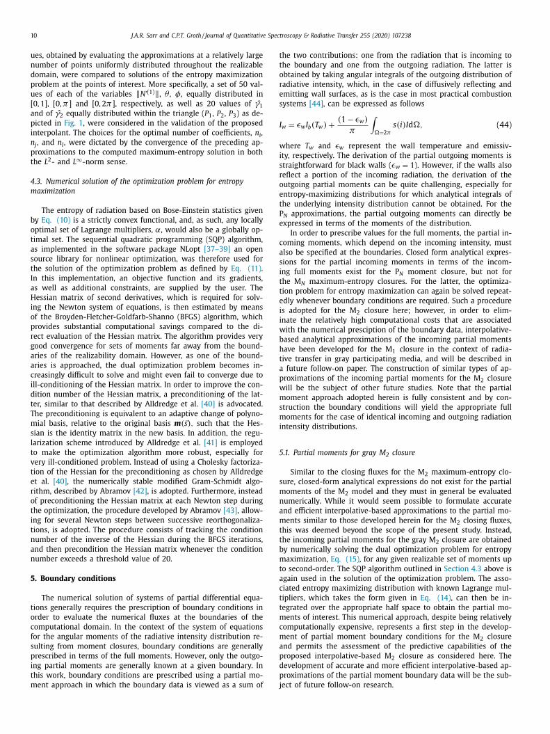
roblem for entropy maximization. For illustration purposes, iso-
ontours of f N ’
(3) 111
, f N ’
(3) 122
, and f N ’
(3) 123
, over the triangle P 1 P 2 P 3 are
llustrated in Figs. 2 (a), (b), and (c), respectively. For accurately ap-
roximating the pre-computed solutions as well as derivatives on
he boundaries of the realizable space, we choose to write f N ’
(3) 111
,
f N ’
(3) 122
, and f N ’
(3) 123
as affine combinations of the form
f N ’ (
3 ) 111
( ‖ N ’ ( 1 ) ‖ , θ, φ, γ1 , γ2 ) = γ1
[ 1 + ( 1 − γ1 ) g N ’ ( 3 )
111
] , (37)
f N ’ (
3 ) 122
( ‖ N ’ ( 1 ) ‖ , θ, φ, γ1 , γ2 ) = γ2
[ 1 + γ1 g N ’ ( 3 )
122
] , (38)
f N ’ (
3 ) 123
( ‖ N ’ ( 1 ) ‖ , θ, φ, γ1 , γ2 ) = 1 + γ1 γ2 γ3 g N ’ ( 3 ) 123
, (39)
here g N ’
(3) 111
= g N ’
(3) 111
(‖ N ’ (1) ‖ , θ, φ, γ1 , γ2 ) , g N ’
(3) 122
= g N ’
(3) 122
(‖ N ’ (1) ‖ ,, φ, γ1 , γ2 ) , and g
N ’ (3) 123
= g N ’
(3) 123
(‖ N ’ (1) ‖ , θ, φ, γ1 , γ2 ) are polyno-
ial expressions which are written as series expansion in terms
f orthogonal basis functions as follows
N ’ ( 3 )
111
=
n i ∑
i =0
n j ∑
j=0
j ∑
k = − j
n l ∑
l=0
n m ∑
m =0
C N ’ (
3 ) 111
ijklm
T 2 i ( ‖ N ’ ( 1 ) ‖ ) Y k j ( θ, φ) T l (
ˆ γ1
)T m
(ˆ γ2
),
(40)
J.A.R. Sarr and C.P.T. Groth / Journal of Quantitative Spectroscopy & Radiative Transfer 255 (2020) 107238 9
Fig. 2. Isocontours of (a) f N ’ 3 111
; (b) f N ’ 3 122
and (c) f N ’ 3 123
over the triangle P 1 P 2 P 3 for N ’ (1) 1
= 0 . 4 , N ’ (1) 2
= 0 . 2 , N ’ (1) 3
= 0 . 15 .
g
g
w
p
γ
a
a
d
k
k
t
a
p
s
t
a
o
f
f
a
m
n
s
d
c
p
N ’ ( 3 )
122
=
n i ∑
i =0
n j ∑
j=0
j ∑
k = − j
n l ∑
l=0
n m ∑
m =0
C N ’ (
3 ) 122
ijklm
T 2 i ( ‖ N ’ ( 1 ) ‖ ) Y k j ( θ, φ) T l (
ˆ γ1
)T m
(ˆ γ2
),
(41)
N ( 3 )
123
=
n i ∑
i =0
n j ∑
j=0
j ∑
k = − j
n l ∑
l=0
n m ∑
m =0
C N ’ (
3 ) 123
ijklm
T 2 i ( ‖ N ’ ( 1 ) ‖ ) Y k j ( θ, φ) T l (
ˆ γ1
)T m
(ˆ γ2
),
(42)
here ˆ γ1 and ˆ γ2 are obtained through a rectangle-triangle map-
ing of the form
1 =
1 + ˆ γ1
2
2 − (1 − ζ )(1 + ˆ γ2 )
2
, γ2 =
1 + ˆ γ2
2
2 − ζ (1 + ˆ γ1 )
2
,
(43)
nd where ζ is a parameter for the mapping. In Eqs. (40) , (41) ,
nd (42) , T n is a Chebyshev polynomial of the first kind of or-
er n , Y k j
is a spherical harmonic function of degree j and order
, and C N ’
(3) 111
ijklm
, C N ’
(3) 122
ijklm
, as well as C N ’
(3) 123
ijklm
, i = 0 , . . . , n i , j = 0 , . . . , n j ,
= − j, . . . , j, l = 0 , . . . , n l , m = 0 , . . . , n m
are coefficients to be de-
ermined such that the proposed approximation of the M 2 closure
ccurately reproduces pre-computed solutions of the optimization
roblem for entropy maximization for sets of moments up to
econd-order spanning the full realizable space. The coefficients of
he interpolant are computed by solving the Vandermonde system
rising from the enforcement of Eqs. (40) , (41) , and (42) at vari-
us nodal points throughout the realizable space. Following a care-
ul analysis of the numerical solutions of the optimization problem
or entropy maximization, the interpolation points for ‖ N’ (1) ‖ , ˆ γ1 ,
nd ˆ γ2 were chosen to coincide with roots of Chebyshev polyno-
ials of order 2 n i , n l , and n m
, respectively, for given values of n i ,
l , and n m
. On the other hand, the interpolation nodes for θ were
elected to correspond to roots of the Legendre polynomials of or-
er n j and a set of 2 n j points uniformly distributed on the unit
ircle are chosen for φ. In order to assess the accuracy of the pro-
osed interpolative-based approximation of the M 2 closure, its val-
10 J.A.R. Sarr and C.P.T. Groth / Journal of Quantitative Spectroscopy & Radiative Transfer 255 (2020) 107238
t
t
o
r
e
s
I
w
i
s
r
o
e
t
P
e
c
a
s
i
t
t
e
i
i
w
b
h
t
a
p
w
m
s
m
i
5
s
m
n
a
m
t
t
b
m
t
a
c
t
t
m
c
m
a
p
d
p
j
ues, obtained by evaluating the approximations at a relatively large
number of points uniformly distributed throughout the realizable
domain, were compared to solutions of the entropy maximization
problem at the points of interest. More specifically, a set of 50 val-
ues of each of the variables ‖ N’ (1) ‖ , θ , φ, equally distributed in
[0, 1], [0, π ] and [0, 2 π ], respectively, as well as 20 values of ˆ γ1
and of ˆ γ2 equally distributed within the triangle ( P 1 , P 2 , P 3 ) as de-
picted in Fig. 1 , were considered in the validation of the proposed
interpolant. The choices for the optimal number of coefficients, n i ,
n j , and n l , were dictated by the convergence of the preceding ap-
proximations to the computed maximum-entropy solution in both
the L 2 - and L ∞ -norm sense.
4.3. Numerical solution of the optimization problem for entropy
maximization
The entropy of radiation based on Bose-Einstein statistics given
by Eq. (10) is a strictly convex functional, and, as such, any locally
optimal set of Lagrange multipliers, α, would also be a globally op-
timal set. The sequential quadratic programming (SQP) algorithm,
as implemented in the software package NLopt [37–39] an open
source library for nonlinear optimization, was therefore used for
the solution of the optimization problem as defined by Eq. (11) .
In this implementation, an objective function and its gradients,
as well as additional constraints, are supplied by the user. The
Hessian matrix of second derivatives, which is required for solv-
ing the Newton system of equations, is then estimated by means
of the Broyden-Fletcher-Goldfarb-Shanno (BFGS) algorithm, which
provides substantial computational savings compared to the di-
rect evaluation of the Hessian matrix. The algorithm provides very
good convergence for sets of moments far away from the bound-
aries of the realizability domain. However, as one of the bound-
aries is approached, the dual optimization problem becomes in-
creasingly difficult to solve and might even fail to converge due to
ill-conditioning of the Hessian matrix. In order to improve the con-
dition number of the Hessian matrix, a preconditioning of the lat-
ter, similar to that described by Alldredge et al. [40] is advocated.
The preconditioning is equivalent to an adaptive change of polyno-
mial basis, relative to the original basis m ( � s ) , such that the Hes-
sian is the identity matrix in the new basis. In addition, the regu-
larization scheme introduced by Alldredge et al. [41] is employed
to make the optimization algorithm more robust, especially for
very ill-conditioned problem. Instead of using a Cholesky factoriza-
tion of the Hessian for the preconditioning as chosen by Alldredge
et al. [40] , the numerically stable modified Gram-Schmidt algo-
rithm, described by Abramov [42] , is adopted. Furthermore, instead
of preconditioning the Hessian matrix at each Newton step during
the optimization, the procedure developed by Abramov [43] , allow-
ing for several Newton steps between successive reorthogonaliza-
tions, is adopted. The procedure consists of tracking the condition
number of the inverse of the Hessian during the BFGS iterations,
and then precondition the Hessian matrix whenever the condition
number exceeds a threshold value of 20.
5. Boundary conditions
The numerical solution of systems of partial differential equa-
tions generally requires the prescription of boundary conditions in
order to evaluate the numerical fluxes at the boundaries of the
computational domain. In the context of the system of equations
for the angular moments of the radiative intensity distribution re-
sulting from moment closures, boundary conditions are generally
prescribed in terms of the full moments. However, only the outgo-
ing partial moments are generally known at a given boundary. In
this work, boundary conditions are prescribed using a partial mo-
ment approach in which the boundary data is viewed as a sum of
he two contributions: one from the radiation that is incoming to
he boundary and one from the outgoing radiation. The latter is
btained by taking angular integrals of the outgoing distribution of
adiative intensity, which, in the case of diffusively reflecting and
mitting wall surfaces, as is the case in most practical combustion
ystems [44] , can be expressed as follows
w
= εw
I b (T w
) +
(1 − εw
)
π
∫ �=2 π
s (i ) Id�, (44)
here T w
and εw
represent the wall temperature and emissiv-
ty, respectively. The derivation of the partial outgoing moments is
traightforward for black walls ( εw
= 1 ). However, if the walls also
eflect a portion of the incoming radiation, the derivation of the
utgoing partial moments can be quite challenging, especially for
ntropy-maximizing distributions for which analytical integrals of
he underlying intensity distribution cannot be obtained. For the
N approximations, the partial outgoing moments can directly be
xpressed in terms of the moments of the distribution.
In order to prescribe values for the full moments, the partial in-
oming moments, which depend on the incoming intensity, must
lso be specified at the boundaries. Closed form analytical expres-
ions for the partial incoming moments in terms of the incom-
ng full moments exist for the P N moment closure, but not for
he M N maximum-entropy closures. For the latter, the optimiza-
ion problem for entropy maximization can again be solved repeat-
dly whenever boundary conditions are required. Such a procedure
s adopted for the M 2 closure here; however, in order to elim-
nate the relatively high computational costs that are associated
ith the numerical presciption of the boundary data, interpolative-
ased analytical approximations of the incoming partial moments
ave been developed for the M 1 closure in the context of radia-
ive transfer in gray participating media, and will be described in
future follow-on paper. The construction of similar types of ap-
roximations of the incoming partial moments for the M 2 closure
ill be the subject of other future studies. Note that the partial
oment approach adopted herein is fully consistent and by con-
truction the boundary conditions will yield the appropriate full
oments for the case of identical incoming and outgoing radiation
ntensity distributions.
.1. Partial moments for gray M 2 closure
Similar to the closing fluxes for the M 2 maximum-entropy clo-
ure, closed-form analytical expressions do not exist for the partial
oments of the M 2 model and they must in general be evaluated
umerically. While it would seem possible to formulate accurate
nd efficient interpolative-based approximations to the partial mo-
ents similar to those developed herein for the M 2 closing fluxes,
his was deemed beyond the scope of the present study. Instead,
he incoming partial moments for the gray M 2 closure are obtained
y numerically solving the dual optimization problem for entropy
aximization, Eq. (15) , for any given realizable set of moments up
o second-order. The SQP algorithm outlined in Section 4.3 above is
gain used in the solution of the optimization problem. The asso-
iated entropy maximizing distribution with known Lagrange mul-
ipliers, which takes the form given in Eq. (14) , can then be in-
egrated over the appropriate half space to obtain the partial mo-
ents of interest. This numerical approach, despite being relatively
omputationally expensive, represents a first step in the develop-
ent of partial moment boundary conditions for the M 2 closure
nd permits the assessment of the predictive capabilities of the
roposed interpolative-based M 2 closure as considered here. The
evelopment of accurate and more efficient interpolative-based ap-
roximations of the partial moment boundary data will be the sub-
ect of future follow-on research.
J.A.R. Sarr and C.P.T. Groth / Journal of Quantitative Spectroscopy & Radiative Transfer 255 (2020) 107238 11
5
t
i
m
t
b
l
t
t
n
f
t
l
o
m
o
i
d
p
6
i
c
i
s
s
a
i
a
a
m
s
m
r
t
t
s
i
i
p
t
a
t
5
t
M
s
p
p
6
s
s
b
v
C
a
w
w
U
F
r
F
G
a
t
S
I
t
(
t
a
t
i
s
6
m
i
f
i
F
w
A
w
l
v
w
a
A
i
r
m
.2. Partial moments for gray M 1 closure
Despite the existence of a closed form analytical expression for
he gray first-order maximum-entropy, M 1 , closure, there also ex-
sts no exact analytical expression for the corresponding partial
oments in multiple space dimensions. As for the M 2 closure,
he incoming partial moments for the gray M 1 closure could also
e obtained by numerically solving the dual optimization prob-
em for entropy maximization; however, in this study, the par-
ial moments needed for prescribing the boundary data were ob-
ained using interpolative-based analytical approximations of the
umerically-evaluated partial moments. The proposed interpolants
or the partial moments of the gray M 1 closure are defined such
hat analytical expressions in both the isotropic and free-streaming
imits are exactly reproduced, and pre-computed solutions of the
ptimization problem for entropy maximization, for sets of mo-
ents spanning the full realizable space for moments up to first-
rder, are accurately approximated. Due to length restrictions, the
nterpolative-based expressions for the partial moments are not
escribed herein, but will be the subject of a future follow-on pa-
er.
. Numerical solution method
Like the P 1 , P 3 , and M 1 moment closures, the proposed
nterpolative-based second-order M 2 maximum-entropy moment
losure is strictly hyperbolic in the sense of Lax [45] . In the orig-
nal definition, quasi-linear inhomogeneous PDEs are said to be
trictly hyperbolic if the eigenvalues associated with the eigen-
ystem of the coefficient matrices and flux Jacobians are all real
nd distinct. A slightly less restrictive demand for strict hyperbol-
city is that the eigenvalues are all real (i.e., repeated eigenvalues
re permitted) and that the corresponding right eigenvectors form
complete and linearly independent set such that the coefficient
atrices and flux Jacobians are diagonizable. Levermore [46] has
hown that the maximum-entropy closures applied to the Boltz-
ann equations of gas kinetic theory with the Boltzmann entropy
esult in moment equations that are symmetric hyperbolic sys-
ems and strictly hyperbolic. Quasi-linear hyperbolic PDEs of the
ype governing the system of angular moments for the M 2 clo-
ure are very well suited for solution by the now standard fam-
ly of upwind finite-volume spatial discretization techniques orig-
nally developed by Godunov [47] . In this study, solutions of the
roposed interpolative-based M 2 closure for gray media, as well as
he P 1 , P 3 , and M 1 moment closures, are all obtained using a par-
llel, implicit, upwind Godunov-type finite-volume scheme similar
o those previously described by Groth and co-workers [3,31,48–
1] for systems of partial differential equations. In what follows,
he proposed numerical solution methodology is described for the
2 moment closure. Similar solution methods are applied here for
olution of the other three closure methods. Additionally, the hy-
erbolicity of the proposed interpolative-based M 2 closure is ex-
lored by numerical means and discussed in Subsection 6.2 below.
.1. Weak conservation form of M 2 moment equations
The finite-volume scheme for the proposed interpolative-based
econd-order M 2 closure considers the solution of the weak con-
ervation form of the moment equations on two-dimensional,
ody-fitted, multi-block, quadrilateral meshes. The weak conser-
ation form of the M 2 moment equations for a two-dimensional
artesian coordinate system can be obtained by taking appropriate
ngular moments of the underlying RTE for a gray medium and
ritten as
∂ U
∂t +
∂ F
∂x +
∂ G
∂y = S , (45)
here U is the vector of conserved moments given by
=
[I (0) , I (1)
x , I (1) y , I (2)
xx , I (2) xy , I
(2) yy
]T , (46)
and G are the flux vectors in the x - and y -coordinate directions,
espectively, having the form
= c [I (1) x , I (2)
xx , I (2) xy , I
(3) xxx , I
(3) xxy , I
(3) xyy
]T ,
= c [I (1) y , I (2)
xy , I (2) yy , I
(3) yxx , I
(3) yxy , I
(3) yyy
]T ,
(47)
nd where S represents the source term, which, under the assump-
ion of isotropic scattering, is given by
= c
⎡
⎢ ⎢ ⎢ ⎢ ⎢ ⎣
κ(aT 4 − I (0) )
−(κ + σs ) I (1) x
−(κ + σs ) I (1) y
1 3 (κaT 4 + σs I
(0) ) − (κ + σ ) I (2) xx
−(κ + σ ) I (2) xy
1 3 (κaT 4 + σs I
(0) ) − (κ + σ ) I (2) yy
⎤
⎥ ⎥ ⎥ ⎥ ⎥ ⎦
. (48)
n Eqs. (45) –(48) , the third-order moment fluxes are expressed in
erms of the lower-order moments using Eqs. (33) , (34), (35) , and
32) defined above, thereby resulting in the gray M 2 closure.
Although not shown here, due to the hierarchical structure of
he equations for the angular moments given in Eq. (45) , it is rel-
tively straightforward to apply a perturbative analysis and show
hat the M 2 closure formally recovers the usual optically-thick
sotropic or so-called diffusion limit [1] commonly encountered in
ome applications of radiative transfer.
.2. Hyperbolicity of interpolative-based M 2 moment closure
The hyperbolicity of the proposed interpolative-based M 2 mo-
ent closure for two space dimensions is investigated by consider-
ng the eigenvalues of the flux Jacobian A = ∂ F /∂ U and B = ∂ G /∂ Uor the x - and y -coordinate directions, respectively. Hyperbolicity
s ensured if the eigenvalues of the Jacobians A and B are all real.
or the M 2 closure, the flux Jacobian in the x -direction, A , can be
ritten as
=
∂ F
∂ U
= c
⎡
⎢ ⎢ ⎢ ⎢ ⎢ ⎢ ⎢ ⎢ ⎣
0 1 0 0 0 0
0 0 0 1 0 0
0 0 0 0 1 0
∂ I ( 3 )
xxx
∂ I ( 0 ) ∂ I (
3 ) xxx
∂ I ( 1 )
x
∂ I ( 3 )
xxx
∂ I ( 1 )
y
∂ I ( 3 )
xxx
∂ I ( 2 )
xx
∂ I ( 3 )
xxx
∂ I ( 2 )
xy
∂ I ( 3 )
xxx
∂ I ( 2 )
yy
∂ I ( 3 )
xxy
∂ I ( 0 ) ∂ I (
3 ) xxy
∂ I ( 1 )
x
∂ I ( 3 )
xxy
∂ I ( 1 )
y
∂ I ( 3 )
xxy
∂ I ( 2 )
xx
∂ I ( 3 )
xxy
∂ I ( 2 )
xy
∂ I ( 3 )
xxy
∂ I ( 2 )
yy
∂ I ( 3 )
xyy
∂ I ( 0 ) ∂ I (
3 ) xyy
∂ I ( 1 )
x
∂ I ( 3 )
xyy
∂ I ( 1 )
y
∂ I ( 3 )
xyy
∂ I ( 2 )
xx
∂ I ( 3 )
xyy
∂ I ( 2 )
xy
∂ I ( 3 )
xyy
∂ I ( 2 )
yy
⎤
⎥ ⎥ ⎥ ⎥ ⎥ ⎥ ⎥ ⎥ ⎦
, (49)
here the derivatives of the closing fluxes with respect to the
ower-order moments making up the components of the solution
ector, U , in R
2 , can be written in the form
∂ I (3) i jk
∂U q = I ′ (3)
lmn
∂
∂U q
(R li R m j R nk
)+ R li R m j R nk
∂ I ′ (3) lmn
∂U q , (50)
here
∂ I ′ (3) i jk
∂U q =
∂ I ′ (3) lmn
∂U
′ q
[R i j ( U ) δ jq + U j
∂R i j ( U )
∂U q
], (51)
nd where
∂
∂U q
(R li R m j R nk
)= R m j R nk
∂R li
∂U q + R li R nk
∂R m j
∂U q + R li R m j
∂R nk
∂U q . (52)
nalytical expressions of the derivatives for the closing fluxes I ′ (3) i jk
,
n R
2 T , with respect to the lower-order moments, U
′ q , in R
2 T , can be
eadily derived by using Eqs. (33) , (34) , (35) and (32) . Further-
ore, the derivatives appearing in Eq. (52) can also be obtained
12 J.A.R. Sarr and C.P.T. Groth / Journal of Quantitative Spectroscopy & Radiative Transfer 255 (2020) 107238
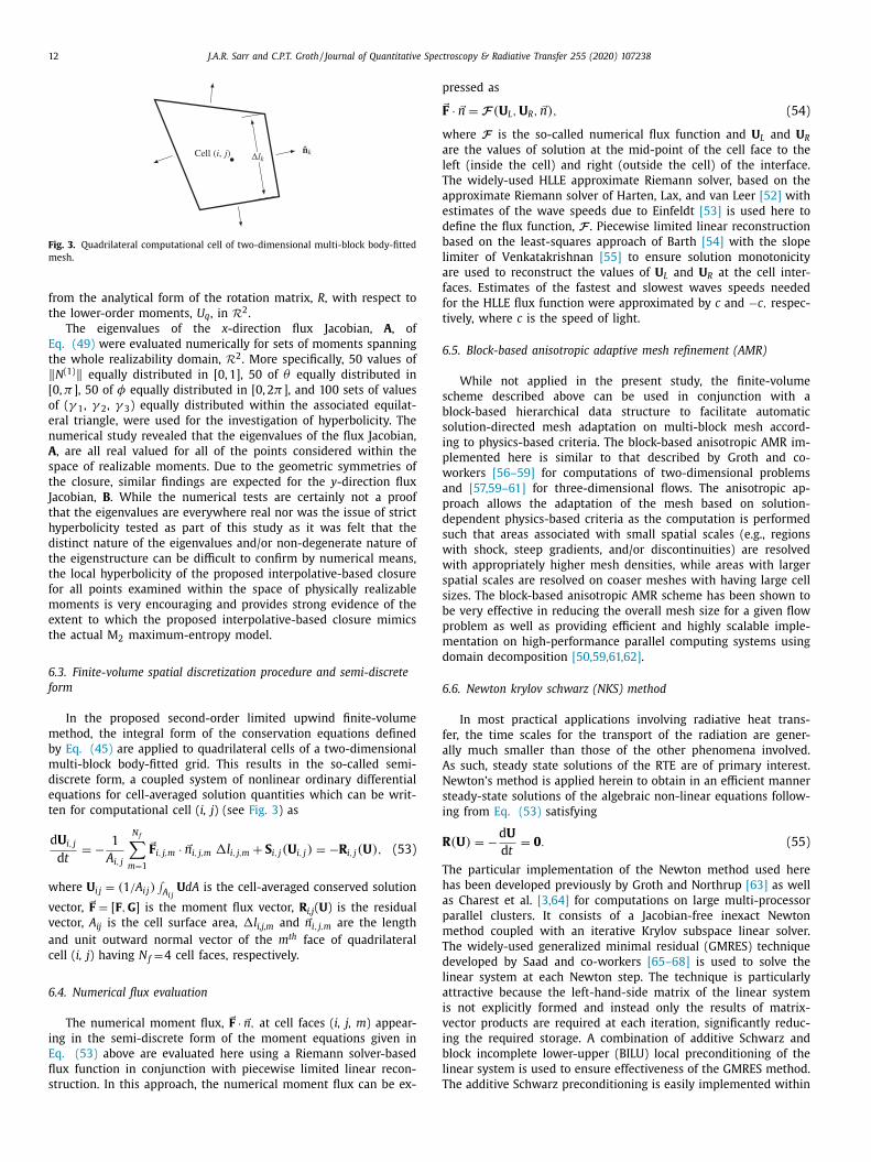
Fig. 3. Quadrilateral computational cell of two-dimensional multi-block body-fitted
mesh.
p
�F
w
a
l
T
a
e
d
b
l
a
f
f
t
6
s
b
s
i
p
w
a
p
d
s
w
w
s
s
b
p
m
d
6
f
a
A
N
s
i
R
T
h
a
p
m
T
d
l
a
i
v
i
b
l
T
from the analytical form of the rotation matrix, R , with respect to
the lower-order moments, U q , in R
2 .
The eigenvalues of the x -direction flux Jacobian, A , of
Eq. (49) were evaluated numerically for sets of moments spanning
the whole realizability domain, R
2 . More specifically, 50 values of
‖ N
(1) ‖ equally distributed in [0, 1], 50 of θ equally distributed in
[0, π ], 50 of φ equally distributed in [0, 2 π ], and 100 sets of values
of ( γ 1 , γ 2 , γ 3 ) equally distributed within the associated equilat-
eral triangle, were used for the investigation of hyperbolicity. The
numerical study revealed that the eigenvalues of the flux Jacobian,
A , are all real valued for all of the points considered within the
space of realizable moments. Due to the geometric symmetries of
the closure, similar findings are expected for the y -direction flux
Jacobian, B . While the numerical tests are certainly not a proof
that the eigenvalues are everywhere real nor was the issue of strict
hyperbolicity tested as part of this study as it was felt that the
distinct nature of the eigenvalues and/or non-degenerate nature of
the eigenstructure can be difficult to confirm by numerical means,
the local hyperbolicity of the proposed interpolative-based closure
for all points examined within the space of physically realizable
moments is very encouraging and provides strong evidence of the
extent to which the proposed interpolative-based closure mimics
the actual M 2 maximum-entropy model.
6.3. Finite-volume spatial discretization procedure and semi-discrete
form
In the proposed second-order limited upwind finite-volume
method, the integral form of the conservation equations defined
by Eq. (45) are applied to quadrilateral cells of a two-dimensional
multi-block body-fitted grid. This results in the so-called semi-
discrete form, a coupled system of nonlinear ordinary differential
equations for cell-averaged solution quantities which can be writ-
ten for computational cell ( i, j ) (see Fig. 3 ) as
d U i, j
d t = − 1
A i, j
N f ∑
m =1
� F i, j,m
· � n i, j,m
�l i, j,m
+ S i, j ( U i, j ) = −R i, j ( U ) , (53)
where U i j = (1 / A i j ) ∫
A i j U dA is the cell-averaged conserved solution
vector, � F = [ F , G ] is the moment flux vector, R i,j ( U ) is the residual
vector, A ij is the cell surface area, �l i,j,m
and
� n i, j,m
are the length
and unit outward normal vector of the m
th face of quadrilateral
cell ( i, j ) having N f =4 cell faces, respectively.
6.4. Numerical flux evaluation
The numerical moment flux, � F · � n , at cell faces ( i, j, m ) appear-
ing in the semi-discrete form of the moment equations given in
Eq. (53) above are evaluated here using a Riemann solver-based
flux function in conjunction with piecewise limited linear recon-
struction. In this approach, the numerical moment flux can be ex-
ressed as
· � n = F ( U L , U R , � n ) , (54)
here F is the so-called numerical flux function and U L and U R
re the values of solution at the mid-point of the cell face to the
eft (inside the cell) and right (outside the cell) of the interface.
he widely-used HLLE approximate Riemann solver, based on the
pproximate Riemann solver of Harten, Lax, and van Leer [52] with
stimates of the wave speeds due to Einfeldt [53] is used here to
efine the flux function, F . Piecewise limited linear reconstruction
ased on the least-squares approach of Barth [54] with the slope
imiter of Venkatakrishnan [55] to ensure solution monotonicity
re used to reconstruct the values of U L and U R at the cell inter-
aces. Estimates of the fastest and slowest waves speeds needed
or the HLLE flux function were approximated by c and −c, respec-
While not applied in the present study, the finite-volume
cheme described above can be used in conjunction with a
lock-based hierarchical data structure to facilitate automatic
olution-directed mesh adaptation on multi-block mesh accord-
ng to physics-based criteria. The block-based anisotropic AMR im-
lemented here is similar to that described by Groth and co-
orkers [56–59] for computations of two-dimensional problems
nd [57,59–61] for three-dimensional flows. The anisotropic ap-
roach allows the adaptation of the mesh based on solution-
ependent physics-based criteria as the computation is performed
uch that areas associated with small spatial scales (e.g., regions
ith shock, steep gradients, and/or discontinuities) are resolved
ith appropriately higher mesh densities, while areas with larger
patial scales are resolved on coaser meshes with having large cell
izes. The block-based anisotropic AMR scheme has been shown to
e very effective in reducing the overall mesh size for a given flow
roblem as well as providing efficient and highly scalable imple-
entation on high-performance parallel computing systems using
omain decomposition [50,59,61,62] .
.6. Newton krylov schwarz (NKS) method
In most practical applications involving radiative heat trans-
er, the time scales for the transport of the radiation are gener-
lly much smaller than those of the other phenomena involved.
s such, steady state solutions of the RTE are of primary interest.
ewton’s method is applied herein to obtain in an efficient manner
teady-state solutions of the algebraic non-linear equations follow-
ng from Eq. (53) satisfying
( U ) = −d U
d t = 0 . (55)
he particular implementation of the Newton method used here
as been developed previously by Groth and Northrup [63] as well
s Charest et al. [3,64] for computations on large multi-processor
arallel clusters. It consists of a Jacobian-free inexact Newton
ethod coupled with an iterative Krylov subspace linear solver.
he widely-used generalized minimal residual (GMRES) technique
eveloped by Saad and co-workers [65–68] is used to solve the
inear system at each Newton step. The technique is particularly
ttractive because the left-hand-side matrix of the linear system
s not explicitly formed and instead only the results of matrix-
ector products are required at each iteration, significantly reduc-
ng the required storage. A combination of additive Schwarz and
lock incomplete lower-upper (BILU) local preconditioning of the
inear system is used to ensure effectiveness of the GMRES method.
he additive Schwarz preconditioning is easily implemented within
J.A.R. Sarr and C.P.T. Groth / Journal of Quantitative Spectroscopy & Radiative Transfer 255 (2020) 107238 13
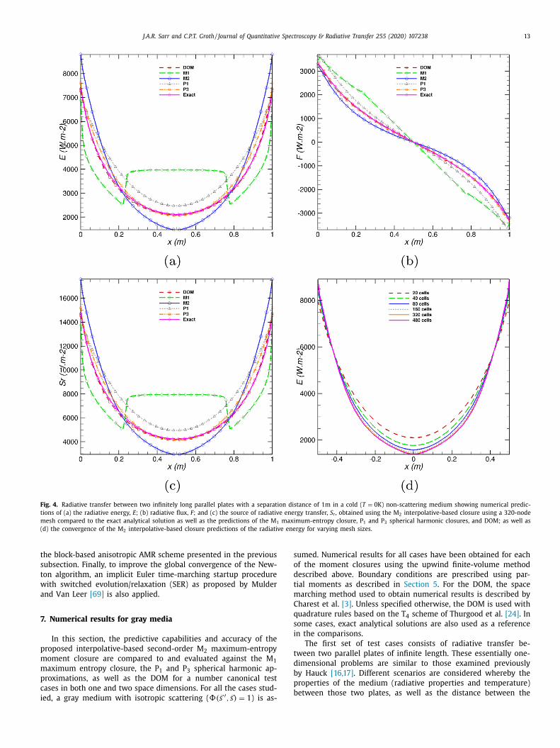
Fig. 4. Radiative transfer between two infinitely long parallel plates with a separation distance of 1m in a cold ( T = 0K ) non-scattering medium showing numerical predic-
tions of (a) the radiative energy, E ; (b) radiative flux, F ; and (c) the source of radiative energy transfer, S r , obtained using the M 2 interpolative-based closure using a 320-node
mesh compared to the exact analytical solution as well as the predictions of the M 1 maximum-entropy closure, P 1 and P 3 spherical harmonic closures, and DOM; as well as
(d) the convergence of the M 2 interpolative-based closure predictions of the radiative energy for varying mesh sizes.
t
s
t
w
a
7
p
m
m
p
c
i
s
o
d
t
m
C
q
s
i
t
d
b
p
b
he block-based anisotropic AMR scheme presented in the previous
ubsection. Finally, to improve the global convergence of the New-
on algorithm, an implicit Euler time-marching startup procedure
ith switched evolution/relaxation (SER) as proposed by Mulder
nd Van Leer [69] is also applied.
. Numerical results for gray media
In this section, the predictive capabilities and accuracy of the
roposed interpolative-based second-order M 2 maximum-entropy
oment closure are compared to and evaluated against the M 1
aximum entropy closure, the P 1 and P 3 spherical harmonic ap-
roximations, as well as the DOM for a number canonical test
ases in both one and two space dimensions. For all the cases stud-
ed, a gray medium with isotropic scattering ( �( � s ′ , � s ) = 1 ) is as-
umed. Numerical results for all cases have been obtained for each
f the moment closures using the upwind finite-volume method
escribed above. Boundary conditions are prescribed using par-
ial moments as described in Section 5 . For the DOM, the space
arching method used to obtain numerical results is described by
harest et al. [3] . Unless specified otherwise, the DOM is used with
uadrature rules based on the T 4 scheme of Thurgood et al. [24] . In
ome cases, exact analytical solutions are also used as a reference
n the comparisons.
The first set of test cases consists of radiative transfer be-
ween two parallel plates of infinite length. These essentially one-
imensional problems are similar to those examined previously
y Hauck [16,17] . Different scenarios are considered whereby the
roperties of the medium (radiative properties and temperature)
etween those two plates, as well as the distance between the
14 J.A.R. Sarr and C.P.T. Groth / Journal of Quantitative Spectroscopy & Radiative Transfer 255 (2020) 107238
Fig. 5. Radiative transfer between two infinitely long parallel plates with a separation distance of 10m in a cold ( T = 0 K) non-scattering medium showing numerical pre-
dictions of (a) the radiative energy, E ; (b) radiative flux, F ; and (c) the source of radiative energy transfer, S r , obtained using the M 2 interpolative-based closure using a
320-node mesh compared to the predictions of the M 1 maximum-entropy closure, P 1 and P 3 spherical harmonic closures and DOM; as well as (d) the convergence of the
M 2 interpolative-based closure predictions of the radiative energy for varying mesh sizes.
v
t
(
r
t
o
b
7
a
t
t
plates, are varied in order to assess the impact on the predictive
capabilities of the proposed M 2 closure. The first two-dimensional
test case consists of evaluating the accuracy of the M 2 closure in
predicting radiative heat transfer throughout a cold (non-emitting)
and absorbing medium contained within a square enclosure for
which all of the walls have the same temperature. Lastly, a line
source problem, which consists of a cold, non-scattering and
strongly absorbing medium, confined within a square computa-
tional domain, is also considered.
7.1. Parallel plates
As a first assessment of the proposed interpolative-based M 2
closure, radiative transfer between two hot parallel plates of infi-
nite length compared to their separation distance is studied. Two
ariants of this problem are considered. In the first variant of this
est case, the medium between the plates is assumed to be cold
non-emitting) non-scattering, and the predictions of the different
adiation models are compared for different plate separation dis-
ances. The second variant of this test case considers the effects
f scattering on the predictive capabilities of the M 2 interpolative-
ased closure.
.1.1. Exact solution for non-scattering case
For a non-scattering medium confined between two black, par-
llel plates, there exists an exact analytical solution to the radia-
ive transfer equation as given by Modest [1] . The distribution of
he radiative intensity emitted from the lower and upper plates are
J.A.R. Sarr and C.P.T. Groth / Journal of Quantitative Spectroscopy & Radiative Transfer 255 (2020) 107238 15
Fig. 6. Radiative transfer between two infinitely long parallel plates with a separation distance of 1m in a cold ( T = 0K ) scattering medium showing numerical predictions of
(a) the radiative energy, E ; (b) radiative flux, F ; and (c) the source of radiative energy transfer, S r , obtained using the M 2 interpolative-based closure using a 320-node mesh
compared to the predictions of the M 1 maximum-entropy closure, P 1 and P 3 spherical harmonic closures and DOM; as well as (d) the convergence of the M 2 interpolative-
based closure predictions of the radiative energy for varying mesh sizes.
g
I
I
r
t
a
I
m
a
s
2
E
F
w
L
f
iven by
+ (τ ′ , μ) = I w 1 e −τ/μ +
1
μ
∫ τ
0
I b (τ ′ ) e −(τ−τ ′ ) /μd τ ′ = I b + ( I w 1 − I b ) e
−τ/μ 0 < μ < 1 (56)
−(τ ′ , μ) = I w 2 e (τL −τ ) /μ − 1
μ
∫ τ
0
I b (τ ′ ) e (τ ′−τ ) /μd τ ′ = I b + ( I w 2 − I b ) e
(τL −τ ) /μ − 1 < μ < 0 (57)
espectively, where τL =
∫ L 0 β(s ) ds is the optical thickness (or op-
ical depth), L is the distance between the two plates, I w 1 and I w 2
re the intensities leaving the lower and upper plates respectively,
(τ ′ ) = I is the black-body radiative intensity distribution of the
b b
edium, and the substitution μ = cos θ is made to simplify the
nalysis.
Very accurate zeroth and first moments of the preceding exact
olutions of the radiative intensities can be achieved by using a
0-point Gauss-Legendre quadrature rule such that
± = ±2 π
∫ ±1
0
I ±(τ, μ)d μ = 2 π20 ∑
n =1
w n I ±(τ, μn ) (58)
± = ±2 π
∫ ±1
0
μI ±(τ, μ)d μ = 2 π20 ∑
n =1
w n μn I ±(τ, μn ) (59)
here the points μn and weights w n are determined by the Gauss-
egendre quadrature in the appropriate domains (i.e., μn ∈ [0, 1]
or lower plate and μn ∈ [ −1 , 0] for upper plate). The overall ra-
16 J.A.R. Sarr and C.P.T. Groth / Journal of Quantitative Spectroscopy & Radiative Transfer 255 (2020) 107238
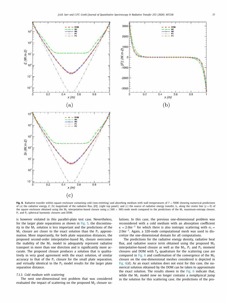
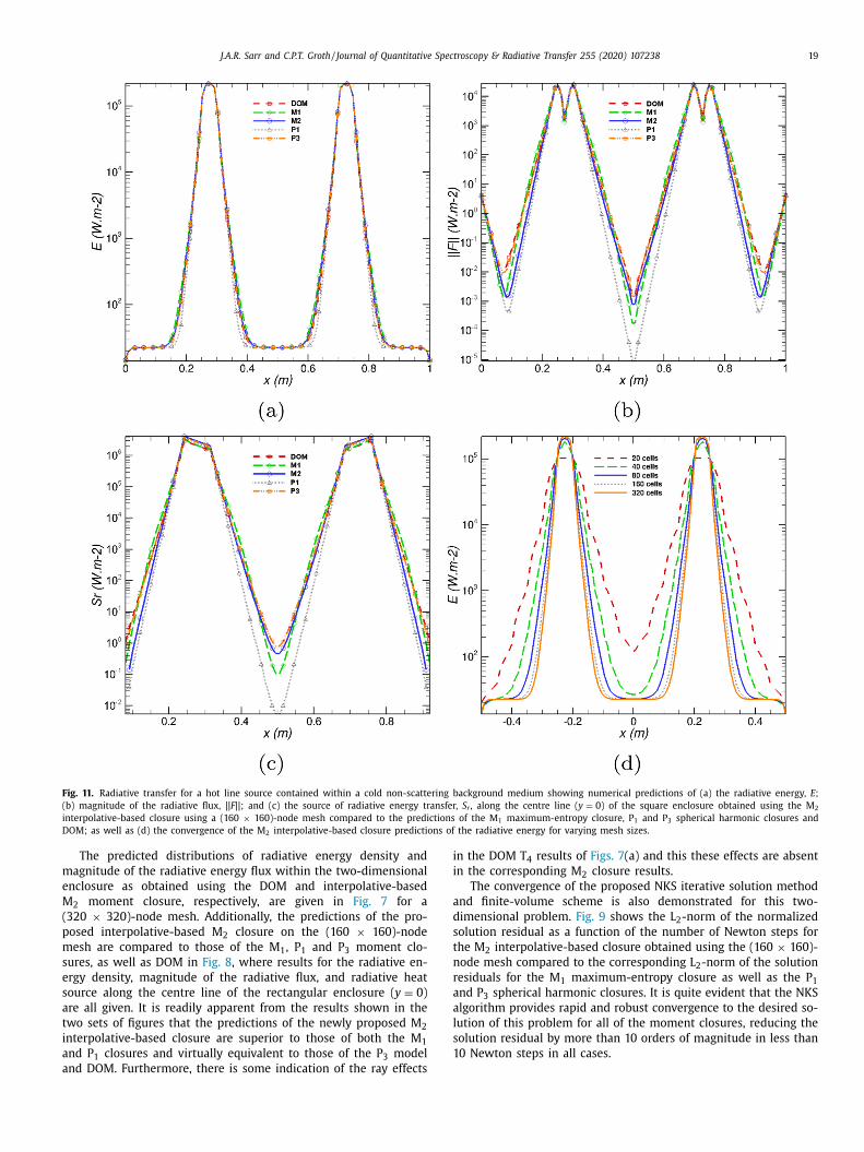
Fig. 7. Radiative transfer within square enclosure containing cold (non-emitting) and absorbing medium with wall temperatures of T = 500K showing numerical predictions
of the distribution of the radiative energy density using (a) the DOM & (b) the interpolative-based M 2 moment closure; the distribution of the magnitude of the radiative
energy flux as obtained using (c) the DOM & (d) our interpolative-based M 2 moment closure, on a (320 × 320)-node mesh.
g
i
m
l
a
e
t
F
m
I
d
s
s
t
t
i
diative energy at any optical distance, τ , between the two plates
is the sum of the radiative energy arising from both the lower and
upper plates. This sum also holds true for the overall radiative heat
flux.
7.1.2. Cold medium with no scattering
As a first test case, radiative transfer throughout a cold ( T =0K ), non-scattering medium with an absorption coefficient κ =2 m
−1 between two parallel plates was studied. Each of the plates
was taken to have a temperature of T = 500 K . The predictions
for the radiative energy density, radiative heat flux, and radiative
source term obtained using the proposed M 2 interpolative-based
closure as well as the M 1 , P 1 and P 3 moment closures and DOM
are compared for two plate separation distances: 1 and 10m as
shown in Figs. 4 and 5 , respectively. The predictions in all cases
were obtained using 320-node, uniformly-spaced, computational
mesh to discretize the space between the two plates. Conver-
ence of the interpolative-based M 2 closure solutions with increas-
ng mesh resolution ranging from 20- to 480-node computational
eshes are depicted in Figs. 4 (d) and 5 (d), confirming that the so-
utions are satisfactorily converged on the 320-node grid. The an-
lytical solution derived in Eqs. (58) and (59) , is used as a refer-
nce for the comparisons. Note that for both separation distances,
he DOM is observed to agree very closely with the exact solution.
For the small plate separation, it is readily apparent from
ig. 4 that the P N approximations (P 1 and P 3 ) yield somewhat
ore accurate predictions than the M 1 maximum entropy closure.
t can also be observed that the M 1 model produces a nonphysical
iscontinuity in the radiative energy. Previous analysis [14] have
hown that this jump is due to the inability of this first-order clo-
ure to handle radiative flux occurring in regions where bidirec-
ional radiative transfer is important. In fact, the closure condi-
ions for M 1 are derived under the assumption that the intensity
s symmetric about the direction of the flux. Such an assumption
J.A.R. Sarr and C.P.T. Groth / Journal of Quantitative Spectroscopy & Radiative Transfer 255 (2020) 107238 17
Fig. 8. Radiative transfer within square enclosure containing cold (non-emitting) and absorbing medium with wall temperatures of T = 500K showing numerical predictions
of (a) the radiative energy, E ; (b) magnitude of the radiative flux, || F ||, (right top panel); and (c) the source of radiative energy transfer, S r , along the centre line ( y = 0 ) of
the square enclosure obtained using the M 2 interpolative-based closure using a (160 × 160)-node mesh compared to the predictions of the M 1 maximum-entropy closure,
P 1 and P 3 spherical harmonic closures and DOM.
i
f
i
M
m
p
t
t
c
t
a
a
s
7
e
l
r
κ
2
c
fl
i
c
c
c
F
m
t
w
i
s however violated in this parallel-plate test case. Nevertheless,
or the larger plate separations as shown in Fig. 5 , the discontinu-
ty in the M 1 solution is less important and the predictions of the
1 closure are closer to the exact solution than the P 1 approxi-
ation. More importantly, for both plate separation distances, the
roposed second-order interpolative-based M 2 closure overcomes
he inability of the M 1 model to adequately represent radiative
ransport in more than one direction and is significantly more ac-
urate. The proposed closure produces a solution that is qualita-
ively in very good agreement with the exact solution, of similar
ccuracy to that of the P 1 closure for the small plate separation,
nd virtually identical to the P 3 model results for the larger plate
eparation distance.
.1.3. Cold medium with scattering
The next one-dimensional test problem that was considered
valuated the impact of scattering on the proposed M closure so-
2
utions. In this case, the previous one-dimensional problem was
econsidered with a cold medium with an absorption coefficient
= 2 . 0 m
−1 for which there is also isotropic scattering with σs = . 0 m
−1 . Again, a 320-node computational mesh was used to dis-
retize the one-dimensional domain for all computations.
The predictions for the radiative energy density, radiative heat
ux, and radiative source term obtained using the proposed M 2
nterpolative-based closure as well as the M 1 , P 1 and P 3 moment
losures and DOM with T 4 quadrature for the scattering case are
ompared in Fig. 6 and confirmation of the convergence of the M 2
losure on the one-dimensional meshes considered is depicted in
ig. 6 (d). As an exact solution does not exist for this case, the nu-
erical solution obtained by the DOM can be taken to approximate
he exact solution. The results shown in the Fig. 6 indicate that,
hile the M 1 model now no longer contains a nonphysical jump
n the solution for this scattering case, the predictions of the pro-
18 J.A.R. Sarr and C.P.T. Groth / Journal of Quantitative Spectroscopy & Radiative Transfer 255 (2020) 107238
Fig. 9. Convergence of the proposed NKS iterative solution method and finite-volume scheme for the problem of radiative transfer within square enclosure containing cold
(non-emitting) and absorbing medium with wall temperatures of T = 500 K showing the L 2 -norm of the normalized solution residual as a function of the number of Newton
steps for the M 2 interpolative-based closure using a (160 × 160)-node mesh compared to the corresponding L 2 -norm of the solution residuals for the M 1 maximum-entropy
closure as well as P 1 and P 3 spherical harmonic closures.
Fig. 10. Radiative transfer for a hot line source contained within a cold non-scattering background medium showing numerical predictions of the distributions of the
radiative energy density as obtained using (a) the DOM and (b) the interpolative-based M 2 moment closure, on a (320 × 320)-node mesh.
7
posed intepolative-based M 2 closure are significantly better than
those of both the M 1 and P 1 closures and lie very close to those
of both the P 3 closure and “exact” solution as represented by the
DOM results. w
c
t
.2. Square enclosure
The first two-dimensional test case considers a square enclosure
ith a cold (non-emitting) and absorbing medium. The absorption
oefficient was taken to be κ = 20 m
−1 . All of the walls are taken
o have identical temperatures of T = 500 K .
J.A.R. Sarr and C.P.T. Groth / Journal of Quantitative Spectroscopy & Radiative Transfer 255 (2020) 107238 19
Fig. 11. Radiative transfer for a hot line source contained within a cold non-scattering background medium showing numerical predictions of (a) the radiative energy, E ;
(b) magnitude of the radiative flux, || F ||; and (c) the source of radiative energy transfer, S r , along the centre line ( y = 0 ) of the square enclosure obtained using the M 2
interpolative-based closure using a (160 × 160)-node mesh compared to the predictions of the M 1 maximum-entropy closure, P 1 and P 3 spherical harmonic closures and
DOM; as well as (d) the convergence of the M 2 interpolative-based closure predictions of the radiative energy for varying mesh sizes.
m
e
M
(
p
m
s
e
s
a
t
i
a
a
i
i
a
d
s
t
n
r
a
a
l
s
1
The predicted distributions of radiative energy density and
agnitude of the radiative energy flux within the two-dimensional
nclosure as obtained using the DOM and interpolative-based
2 moment closure, respectively, are given in Fig. 7 for a
320 × 320)-node mesh. Additionally, the predictions of the pro-
osed interpolative-based M 2 closure on the (160 × 160)-node
esh are compared to those of the M 1 , P 1 and P 3 moment clo-
ures, as well as DOM in Fig. 8 , where results for the radiative en-
rgy density, magnitude of the radiative flux, and radiative heat
ource along the centre line of the rectangular enclosure ( y = 0 )
re all given. It is readily apparent from the results shown in the
wo sets of figures that the predictions of the newly proposed M 2
nterpolative-based closure are superior to those of both the M 1
nd P 1 closures and virtually equivalent to those of the P 3 model
nd DOM. Furthermore, there is some indication of the ray effects
n the DOM T 4 results of Figs. 7 (a) and this these effects are absent
n the corresponding M 2 closure results.
The convergence of the proposed NKS iterative solution method
nd finite-volume scheme is also demonstrated for this two-
imensional problem. Fig. 9 shows the L 2 -norm of the normalized
olution residual as a function of the number of Newton steps for
he M 2 interpolative-based closure obtained using the (160 × 160)-
ode mesh compared to the corresponding L 2 -norm of the solution
esiduals for the M 1 maximum-entropy closure as well as the P 1 nd P 3 spherical harmonic closures. It is quite evident that the NKS
lgorithm provides rapid and robust convergence to the desired so-
ution of this problem for all of the moment closures, reducing the
olution residual by more than 10 orders of magnitude in less than
0 Newton steps in all cases.
20 J.A.R. Sarr and C.P.T. Groth / Journal of Quantitative Spectroscopy & Radiative Transfer 255 (2020) 107238
C
V
W
s
A
G
S
(
r
e
t
c
g
t
l
a
t
s
A
r
t
N
t
m
o
m
R
T
t
w
N
w
w
t
t
s
t
t
∑
T
m
λ
a
∑
7.3. Line source problem
The last assessment of the predictive capabilities of the newly-
developed approximation of the gray M 2 closure considers a two-
dimensional line source problem, which consists of a cold, non-
scattering medium with an absorption coefficient κ = 100 m
−1
m
−1 , confined within a square computational domain. At the cen-
tre of the domain, there exists a hot line source at a temperature of
T = 1 , 0 0 0 K with inner radius 0.2 m and outer radius 0.25 m. Pre-
dictions of the distribution of the radiative energy density within
the enclosure, obtained using the DOM with T 4 quadrature and
the M 2 interpolative-based closure are compared in Fig. 10 for a
(320 × 320)-node mesh. Additionally, Fig. 11 compares the predic-
tions of the radiative energy, the magnitude of the radiative flux,
and the radiative energy source term along the y = 0 centre line
obtained using the proposed second-oder M 2 interpolative-based
closure to those of the M 1 , P 1 , and P 3 closures, as well as the DOM
with T 4 quadrature for a (160 × 160)-node computational mesh.
Grid convergence for this two-dimensional case is confirmed by
the results of a grid convergence study shown in Fig. 11 (d) for grids
ranging in size from (20 × 20) to (320 × 320) nodes. It is evident
from the results shown in the two figures that both the M 2 and
P 3 closures provide increased accuracy compared to their respec-
tive lower-order counterparts, i.e., the M 1 and P 1 models, respec-
tively. Moreover, as for the square enclosure problem, the predic-
tions of proposed M 2 interpolative-based closure are nearly iden-
tical to those of both the P 3 spherical harmonic closure and the
DOM, while involving considerably fewer unknowns or degrees of
freedom than either of the other two methods.
8. Conclusions
Inspired by the many desirable properties of maximum entropy
closures, a new, computationally-efficient, interpolative-based, M 2
moment closure has been proposed and developed for describing
radiative transport phenomena in gray media. Moment realizabil-
ity and hyperbolicity of the moment equations for the proposed
M 2 closure were both assessed. Unlike the interpolative-based M 2
closure proposed previously by Pichard et al . [19] , by construction
the present closure is valid for all physically realizable moments
sets up to second order and also appears to be globally hyperbolic.
The latter was shown numerically but not proven. Additionally, the
ability of the proposed M 2 closure to predict radiative heat transfer
in gray participating media for various one- and two-dimensional
canonical problems has been assessed by comparing predicted so-
lutions to those of other approximate techniques, including the M 1 ,
P 1 , and P 3 moment closures, as well as the DOM. The solutions of
the newly-proposed interpolative-based M 2 closure were observed
to be largely superior to those of either lower-order moment clo-
sures (i.e., the M 1 and P 1 models) and, at the very least, of equiva-
lent accuracy to the P 3 closure, while involving considerably fewer
angular moments (i.e., dependent variables). The proposed M 2 clo-
sure would seem rather promising and further investigation of the
interpolative closure would therefore seem warranted. Future re-
search will involve the extension of the interpolative-based M 2 clo-
sure to three-dimensional problems as well as the development of
a non-gray (spectrally dependent) M 2 closure, which will then be
validated for problems involving real-gas radiative transfer as en-
countered in reactive flows.
Declaration of Competing Interest
The authors have no competing interests to declare related to
manuscript submission.
RediT authorship contribution statement
Joachim A.R. Sarr: Conceptualization, Methodology, Software,
alidation, Formal analysis, Investigation, Writing - original draft,
riting - review & editing. Clinton P.T. Groth: Resources, Supervi-
ion, Writing - original draft, Writing - review & editing.
cknowledgements
This research was funded by grants and contracts from the
reen Aviation Research and Development Network (GARDN),
outhern Ontario Smart Computing for Innovation Platform
SOSCIP), as well as Pratt & Whitney Canada. The first author also
eceived support in the form of a scholarship from the Natural Sci-
nces and Engineering Research Council (NSERC) of Canada. Addi-
ionally, the computational resources for performing the numeri-
al simulations reported herein were provided by the SOSCIP pro-
ram as well as the SciNet High Performance Computing Consor-
ium at the University of Toronto and Compute/Calcul Canada (the
atter are funded by the Canada Foundation for Innovation (CFI)
nd Province of Ontario, Canada). Finally, the authors would like to
hank the two reviewers for their constructive criticisms and useful
uggestions for improving the clarity and quality of the revisions.
ppendix A. Necessary and sufficient conditions for
ealizability
Let us denote by R diag M 2
the rotation matrix which transforms
he coordinates system such that the second-order tensor N
(2) −
(1) (N
(1) ) T is diagonal. The necessary realizability conditions for
he moments in the new coordinate frame, with realizability do-
ain R
2 T , can then be derived from those for the moments in the
riginal frame, characterized by the realizability domain R
2 , by
eans of the transformation matrix, R diag M 2
, as follows
2 T ={ (I ′ (0) , I ′ (1) , I ′ (2) ) ∈ R
3 ×R
3×3 , s.t. I ′ (0) ≥ 0 , ‖ N
′ (1) ‖ ≤ 1 ,
N
′ (2) −N
′ (1) (N
′ (1) ) T ≥0 , (R diag M 2
� n ) T N
′ (2) (R diag M 2
) � n ≤1 ∀ ‖ � n ‖ ≤ 1 ,
tr(N
′ (2) ) = 1 and N
′ (2) i j
= N
′ (2) ji
} . he transformation from one set of moments to the other is illus-
rated in Eq. (31) . Since ( N
′ (2) i j
− N
′ (1) i
N
′ (1) j
) is diagonal, one can
rite
′ (2) i j
− N
′ (1) i
N
′ (1) j
= λi δi j
here λi correspond to the eigenvalues of ( N
′ (2) i j
− N
′ (1) i
N
′ (1) j
),
ith the associated eigenvector, � ηi , coinciding with the unit vec-
or along the coordinate axes with all entries equal to 0 except for
he i th entry which is equal to 1. Using the trace identity for the
econd-order moment, we can write
r(N
′ (2) i j
− N
′ (1) i
N
′ (1) j
) =
3 ∑
i =1
λi
r(N
′ (2) i j
) − tr(N
′ (1) i
N
′ (1) j
) =
3 ∑
i =1
λi
3
i =1
λi = 1 − ‖ N
(1) ‖
2
he latter identity can be further normalized by introducing nor-
J.A.R. Sarr and C.P.T. Groth / Journal of Quantitative Spectroscopy & Radiative Transfer 255 (2020) 107238 21
F
e
η
η
η
S
η
η
F
η
I
γ
A
t
u
d
a
h
l
f
∂
W
a
k
c
‖
∫
S
a
l
e
t
I
T
t
N
N
c
η
F
γ
w
i
A
N
I
∫
∫
∫
S
c
t
t
i
t
I
w
a
i
j
w
i
�s
a
o
I
urthermore, since � ηi is an eigenvector of ( N
′ (2) i j
− N
′ (1) i
N
′ (1) j
) with
igenvalue λi = (1 − ‖ N
′ (1) ‖ 2 ) γi , it follows that
(N
′ (2) − N
′ (1) (N
′ (1) ) T ) � ηi = λi � ηi
�
T i (N
′ (2) − N
′ (1) (N
′ (1) ) T ) � ηi =
� ηT i λi � ηi
�
T i (N
′ (2) − N
′ (1) (N
′ (1) ) T ) � ηi = λi � ηT i � ηi
�
T i (N
′ (2) − N
′ (1) (N
′ (1) ) T ) � ηi = λi ‖
� ηi ‖
ince � ηi is a unit vector, we have ‖ →
η i ‖ = 1 , and,
�
T i (N
′ (2) − N
′ (1) (N
′ (1) ) T ) � ηi = λi
�
T i (N
′ (2) − N
′ (1) (N
′ (1) ) T ) � ηi = (1 − ‖ N
′ (1) ‖
2 ) γi
rom the realizability conditions described above, we have
�
T i (N
′ (2) − N
′ (1) (N
′ (1) ) T ) � ηi ≥ 0 and ‖ N
′ (1) ‖ ≤ 1
t therefore follows that
i ≥ 0 , i = 1 , . . . , 3 . (A.2)
ppendix B. Form of the closure relation on the boundaries of
he realizability domain
On the boundaries of the realizability domain for moments
p to second-order, R
2 T , in multiple space dimensions, which we
enote ∂R
2 T , the inequality constraints on the normalized first-
nd second-order moments become sharp, and some or all of the
igher-order moments are uniquely determined in terms of the
ower-order moments. More specifically ∂R
2 T
can be written in the
orm
R
2 T = { (I ′ (0) , I ′ (1) , I ′ (2) ) ∈ R
3 × R
3 ×3 , s.t. I ′ (0) ≥ 0 ,
tr(N
′ (2) ) = 1 , N
′ (2) i j
= N
′ (2) ji
and ‖ N
′ (1) ‖ = 1
or (R diag M 2
� n ) T (N
′ (2) − N
′ (1) (N
′ (1) ) T )(R diag M 2
� n ) = 0 ∀
� n ∈ R
3 \ 0 or (R diag
M 2 � n ) T N
′ (2) (R diag M 2
� n ) = 1 ∀ ‖ � n ‖ ≤ 1 } .
(B.1)
e will now discuss the characteristics of each of the bound-
ries and also present the form of the distribution in terms of the
nown finite set of moments up to second-order.
In the case where ‖ N
′ (1) ‖ = 1 , which corresponds to the so-
alled free-streaming limit, we have
N
′ (1) ‖
2 = (N
′ (1) ) T N
′ (1) = 1
(N
′ (1) ) T ‖ I ′ (1) ‖
I ′ (0) = 1
(N
′ (1) ) T I ′ (1) = I ′ (0)
(N
′ (1) ) T ∫
4 π
� s Id� =
∫ 4 π
(N
′ (1) ) T � s Id� =
∫ 4 π
Id�
4 π(1 − (N
′ (1) ) T � s ) Id� = 0 .
ince the radiative intensity distribution is non-negative, i.e, I ≥ 0,
nd by definition 1 − (N
′ (1) ) T � s ≥ 0 , it therefore follows that the
atter equality holds if and only if the intensity distribution I is
qual to 0 everywhere except on the line � s = N
′ (1) , in which case
he distribution takes the form
= I (0) δ( � s − N
′ (1) ) . (B.2)
he form of the distribution in Eq. (B.2) can be integrated directly
o obtain analytical expression for N’ (3)
′ (3) i jk
= N
′ (1) i
N
′ (1) j
N
′ (1) k
. (B.3)
Let us now consider the case where (R diag M 2
� n ) T (N
′ (2) −
′ (1) (N
′ (1) ) T )(R diag M
� n ) = 0 ∀
� n ∈ R
3 \ 0 , and, in particular, the
2
ase where R diag M 2
� n =
� ηi , we then have
�
T i (N
′ (2) − N
′ (1) (N
′ (1) ) T ) � ηi = (1 − ‖ N
′ (1) ‖
2 ) γi = 0 .
or such relationship to hold for all ‖ N’ (1) ‖ ≤ 1, we must have
i = 0 ,
hich corresponds to one of the edges of the triangle (P 1 P 2 P 3 )
llustrated in Fig. 1 ; more specifically the edge (P j P k ), i � = j � = k .
long such an edge, we can write
′ (2) ii
− N
′ (1) i
N
′ (1) i
= 0 (B.4)
′ (2) ii
− N
′ (1) i
I ′ (1) i
= I ′ (2) ii
− 2 N
′ (1) i
I ′ (1) i
+
(I ′ (1) i
) 2
I ′ (0) = 0 (B.5)
4 πs 2 i Id� − 2 N
′ (1) i
∫ 4 π
s i Id� +
(I ′ (1) i
I ′ (0)
)2 ∫ 4 π
Id� = 0 (B.6)
4 π(s 2 i − 2 N
′ (1) i
s i + (N
′ (1) i
) 2 ) Id� = 0 (B.7)
4 π(�i − N
′ (1) i
) 2 Id� = 0 . (B.8)
ince I ≥ 0 and by definition (�i − N
′ (1) i
) 2 ≥ 0 , we can then con-
lude that the latter equality holds if and only if the intensity dis-
ribution I is equal to 0 everywhere except on the plane charac-
erized by s i = N ’ (1) i
. In the context of moment reconstruction us-
ng the principle of maximization of entropy, the distribution then
akes the form
=
δ(s i − N
′ (1) i
)
exp (αT m ( � s )) − 1
(B.9)
here the monomial basis for the angular moments, m ( � s ) , reads
s follows
• for i = 1
m ( � s ) =
[1 , �2 , �3 , �
2 2 , �2 �3
];
• for i = 2
m ( � s ) =
[1 , �1 , �3 , �
2 1 , �1 �3
];
• for i = 3
m ( � s ) =
[1 , �1 , �2 , �
2 1 , �1 �2
].
In the case where one of γ i , i = 1 , . . . , 3 , is equal to one as
s the case at the vertices of the triangle (P 1 P 2 P 3 ), then γ j = 0 ,
∈ {1, 2, 3} and j � = i , and from the findings in Eq. (B.4) , combined
ith the fact that � s is a unit vector, it follows that the distribution
s equal to zero everywhere except on the line
=
⎧ ⎪ ⎪ ⎪ ⎨
⎪ ⎪ ⎪ ⎩
(±√
1 − ‖ N
′ (1) ‖
2 + (N
′ (1) 1
) 2 , N
′ (1) 2
, N
′ (1) 3
) if γ1 = 1 ,
(N
′ (1) 1
, ±√
1 − ‖ N
′ (1) ‖
2 + (N
′ (1) 2
) 2 , N
′ (1) 3
) if γ2 = 1 ,
(N
′ (1) 1
, N
′ (1) 2
, ±√
1 − ‖ N
′ (1) ‖
2 + (N
′ (1) 3
) 2 ) if γ3 = 1 ,
(B.10)
nd the distribution is then uniquely determined by a Dirac delta
r a combination of Dirac deltas of the form
P i = I ′ (0) [ρ+
i δ(�i − x +
i ) + ρ−
i δ(�i − x −
i ) ]δ(� j − N
′ (1) j
) δ(�k − N
′ (1) k
) ,
(B.11)
22 J.A.R. Sarr and C.P.T. Groth / Journal of Quantitative Spectroscopy & Radiative Transfer 255 (2020) 107238
(
A
a
p
m
e
t
i
m
e
w
l
r
where ( i, j, k ) ∈ (1,2,3) with i � = j � = k and ρ+ i
, ρ−i
, x + i
and x −i
are
some parameters which must be determined from the realizablity
constraints for moments up to first-order (since the second-order
moments depend on the lower-order moments in this case), and
read as follows
x ±i
= ±√
1 − ‖ N
′ (1) ‖
2 + (N
′ (1) i
) 2 , and ρ±i
=
N
′ (1) i
− x ∓i
2 x ±i
.
(B.12)
Appendix C. Sufficiency of realizability conditions for moments
up to second-order
Let us consider a point P lying within the triangle (P 1 P 2 P 3 ) (see
Fig. 1 ) with corresponding set of moments ( I ′ (0) , I ′ (1) . I ′ (2) ), an re-
construct the distribution at the vertices of the triangle, given in
Eq. (B.11) , such that they exactly reproduce the zeroth and first-
order moments, I ′ (0) and I ′ (1) , respectively. We may then write the
distribution at the point P as a convex combination of the distri-
butions at the vertices of the triangle using the barycentric coordi-
nates, γ i , of the latter, as
I P =
3 ∑
i =1
γi I P i , (C.1)
From the above defined form of the distribution, it is clear, us-
ing Eq. (A.1) , that I P reproduces I ′ (0) and I ′ (1) , since I P i , i = 1 , . . . , 3
reproduce such moments. For the second-order moment, I ′ (2) , we
have
∫ 4 π
� s 2 I P d� =
3 ∑
i =1
γi
∫ 4 π
� s 2 I P i d�.
Computing the second-order moments at the vertices yields ∫ 4 π
�m
�n I P i d� = I ′ (0)
∫ 4 π
�m
�n
[ρ+
i δ(�i − x +
i )
+ ρ−i δ(�i −x −
i ) ]δ(� j −N
′ (1) j
) δ(�k −N
′ (1) k
) d�
∫ 4 π
�m
�n I P i d� = I ′ (0)
⎧ ⎪ ⎨
⎪ ⎩
ρ+ i
(x +
i
)2 + ρ−i
(x −
i
)2 if m = n = i, (
N
′ (1) m
)2 if m = n � = i,
N
′ (1) m
N
′ (1) n if m � = n,
For simplicity, we set I ′ (0) = 1 in the remainder of the derivation.
We will now distinguish two cases:
• Case 1: m � = n
∫ 4 π
�m
�n I P d� =
3 ∑
i =1
γi N
′ (1) m
N
′ (1) n ,
∫ 4 π
�m
�n I P d� = N
′ (1) m
N
′ (1) n
3 ∑
i =1
γi .
Using Eq. (A.1) , we then obtain ∫ 4 π
�m
�n I P d� = N
′ (1) m
N
′ (1) n . (C.2)
• Case 2: m = n = i ∫ 4 π
( �m
) 2 I P d� = γi
[ ρ+
m
(x + m
)2 + ρ−m
(x −m
)2 ]
+ γ j
(N
′ (1) m
)2 + γk
(N
′ (1) m
)2 , ∫
4 π( �m
) 2 I P d� = γi
[ (ρ+
m
+ ρ−m
) (x + m
)2 ]
+ γ j
(N
′ (1) m
)2 + γk
(N
′ (1) m
)2 .
From Eq. (B.12) , it is clear that ρ+ m
+ ρ−m
= 1 , and therefore Us-
ing Eq. (A.1) , we then obtain ∫ 4 π
( �m
) 2 I P d� = γi
(x + m
)2 + γ j
(N
′ (1) m
)2 + γk
(N
′ (1) m
)2 ,
∫ 4 π
( �m
) 2 I P d� = γi
(1 − ‖ N
′ (1) ‖
2 + (N
′ (1) m
) 2 )
+ γ j
(N
′ (1) m
)2
+ γk
(N
′ (1) m
)2 , ∫
4 π( �m
) 2 I P d� = (γi + γ j + γk )
(N
′ (1) m
)2 + γi
(1 − ‖ N
′ (1) ‖
2 ).
Again using Eq. (A.1) , we then obtain ∫ 4 π
( �m
) 2 I P d� =
(N
′ (1) m
)2 + γi
(1 − ‖ N
′ (1) ‖
2 )
(C.3)
From the results given in Eq. (C.2) and (C.3) , it is clear that I P with P ∈ R
2 T ), given in Eq. (C.1) also reproduces I ′ (2) .
ppendix D. Procedure for computing derivatives of the
ngular moments with respect to other angular moments
In our proposed interpolations, direct computation of the inter-
olating functions from the pre-computed solutions of the opti-
ization problem for entropy maximization yields undetermined
xpressions in the isotropic limit as well as on the boundaries of
he realizable domain. Applying l’Hopital’s rule is such cases results
n an expression in terms of the derivatives of the highest-order
oments with respect to the lower-order moments, which can be
xpressed as follows
∂ I (3)
∂ I ( j) =
9 ∑
i =0
∂ I (3)
∂αi
∂αi
∂ I ( j) , j = 0 , . . . , 2 , (D.1)
here we have used the chain rule for derivatives.
The derivatives of the Lagrange multipliers with respect to the
ower-order moments can be obtained by exploiting the following
elationships
∂ I (0)
∂ I (0) =
9 ∑
i =0
∂ I (0)
∂αi
∂αi
∂ I (0) = 1 ,
∂ I (0)
∂ I (1) j
=
9 ∑
i =0
∂ I (0)
∂αi
∂αi
∂ I (1) j
= 0 ,
∂ I (0)
∂ I (2) jk
=
9 ∑
i =0
∂ I (0)
∂αi
∂αi
∂ I (2) jk
= 0 , (D.2)
∂ I (1) j
∂ I (0) =
9 ∑
i =0
∂ I (1) j
∂αi
∂αi
∂ I (0) = 0 ,
∂ I (1) j
∂ I (1) k
=
9 ∑
i =0
∂ I (1)
∂αi
∂αi
∂ I (1) = δ jk ,
∂ I (1) j
∂ I (2) kl
=
9 ∑
i =0
∂ I (1) j
∂αi
∂αi
∂ I (2) kl
= 0 , (D.3)
∂ I (2) jk
∂ I (0) =
9 ∑
i =0
∂ I (2) jk
∂αi
∂αi
∂ I (0) = 0 ,
∂ I (2) jk
∂ I (1) l
=
9 ∑
i =0
∂ I (2) jk
∂αi
∂αi
∂ I (1) l
= 0 ,
∂ I (2) jk
∂ I (2) =
9 ∑
i =0
∂ I (2) jk
∂αi
∂αi
∂ I (2) = δ jl δkm
. (D.4)
lm lm
J.A.R. Sarr and C.P.T. Groth / Journal of Quantitative Spectroscopy & Radiative Transfer 255 (2020) 107238 23
l
H
w
H
a
A
a
a
A
R
[
[
[
[
[
[
[
[
[
[
[
[
[
[
[
[
[
[
[
[
[
[
The above relationships can be rewritten in matrix form as fol-
ows
A = I (D.5)
here
=
⎡
⎢ ⎢ ⎢ ⎢ ⎢ ⎢ ⎢ ⎢ ⎢ ⎢ ⎢ ⎢ ⎣
∂ I (0)
∂α1
∂ I (0)
∂α2 . . . ∂ I (0)
∂α9
∂ I (1) 1
∂α1
∂ I (1) 1
∂α2 . . .
∂ I (1) 1
∂α9
. . . . . . . . .
. . . ∂ I (1)
3
∂α1
∂ I (1) 3
∂α2 . . .
∂ I (1) 3
∂α9
∂ I (2) 11
∂α1
∂ I (2) 11
∂α2 . . .
∂ I (2) 11
∂α9
. . . . . . . . .
. . . ∂ I (2)
23
∂α1
∂ I (2) 23
∂α2 . . .
∂ I (2) 23
∂α9
⎤
⎥ ⎥ ⎥ ⎥ ⎥ ⎥ ⎥ ⎥ ⎥ ⎥ ⎥ ⎥ ⎦
(D.6)
nd
=
⎡
⎢ ⎢ ⎢ ⎢ ⎢ ⎢ ⎢ ⎢ ⎢ ⎢ ⎢ ⎢ ⎣
∂α1
∂ I (0)
∂α1
∂ I (1) 1
. . . ∂α1
∂ I (1) 3
∂α1
∂ I (2) 11
. . . ∂α1
∂ I (2) 23
∂α2
∂ I (0)
∂α2
∂ I (1) 1
. . . ∂α2
∂ I (1) 3
∂α2
∂ I (2) 11
. . . ∂α2
∂ I (2) 23
. . . . . . . . .
. . . . . .
. . . . . .
∂α4
∂ I (0)
∂α4
∂ I (1) 1
. . . ∂α4
∂ I (1) 3
∂α4
∂ I (2) 11
. . . ∂α4
∂ I (2) 23
∂α5
∂ I (0)
∂α5
∂ I (1) 1
. . . ∂α5
∂ I (1) 3
∂α5
∂ I (2) 11
. . . ∂α5
∂ I (2) 23
. . . . . . . . .
. . . . . .
. . . . . .
∂α9
∂ I (0)
∂α9
∂ I (1) 1
. . . ∂α9
∂ I (1) 3
∂α9
∂ I (2) 11
. . . ∂α9
∂ I (2) 23
⎤
⎥ ⎥ ⎥ ⎥ ⎥ ⎥ ⎥ ⎥ ⎥ ⎥ ⎥ ⎥ ⎦
(D.7)
nd I is a 9 × 9 identity matrix. The matrix A can then be written
s
= H
−1 . (D.8)
eferences
[1] Modest MF . Radiative heat transfer. 2nd. New York: Academic Press; 2003 . [2] W A Fiveland WA . Discrete-ordinates solutions of the radiative transport equa-
tion for rectangular enclosures. J Heat Transfer 1984;106(4):699–706 . [3] Charest MRJ , Groth CPT , Gülder ÖL . Solution of the equation of radiative trans-
fer using a newton-krylov approach and adaptive mesh refinement. J Comput
Phys 2012;231:3023–40 . [4] Grad H . On the kinetic theory of rarefied gases. Commun Pure Appl Math
1949;2:331–407 . [5] Jeans JH . The equations of radiative transfer of energy. Mon Not R Astron Soc
1917;78(1):28–36 . [6] Mazumder S , Modest MF . A probability density function approach to model-
ing turbulence-radiation interactions in nonluminous flames. Int J Heat Mass
Transf 1999;42(6):971–91 . [7] Li G , Modest MF . Importance of turbulence-radiation interactions in turbulent
diffusion jet flames. J Heat Transfer 2003;125(5):831–8 . [8] Modest MF , Mehta RS . Modeling absorption TRI in optically thick eddies. Pro-
ceedings of Eurotherm78 - Computational Thermal Radiation in ParticipatingMedia II 2006;78:225–34 .
[9] Gupta A , Modest MF , Haworth DC . Large-eddy simulation of turbulence-ra-
diation interactions in a turbulent planar channel flow. J Heat Transfer2009;131(6):061704–1–061704–8 .
[10] Menguc MP , Viskanta R . Radiative transfer in three-dimensional rectangu-lar enclosures containing inhomogeneous anisotropically scattering media. J
Quant Spectrosc Radiat Transfer 1985;33:533–49 . [11] Fletcher JK . The solution of the multigroup neutron transport equation using
spherical harmonics. Nucl Sci Eng 1983;84(1):33–46 .
[12] Dubroca B , Feugeas J-L . Theoretical and numerical study on a momentclosure hierarchy for the radiative transfer equation. SIAM J Numer Anal
1999;329:915–20 . [13] Jaynes ET . Information theory and statistical mechanics. Physical Review
1957;106:620–30 . [14] Brunner TA , Holloway JP . One-dimensional Riemann solvers and the maximum
entropy closure. J Quant Spectrosc Radiat Transfer 2001;69:543–66 . [15] Tencer J , Howell J . A parametric study of the accuracy of several radiative
transfer solution methods for a set of 2-D benchmark problems. In: Proceed-
ings of the ASME 2013 summer heat transfer conference, Minneapolis; 2013 . [16] Hauck CD . High-order entropy-based closures for linear transport in slab ge-
ometry. Report. Oak Ridge National Laboratory; 2010 . [17] Hauck CD . High-order entropy-based closures for linear transport in slab ge-
ometry. Commun Math Sci 2011;9(1):187–205 .
[18] Monreal P , Frank M . Higher order minimum entropy approximations in radia-tive transfer. arXiv Online Article. Cornell University Library; 2008 .
[19] Pichard T , Alldredge GW , Brull S , Dubroca B , Frank M . An approximation ofthe M 2 closure: application to radiotherapy dose simulation. J Sci Comput
2017;71(1):71–108 . 20] McDonald JG , Groth CPT . Towards realizable hyperbolic moment closures for
viscous heat-conducting gas flows based on a maximum-entropy distribution.Continuum Mech Thermodyn 2013;25:573–603 .
[21] McDonald JG , Torrilhon M . Affordable robust moment closures for CFD based
on the maximum-entropy hierarchy. J Comput Phys 2013;251:500–23 . 22] Kershaw D . Flux limiting nature’s own way. Technical Report. Lawrence Liver-
more Laboratory; 1976 . 23] Lathrop KD , Carlson BG . Discrete ordinates angular quadrature of the neutron
transport equation. Report LA. Los Alamos Scientific Laboratory; 1965 . [24] Thurgood CP , Pollard A , Becker HA . The T N quadrature set for the discrete or-
dinates method. ASME Journal of Heat Transfer 1995;117(4):1068–70 .
25] Coelho PJ . The role of ray effects and false scattering on the accuracy of thestandard and modified discrete ordinates methods. J Quant Spectrosc Radiat
Transfer 2002;73(2–5):231–8 . 26] Coelho PJ . Bounded skew high-order resolution schemes for the discrete ordi-
nates method. J Comput Phys 2002;175(2):412–37 . [27] Sakami M , El Kasmi A , Charette A . Analysis of radiative heat transfer in com-
plex two-dimensional enclosures with obstacles using the modified discrete
ordinates method. J Heat Transfer 2001;123(5):892–900 . 28] Koch R , Krebs W , Wittig S , Viskanta R . Discrete ordinates quadrature schemes
for multidimensional radiative transfer. J Quant Spectrosc Radiat Transfer1995;53(4):353–72 .
29] Ramankutty MA , Crosbie AL . Modified discrete ordinates solution of radiativetransfer in two-dimensional rectangular enclosures. J Quant Spectrosc Radiat
Transfer 1997;57(1):107–40 .
30] Amiri H , Mansouri SH , Coelho PJ . Application of the modified discrete ordi-nates method with the concept of blocked-off region to irregular geometries.
Int J Therm Sci 2011;50(4):515–24 . [31] Groth CPT , McDonald JG . Towards physically-realizable and hyperbolic moment
closures for kinetic theory. Continuum Mech Thermodyn 2009;21(6):467–93 . 32] Marshak RE . Note on the spherical harmonic method as applied to the milne
problem for a sphere. Physical Review 1947;71(7):443–6 .
[33] Arpaci VS , Gözüm D . Thermal stability of radiating fluids: the Bénard problem.Physics of Fluids 1973;16(5):581–8 .
34] Levermore C . Relating eddington factors to flux limiters. J Quant Spectrosc Ra-diat Transfer 1984;31(2):149–60 .
[35] Li R , Li W . 3D B 2 model for radiative transfer equation part I: modelling. Int JNumer Anal Model 2020;17(1):118–50 .
36] Monreal P . Moment realizability and Kershaw closures in radiative transfer.
RWTH Aachen University; 2012 . [37] Johnson S.G. The NLopt nonlinear-optimization package. http://github.com/
stevengj/nlopt ; 2014. 38] Kraft D . A software package for sequential quadratic programming. Technical
Report. Institut f ȭ r Dynamik der Flugsysteme, Oberpfaffenhof en; 1988 . 39] Kraft D . Algorithm 733; tomp—Fortran modules for optimal control calcula-
tions. ACM Trans Math Software 1994;20(3):262–81 . 40] Alldredge GW , Hauck CD , O’Leary DP , Tits AL . Adaptive change of basis in
entropy-based moment closures for linear kinetic equations. J Comput Phys
2014;258:489–508 . [41] Alldredge GW , Hauck CD , Tits AL . High-order entropy-based closures for lin-
ear transport in slab geometry II: a computational study of the optimizationproblem. SIAM Journal on Scientific Computing 2012;34(4):B361–91 .
42] Abramov RV . An improved algorithm for the multidimensional moment-con-strained maximum entropy problem. J Comput Phys 2007;226:621–44 .
43] Abramov RV . The multidimensional moment-constrained maximum en-
tropy problem: a BFGS algorithm with constraint scaling. J Comput Phys2009;228:96–108 .
44] Liu F , Swithenbank J , Garbett ES . The boundary condition of the P N approx-imation used to solve the radiative transfer equation. Int J Heat Mass Transf
1992;35(8):2043–52 . 45] Lax PD . Hyperbolic systems of conservation laws and the mathematical theory
of shock waves. CMBS–NSF Regional Conference Series in Applied Mathemat-
ics, 11. Philadelphia: SIAM; 1973 . 46] Levermore CD . Moment closure hierarchies for kinetic theories. J Stat Phys
1996;83:1021–65 . [47] Godunov SK . Finite-difference method for numerical computations of discon-
tinuous solutions of the equations of fluid dynamics. Matematicheskii Sbornik1959;47:271–306 .
48] Sachdev JS , Groth CPT , Gottlieb JJ . A parallel solution-adaptive scheme for pre-
dicting multi-phase core flows in solid propellant rocket motors. Int J ComutFluid Dyn 2005;19(2):159–77 .
49] Gao X , Groth CPT . A parallel adaptive mesh refinement algorithm for pre-dicting turbulent non-premixed combusting flows. Int J Comut Fluid Dyn
2006;20(5):349–57 . 50] Gao X , Northrup SA , Groth CPT . Parallel solution-adaptive method for two-di-
mensional non-premixed combusting flows. Progress in Computational Fluid
Dynamics 2011;11(2):76–95 . [51] McDonald JG , Sachdev JS , Groth CPT . Application of Gaussian moment closure
to micro-scale flows with moving and embedded boundaries. AIAA Journal2014;51(9):1839–57 .
finement for three-dimensional inviscid and viscous flows. Paper. AIAA; 2015 . [60] Freret L , Ivan L , De Sterck H , Groth CPT . High-order finite-volume method
with block-based AMR for magnetohydrodynamics flows. J Sci Comput2019;79(1):176–208 .
[61] Freret L, Williamsche M, Groth C.P.T. Parallel anisotropic non-uniform block-based adaptive mesh refinement for three-dimensional inviscid and viscous
flows. submitted to the Journal of Computational Physics; 2020.
[62] Gao X , Groth CPT . A parallel solution-adaptive method for three-di-mensional turbulent non-premixed combusting flows. J Comput Phys
2010;229(5):3250–75 . [63] Groth CPT , Northrup SA . Parallel implicit adaptive mesh refinement scheme for
[65] Saad Y , Schultz MH . GMRES: a generalized minimal residual algorithm for
solving nonsymmetric linear equations. SIAM Journal for Scientific and Statis-tical Computing 1986;7(3):856–69 .
[66] Saad Y . Krylov subspace methods on supercomputers. SIAM Journal for Scien-tific and Statistical Computing 1989;10(6):1200–32 .
[67] Brown PN , Saad Y . Hybrid Krylov methods for nonlinear systems of equations.SIAM Journal for Scientific and Statistical Computing 1990;11(3):450–81 .
[68] Saad Y . Iterative methods for sparse linear systems. Boston: PWS Publishing
Company; 1996 . [69] Mulder WA , van Leer B . Experiments with implicit upwind methods for the