Page 1
EFFECTS OF WEIGHTLESSNESS ON THE VESTIBULO-OCULAR REFLEX
IN THE CREW OF SPACELAB 1
by
MARK JOHN KULBASKI
SUBMITTED TO THE DEPARTMENT OFMECHANICAL ENGINEERING IN PARTIAL
FULFILLMENT OF THEREQUIREMENTS FOR THE
DEGREE OF
BACHELOR OF SCIENCE
at the
MASSACHUSETTS INSTITUTE OF TECHNOLOGY
June 1986
Q) MASSACHUSETTS INSTITUTE OF TECHNOLOGY 1986
Signature of Authof I "% - artment o4bMechanical Engineering
Ao May 16, 1986
Certified by__
Accepted by
Charles M. OmanThesis Supervisor
Peter GriffithChairman, Department Committee
Page 2
MIT LibrariesDocument Services
Room 14-055177 Massachusetts AvenueCambridge, MA 02139Ph: 617.253.2800Email: [email protected] ://libraries.mit.edu/docs
DISCLAIMER OF QUALITY
Due to the condition of the original material, there are unavoidableflaws in this reproduction. We have made every effort possible toprovide you with the best copy available. If you are dissatisfied withthis product and find it unusable, please contact Document Services assoon as possible.
Thank you.
Some pages in the original document contain pictures,graphics, or text that is illegible.
owl
Page 3
2
EFFECTS OF WEIGHTLESSNESS ON THE VESTIBULO-OCULAR REFLEX
IN THE CREW OF SPACELAB 1
by
MARK JOHN KULBASKI
Submitted to the Department of Mechanical Engineeringon May 16, 1986 in partial fulfillment of the
requirements for the Degree of Bachelor of Science inMechanical Engineering
ABSTRACT
Slow phase angular eye velocity during a post rotational vestibulo-ocular reflex (PVOR) was studied pre and post flight in the crew ofSpacelab 1, which orbited the earth for ten days in November, 1983. Sixsubjects were tested preflight. Four of those six flew on the missionand were tested postflight. Two separate vestibulo-ocular tests wereperformed.
First, subjects sat with the head upright in a chair that couldrotate about the earth vertical axis. The chair was rotated at 120degrees per second and then suddenly stopped. Eye movements wereanalyzed for 38 seconds after the stop. Subjects were tested in theclockwise and counterclockwise directions. Second, subjects were rotatedat 120 degrees per second as before. However, they tilted the head down5 seconds after the chair stopped and brought the head upright tenseconds after the chair stopped. Tests were carried out in bothdirections.
Slow phase eye velocity20 seconds were fit to a firLikewise, head down velocito first order models. Thestandard deviation obtainefive preflight days was 11.7constant was 3.2 +/- 0.8The mean postflight head uppopulation responses o er
profiles of the PVOR head up tests from 1 tost order model with time constant and gain.ty profiles between 5 and 10 seconds were fitmean preflight head up time constant +/- ond by averaging mean population responses over
+/- 0.9 seconds. The head down timeseconds. The gain was 0.59 +/- 0.1 seconds.
time constant obtained by averaging meanthe first two test days after landing was 9.3
+/- 0.3 seconds. The. head down time constant was.3.4 +/- 1.5 seconds.The gain was 0.60 +/- 0.03 seconds. a
A chi-squared test indicated that preflight vs postflight head upvelocity decay profiles were significantly different between six andtwenty seconds after the chair was stopped. Chi-squared tests indicatedthat both the pre and post flight head up and head down response profileswere significantly different between 5 and 10 seconds, respectively.
Thesis Supervisor: Dr. Charles M. OmanTitle: Senior Research Engineer of Aeronautics and Astronautics
Page 4
3
ACKNOl 3IMENTS
I wish to express my gratitude to my thesis advisor, Dr. Charles M.
Oman, for his guidance, insight, and sustained encouragement during the
course of this work. I also thank Sherry Modestino for invaluable
support on the MVL computer system, Dr. Alan Natapoff for helpful
criticisms on the statistical analysis, and Brian Rague for helping to
produce the plots. Eve Risk in's careful documen tation of the raw data
made this investigation possible.
This thesis is dedicated to my father and mother.
(
Page 5
4
Table of Contents
Page Number
Ti tle Page
Abstract
Acknowledgments 3
Table fo Contents 4
List of Figures 6
List of Tables 8
Chapter 1 Introduction 9
Chapter 2 Background 10
2.1 Physiology and physics of the vestibulo-ocular system 10
2.2 Per rotatory and post rotatory nystagmus 14
2.3 The central velocity storage element 15
2.4 Gravireceptor influence on the PVOR 17
2.5 Modeling the tilt suppression of nystagmus 19
Chapter 3 Experimental Procedure 22
Chapter 4 Data Processing 25
4.1 Overview of data processing 25
4.2 Detection of slow phase movements 25
4.3 Criteria for correcting mistakes of the algorithm 30
4.4 Criteria for discarding files 32
Chapter 5 Strategies for Analyzing the Data 35
5.1 Two statistical methods for analyzing PVOR data 35
5.2 Combining clockwise and counterclockwise responses 35
Chapter 6 Modeling slow phase eye velocity during a PVOR 41
Chapter 7 Results 45
7.1 Mean PVOR responses of individuals 45
Page 6
5
7.2 Mean daily responses of the population 55
7.3 Global response of the population -;
Chapter 8 Discussion 6.
Appendix I Suggestions for Other Experiments 71
Appendix II Listing of Programs 73
References 92
Page 7
6
List of Figures
2.2.1 Effects of a pulse angular velocity applied to the head 14
2.3.1 States of Vestibular organs in response to a step head 16angular velocity
2.5.1 Canal-otolith-oculomotor system models 20
4.2.1 Typical output of the Massoumnia algorithm 26
4.2.2 EOG and raw eye velocity plotted against time 27
4.2.3 EOG and corrected slow phase eye velocity plotted against time 29
4.2.4 Slow Phase Velocity Profile sample at 4 Hz 30
4.3.1 Schematic of a poor PVOR interpolation 31
4.4.1 High performance example of the Massoumnia algorithm 34
4.4.2 Low performance example of the Massoumnia algorithm 34
6.1.1 Global preflight head up PVOR profile 42
6.1.2 Model fit of the mean preflight head up PVOR 43
7.1.2 Results of individual subject model fits 48
7.1.3 Mean preflight and postflight head up and tilt suppression 51responses of subject 1
7.1.4 Mean preflight and postflight head up and tilt suppression 52responses of subject 2
7.1.5 Mean preflight and postflight hear! p and tilt suppression 53responses of subject 3
7.1.6 Mean preflight and postflight head up and tilt suppression 54responses of subject 4
7.2.2 Results of model fits to mean PVOR responses per test day 57
7.3.1 Global mean preflight PVOR profile with/without tilt 59suppression
7.3.2 Natural log of the global mean preflight PVOR profile 60with/without tilt suppression
7.3.3 Model fits for global preflight head up and head down 61responses
7.3.4 Global mean postflight PVOR profile with/without tilt 62
Page 8
7
suppression
7.3.5 Model fits of global postilght head up and head down 6responses
7.3.6 G!oba mean pre and post 41ight head up PVOR responses in 5linear-lInear and In-linear form
4
Page 9
S
List o+ Tables
7.1.1 Results of model fits for individual subjects averaged 45across testing days
7.2.1 Results of model fits for testing days averaged across 56indi v dual subjects
Page 10
9
Chapter 1
Introduction
The purpose of this investigation was to study how adaptation to
weightlessness affects the vestibulo-ocular system. The dynamics of post
rotational slow phase eye velocity were examined preflight and postflight
in the crew of Spacelab 1, which orbited the earth for ten days in
November, 1983. Subjects were tested both with the head upright and with
the head tilted forward five seconds after a step angular velocity from
120 degrees per second to 0 degrees per second about the vertical axis
was appiied to the head.
Benson and Bodin (1966) have shown that the apparent time constant
of post rotational slow phase velocity is sensitive to the body's
orientation to the gravity vector. In particular, they reported that the
apparent time constant was less when the head and body were pitched
forward or back than when the head and body remained upright. This
suggests that the brain weighs information from both the otoliths or
other gravireceptors with information from the semicircular canals to
estimate angular head velocity.
The vestibulo-ocular system may adapt to weightlessness by
reweighting or unweighting information from the gravireceptors. The
brain may, in general reinterpret all sensory cues about body dynamics in
weightlessness. Although control system engineers and physiologists have
modeled how the inner ear can control eye movements, and anatomists have
mapped basic neural pathways to support these models (Wilson and Jones,
1979), the vestibulo-ocular system is still not fully understood.
This study specifically documents preflight and postflight head up
Page 11
10
and head down post rotational slow phase eye velocity to learn more about
the structure and function of the vestibulo-ocular system by examining
how it adapts to weightlessness.
Work required to complete this thesis involved processing
experimental data which was recorded around the space flight, fitting the
data to models, and analyzing the results.
A secondary result of this project was to test the performance of
new digital filtering software which strips slow phase eye velocity from
a signal of eye position. The algorithm was developed by Mohammed-Ali
Massoumnia for a Master's Degree in Aeronautics and Astronautics at
M.I.T. in 1983. In the past, oculomotor research routinely required
processing large amounts of data by hand because no computer system was
as accurate as a trained human to analyze a complicated electooculography
(EOG) signal. This project would not have proceeded as quickly or as
accurately without the new software.
1 .4
Page 12
11
Chapter 2
Background
2.1 Physiology and physics of the vestibulo-ocular system
Organs in the inner ear which detect motion are part of the
"vestibular system." Muscles and their controllers which move the eyes
are part of the "oculornotor system." The vestibulo-ocular reflex (VOR)
refers to the phenomenon in which organs of the inner ear drive eye
movement. If the angular velocity of the eyes were equal in magnitude
and opposite in sign to the angular velocity of the head, there would be
no retinal vision blur when the head moved. For the image of a target to
remain stationary on the retina, the eyes must move as far and as quickly
as does the head, though they must move in the opposite direction. Thus,
to reduce ,ision blur during head rotation, the brain must measure the
dynamics of head movement and then calculate appropriate compensatory eye
movements.
Although the vestibular system does not directly measure head
angular velocity or position, the semicircular canals serve as pseudo
integrating angular accelerometers. There are three orthogonal
semicircular canals on either side of the head. Each is filled with a
fluid called endolymph, with properties similar to water. Angular
acceleration of the head produces motion of the endolymph with respect to
the canal walls, due to the inertia of the fluid. Displacement of the
endolymph deforms a gelatinous structure called the cupula, which
stimulates hair cells beneath it synapsing with afferent nerves. Fzr
brief head movements, distortion of the cupula produces negligible
pressure forces on the ring of endolymph, compared to large viscous drag
Page 13
12
from shear on the canal walls. Velocity of endolymph flow is
proportional to accelerat ion of the head and cupula position is
proportional to head velocity (Oman 1985).
Steinhausen (1931) and Van Egmond, et al (1949) have modeled the
cupula-endolymph relation as a simple second order system with
characteristic equation:
& 9where is the moment of inertia of the endolymph ring about the center
of the torus, 7r is the viscous drag coefficient of the endolymph on the
canal wall, A is the stiffness of the cupula, , is the deformation of
the cupula, and to is the angular position of the head. In the Laplace
frequency domain, the transfer function of the system is:
__s_ -U/
-e(s)
This can be approximately factored as
(T) -
0 6o ~r( ( f s+y)
Page 14
13
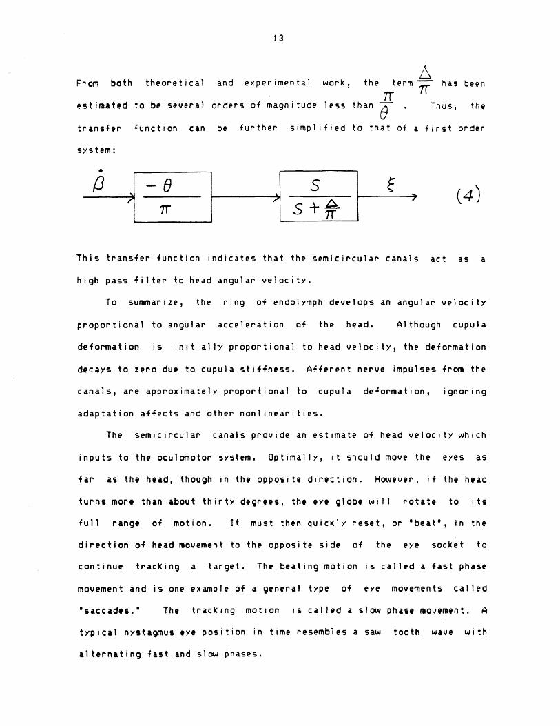
From both theoretical and experimental work, the term
ITestimated to be several orders of magnitude less than -
transfer function can be further simplified to that of a
system:
I5 -O S
Th is
high
transfer function indicates that the semicircular canals
pass filter to head angular velocity.
To summarize, the ring of endolymph develops an angu
7 - has been
Thus, the
first order
(4%)
act as a
lar velocity
proportional to angular acceleration
deformation is initially proportiona
decays to zero due to cupula stiffness
canals, are approximately proportional
adaptation affects and other nonlinear
The semicircular canals provide
inputs to the oculomotor system. Opti
far as the head, though in the opposi
turns more than about thirty degrees,
full range of motion. It must th
of the head. Although
1 to head velocity, the def
Afferent nerve impulses
to cupula deformation,
ities.
an estimate of head veloci
mally, it should move the
te direction. However, if
the eye globe will rotate
en quickly reset, or "beatu
direction of head movement to the opposite side of the eye socket to
continue tracking a target. The beating motion is called a fast phase
movement and is one example of a general type of eye movements called
"saccades.m The tracking motion is called a slow phase movement. A
typical nystagmus eye position in time resembles a saw tooth wave with
alternating fast and slow phases.
cupul a
ormation
from the
ignoring
ty wh
eyes
the h
to
in
ich
as
ead
its
the
Page 15
14
The sign of fast phase velocity is the negative of the sign of slow
phase velocity, the amplitude of last phase velocity is much greater than
the amplitude of slow phase velocity, and the duration of a fast phase
movement is much less than the duration of a slow phase movement. The
mean angular position of the eyes during nystagmus is approximately zero.
2.2 Per rotatory and post rotatory nystaqmus
Consider the effect of a square pulse angular velocity applied to
the head, as shown in Figure 2.2.1.
AngularHeadVelocity
Slow PhaseAngular EyeVelocity
Effect of square pulse angular velocityapplied to the head
Fig-2.2. 1
At time T1, an acceleration impulse deforms the cupula, which then
decays back to its resting position. The vestibular system drives the
slow phase eye velocity with a characteristic time constant and gain.
Slow phase eye movements are in the opposite direction of head movements
to keep a target in view.
At time T2, eye movements have stopped and the subject feels that he
Page 16
15
is not rotating. However, the acceleration impulse at time T2 driVes
slow phase movements in the opposite direction as before and the subjeCt
feels that he is rotating even though he remains still. Eye movement
curing head rotation is referred to as per rotatory-n-stagmus. Eye
movement after head rotation is referred to as post rotational nystagmus
or a post rotatory vestibulo-ocular reflex (PVOR).
2.3 The central velocity storage element
Experiments which measured afferent
semicircular canals of monkeys have suggested
constant
Fernandez
simi 1 ar,
veloc ity
of the
1971).
cupu 1 a
because
an apparent time const
Robinson (1977)
explain the apparent
integrates afferent
system. Although anat
element, Raphan and
storage element which
The phenomenon of
a central integrator.
tracking movements. H
stops, suggesting th
monkey cupula is about fi
Assuming human and monkey v
deformation alone probably does
human post rotatory slow phase
ant o
and
stre
canal
om i st
f about twenty
Raphan and
tched time c
signals bef
s have not co
seconc
Cohen
onstant
ore th
nclusiv
Cohen hypothesize that there
holds an est
optok inetic
A moving v
owever, the
at the mov
nerve signals from the
that the dominant time
ve seconds (Goldberg and
estibular physiology is
not drive slow phase eye
eye velocity decays with
s. (Malcolm, 1973)
(1985) have attempted to
with an element that
ey reach the oculo-motor
ely identified such an
is a central velocity
imate of angular head velocity.
after pystagmus supports the theory of
isual field will induce smooth eye
tracking continues even after the scene
ing field charged the state of the
integrator.
Figure 2.3.1 shows a sketch of the hypothesized states of the
Page 17
16
horizontal canal, the central integrator, and the oculomotor system
during a PVOR.
3 1) SEMICIRCULAR CANALS
2) CENTRAL VELOCITY STORAGE
AFFERENT 2ELEMENTOUTPUT 3) SLOW PHASE EYE VELOCITY
50 20 TIME (SEC)
States of vestibular organsin response to a step head \angular velocity
Fig-2.3.1
At time 0+, the cupula deforms. The afferent output decays quickly,
but this signal charges the the central integrator. If the oculomotor
system receives the outputs of both the canals and the integrator, then
slow phase velocity is proportional to the sum of the states of the canal
and the integrator and thus the effective time constant is stretched and
approximates the leak time constant of the integrator after about five
seconds.
Characterizing how this integrator affects slow phase angular eye
velocity may be central to interpreting the results of this
investigation. The state of the neural integrator may depend on
Page 18
17
information from the gravireceptor.
2.4 Gravireceptor influence on the PVOR
The otoliths are organs located near the semicircular canals and
provide an estimate of linear acceleration and head tilt. They contain
calcium crystals which are embedded in a membrane. Linear acceleration
shears the crystals over the membrane and stimulates hair cells beneath
it. The otoliths can measure the angle of head pitch, or tilt, because
the component of the gravity vector which shears the crystals over the
membrane changes in magnitude with the angle of head position.
Consider the conflicting information coming from the semicircular
canals and the otol
rotational test. The
when it stopped rotati
iths when the
horizontal angu
ng stimulated
pitching the head forwar
previously the roll axis.
head is rolling about an ea
vertical axis. However, th
and do not confirm that
information about body
proprioceptors, so we ca
from the canals and the oto
velocity to properly drive
Presumably,
head
lar acc
the ho
d translated th
Thus, the canals
rth horizontal ax
e otoli ths measur
the head is
position from
nnot assume that
liths when formin
slow phase eye ve
the brain has learned over
pitches
e 1 erat i o
r i zontal
e yaw
inform
is, not
e a stat
rolling.
other
the brai
g an est
loci ty.
forward
n impul
canal
axis
the br
yawing
ionary
The
organ
during a post
se to the head
s. However,
nto what was
ain that the
about an earth
gravity vector
brain receives
s, such as
n only weighs
imate of head
time that although th
signals
angu I ar
e head
constantly twists and p
not change direction.
information from grav
itches and rolls, the gravity vector probably does
Thus, during head tilt the brain probably weighs
ireceptors more than information from the
Page 19
18
semicircular canals. Benson- and Bodin's data supports the assumption
because it shows that post rotational slow phase eye velocity decayed
more quickly when the body pitched forward or back than when
upright. Slow
system's best
There is
gravireceptors
would learn
adaptation to
readaption to
be instantaneo
tests during t
What ad
possibilities.
information f
structures, th
during head t
adaptation to
dramatic phys
learned durin
information e
provide an ove
Changes i
because it
semicircular c
consistently
phase eye velocity
estimate of head angul
no gravity vect
when the body tilts,
to weigh signals fr
weightlessness takes s
gravity when the spac
presumably ref
ar velocity.
or in weightl
so it seems li
om this organ
everal days,
elab crew retur
lects the
essne
ke 1 y
I es
it i
ned t
it remained
vestibular
ss to stimulate
that the brain
s in space. If
s possible that
o earth would not
us and adaptation effects could be measured in vestibular
he first few days pos
aptation effects
If adaptation to
rom gravireceptors
en slow phase eye vel
ilt as quickly postfl
weightlessness involv
iological changes,
g weightlessness
ven more postflight
rwhelmingly strong cu
n th
is
e apparent
not clear
anals. If on
influenced
head
if
ear th
by
u
g
tf i
are
we
due
oc i t
ight
ed h
the
and
th
e fo
p ti
ravi
gh t.
expected?
ghtlessness
to physica
y is not
as it did
igher level
brain may
instead
an prefligh
r body posi
me constant
ty affects
the state of the
gravireceptors,
There
involved
,I changes
expected
preflight.
learning
quickly ig
weight g
t because i
tion.
are harder
the phys
cen
and
tral
if
are several
unweighting
n vestibular
to decrease
However, if
instead of
nore what it
ravireceptor
"rity would
to
cs
predict
of the
integrator is
in space,
gravireceptors are dormant, perhaps the brain would begin to mistrust the
(
i
Page 20
19
state of the integrator because it would not normally change with head
movements, as it would on the ground. Perhaps cupula afferent signals
would be weighted more than on the ground compared to central integrator
afferent signals, and the time constant of slow phase velocity would
approach more the short time constant of the cupula. The brain might
also learn to trust the visual system for cues about body position more
in space than on earth because the vestibular system would instantly give
different information from what the brain has learned to expect on the
ground. Thus the brain may increase the leak rate of the central
integrator because the brain does not want to hold what it is learning to
perceive as inaccurate information. This would also make postrotatory
slow phase velocity decay more quickly postflight than preflight.
2.5 Modeling the tilt suppression of nystagmus
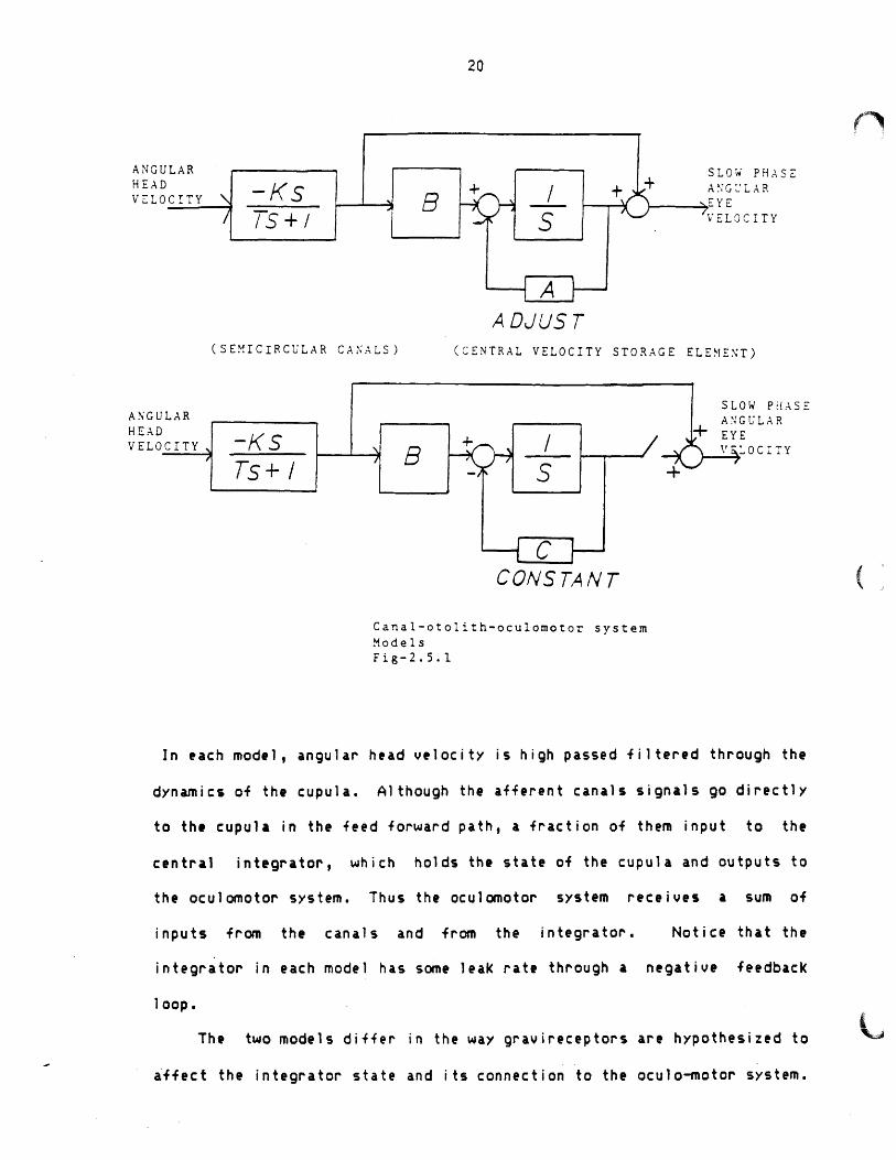
Figure 2.5.1 show two suggested block diagrams to model the
semicircular canal-gravireceptor-oculomotor system (Oman, personal
communication). They were based on the model of Raphan and Cohen, but
leave out other blocks relating to the optokinetic tracking system.
Page 21
20
ANGULAR SLOW PH SEHEAD + A;G :L A R
VELVCLOYIYE
ADJUST(SEMICIRCULAR CANALS) (CENTRAL VELOCITY STORAGE ELEMENT)
SLOW PHASEANGULAR A NGULARHEAD + EYEVELOCITY -S0 'OCIT
TS+l S +
CONSTANT
Canal-otolith-oculomotor systemModelsFig-2.5. 1
In each model, angular head velocity is high passed filtered through the
dynamics of the cupula. Although the afferent canals signals go directly
to the cupula in the feed forward path, a fraction of them input to the
central integrator, which holds the state of the cupula and outputs to
the oculomotor system. Thus the oculomotor system receives a sum of
inputs from the canals and from the integrator. Notice that the
integrator in each model has some leak rate through a negative feedback
loop.
The two models differ in the way gravireceptors are hypothesized to
a4fect the integrator state and its connection to the oculo-motor system.
Page 22
21
In the top model, gravireceptors change the leak rate of the central
integrator by adjusting the gain of the feedback element. In the bottom
model, gravireceptors gate the signal of the central integrator away from
the oculomotor system.
These models predict different time course rotational slow phase eye
velocity both when the head tilts forward and when the head is brought
upright again. The implications will be discussed later.
Page 23
Chapter 3
Experimental Procedure.
Vestibular experiments were conducted at the NASA Dryden Flight
Research Facility at Edwards Air Force Base, California by Oman and
colleagues. EOG signals were recorded in analog form on FM magnetic
tape. The data was digitized in the M.I.T. Man-Vehicle Lab by Eve
Riskin. She used a PDP-11 computer which was manufactured by the Digital
Equipment Corporation and an A/D program called SPARTA Lab Applications-
11 which was also a marketed by DEC. Most of the work for this thesis
comprised preparing and stripping the slow phase eye velocity from a raw
nystagmus signal and then analyzing the experimental data. The
experimental protocol proceed
Identical tests were
astronauts were tested prefli
and were tested postflight.
before the flight. The prefl
-121, -65, -43, -10 days
performed on the flight crew
and +4.
The same protocol was
subject sat upright in a chai
axis. Surface electrodes
record vertical and horizontal eye
movements were only of interest
blindfolded, but were told to keep
and mental arithmetic were used to
ed as follows:
(performed preflight and postflight. Six
ght. Four of those six flew on the mission
Subjects were tested on five separate days
ight tests were performed on days -151,
prior to launch. Post flight tests were
three times after landing on days +1, +2,
followed for each subject on
r which could rotate about
were placed on the skin besi
movements, although h
to this investigation.
eyes open during a test.
keep subjects alert.
each day. The
the vertical
de the eyes to
orizontal eye
Subjects were
Conversation
'L
Page 24
23
A subject with the head upright was given a step angular velocity of
120 degrees per second in the clockwise direction for 60 seconds. The
chair was then stopped within 1 second. Eye movements were analyzed for
45 seconds from the time the chair began to decelerate. These eye
movements are referred to as the post rotational vestibular ocular reflex
(PVOR). One minute aTr t - :-1 :na. stopped, the same procedure a=
repeated in the counterclockwise direction. This test will be referred
to as a "head up PVOR."
Next, one minute after the chair stopped rotating counterclockwise,
it was again brought up to speed in the clockwise direction to start
"tilt suppression" experiments. When the chair stopped, the operator
started counting on the secon
seconds, the subject ti-lted
did not bring it back up until
eye movements were analyzed
commanded to stop. One minute
repeated the counterclock
to as a "tilt suppression" or
Additional tests were
investigation. The EOG gain
head up PVOR test, before the
last tilt suppression test.
- To calibrate EOG gain,
and the operator zeroed the DC
voltage. It was necessary to
d: 0-1-2-3-4-"down"-6-7-8-9-"up". At 5
his head down approximately 90 degrees and
the operator counted to 10. As before,
for 45 seconds from the time the chair was
after the stop, the same procedure was
wise direction. This test will be referred
"head down PVOR."
then performed as part of a different
was calibrated immediately before the first
first tilt suppression test, and after the
a subject stared at a target directly ahead
component of the EOG amplifier output
determine how many millivolts were recorded
per angle of eye gaze. Keeping the head still, the subject then looked
at targets to the left and to the right which were strategically placed
Page 25
24
to require a 10 degree gaze angle. The surface electrodes measured a
vol tage proportional to a component of the corneo-retinal potential
across the eye globe and thus proportional to angular eye position.
The EOG gain was calculated with eyes open, but the magnitude of the
corneo-retinal potential changed as the eyes dark adapted when the
subject put on the blindfold. Therefore the EOG gain was calibrated
approximately every four minutes. EOG gain was interpolated between
calibrations for each vestibular test.
Page 26
25
Chapter 4
Data Processing
4.1 Overview of data processing
Five steps were required to prepare eye movement data recorded
during a vestibular test for analysis.
1) Angular eye position was recordaby Oman at Dryden as a raw EOG
signal.
2) The EOG signal was digitized at 100 Hz by Riskin at M.I.T.
3) A computer algorithm developed by Massoumnia at M.I.T. stripped
its best estimate of slow phase eye velocity from the EOG signal.
4) Corrections of slow phase velocity were made by hand by the
author with an interactive screen graphics program by DEC called SPARTA
when the algorithm failed to perform adequately.
5) The data was transferred to a second PDP-11 computer where slow
phase velocity signal was resampled to 4 Hz. Data was then transferred
to an Apple Ilc computer for statistical analysis using the program
STATSPLUS (Human System Dynamics, Inc). Data was plotted using a version
of DOTPLOT (CMI-Cascade, Inc) modified by Brian Rague.
Work for this thesis involved steps 3, 4 and 5.
4.2 Detection of slow phase movements
The top of Figure 4.2.1 shows a typical EOG nystagmus saw tooth
shaped signal that was recorded during this investigation.
Page 27
26
-1
1 ~ ~ j~41i.~ Lk)
I " U
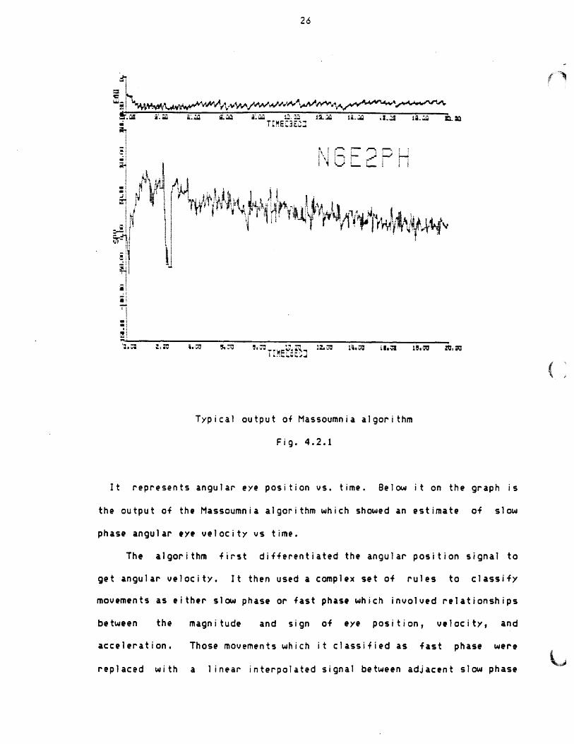
Typical output of Massoumnia algorithm
Fig. 4.2.1
It represents angular eye position vs. time. Below it on the graph is
the output of the Massoumnia algorithm which showed an estimate of slow
phase angular eye velocity vs time.
The algorithm first differentiated the angular position signal to
get angular velocity. It then used a complex set of rules to classify
movements as either slow phase or fast phase which involved relationships
between the magnitude and sign of eye position, veloc i ty, and
acceleration. Those movements which it classified as fast phase were
replaced with a linear interpolated signal between adjacent slow phase
Page 28
27
movements. To better understand how the Massoumnia algorithm worked,
observe Figure 4.2.2.
.IqL
i S.:j4 i
- 2 aJ LI
ii R Ji '21!i P::
j£ ' M~bI j 2j jif :_. . . ..H
H - * ~ .
W 3 61 6P6 ; 4V
. 441 f li W I I L
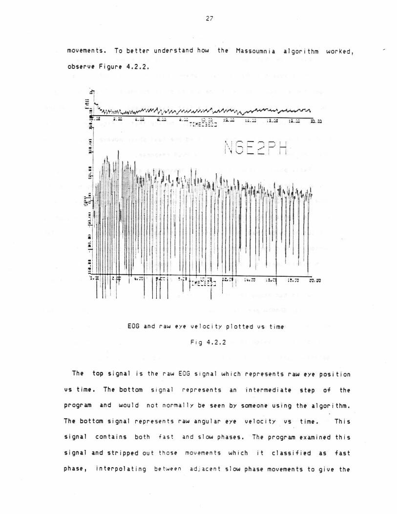
EOG and raw eye velocity plotted vs time
Fig 4.2.2
The top signal is the raw EOG signal which represents raw eye position
vs time. The bottom signal represents an intermediate step of the
program and would not normally be seen by someone using the algorithm.
The bottom signal represents raw angular eye velocity vs time. This
signal contains both fast and slow phases. The program examined this
signal and stripped out those movements which it classified as fast
phase, interpolating between adjacent slow phase movements to give the
.20
Page 29
28
estimated slow phase eye velocity signal that was shown in Figure 4.2.1.
It is possible that a fast phase movement can satisfy al
algorithm's requirements to be a slow phase movement. Thus the p
sometimes erroneously classified a fast phase movement as a slow
movement and did not strip it out. Notice that in Figure 4.2.1
program apparently only misclassified one fast phase movement as a
phase movement two seconds into the PVOR response.
Fast phase movements which the Massoumnia algorithm failed to
out were removed with an interactive screen graphics program
SPARTA on a PDP-11, both of which were sold by DEC. This program a
a file containing the slow phase velocity output from the Mass
subroutine to be read into a buffer which was displayed on a CRT.
I the
rogram
phase
the
sl ow
strip
cal led
11 owed
oumn i a
Two
could be positioned anywhere on discreet points
entiometers. Using appropriate commands, points of
the two buffers could be deleted and replaced wi
ch had endpoints on the cursors.
s, SPARTA provided a way to linearly interpolate
representing slow phase eye velocity over portions
se eye velocity which the program failed to delete.
of the signal
the signal
th a straight
between two
representing
Because the
deleted part of the signal was replaced with a straight line, the
interpolation made that part of the slow phase angular eye acceleration
appear constant in time.
As mentioned before, slow phase angular eye velocity in response to
a step head angular velocity is approximately a decaying exponentIal.
However, during the time up to one or two seconds in which fast phase
movements were stripped ou t wi th SPARTA, slow phase velocity was
approximately constant.
cursors
with pot
between
line whi
Thu
portions
fast pha
(
IL
Page 30
29
Figure 4.2.3 shows the same signal in Figure 4.2.1 after Sparta was
used to remove a a fast phase movement in the
slow phase velocity record profile.
I Z.
EOG and corrected slow phase velocity plotted vs time
Fig 4.2.3.
Cursors were positioned at the beginning and the end of the fast phase
movement at two seconds into the record. SPARTA deleted the data points
between the cursors and performed a linear interpolation between. After
records were processed with Sparta, they were resampled from 100 Hz to 4
Hz to give a signal resembling that in Figure 4.2.4
Page 31
30
IL :7 -dj . 14 .
Slow phase eye velocity sampled at 4 Hz.
Fig 4.2.4
4.3 Criteria for correcting mistakes of the algorithm
Fast phase movements not removed by the Massoumnia algorithm had to
be manually stripped out with SPARTA because data analysis would involve
averaging across files. Misclassified fast phase movements such as those
shown in Figure 4.2.2. would bias the average too low and greatly
increase the variance for the slow phase velocity for a particular point
in time. Missed saccades were manually stripped out with guidelines
which were consistently followed:
1) When slow phase velocity was high (greater than about 60 degrees
per second), the EOG signal contained high nystagmus beat frequency, low
amplitude eye movements. Analog filters in the recording
instrumentation, and digital filters in the algorithm to reduce high
frequency noise, rounded out the high frequency fast phase movements to
Page 32
31
make them appear as slow phase movements to the algorithm. Thus the
program passed these fast phase movements instead of interpolating over
them. In this case when the human eye could clearly separate fast phase
movements from slow phase movements in the EOG signal, but the algorithm
failed to do the same, the fast phase movements were manually removed.
As the experimental procedure will later describe, slow phase velocity
was highest at the beginning of the vestibular test. Thus, the algorithm
failed in this respect here the most.
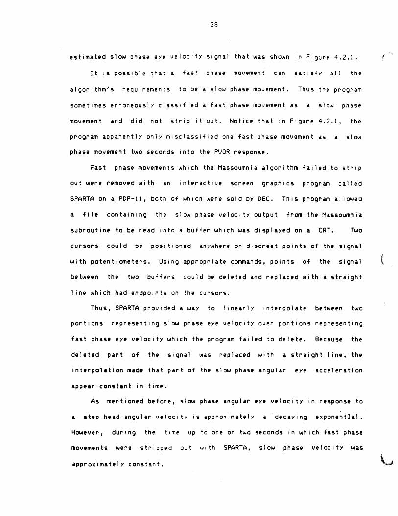
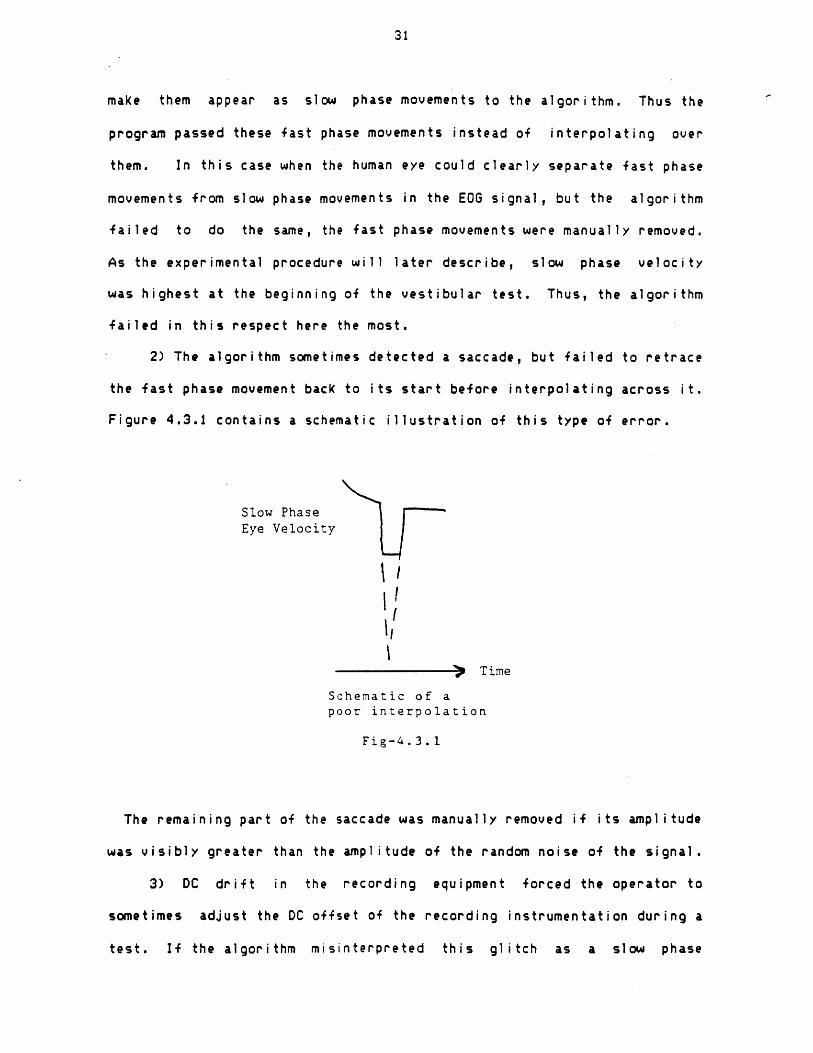
2) The algorithm sometimes detected a saccade, but failed to retrace
the fast phase movement back to its start before interpolating across it.
Figure 4.3.1 contains a schematic illustration of this type of error.
Slow PhaseEye Velocity
) Time
Schematic of apoor interpolation
Fig-4.3. 1
The remaining part of the saccade was manually removed if its amplitude
was visibly greater than the ampl itude of the random noise of the signal.
3) DC drift in the recording equipment forced the operator to
sometimes adjust the DC offset of the recording instrumentation during a
test. If the algorithm misinterpreted this glitch as a slow phase
Page 33
32
movement, i
4) If
time, the
test and wo
noise in
interactive
was evident
5) In
the veloci
Remember th
it upright
drop in the
instrumenta
t was manually removed.
the signal to noise ratio of an EOG signal was not constant in
algorithm sometimes completely failed in some sections of a
rked adequately in others. Up to two seconds of worthless
the velocity signal was manually interpolated out with the
screen graphics program if a clean slow phase velocity signal
on either side.
slow phase eye velocity profiles of tilt suppression tests,
t
a
t
y signal
t subject
again a
velocity
ion or
artifact may be that
to transiently roll
the component of t
electrodes near the
contributed. Brief t
often transiently droored at 5 and 10 seconds.
s tilted the head forward at 5 seconds and brought
t 10 seconds. It is not known whether this apparent
signal was due to an artifact of the recording
a true velocity transient. One possible technical
pitching the head forward and back caused the eyes
up and down in the head, which transiently changed
he corneo-retinal potential recorded by surface
temples. Electrode motion artifact may have also
ransients occurring at 5 at 10 seconds were removed.
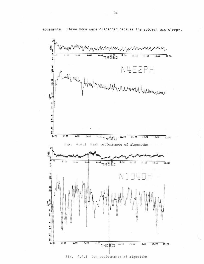
4.4 Criteria for discarding files
The performance of the program depended most importantly on the
signal to noise ratio of the EOG signal. Figure 4.4.1 shows one file for
which the program interpolated the slow phase velocity across almost all
saccades. The top signal is the raw EOG signal which represents angular
eye position vs time. The bottom signal represents the slow phase eye
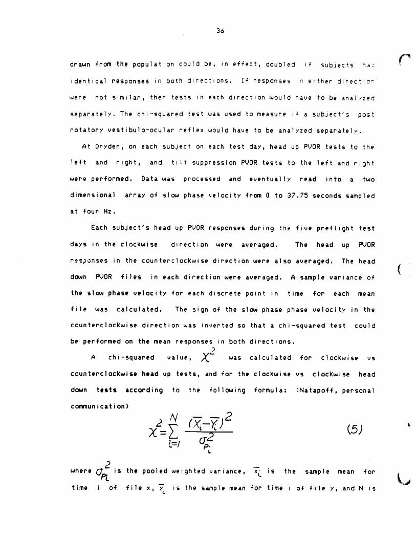
velocity vs time of that signal. Figure 4.4.2 shows one file in which
noise in the EOG signal cause the algorithm to fail frequently.
Page 34
33
The program correctly identified and stripped out approximately 50%
to 95. of all saccades depending largely on record noise level. This
performance varied greatly between subjects. Some subjects had a
consistently low corneo retinal potential and thus had a high signal to
noise ratio which caused the algorithm to fail. Researchers who plan to
use this program might consider choosing test subjects with a high
corneo-retinal to extract optimal performance form the Massoumnia
algorithm.
In this investigation, 145 EOG signals from separate vestibular
tests were input to the stripping program. 21 (13%) were not used for
data analysis. Although files were discarded from all subjects, profiles
of responses from subject 1 were discarded more than the others because
he had a consistently -low EGG gain. Files were discarded for the
following reasons.
1) A relatively noiseless EOG signal sometimes became extremely
noisy, suggesting that an electrode lost good contact with the skin.
2) An EGG signal had such a constantly high signal to noise ratio
that the algorithm completely failed to strip slow phase eye velocity.
3) The beginning of a velocity profile from a PVOR test showed no
eye movement at all. This indicated that the the beginning of the
profile was missed when data was transferred from FM tape to digital
media. Some profiles showed a low initial response, as opposed to no
initial response. It was believed that subjects with, a high initial
slow phase velocity for most PVOR tests who had virtually absent
responses to stopping the chair were likely sleepy during that portion of
the test. These files were discarded only if the response profile was
Three records were discarded that contained no eyemarkedly atyp ical .
Page 35
34
movements. Three more were discarded because the subject was sleepy.
AA* upfyA .A
V. W, V/ VW
W .!A. a. *~ ~
W4 AI~x 7. -Nq :'
it. :
'ia i
Fig. 4.4.1 High performance of algorithm
HqV.ij
5.
a'
'IJ
1 .5.I .~:Fj4~~
f~j hag'
If
I-~ ~ as- -M~
Fig. 4.4.2 Low performance of algorithm
I I
1 .96 w
a
- -9 --- ?4969 W16;i 1 7.19
Art,T !. wA
i
5:16 4W iITO S ZZg
Page 36
35
Chapter 5
Strategies For Analyzing The Data
5.1 Two statistical methods for analyzing PVOR data
Remember that the primary goal of this experiment was to
characterize the pre and post spaceflight head up and head down slow
phase eye velocity profiles of the post rotational vestibulo-ocular
reflex. A general method was needed to test if two PVOR responses were
statistically significantly different. The chi-squared test was used to
test if two mean responses were significantly different without fitting
those responses to a model. A method was also needed to test what fitted
model parameters, if any, made two PVOR responses different. A t-test was
used to test if the parameters of model fits were significantly
different.
Before proceeding with a discussion of the statistical analysis
performed for this project, it is necessary to outline the circumstances
in which the analysis was conducted. This investigation had to proceed
within a strict schedule, and unexpected problems with computer hardware
prevented the manipulation of much of the data which was required to
perform the most comprehensive statistical analysis. A preliminary
statistical analysis was performed with the intent of documenting
possible changes in PVOR head up and head down responses preflight and
postflight.
5.2 Combining cLockwise and counterclockwise responses
Because identical tests were performed on each subject in the
clockwise and counterclockwise directions, the number of sample responses
Page 37
36
drawn from the population could be, in effect, doubled if subjects ha:
identical responses in both directions. If responses in either direction
were not similar, then tests in each direction would have to be analyzed
separately. The chi-squared test was used to measure if a subject-s post
rotatory vestibulo-ocular reflex would have to be analyzed separately.
At Dryden, on each subject on each test day, head up PVOR tests to the
left and right, and tilt suppression PVOR tests to the left and right
were performed. Data was processed and eventually read into a two
dimensional array of slow phase velocity from 0 to 37.75 seconds sampled
at four Hz.
Each subject's head up PYOR responses during tne five preflight test
days in the clockwise direction were averaged. The head up PVOR
responses in the counterclockwise direction were also averaged. The head
down PVOR files in each direction were averaged. A sample variance of
the slow phase velocity for each discrete point in time for each mean
file was calculated. The sign of the slow phase phase velocity in the
counterclockwise direction was inverted so that a chi-squared test could
be performed on the mean responses in both directions.
A chi-squared value, was calculated for clockwise vs
counterclockwise head up tests, and for the clockwise vs clockwise head
down tests according to the following formula: (Natapoff, personal
communication)
2 Nx=Z
L=I
(X-Y)2
p.
(5)
2where is the pooled weighted variance, x, is the sample mean for
time i of file x, 7 is the sample mean for time i of file y, and N is
'I
Page 38
37
the number of points in time which are compared.
-YP L.-
where N is the number of records averaged into file x, N is the number of
records averaged into file y,e is the variance of, ),3 .is
the variance of . Chi-squared tables were obtained from Statistical2
Methods, by Snedecor and Cochran. If X = N, then the average squared
difference between the mean slow phase velocities foe each point in time
is equal to the pooled variance of that point in time, and thus the two
responses are significantly different. Chi-squared tables give 95%
confidence levels for the chi-squared value of each N. If n=100, then
the null hypothesis that two curves areI
ident ical is disproved with 95%
confidence when X is greater than 124. The slow phase velocity values
for 100 discrete points in time from 2 to 27 seconds were compared in the
chi-squared tests. The accuracy of the first two seconds was suspect
because of performance problems with the algorithm, as described earlier.
After 27 seconds, the slow phase velocity had decayed close to zero,
where factors such as alertness and adaptation became significant. Also,
chi-squared tables with N=100 were the largest located. The chi-squared
tests were performed on the records at 100 Hz before they were resampled
to 4 Hz.
The basis for the decision to average responses for a given subject
in a given direction across test days to obtain an estimate of his mean
response in that direction was that there was no trend, or learning
curve in a subject over the preflight testing period. To test this
assumption, chi-squared tests were performed on mean responses of the
Page 39
38
population on a given day. Chi-squared tests did not indicate that ine
difference of the mean responses of the population were significantIX-
different with 95% confidence between preflight testing days 1,3),
(1,5) and (3,5). However, this test only was useful for testing if
there was a preflight learning curve for the population. It said
nothing about the possibil ity of learning curves within individual
subjects. However, no trends were seen when the data was scrutinized by
eye for individuals and the analysis proceeded, noting the possibility
that individual trends may have affected the results of chi-squared tests
which compared right vs left rotations per subject.
The head up PVOR X values for subjects 1 ,2 ,3 ,4 ,5 and 6 obtained
by comparing mean preflight clockwise and counterclockwise directions
were 123, 86, 68, 86, 334, and 374. It is was not suspected that every
subject's PVOR responses would be similar in opposite directions, because
asymetries are commonly observed in humans. However, the chi-squared
test was used to examine which subjects had approximately similar
responses in either direction. The results of the chi-squared test
suggested that the difference between clockwise and counterclockwise
preflight head up PVOR responses was significant with 95. confidence for
subject 5 and 6. The X value for subject 1 was borderline in proving
that his responses were significantly different. Subject one had the
noisiest EGG signals and the Massoumnia algorithm performed least well
with him, so it is suspected that the algorithm exaggerated differences
between the responses, and it was judged that the clockwise and
counterclockwise head up PYOR tests could be averaged. Subjects 2 ,3 and
4 had similar preflight head up PVOR responses in either direction.
The preflight head down PJORX values for subjects 1 through 6
Page 40
39
were 124, 224, 114, 109, 303, and 401. Again, subjects 5 and 6 showed
significant differences between the clockwise and counterclockwise
directions and subject 1 was borderline. Subjects 3 and 4 had no
significant difference in either direction. The chi-squared test on
subject 2 indicated that the difference in the clockwise and
counterclockwise responses was significant . However, the two mean
responses appear very similar except for a few seconds where the signals
transiently digressed. This may be explained by the fact that few
numbers of test days were able to be averaged together for this subject.
Subject drowsiness or algorithm failure during only one PVOR test were
thought to have biased the mean responses in that direction. Because
subject 2 did not have significantly different head up PVOR responses, it
was decided that both his head up and head down PVOR files in either
direction could be averaged with some justification.
Only 2 of the 6 subjects (#3,#4) showed no significant difference in
preflight clockwise or counterclockwise head up or tilt suppression PVOR
tests. Because subjects 5 and 6 did not fly on the mission, and it was
observed that the their PVOR responses were not symmetric, their data was
not examined again. It was suspected that algorithm examined slight
differences in the directional responses of subjects 1 and 2. Thus the
above analysis concluded that clockwise and counterclockwise PVOR
responses could be averaged for individuals 1 ,2 ,3, 4, noting that it
was possible that minor asymetries could have been present to some
degree.
With the final goal to be able to average all preflight clockwise
and counterclockwise responses for each day for each subject, the
preceding chi squared analysis has suggested that:
Page 41
40
1) The mean PVOR responses for the sample population as a whole
changes little from day to day.
2) Clockwise and Counterclockwise PVOR responses were not materially
different for each of the first four subjects.
Before justifying the utility of such a global average, it was
first necessary to investigate the variance of the responses between
individuals. For a more accurate way of examining the source of this
variance, individual responses were fit to models. The results will be
presented in the next chapter.
(
Page 42
41
Chapter 6
Modeling Slow Phase Eye Velocity During A PVOR
In the most simple vestibulo-ocular model that does not account for
the central integrator or adaptation effects, canal afferent signals
drive slow phase eye velocity. The Steinhausen equation predicts that a
step head angular velocity elicits slow phase velocity which has a
profile resembling the response of a high pass filter with characteristic
time constant and gain. The Raphan and Cohen model predicts that a PVOR
response would better fit to a two time constant model. Oman and Young
(1969) have shown that adaptation effects require a PVOR response to be
fit to at least a three time constant model for more accuracy. However,
before attempting to fit data to a complicated model, it was decided that
the main features of nystagmus between 1 and 20 seconds could be
adequately described by a two parameter first order model with a time
constant and gain. Parameterizing head up PVOR responses with a gain and
apparent time constant provides a way of testing if two mean responses
differ mainly in the initial amplitude or in the rate of decay.
To provide a rough estimate of how well head up PVOR profiles would
fit to a one time constant model, the mean response of all preflight head
up PVOR responses was plotted + and - one standard error of the mean.
(It was noted that clockwise vs counterclockwise responses could be
different and that responses between subjects probably were not similar
in detail.) This signal, which is shown in Figure 6.1.1, approximately
looks like an exponential.
Page 43
42
PREFLIGHT AVERAGE PUOR +/- 1 STANDARD ERROR OF THE MEAN
7'
20
e 18 20 30
TIME (SEC)
Fig. 6.1.1 Global preflight head up PVOR profile
If it truly were a decaying exponential, the natural log of the slow
phase velocity plotted vs time would be a straight line. The intercept
would equal the negative inverse of the time constant and the y-intercept
would define some characteristic gain. Figure 6.1.2 shows a scatterplot
of the natural log of the sample population's head up slow phase velocity
vs time from I to 20 seconds.
I
0L.
U1
0-j
U
0
:3M
-j(n,
I I
Page 44
43
LN SPV = -. 078 TIME + 4.264.222 - .
3.047
a.
2.459
1 7 13 20TIME (SEC)
Fig. 6.1.2 Model fit of mean preflight head up PVOR
The line in the plot minimizes the sum of squares of the errors
between the line and the points. This plot suggests that the data can
be approximately parameterized to a one time constant model, at least for
twenty seconds of a PVOR. It was known that the one time constant model
for slow phase angular eye velocity would break down at some time during
a PVOR because of adaptation effects (probably in the peripheral neuron)
which create nystagmus in the opposite direction after 25 to 35 seconds.
Page 45
44
Oman (1969) suggested that the time constant for these adaptation effects
is about 80 seconds. Thus fitting the head up PV)OR time constant to a 1
time constant model for twenty seconds was somewhat justified.
i A
Page 46
45
Chapt
Resu
er 7
i ts
7.1 Mean PVOR Responses of Individuals
Chi-squared tests comparing mean responses of the
population for preflight test days 1, 3, and 5, did not prove
responses were significantly different at the 5% level. Thus
no obvious trend in the responses over time of the population.
possible that there were counterbalancing trends in individuals
4 subject
that mean
there was
It is
but this
is not likely because no I
individual responses with
suppression tests were aver
the four subjects to obtain
mean postflight tilt suppr
responses were fit to first
the slow phase velocity
recipro~ca o the slope then
ndividual trends were observed
the eye. Preflight head
aged across the five testing d
a mean preflight head up PVOR
ession PVOR response for each
order models by plotting the n
vs time from 1 to 20 seconds
renresented an apoarent time
when exanin
up and t
ays for each
response and
subject. Th
atural log
The negat
constant
the inverse natural log of the y-intercept divided by
velocity in angular degrees per second) represented
shows the results of individual subject model fits.
120 (the input step
a gain. Table 7.1.1
ing
ilt
of
a
ese
of
ve
and
Page 47
46
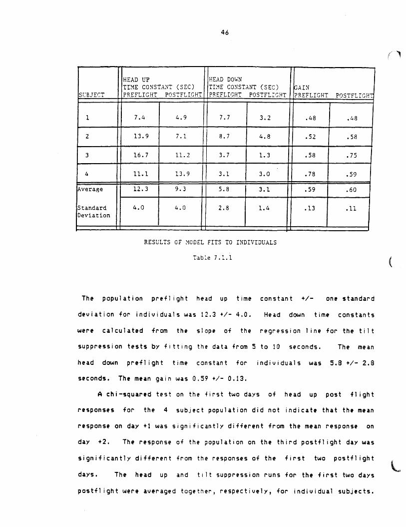
HEAD UP HEAD DOWNTIME CONSTANT (SEC) TIME CONSTANT (SEC) AIN
SUBJECT PREFLIGHT POSTFLIGHT PREFLIGHT POSTFLIGHT PREFLIGHT POSTFLIGH.
1 7.4 4.9 7.7 3.2 .48 .48
2 13.9 7.1 8.7 4.8 .52 .58
3 16.7 11.2 3.7 1.3 .58 .75
4 11.1 13.9 3.1 3.0 .78 .59
Average 12.3 9.3 5.8 3.1 59 .60
Standard 4.0 4.0 2.8 1.4 .13 .11Deviation
RESULTS OF MODEL FITS TO INDIVIDUALS
Table 7.1.1
The population preflight head up time
deviation for individua
were calculated from
suppression tests by fi
head down preflight
seconds. The mean gain
A chi-squared test
responses for the 4
response on day +1 was
day +2. The response
significantly different
days. The head up
ls was 12.3 +/- 4.0.
(/
constant +/- one standard
Head down time constants
the slope of the regression line
tt I ng
time
was
on t
subj
si gnI
of t
from
the data from 5 to 10 seconds.
constant for individuals was
0.59 +/- 0.13.
he first two days of head up
ect population did not indicate t
ficantly different from the mean
he population on the third postfl
the responses of the first two
for the tilt
The mean
5.8 +/- 2.8
post flight
hat the mean
response on
ight day was
postflight
and tilt suppression runs for the first two days
postflight were averaged together, respectively, for individual subjects.
Page 48
47
Post flight head up and head down time constants were calculated from
model fits. The mean postflight head up time constant for individuals
+/- 1 standard deviation was 9.3 +/- 4.0 seconds. The mean postflight
head down time constant for individuals +/- one standard deviation was
3.1 +./- 1.4 seconds. The post flight gain was 0.60 +/- 0.11 These
results are shown next to the preflight results in Table 7.1.1. Pre and
post fl ight head up and head down, or nystagmus dumping, time constants
are shown for individual subjects in bar graph form in Figure 7.1.2.
Page 49
- ~ --1 - - - -- ----- -
48
Preflight and Postflight Headuo PVOR Time Constants
Preflight
Postflight
l8secs.
16secs.
l4secs.
12secs.
IOsecs.
8secs.
6secs.
4secs.
2secs.
Osecs.2 3 4
Subject
Preflight and Postflight Dumping PVOR Time Constants
[Prefight
. Postflight
+4- -4
1 2 3 4Subject
Fig 7.1.2
TImC
C0nSt
nt
+4
1
Tim
nn
t
nt
9secs.
8secs.
7secs.
6secs.
5secs.
4secs.
3secs.
2secs.
Isecs.
Osecs.
Page 50
49
Notice that the mean head up Qostflight time constant was less than the
mean head up p-eflight time constant for subjects 1, 2, and 3. Subject 4
had a slightly higher mean postflight head up time constant than
preflight. The mean postflight head down time constant appeared less
than the mean preflight head down time constant for subject 1, 2, and 3.
Subject 4's head down response appeared unchanged preflight to post
flight. There appeared to be no significant trend in the PVOR gain
preflight to postflight.
The preceding analysis across days for each subject has given an
estimate of the mean preflight and post flight head up and head down time
constants and gains for the sample population. We are interested in
learning if living for 10 days in weightlessness caused the vestibulo-
ocular system to adapt in ways that ca
to quantify the possible difference b
responses, independent sample t-tests
parameters of the apparent head up and
PVOR gain. However, neither indep
disproved the null hypothesis with 95.
difference pre and post flight in th
constant, head down time constant or
responses between subjects was t
significant conclusions to be drawn abo
post flight responses of the population
A chi-squared analysis comparing
responses for individual subjects
subject 2
However,
and 4 were significantly di
the mean head up time constant
n be measured. As a first
etween preflight and po
were performed on the subji
head down time constants
endent or dependent sample
confidence that there
e sample population's head
gain. The variance
oo large for any stati
ut the changes in the mean
with a t-test analysis.
pre and post flight
indicated that the resp
attempt
itfl ight
ect mean
and the
t-tests
was no
up time
in the
stically
pre and
head
onses
fferent pre and post flight.
of subject 2 was less postflight
up
of
Page 51
50
than preflight. The mean head up time constant for subject 4 was greater
postflight than preflight. A
flight head down responses
responses for each subject
postflight. However, this re
The chi-squared test was
which might have changed pref
slow phase velocity at 5 to
the gain of the response from
chi-squared analysis comparing pre and post
for individual subjects indicated that
were significantly different preflight and
sult must be cautiously interpreted.
sensitive to any parameters of the response
light to postflight. The magnitude of the
10 seconds depends on the time constant and
1 to 5 seconds. Thus although the chi-
squared test indicated that the preflight and postflight head down time
constants for each subject could not be superimposed on the same graph,
the chi-squared test could not relate if this was due to a change in the
gain, the head up time constant, or the head down time constant.
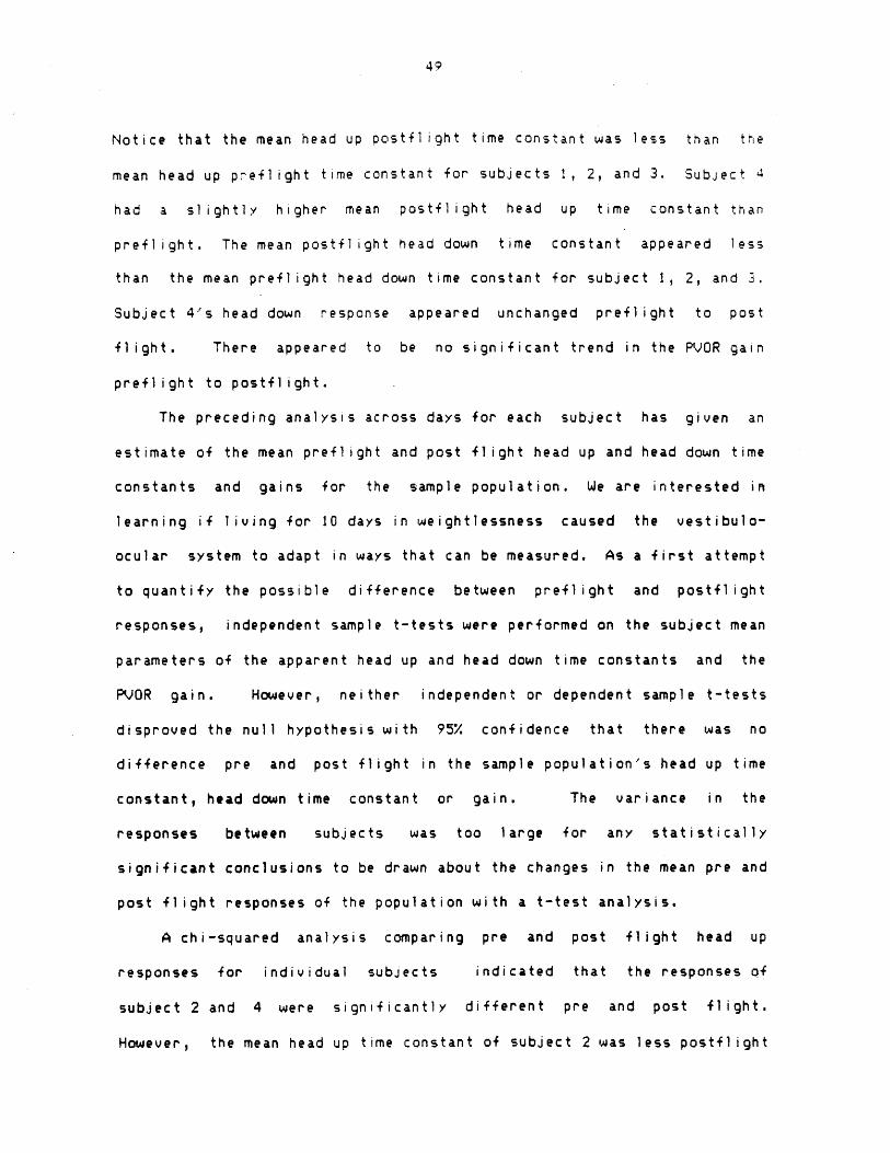
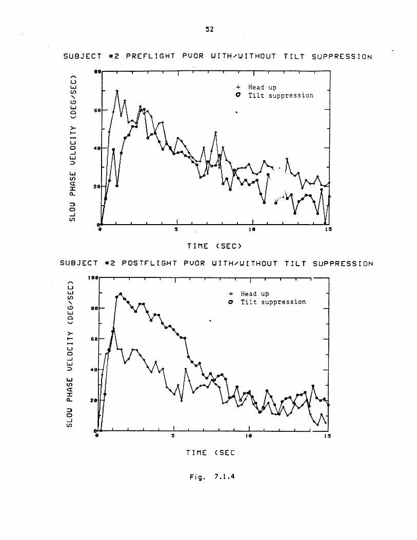
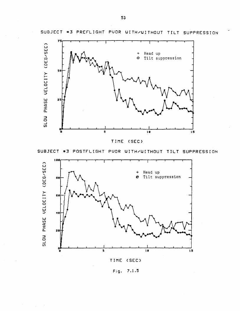
Figures 7.1.3-7.16 show the mean preflight and postflight head up
and tilt suppression PVOR responses for individuals. The plots show
post rotatory slow phase eye velocity vs time.
( 01
Page 52
51
SUBJECT #1 PREFLIGHT PUOR ULTH/UITHOUT TILT SUPPRESSION
LoLi
(.J
LD0-jLi
Li(I,
0-J(I,
5 is 15
TIME (SEC)
SUBJECT
97LLLi
.DL-
-)0-jLiJ
Li(1)<r
a-
0-J(I)
77
57
37
17
-3
#1 POSTFLIGHT PVOR UITH/U[THOUT TILT
-23
5 is
SUPPRESSION
15
TIME (SEC)
Fig. 7.1.3
I I -- T II I I I
+ Head upo Tilt suppression
30
18
is
-I I I I I I I I
uppressiono Tilt s+ Head up
Is I
I I I I
I I
58
Page 53
52
SUBJECT #2 PREFLIGHT PUOR UrTH/UITHOUT TELT SUPPRESSION
+ Head upo Tilt suppression
48-
28
is0 15
TIME (SEC)
SUBJECT *2 POSTFLEGHT PVOR UITH/U[THOUT TILT SUPPRESSION
I I I
+ Head up
O Tilt suppression
i8
TIME (SEC
Fig. 7.1.4
V)
Wi
U
LD
a-
L)0
se
s6
I I I I
L)J
e-%
LiJ
U
CD
<IL)
0
-
Li
Li
cr
:30-j
48
28
5
by"d
Page 54
53
SUBJECT #3 PREFLIGHT PUOR UETH/UITHOUT TILT SUPPRESSION
50
U
CDLi
0-JLiJ
LiJ
0-JLo)
5 1s 15
TIME (SEC)
SUBJECT #3 POSTFLIGHT PVOR UITH/U[THOUT TILT SUPPRESSION
5
TIME (SEC)
F i g. 7.1.5
+ Head up0 Tilt suppression
- -25
~m. * , * I * * * . I
Be+ Head upo Tilt suppression -
Lo
U
0-j
<ra_
0
Uj
60
48
20
-s 1 15
-ff -K
1
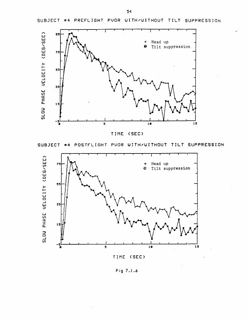
Page 55
SUBJECT #4 PREFLIGHT PVOR UrTH/UITHOUT TILT SUPPRESSION
5 Is 15
TIME (SEC)
SUBJECT #4 POSTFLrGHT PVOR UITH/UTHOUT TILT SUPPRESSION
5
TIME (SEC)
Fig 7.1.6
95
75
55
U
Lij
0-
0
Li
LijLo
0-jUf)
+ Head upTilt suppression
35
I I I I I
+ Head up
O Tilt suppression
U
Li
L-
0-jLi1
Lij(f)
:30
75
55
35
15
I I Ii 1 5
II I I I I i
Page 56
Chi-squared tests were performed on these plots to discover !4
individual subjects exhibited tilt suppression of nystagmus Pre or
postflight. In the tilt suppression tests, the head was tilted down from
5 to 10 seconds after the rotating chair stopped. Head up and head down
responses from 5 to 10 seconds were compared with the chi-squared test,
It indicated that preflight head up and tilt suppression responses from 5
to 10 seconds were significantly different with 95 % confidence for
subjects 3 and 4. Postflight head up and tilt suppression responses from
5 to 10 seconds were significantly different for subject 2, 3, and 4,
indicating that tilt suppression continued to occur postflight.
7.2 Mean Daily Responses of the Population
Regardless if the population preflight head up PVOR responses are
calculated by averaging responses across subjects for each test day or by
averaging across test days for each subject, the values of the means
should be the same, though the variances and hence regression model fits
could be different. Although each subjects PVOR response may vary
greatly from each other, each subject may have consistent responses for
each test day. It was hypothesized that the great variance in the
responses between subjects made it hard to prove with a t-test analysis
that the mean responses of the population were significantly different
preflight and postflight. Thus another view of the mean preflight and
postflight head up and tilt suppression responses was obtained by first
averaging the responses of the 4 subjects on each of the five preflight
testing days and each of the first two postflight testing days.
For each testing day, models were fit to the mean head up and head
down responses averaged across the four subjects. Results of these model
Page 57
fits are shown in Table 7.2.1.
DAYS PRELAUNCHOR HEAD UP HEAD DOWN
POSTLANDING TIME CONSTANT (SEC) TIN!E CONSTANT (SEcr) GAIN
-151 11.0 3.5 .65
-121 12.7 3.5 .76
-65 19.6 2.5 .44
-43 11.0 4.1 .56
-10 12.2 2.2 .52
+1 9.1 2.3 .62
+2 9.5 4.4 .58
+4 12.3 3.5 .59
Daily model fits
Fig-7.2.1
Figure 7.2.2 shows in bar graph form the mean head up time constants
for the population on each test day.
Page 58
57
Headup PVOR Time Constants per Day AveragedAcross Subjects
-121 . -65 -43 -10Day
+1 +2 +4
Fig 7.2.2 Results
head up
of model fits to preflight
PVOR responses
Notice that thii Toan head up time constant of the population on the third
test day (65 days prior to launch) is almost twice as large as the mean
time constant of the population for the other two days. Although the
variance of the daily mean preflight head up time constants is 13.0, the
variance excluding the third test day is 0.9. This makes the accuracy of
data from that day suspect, although no obvious explanation for the
consistently longer responses could be found. Ignoring test day #3, the
average of the daily mean preflight head up PVOR time constants +1- one
standard deviation was 11.7 +/- 0.9 seconds. The postflight head up
average for days +1 and +2 was 9.3 +/- 0.3 seconds. An independent
T
m
C0nStant
19secs.
17secs.
15secs.
13secs.
11secs.
9secs.
7secs.
5secs.-151
-- 4I I I I - -..- +--
Page 59
58
sample t-test indicated that the difference of the mean preflight and
postflight head up PVOR responses was significant with 95% confidence.
The mean head down PVOR time constant on test day #3 did not look
suspicious, although the head up time constant appeared different. The
average of the five preflight daily mean head down time constants was 3.2
+/- 0.8 seconds. The mean postflight head down average for days +1 and
+2 was 3.4 +/- 1.5 seconds. A t-test -dicated that the difference in
these means was not statistically significant.
7.3 GLobal Response of the Population
Up to now, we have averaged responses across days for each subject
and have averaged responses across subjects for each day. Although the
means are similar in each case, there is somewhat more variability
between subjects than between days, especially if preflight day #3 is
ignored. A third estimate of the mean response parameters of the
population was obtained by averaging responses across days and across
subjects. In other words, a mean response was calculated by averaging
all tests of each subject on each day. Figure 7.3.1 shows mean
prefl ight head up and t i suppression responses from 0 to 15 seconds on
the same plot.
Page 60
59
PREFLEGHT PUOR UITH/UJTHOUT TILT SUPPRESSrON
5 18 15
TIME (SEC)
Fig. 7.3.1
The curves overlap from 0 to 5 seconds. However,
decayed more rapidly for the population when the head
seconds, consistent with Benson and Bodin's finding.
upright at 10 seconds, the rate of decay decreased.
the same data plotted on semi-in axes.
slow phase velocity
tilted forward at 5
When the head came
Figure 7.3.2 shows
6
4
LO)NLJLiU)
CDLjLi
LiU)<rI
:
CD-iU)
- I I' I ' ' j '
+ Head up
o Tilt suppression
0-[
, i m I I I I I I I : : ,
2
-eI
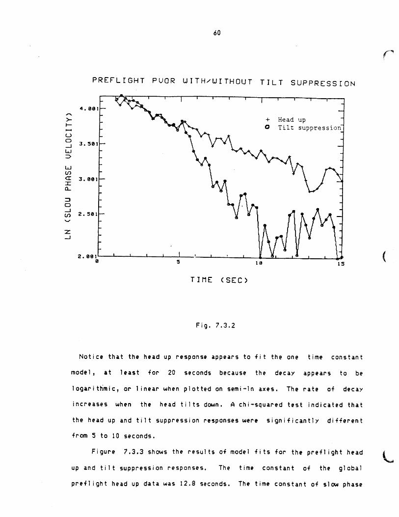
Page 61
60
PREFLEGHT PUOR UITH/UITHOUT TILT SUPPRESSLON
4. 881-
+ Head up0 Tilt suppression
U C)3. 501 -
U
C,)<r 3.881-
C-.
n 2.501-
2.881 ' ' ' '(
8 5 18 15
TIME (SEC)
Fig. 7.3.2
Notice that the head up response appears to fit the one time constant
model, at least for 20 seconds because the decay appears to be
logarithmic, or linear when plotted on semi-in axes. The rate of decay
increases when the head tilts down. A chi-squared test indicated that
the head up and tilt suppression responses were significantly differen t
from 5 to 10 seconds.
Figure 7.3.3 shows the results of model fits for the preflight head
up and tilt suppression responses. The time constant of the global
preflight head up data was 12.8 seconds. The time constant of slow phase
Page 62
61
velocity when the head was down from 5 to 10 seconds was 3.6 seconds.
The global preflight gain was 0.59.
SFU = +- . @7:3 TIME 4.2~LN
0U* U
S a
, a. .* U a
U Ol
U
a
a
- I I I
1 7 (He up)TIME (SEC)
LH NY P -. 725 TIME +.13 I
TIME10.000(Head down)
Fig. 7.3.3 MIodel fits for preflight PVOR tests
4. 222
C .- 4-3. 47
3. 22
CL
.2.642
001 U
078 T IME 4.-2 tn
Page 63
62
Fig. 7.3.3. Model fits of global preflight head up and tilt suppression
tests.
Figure 7.3.4 shows the the mean postflight head
suppression responses obtained by averaging responses
subjects for the first two days of postflight testing.
up
of
and t il t
the four
POSTFLIGHT PVOR UJTH/UITHOUT
8
so
40
28
0
TILT SUPPRESSION
1 15
TIME (SEC)
Fig 7.3.4
A chi-squared test on the head up and head down responses indi
they were significantly different with 95% confidence. Notice
tilt suppression does not appear as dramatic postflight
cated
that
as it
that
the
did
LONCDLi
CD
-JLi
Li
:3
-JU-)
+ Head upO Tilt suppression
- -I ~ _ -
(
[a
Page 64
63
preflight (Figure 7.3.2.). Model fits of the postflight head up and
head down responses, which are shown
4 . 2--3 1
CLU:)
f2 435
1.504
-
~2.433
1.871
C.
in Figures 7.3.5 may explain
177 13 2TI ME (SEC)
LN (SP = -. 2t5 TIME + 5.01
LAI
.000 6.667TIME
8.333(SEC)
10.000
Model fits for postflight global
this.
LH FP = -. 1C5 TIME + 4.27
% a 0 an
-0 C3 3n.
rU
Fig 7.3.5. head up and tilt suppression
Page 65
The global postfl ight head up PVOR time constant was 9.5 seconds. Tre
head down time constant was 3.8 seconds. The gain was 0.59. Thus the
tilt suppression may appear more dramatic preflight than post fight f:r
the global averaged responses because the postflight head up slow phase
eye veloci ty decayed faster than the preflight head up veloci ty, .wnicn
had an apparent time constant of 12.8 +/- seconds. By the time the head
tilted forward post flight, the slow phase angular eye velocity had
already decayed a good deal. The global model fits did not suggest that
either the head down time constant or the gain changed preflight to post
flight.
Figure 7.3.6 shows global pre and post flight head up PYOR
responses in linear-linear and log-linear form. A chi-squared analysis
of the global preflight vs postflight head up data showed no significan"
difference between 0 and 6 seconds, but a significant difference from o
to 20 seconds (It=111 for N=56). Since the first order model analysis
did not show statistical significance unless data from test day three was
omitted, it is not possible to conclusively interpret these findings.
Page 66
PREFLIGHT65
AND POSTFLIGHT HEAD UP PUOR
0L-LU
N
Lo
C-)
-j
Cr,
C)
-j(n,
18
PREFLIGHT AND POSTFLIGHT
19 15
HEAD UP PVOR
20 25
Fig. 7.3.6
TIME (SEC)
Sample population pre and post flight head up responses.
Notice that the responses begin to diverge at about seven seconds.
7
4.6931
20 40
PREFLIGHT
POSTFLIGHT
-jLi
Li 2.Cl)'I
:3
CD)
zIJ
. 69
6931 -
J ~.
30
5
55
35-PREFLIGHT
15POSTFLIGHT
a 30
Page 67
Howeter, Goldberg and Fernandez (1971) have shown "-i, '- 4ime constant
of afferent signals from the monkey semicircular canals is approximate',
5 to 6 seconds. If human responses are similar, and PVOR is sustainec n,.
te Raphan/Cohen central velocitY storage device, this analysis suggests
that although weightlessness does not affect the dynamics o4 the
semicircular canals, it makes the velocity storage integrator more leak-..
Thus the pre and post flight head up PVOR responses are similar to 6
seconds, during the time epoch where eye velocity is driven mainly by the
canals. After seven seconds, perhaps the afferent canal activity has
largely decayea, and slow phase eye velocity is driven by the central
integrator, which has become more leaky postflight.
Page 68
67
Chapter 8
Discussion
There were five major conclusions from this investigation of the
mean vestibulo-ocular responses of the sample population to a step
angular head velocity.
1) The mean preflight head up PVOR profile was statistical I
significantly different between 5 and 10 seconds from the mean preflight
head down profile for the sample population. Slow phase eye velocity was
suppressed when the head tilted down. These finding confirm those of
Benson and Bodin and others.
2) The mean postflight head up PVOR profile was statistically
significantly different between 5 and 10 seconds from the mean postflight
velocity profile for the first two days postflight for the sample
population. Slow phase eye velocity was suppressed when the head tilted
down.
3) Mean head up PVOR profiles were statistically significantly
different preflight vs the first two days postflight during the period
between 6 and 20 seconds after the chair stopped.
4) The preflight head down PVOR time constant was not statistically
significantly different from than the mean postflight head down time
constant for the sample population.
5) The preflight PVOR gain was not statistically significantly
different from the postfl ight PVOR gain.
The evidence of preflight tilt suppression is consistent with a
theory that the oculomotor system is driven partly by a gravity sensitive
central velocity storage element. If the head tilts forward 90 degrees
Page 69
08
when the afferent nerves from the horizontal semicircular canals are
signaling rotation in their plane, the slow phase eye velocity 4alls more
quickly than when the head remains upright. Thus the otol itn :rgans
might either open the pathway from the central velocity storage element
to the oculomotor system, as shown in the bottom of Figure 2.5.1 cr they
might greatly increase the leak rate of the integrator element, as shown
in the top of Figure 2.5.1. Afferent canal signals instead of afferent
central integrator signals become the dominant stimulus to the oculomotor
system when the head tilts.
If head tilt five seconds into a PVOR induced the otoliths to open
the circuit between the velocity storage element and the oculomotor
system, then slow phase eye velocity should instantaneously drop because
eye movement would only be driven by the canals which have a very short
time constant. The time constant of the slow phase velocity during head
tilt would equal the physical time constant of the cupula-endolymph
system, ignoring nonlinearities and adaptation affects. When the head
was brought back upright, otoliths signals would complete the circuit
between the central velocity storage element and the oculomotor system
and eye velocity should instantaneously rise to the level it would have
been at the time if the head was never tilted.
If head tilt five seconds into a PVOR induced the otoliths not to
open the circuit between the velocity storage element and the oculomotor
system, but to instead greatly increase the leak rate of the central
integrator, different eye movement dynamics would be observed. Slow
phase eye velocity would not instantaneously drop to the canal's estimate
of head velocity. It would decrease with a much shorter time constant
which was a function of the increased leak rate of the central
I
Page 70
integrator.
The most powerful way to test which theory best models
physiological system is to observe slow phase eye velocity when the iea
is brought back upright during a POR tilt suppression test, I the
otoliths open and close the circuit when the head tilts, eye veloc tv
should instantaneously rise when the head is bought upright again aro
resume the head up decay profile. If instead the otoli ths change the
leak rate of the velocity integrator, eye velocity will remain at the
same level when the head is brought upright because the integrator will
have discharged during the tilt. However, both models predict the head
up time constants before the head tilt and after the head is brought
upright to be the same.
Signals recorded from individual subjects were too noisy to
indicate conclusively if slow phase velocity rose when the head was
brought up in a tilt suppression test. Subject 3 may have demonstrated
that his preflight eye velocity increased after his head was brought
upright in a tilt suppression test. However,- it clearly did not climb up
the level of the control head up response. This data was shown in Figure
7.1.5.
Because tilt suppression of nystagmus was observed both preflight
and postflight and the preflight head down time constant was not
significantly different from the postflight head down time constant,
there was no evidence that the brain ignored signals from the otolitis
after ten days in weightlessness. It is possible that any adaptation
effects disappeared immediately after landing because the 1-g cues were
overwhelmingly strong after spending ten days in weightlessness. If no
tilt suppression occurred while in weightlessness, this would support
Page 71
model which give the otoliths the abilii
central velocity storage element as
signal measure head tilt.
An somewhat unexpected result of th
postflight head up PVOR response profile
the preflight head up PVOR profile start
rotating chair was stopped. There
weightlessness causes a change in t
semicircular canals within a week. The
from I to 20 seconds, derived from a one
the result of an adaptation process wi
ty to alter signal paths of t ne
they used the grav i ty -eC t:r
is investigation was to +inC tat
was significantly different rom
ing at seven seconds after the
is no evidence to indicate i
he physical structure of trOe
shortened apparent time constant
time constant model fit, may be
thin the central velocity storage
element or even within higher level brain
learns to pay less attention, in general
more attention to visual clues to drive
element.
functions in
, to the vest
the central
wh i c h
ibular
ve 1 oc
the brain
system, and
ity storage
Page 72
Appendix I
Suggestions For Other Experiments
1) In the tilt suppression experiments of this investigation, the
head was tilted forward five seconds after the chair was stopped anc
brought upright ten seconds after the rotating chair was stopped. B the
time the head was brought upright, slow phase eye velocity had aecreased
to the level where the signal to noise ratio was a problem for analysis..
Thus it was difficult to observe how the slow phase velocity changed when
the head was brought back upright. To test if the otoliths open tne
pathway from the central velocity integrator to the eyes or if the
otoliths increase the leak rate of the central velocity integrator, the
following protocol
The per rotat
tilt forward one
seconds after the
central velocity
should be signific
seconds of post
climbs when the he
theory that the
significantly to c
seconds after the
2) The basi
constant would be
is suggested:
ory procedure is unchanged. However, the head should
second after the chair stops and return upright five
chair stops. Assuming the canals can charge the
integrator in one second, the slow phase velocity
antly greater than the noise level after only five
rotatory response regardless of whether the velocity
ad returns upright. This protocol would also test the
central velocity storage element does not contribute
rive slow phase eye velocity until approximately seven
rotating chair stops.
s of the hypothesis that the preflight head down time
different than the postflight head down time constant,
after seven seconds from
interesting results of other
suspected that the brain
the stop of the rotating chair, was based on
sensory adaptation experiments. It was
would learn to interpret differently signals
Page 73
72
from the gravity sensing otol iths differently after a week in space.
is possible that after landing, the strong 1-g gravity cues immediatelv
made the brain respect otoli th signals again if it learned to ignore them
in weightlessness. If tilt suppression tests were performed immediately
after returning from orbit and they indicated that the postflight ead
down time constant was significantly different from the preflignt head
down time constant, this would be solid evidence of an adaptation process
which occurred in space. However, if no significant difference between
pre and post flight head down time constants was observed, then no
conclusions could be made about adaptation because whether or not in
space the brain learns to ignore signals from the otoliths which output
their best estimate of the gravity vector, the strong 1-g cues
immediately after returning to earth could quickly swamp evidence of a
slow adaptation to weightlessness.
3) Further analysis of the existing Slacelab 1 data is possible.
Second order Raphan-Cohen models should be fit to individual runs, and
then a two way analysis of variance performed.
Page 74
73
Appendix II
Listings of programs that resample, plot, and perform simple statistics
on files of slow phase velocity
The following programs can be found in the directory DPQ:[302,10J on
the DEC RSX system in the Man-Vehicle Lab.
SR
This program resamples 38.4 seconds of a slow phase velocity signal
from 100 Hz to 4 Hz so that it can be read by graphing and statistical
programs. The program first asks for the name of the file to be
resampled. This file must have 256 words per record. The program then
asks if the sign of the velocity should be inverted. It outputs time and
the resampled signal to a formatted sequential file with the same name as
the input file except that the first letter has been replaced by an "S".
FRAPH
Fraph must be run on a graphics terminal. It plots a raw EOG signal
and the corresponding 100 Hz slow phase velocity signal beneath it for 20
seconds. The program scales the EOG signal, but does not scale the
velocity signal when plotting. Both position and velocity files must be
sequential files. The position file must have extension (.EOG). THe
velocity file must have extension (.SPV).
SRAPH
This program must be run on a graphics terminal. It plots a slow
Page 75
74
phase velocity signal which has been sampled at 4 Hz vs tme for 20
seconds. The program reads formatted sequential files in which the time
and slow ;hase velocity is contained in each record.
PRO
This program finds the average, variance, standard deviation, and
sample error of the mean of points in time from 0 to 37.75 seconds of
sequential formatted slow phase eye velocity files sampled at 4 Hz. The
program asks for the number of files to be averaged, and the name of the
file to which it will write the formatted results sequentially. Each
record in the output file contains the time, average, variance, standard
deviation, standard error of the mean 'sem), ave + (sem), and ave -
(sem).
COMP
This program finds a chi-squared value relating the similarity of
two mean velocity profiles sampled at 4 Hz using a pooled variance
technique. The user inputs the names of the two files to be compared,
the number of files averaged into each mean file, and the desired time
interval for comparison. The program then outputs the number of points,
N, which were compared and the corresponding chi-squared value. The user
must then look up confidence intervals in chi-squared tables.
SEE
This program scrolls sequential files on the screen. It is designed
specifically to type time or slow phase velocity from files that contain
these parameters in the first to words of each record. There is a 6
Page 76
75
second delay after the user hits return to execute the program. After
all the data has scrolled, the user must hit the return key to exit tre
program.
Page 77
PDP-11 FORTRAN-77 V4.0-3 20:37:25 13-May-86 Page 1SR.FTN;16 /F77/TR:BLOCKS/WR
C ****** SR ******C THIS PROGRAM RESAMPLES A 38.4 SECOND DURATIONC 100 HZ SIGNAL TO 4HZ AND CHANGES THE SIGN OF THE VALUES,C IF DESIRED
0001 REAL Y(4000),RESAM(180),T0002 CHARACTER*10 TESTTEST20003 INTEGER BUF(256),S,C,J,K,LZEROFLIP
C READ IN FILE TO BE RESAMPLED
0004 2 TYPE*, ' ENTER FILE NAME'0005 READ(5,3), TEST0006 3 FORMAT(A10)0007 TEST2=TEST0008 TEST2(1:1)='S'0009 TYPE*, ' FILE READ IS...', TEST0010 TYPE*, ' FILE OPENED IS...', TEST20011 5 TYPE*, ' DO YOU WANT FILE INVERTED? (Y=1,N=0)'0012 READ(5,7), FLIP0013 7 FORMAT(Il)0014 90 FORMAT(Il)0015 95 FORMAT(F6.2,F6.1)0016 TYPE*, FLIP0017 IF(FLIP .EQ. 1)THEN0018 S=-1C ELSEIF(FLIP .EQ. 0)THENc J S=10021 ELSE0022 GOTO 50023 ENDIF0024 CALL ASSIGN(1,TEST,10)0025 DEFINE FILE 1(0,256,U,NREC)0026 OPEN(UNIT=2, FILE=TEST2,FORM='FORMATTED',
+ ACCESS='SEQUENTIAL',STATUS='NEW')0027 C=00028 DO 10 J=1,150029 READ(1'J)BUF0030 DO 20 K=1,2560031 C=C+l0032 Y(C)=BUF(K)*S0033 20 CONTINUE0034 10 CONTINUE0035 CLOSE(l)
C RESAMPLE FILE TO 4 HZ
0036 C=00037 ZERO=O0038 DO 15 M=1,1520039 WRITE(2,90), ZERO0'10 15 CONTINUEC . CLOSE(2)004*2 Y(1)=0.00043 OPEN(UNIT=2,NAME=TEST2,FORM='FORMATTED',ACCESS='SEQUENTIAL'
+ ,STATUS='OLD')
Page 78
77PDP-11 FORTRAN-77 V4.0-3 20:37:25SR.FTN;16 /F77/TR:BLOCKS/WR
13-May-86
DO 30 L=1,3800,25C=C+1T=L/100. -. 01RESAM(C)=Y (L)WRITE(2,95) TRESAM(C)
CONTINUECLOSE(2)CLOSE(l)GOTO 2END
0C .100460047004800490050005100520053
30
Page 2
I
Page 79
PDP-11 FORTRAN-77 V4.0-3SR.FTN;16
73'20:37:25
/F77/TR: BLOCKS/WR13-May-86
P- 'RAM SECTIONS
Number Name
1234
$CODEl$PDATA$IDATA$VARS
Size
001214000304000010041572
326984
8637
Attributes
RW,I,CONLCLRW, D, CON, LCLRW, D, CON, LCLRW, D, CON, LCL
VARIABLES
Name Type
CMTEST2
ARRAYS
1*21*2CHR
Address
4-0415524-0415704-040536
Name Type
FLIPNRECZERO
Address
1*2 4-0415641*2 4-0415661*2 4-041562
Name Type Address
JS
1*2 4-0415541*2 4-041550
Name Type Address
4-0405504-0372004-000000
Size
001000001320037200
Dimensions
256360
8000
(256)(180)(4000)
Label Address Label
1-000020**
Address Label
3'20
2-000000**
Address Label Address Label
530
1-000256**
FUNCTIONS AND SUBROUTINES REFERENCED
ASSIGN CLOS$ OPEN$
Total Space Allocated = 043322 9065
Page 3
Name
KT
1*2R*4R*4
BUFRESAMy
LABELS
215
Ad
7'90'
Page 80
PDP-11 FORTRAN-77 V4.0-3 20:50:23 13-May-86 Page 1FRAPH.FTN;4 /F77/TR:BLOCKS/WR
C ****** FRAPH ******C THIS PROGRAM USES THE VERSAPLOT SUBROUTINES TO GRAPHC A RAW EOG SIGNAL AND A SLOW PHASE EYE VELOCITY SIGNALC VS TIME. THE VELOCITY SIGNAL WAS FORMATTED BY THE PROGRAM
C "BRENDA"
0001 PROGRAM EOG5PT0002 REAL X(2100), Y(2100),YSCALE(4)0003 LOGICAL*l FILE(6),FILE1(10),FILE2(10)0004 INTEGER YTEMP(256),POINTSYMAXYMIN0005 WRITE(5,2)0006 2 FORMAT(' ENTER FILENAME...')0007 READ(5,3)FILE0008 3 FORMAT(6Al)0009 FACT=1.20010 DO 7 L=1,60011 FILE(L)=FILE(L)0012 FILE2(L)=FILE(L)0013 7 CONTINUE0014 FILE1(7)='.'0015 FILE2(7)='.'0016 FILE1(8)='E'0017 FILE2(8)='S'0018 FILE1(9)='O'0019 FILE2(9)='P'C -i FILE1(10)='G'C J. FILE2(10)='V'0u22 YMAX=00023 YMIN=00024 CALL ASSIGN(2,FILE2,10)0025 DEFINE FILE 2(0,256,U,NREC)0026 DO 8 L=1,80027 READ(2 'L)YTEMP0028 DO 9 M=1,2560029 IF(YTEMP(M).GT.YMAX)THEN0030 YMAX=YTEMP(M)0031 ELSEIF(YTEMP(M).LT.YMIN)THEN0032 YMIN=YTEMP(M)0033 ENDIF0034 9 CONTINUE0035 8 CONTINUE0036 CALL CLOSE(2)0037 YSCALE(1)=YMAX/4096.0038 YSCALE(2)=YMIN/4096.0039 CALL ASSIGN(2,FILE2,10)0040 DEFINE FILE 2(0,256,U,NREC)0041 DO 10 J=0,20470042 X (J+1) =J/100.0043 10 CONTINUE0044 J=0015 DO 20 K=1,8C READ(2 'K)YTEMPC 7 DO 30 I=1,256
0048 J=J+10049 Y(J)=YTEMP(I)/1. 00050 30 CONTINUE
Page 81
PDP-11 FORTRAN-77 V4.0-3 20:50:23FRAPH.FTN;4 /F77/TR:BLOCKS/WR
13-May-86
00,.20053005400550056005700580059006000610062006300640065
J=0DO 100 J=0,2047
X(J+1) =J/100.CONTINUEPOINTS=2000X(POINTS+1)=0.0X(POINTS+2)=2.0CALL ASSIGN(1,FILE1,10)DEFINE FILE 1(0,256,UNREC)J=0DO 120 K-1,8
READ(1'K)YTEMPDO 130 I=1,256J=J+1Y(J)=YTEMP(I)/4096.CONTINUE
CONTINUECALL PLOT(0.,6.50,-3)CALL SCALE(Y,1.,POINTS,1)CALL AXIS(0.,0.,9HTIME[SEC]CALL AXIS(0.,0.,3HEOG,+3,1.CALL LINE(X,Y,POINTS,1,0,1)DO 150 L=1024,2047
X(L-1023)=L/100.
20 CONTINUEPOINTS=2000CALL AERASECALL PLOTS(0,0,1)CALL FACTOR(FACT)CALL PLOT(1.0,1.0,-3)CALL SCALE(YSCALE,6.,2,1)X(POINTS+1) =0.0X (POINTS+2) =2.0Y(POINTS+1)=-150.0Y(POINTS+2)=50.0CALL AXIS(0.,0.,9HTIME[SEC],-9,1CALL AXIS(0.,0.,3HSPV,+3,6.,90.,CALL LINE(X,Y,POINTS,1,0,1)CALL SYMBOL(6.,5.,0.5,FILE,0.,6)
DO 60 J=1024,2047X(J-1023)=J/100.
CONTINUEJ=0DO 70 K=5,8
READ(2 'K) YTEMPDO 80 I=1,256J=J+1Y(J)=YTEMP(I)/4096.CONTINUE
CONTINUECALL LINE(X,Y,POINTS,1,0,1)
,-9,10.0,0.,X(POINTS+1),X(POINTS+24",90.,Y(POINTS+1),Y(POINTS+2))
Page 2
0.0,0.,X(POINTS+1),X(POINTS+2))Y(POINTS+1),Y(POINTS+2))
00660067006800690070007100720073007400750076007700780079008000810082008300A4CCi, 60087
()
CCCC60CCCCCCC80C70CCCC
100
130120
CC
Page 82
PDP-11 FORTRAN-77 V4.0-3 20:50:23FRAPH. FTN; 4 /F77/TR: BLOCKS/WR
CONTINUEJ=ODO 200 K=5,8
READ(1'KDO 250 I
CONTINUE
13-May-86
)YTEMP=1,256J=J+ 1Y(J) =YTEMP(I)/4096.
C150CCCCCCC250C200CCCCCCClooCCCCCCC3000C2000CCCCCCCCCCCCCC6000CCCCCCC8000C7000CCCCCCC10000CCC
CONTINUECALL LINE(X,Y,POINTS,1,0,l)CALL PLOT(0.,0.,+999)READ(5,*)CALL GERASEDO 1000 J=2000,2999
X(J-1999)=J/100.CONTINUEJ=0DO 2000 K=9,12
READ(2'K)YTEMPDO 3000 I=1,250J=J+1Y (J) =YTEMP(I)/4096.CONTINUE
CONTINUECALL AERASEX(POINTS+1)=20.0Y (POINTS+1) =YSCALE (3)Y (POINTS+2)=YSCALE (4)CALL PLOTS(0,0,l)CALL FACTOR(FACT)CALL PLOT(1.0,1.0,-3)CALL AXIS(0.,0.,9HTIME[SEC),-9,10.0,0.,X(POINTS+1),X(POINTS+2))CALL AXIS(0.,0.,3HEOG,+3,6.0,90.,Y(POINTS+1),Y(POINTS+2))CALL LINE(X,YPOINTS,1,0,1)
DO 6000 J=3000,3999X(J-2999) =J/100.
CONTINUEJ=0DO 7000 K=13,16
READ(2'K)YTEMPDO 8000 I=1,250J=J+1Y(J)=YTEMP(I)/4096.CONTINUE
CONTINUECALL LINE(X,Y,POINTS,1,0,1)
DO 10000 J=2000,2999X(J-1999) =J/100.
CONTINUEJ=0DO 12000 K=9,12
READ(1'K)YTEMP
Page 3
Page 83
PDP-11 FORTRAN-77 V4.0-3 20:50:23 13-May-86 Page 4FRAPH. FTN; 4 /F77/TR: BLOCKS/WR
C DO 13000 I=1,250C J=J+1C Y(J)=YTEMP(I)/4096.C13000 CONTINUEC12000 CONTINUEC CALL PLOT(0.,6.5,-3)C CALL SCALE(Y,1.,POINTS,1)C CALL AXIS(0.,0.,9HTIME[SEC],-9,10.0,0.,X(POINTS+1),X(POINTS+2))C CALL AXIS(0.,0.,8HVELOCITY,+8,1.,90.,Y(POINTS+1),Y(POINTS+2))C CALL LINE(X,Y,POINTS,1,0,l)C DO 15000 L=3000,3999C C X(L-2999)=L/100.C15000 CONTINUEC J=0C DO 20000 K=13,16C READ(1'K)YTEMPC DO 25000 I=1,250C J=J+C Y(J)=YTEMP(I)/4096.C25000 CONTINUEC20000 CONTINUEC CALL LINE(X,Y,POINTS,1,0,1)
0088 CALL CLOSE(i)0089 CALL CLOSE(2)
C CALL PLOT(0.,0.,+999)C READ(5,*)C CALL GERASE
0000 STOP0091 END
i'i
Page 84
PDP-l1 FORTRAN-77 V4.0-3 20:50:23FRAPH.FTN;4 /F77/TR:BLOCKS/WR
F RAM SECTIONS
Number Name Size
1 $CODEl 0017462 $PDATA 0003263 $IDATA 0001064 $VARS 0417405 $TEMPS 000002
49910735
86881
13-May-86
Attributes
RW,I,CON,LCLRW, D, CON, LCLRW, D, CON, LCLRW, D, CON, LCLRW, D, CON, LCL
VARIABLES
Name Type Address
FACT R*4 4-041720M 1*2 4-041730
Name Type Address
I 1*2 4-041736NREC 1*2 4-041726
Name Type Address
J 1*2 4-041732POINTS 1*2 4-041712
ARRAYS
Name Type
FILEFILE1
E2
YSCALEYTEMP
LABELS
L*lL*lL*1R*4R*4R*41*2
Address
4-0406604-0406664-0407004-0000004-0203204-0406404-040712
Size
000006 3000012 5000012 5020320 4200020320 4200000020 8001000 256
Dimensions
(6)(10)(10)(2100)(2100)(4)(256)
Label Address Label Address Label Address Label Address Label
2-000000**
3' 2-000026**
130 **
FUNCTIONS AND SUBROUTINES REFERENCED
AERASE ASSIGN AXIS CLOSE FACTOR LINE PLOT PLOTS SCALE SYMBOL
Total Space Allocated = 044344 9330
Name
KYMAX
2'10
730
****
8100
Page 5
Page 85
PDP-11 FORTRAN-77 V4.0-3 20:45:38SRAPH. FTN; 13 /F77/TR: BLOCKS/WR
13-May-86 Page 1
****** SRAPH ******THIS PROGRAM USES THE VERSAPLOT SUBROUTINESTO GRAPH SIGNALS IN TIME. IT ONLY READSFILES WHICH WERE FORMATTED BY THE PROGRAMS "SR"OR "PRO'
PROGRAM EOG5PTREAL X(2050), Y(2050),YSCALE(4),SAMPLOGICAL*l FILE(10)INTEGER YTEMP(256) ,POINTSYMAX,YMINWRITE(5,2)FORMAT(' ENTER FILENAME...')READ(5,3)FILEFORMAT (10Al)FACT=1.2FORMAT(F6. 2, F6. 1)OPEN (UNIT=2, NAME=FILE, FORM=' FORMATTED',
+ ACCESS='SEQUENTIAL',STATUS='OLD')DO 15 J=1,80
READ(2,9), TM,SAMPC=C+lY (C)=SAMP
CONTINUEC=ODO 18 K=1,80
C=C+lX(C)=K/4.0
CONTINUE
00010002000300040005000600070008000900100011
0012001300140015001600170018or0 -
0021
0022002300240025002600270028002900300031003200330034003500360037
0.0,0.,X(POINTS+1),X(POINTS+2))Y(POINTS+1),Y(POINTS+2))
CCCCC
C)
2
3
9
15
18
POINTS=78CALL AERASECALL PLOTS(0,0,1)CALL FACTOR(FACT)CALL PLOT(1.0,1.0,-3)CALL SCALE(YSCALE,6.,2,1)X(POINTS+1)=0.0X(POINTS+2)=2.0Y(POINTS+1)=-150.0Y(POINTS+2)=50.0CALL AXIS(O.,0.,9HTIME(SEC],-9,1CALL AXIS(0.,0.,3HSPV,+3,6.,90.,CALL LINE(XY,POINTS,1,0,1)CALL SYMBOL(6.,5.,0.5,FILE,0.,6)CLOSE (2)END
C
Page 86
PDP-11 FORTRAN-77 V4.0-3 20:45:38SRAPH.FTN;13 /F77/TR:BLOCKS/WR
r 1RAM SECTIONS
Number Name Size
$CODEl 000600$PDATA 000310$IDATA 000054$VARS 041104$TEMPS 000002
19210022
84821
13-May-86
Attributes
RW,I,CONLCLRW, D, CON, LCLRWD,CON,LCLRWD,CON,LCLRWD,CON,LCL
VARIABLES
Name Type Address
C R*4SAMP R*4
4-0410764-040040
Name Type Address
FACT R*4 4-041064TM R*4 4-041072
Name Type Address
J 1*2YMAX 1*2
4-0410704-041060
ARRAYS
Name Type
FILE L*1X R*4
R*4%'ALE R*4
YTEMP 1*2
Address
4-0400444-0000004-0200104-0400204-040056
Size
000012 5020010 4100020010 4100000020 8001000 256
Dimensions
(10)(2050)(2050)(4)(256)
LABELS
Label Address Label Address Label Address Label Address Label
2-000000 3' 2-000026 9' 2-000032
FUNCTIONS AND SUBROUTINES REFERENCED
AERASE AXIS CLOS$ FACTOR LINE OPEN$ PLOT PLOTS SCALE SYMBOL
Total Space Allocated = 042272 8797
12345
Page 2
Name
KYMIN
2' 15
Page 87
POP-l FORTRAN-77 V4.0-3 20:20:53 13-May-86 Page 1PRO.FTN;12 /F77/TR:BLOCKS/WR
C ****** PRO ******C THIS PROGRAM FINDS THE AVERAGE, STANDARD DEVIATIONC AND SAMPLE ERROR OF THE MEAN OF POINTS IN TIME FROM 0 TOC 37.75 SECONDS OF SEQUENTIAL FORMATTED FILES SAMPLED AT 4 HZ.
0001 INTEGER C,N,P,J,K,L0002 REAL BUF(152),SUM(152),SQU(152),SEM1(152),SEM2(152),TM0003 REAL AVE(152),DIF(152),VAR(152),SDV(152),SEM(152),T(152)0004 CHARACTER*10 SEQ(58)0005 CHARACTER*10 OUT0006 TYPE*, ' ENTER NUMBER OF FILES TO BE AVERAGED'0007 READ(5,10), N0008 10 FORMAT(I2)0009 20 FORMAT(A10)0010 25 FORMAT(F6.2,F6.1)
C READ IN FILE NAMES
0011 DO 30 J=1,N0012 TYPE*, J0013 TYPE*, ' ENTER FILE NAME'0014 READ(5,20), SEQ(J)0015 30 CONTINUE0016 TYPE*, ' THE FOLLOWING FILES WILL BE AVERAGED'0017 DO 40 K=1,N0' 1 TYPE*, SEQ(K)C 'd 40 CONTINUE0020 C=00021 TYPE*, ' ENTER THE NAME OF THE OUTPUT FILE'0022 READ(5,20), OUT
C FIND THE AVERAGE FOR EACH POINT
0023 45 C=C+10024 TYPE*, ' FILE ABOUT TO BE READ IS...',C0025 OPEN(UNIT=1,NAME=SEQ(C),ACCESS='SEQUENTIAL',
+ FORM='FORMATTED',STATUS='OLD')0026 DO 50 L=1,1520027 READ(1,25), TMBUF(L)0028 SUM(L)=SUM(L)+BUF(L)0029 50 CONTINUE0030 CLOSE(l)0031 IF(C .LT. N)THEN0032 GOTO 450033 ENDIF0034 DO 60 L=1,1520035 AVE(L)=SUM(L)/N0036 60 CONTINUE0037 C=00038 TYPE*, N,' FILES AVERAGED'
C FIND THE SUM OF SQUARES FOR EACH POINT
0039 65 C=C+10040 OPEN(UNIT=1,NAME=SEQ(C),ACCESS='SEQUENTIAL',STATUS='OLD')0041 DO 70 L=1,152
Page 88
PDP-l FORTRAN-77 V4.0-3 20:20:53 13-May-86 Page 2PRO.FTN;12 /F77/TR:BLOCKS/WR
0 READ(1,25), TMBUF(L)0,3 DIF(L)=BUF(L)-AVE(L)0044 SQU(L)=SQU(L)+DIF(L)*DIF(L)0045 70 CONTINUE0046 CLOSE(1)0047 IF(C .LT. N)THEN0048 GOTO 650049 ENDIF0050 C=00051 TYPE*, ' SUM OF SQUARES CALCULATED'
C FIND THE VARIANCE AND STD DEV FOR EACH POINT
0052 DO 75 J=1,1520053 VAR(J)=(SQU(J)/(N-1))0054 SDV(J)=(VAR(J))**0.50055 75 CONTINUE0056 TYPE*, ' VARIACE CALCULATED'0057 TYPE*, ' SDV CALCULATED'
C FIND THE STANDARD ERROR OF THE MEAN FOR EACH POINT
0058 DO 90 L=1,1520059 SEM(L)=SDV(L)/(N**0.5)0060 SEM1(L)=AVE(L)+SEM(L)00' SEM2(L)=AVE(L)-SEM(L)0 90 CONTINUE00o3 TYPE*, ' SEM CALCULATED'
C WRITE THE RESULTS TO A FILE
0064 OPEN(UNIT=2,NAME=OUT,FORM='FORMATTED',ACCESS='SEQUENTIAL',+ STATUS='NEW')
0065 DO 95 P=1,1520066 T(P)=P/4.0-.250067 WRITE(2,100), T(P),AVE(P),VAR(P),SDV(P),SEM(P),SEM1(P),SEM2(P0068 95 CONTINUE0069 100 FORMAT(F6.2,F6.1,F8.1,4F6.1)0070 END
Page 89
PDP-11 FORTRAN-77 V4.0-3 20:20:53PRO.FTN;12 /F77/TR:BLOCKS/WR
- RAM SECTIONS
Number Name Size
$CODE1 002202$PDATA 000464$IDATA 000060$VARS 016176$TEMPS 000006
57715424
36473
13-May-86
Attributes
RW,I,CONLCLRW,D,CONLCLRW, D, CON, LCLRW, D, CON, LCLRW, D, CON, LCL
VARIABLES
Name Type Address
1*2 4-000000CHR 4-016164
Name Type
JP,
1*21*2
Address
4-0000064-000004
Name Type Address
KTM
1*2 4-000010R*4 4-005754
Name Type Address
AVE R*4 4-005760BUF R*4 4-000014
R*4 4-007120R*4 4-011420
SEM R*4 4-012560SEMi R*4 4-003454SEM2 R*4 4-004614SEQ CHR 4-015060SQU R*4 4-002314SUM R*4 4-001154T R*4 4-013720VAR R*4 4-010260
Size
001140001140001140001140001140001140001140001104001140001140001140001140
Dimensions
304304304304304304304290304304304304
(152)(152)(152)(152)(152)(152)(152)(58)(152)(152)(152)(152)
LABELS
Label Address Label Address Label Address Label Address Label
2-0000001-000520
**
20'5090
2-000004**
**
25'6095
2-000010**
**
FUNCTIONS AND SUBROUTINES REFERENCED
CLOS$ OPEN$
T 1 Space Allocated = 021152 4405
12345
Page 3
COUT
ARRAYS
Name
L
10'4575
Add
3065100'
Page 90
COMP.FTN;20 /F77/TR:BLOCKS/WR
C ****** COMP ******
C THIS PROGRAM FINDS THE CHI-SQUARED VALUEC RELATING THE DIFFERENCE BETWEEN TWO SIGNALS
0001 REAL CHINUM(152),DENOM(152),AVEi(152),AVE2(152)0002 REAL T,VAR1(152),VAR2(152),M1,M20003 INTEGER NiN2,SlS2,STASTO,N0004 CHARACTER*10 FILEi,FILE2
C READ IN FILES TO BE COMPARED
0005 TYPE*, ' ENTER FILE 1'0006 READ(5,10), FILEl0007 TYPE*, ' ENTER THE NUMBER OF FILES AVERAGED'0008 TYPE*, ' INTO FILE 1'0009 READ(5,20), N-0010 TYPE*, ' ENTER FILE 2'0011 READ(5,10), FILE20012 TYPE*, ' ENTER THE NUMBER OF FILES AVERAGED'0013 TYPE*, ' INTO FILE 2'0014 READ(5,20), N20015 TYPE*, ' ENTER THE STARTING SECOND FOR COMPARISON'0016 READ(5,20), Sl0017 TYPE*, ' ENTER THE ENDING SECOND FOR COMPARISON'0018 READ(5,20), S2
( ) 10 FORMAT(A10)0U20 20 FORMAT(12)0021 40 FORMAT(F6.2,F6.1,F8.1)0022 OPEN(UNIT=2,NAME=FILEi,FORM='FORMATTED',STATUS='OLD')0023 OPEN(UNIT=3,NAME=FILE2,FORM='FORMATTED',STATUS='OLD')
C READ IN THE MEAN AND VARIANCE FOR EACH POINT IN TIMEC FROM EACH FILE
0024 DO 30 J=1,1520025 READ(2,40), T,AVEi(J),VAR1(J)0026 READ(3,40), T,AVE2(J),VAR2(J)0027 30 CONTINUE0028 CLOSE(2)0029 CLOSE(3)0030 Ml=N10031 M2=N2
C CALCULATE THE CHI-SQUARED VALUE
0032 DO 50 J=2,1520033 NUM(J)=(AVE(J)-AVE2(J))**2.00034 DENOM(J)=(((Ni-l)*VAR1(J)+(N2-1)*VAR2(J))/(N1+N2-2))*(1/Ml+1/M2)0035 50 CONTINUE0036 STA=Sl*4
7 STO=S2*41 48 N=(STO-STA)
0039 CHI=00040 DO 60 L=STA,STO0041 CHI=CHI+(NUM(L)/DENOM(L))
20:29:37 13-May-86PDP-11 FORTRAN-77 V4.0-3 Page I
Page 91
PDP-11 FORTCOMP.FTN;20
RAN-77 V4.0-3 20: 29: 37/F77/TR: BLOCKS/WR
13-May-86
60 CONTINUETYPE*, ' N=.... ',NTYPE*, ' THE CHI-SQUARED VALUEEND
IS .. .. ' , CHI
00 -i00440045
Page 2
Page 92
PDP-11 FORTRAN-77 V4.0-3 20:29:37COMP.FTN;20 /F77/TR:BLOCKS/WR
P RAM SECTIONS
Number Name Size
1 $CODE 001446245
$PDATA 000436$VARS 007166$TEMPS 000010
403143
18514
13-May-86
Attributes
RWI,CON,LCLRW, D, CON, LCLRWD,CON,LCLRW, D, CON, LCL
VARIABLES
Name Type Address Name Type Address Name Type Address
4-0000004-0071104-007130
FILE1M2STO
CHRR*41*2
4-0071364-0071144-007132
FILE2 CHRN 1*2S1 1*2
4-0071504-0071344-007124
Name Type Address Size Dimensions
R*4 4-002304R*4 4-003444R*4 4-001144R*4 4-000004R*4 4-004610R*4 4-005750
001140 304001140 304001140 304001140 304001140 304001140 304
Label Address Label Address Label Address Label Address Label
2-000000**
20' 2-000004
FUNCTIONS AND SUBROUTINES REFERENCED
CLOS$ OPEN$
Total Space Allocated = 011302 2401.
Page 3
CHIMlSTA
R*4R*41*2
ARRAYS
Name
JN1S2
AVElAVE2
0M
VAR1VAR2
LABELS
(152)(152)(152)(152)(152)(152)
6030 ** 40'
Page 93
92
REFERENCES
Wilson, W.J., and Jones, G.M., (1979). Mammalian Vestibular Physioloqy.Plenum Press, New York, New York.
Benson, A.J., and Bodin, M.A.(1966). interactions of linear and angularaccelerations on vestibular receptors in man. Aerospace Med. 37, 144-154
Steinhausen, W. (1931). Uber den Nachweis der Bewegung der Cupula in derintakten Bogen gangsampulle des Labyrinthes bei der naturlichenrotatorischen und calorischen Reizung. Pflugers Arch. Ges. Physiol. 232,500-512
van Egmond, A.A.J., Groen, J.J., and Jongkees, L.B. (1949). Themechanics of the semicircular canals. J Physiol. 110, 1-17
Robinson, D.A. (1977). Vestibular and optokinetic symbiosis: An exampleof explaining by modelling. In Control of Gaze by Brainstem Interneurons(R. Baker and A. Berthoz, eds.), pp. 49-58. Amsterdam:Elsevier
Raphan, T., Cohen, B. (1985). Chapter 8 in Adaptive Mechanisms in GazeControl, pp. 123-124. Amsterdan:Elsevier
Malcolm, R. (1973). Ph.D. Thesis at McGill University, Montreal, Canada.
Goldberg, J.M., and Fernandez, C. (1971). Physiology of peripheralneurons innervating semi-circular canals of the squirrel monkey. 1.Resting discharge and response to instant angular accelerations. J.Neurophysiol. 34, 635-660
Young, L.R., and Oman, C.M. (1: . Model of vestibular adaptation tohorizontal rotation. Aerospace Med. 40, 1076-1080.
Oman, C.M. (1985). M.I.T. 16.251J Quantitative Physiology: Sensory andMotor Systems cLass notes.
Snedecor, G.W., and Cochran, W.G. (1967). Statistical Methods. SixthEdition. The Iowa State University Press, Ames, Iowa.