Agronomy 2014, 5, 349-379; doi:10.3390/agronomy4030349OPEN ACCESS

agronomyISSN 2073-4395

www.mdpi.com/journal/agronomy

Review

Proximal Remote Sensing Buggies and Potential Applications forField-Based PhenotypingDavid Deery 1,*, Jose Jimenez-Berni 1, Hamlyn Jones 2,3, Xavier Sirault 1 and Robert Furbank 1

1 High Resolution Plant Phenomics Centre, Australian Plant Phenomics Facility, CSIRO Plant Industry,

GPO Box 1600, Canberra, ACT 2601, Australia; E-Mails: jose.jimenez-berni@csiro.au (J.J.-B.);

xavier.sirault@csiro.au (X.S.); robert.furbank@csiro.au (R.F.)2 Plant Science Division, College of Life Sciences, University of Dundee at The James Hutton Institute,

Invergowrie, Dundee DD2 5DA, Scotland, UK; E-Mail: h.g.jones@dundee.ac.uk3 School of Plant Biology, University of Western Australia, Crawley, WA 6009, Australia

* Author to whom correspondence should be addressed; E-Mail: david.deery@csiro.au;

Tel: +61-2-6246-4869; Fax: +61-2-6246-4975.

Received: 10 March 2014; in revised form: 23 May 2014 / Accepted: 30 May 2014 /Published: 10 July 2014

Abstract: The achievements made in genomic technology in recent decades are yet to be

matched by fast and accurate crop phenotyping methods. Such crop phenotyping methods

are required for crop improvement efforts to meet expected demand for food and fibre in the

future. This review evaluates the role of proximal remote sensing buggies for field-based

phenotyping with a particular focus on the application of currently available sensor

technology for large-scale field phenotyping. To illustrate the potential for the development

of high throughput phenotyping techniques, a case study is presented with sample data sets

obtained from a ground-based proximal remote sensing buggy mounted with the following

sensors: LiDAR, RGB camera, thermal infra-red camera and imaging spectroradiometer.

The development of such techniques for routine deployment in commercial-scale breeding

and pre-breeding operations will require a multidisciplinary approach to leverage the recent

technological advances realised in computer science, image analysis, proximal remote

sensing and robotics.

Keywords: LiDAR; time of flight; hyperspectral; RGB camera; thermal imaging;

chlorophyll fluorescence; image analysis; data processing; field experiments; wheat

Agronomy 2014, 5 350

1. Introduction

For crop improvement efforts to meet the expected requirement for increased crop yield potential in

the coming decades [1–3], crop scientists and breeders will need to connect phenotype to genotype

with high efficiency [4]. This connection has been partly facilitated through tremendous gains in

biotechnology, including marker-assisted selection, association mapping and the increasing availability

of low-cost DNA sequence information [5]. However, the biotechnology advances have not been

matched by complementary methods to effectively and efficiently phenotype at the crop scale. Today,

field phenotyping of complex traits associated with biomass development and yield is a laborious

process, often involving destructive measurements taken from a subsection of the experimental plot,

which may not accurately represent the entire plot and can be subject to individual human operator

error. While standard protocols for crop phenotyping in wheat are available [6,7], the measurements are

expensive, due to the labour requirement and, hence, seldom used by commercial breeding companies

who are financially constrained. Moreover, field evaluation of germplasm for complex traits is

challenging, since field environments are variable in time and space.

The limited availability of field-based high-throughput phenotyping methods has impeded progress

in crop genetic improvement [8,9], though recent reviews [9–12] have highlighted the opportunities now

available through sensor technology and the digital age. In this review, we evaluate the role of proximal

remote sensing buggies for field-based phenotyping and present a case study to explore the possible traits

that can be quantified, where proximal remote sensing is the deployment of sensors on a ground-based

platform, in contrast to the remote deployment of sensors using aerial or satellite platforms [13].

2. Field Phenotyping Platforms: The Role of Field Buggies

A number of recent papers have reviewed approaches to phenotyping [14–16] largely concentrating

on opportunities in controlled environments. Measurements in the field, however, are much more likely

to be of use in the selection of genotypes that will perform well in farming practice, particularly where

large plots that simulate real farm conditions are used [17]. Large plots require large areas of land for

screening the large number of genotypes required for traditional breeding programmes, and effective

approaches need to have the capacity to study such large areas.

2.1. Approaches Available

Approaches available for field phenotyping are diverse (see Table 1), ranging from hand-held point

sensors, such as spectroradiometers, or thermal sensors [18–20], or imagers [21,22], sensors mounted

on in-field fixed or mobile platforms, to sensors on unmanned aerial vehicles (UAVs), tethered balloons

and manned aircraft [23–30]. Unfortunately, ad hoc hand-held measurements are not very useful for the

high throughput required for the effective phenotyping of large field trials with many replicates, as they

tend to be excessively labour intensive and time consuming, so alternatives are of particular interest.

Fixed systems include those where a set of cameras can be automatically moved over a fixed field array:

examples include the Lemnatec Field Scanalyzer [31] and the Eidgenössische Technische Hochschule

(ETH) Zürich’s Field Phenotyping Platform (FIP), comprising suspending cameras from four 24 m-high

Agronomy 2014, 5 351

poles over an area of 130 × 100 m [32]. Similarly, other fixed or semi-fixed platforms, such as “cherry

pickers” and fixed towers are available that allow imagers to be raised substantially above the field to

permit the observation of significant areas of crop within individual images [21,22,33]. The advantages

include the ability to make a relative comparison between experimental units and to study large areas

simultaneously (i.e., minimising problems caused by variation in radiation as irradiance changes with

the passage of clouds). On the other hand, problems can be caused by an oblique view angle, including:

difficulty in identifying individual plots; plots further away are both smaller and have more atmosphere

to traverse, which may be important for thermal data; and the fact that the bidirectional reflectance factor

(BRDF) varies both at different observation angles and also different solar elevations. Towers or cherry

pickers generally need frequent moving to be able to cover an adequate area, which can be inconvenient.

The use of airborne and UAV-mounted sensors are discussed in other articles; here, we concentrate on

the use of mobile field platforms.

2.1.1. Mobile Field Platforms (“Buggies”)

(a) The simplest approach that provides rigorous and constant observation geometry is to mount

sensors on a light, hand-controlled cart; for example, a simple hand-pushed frame on bicycle

wheels (2 m-wide by 1.2 m-long and with a 1-m clearance) has been described [34]. Such systems

can be very cheap and permit the mounting of a wide range of sensors and associated recording

equipment. In principle, it should also be possible to tag recordings to individual plots using high

precision GPS.

(b) The next step of sophistication is to incorporate drive mechanisms and autonomous control to allow

the system to traverse the field automatically at a steady rate, without the need to be pushed (which

can lead to crop trampling). A wide range of such systems of varying degrees of sophistication

have been developed, including the “BoniRob” platform from Osnabrucke, Germany [35] and the

“Armadillo” from Denmark and the University of Hohenheim [36]. BoniRob has a lighter, wheeled

structure with adjustable ground clearance and configurable wheel spacing that is probably more

suitable for taller crops.

(c) The next stage of development involves the use of larger and even more sophisticated platforms

(or “buggies”), usually with a driver, that can support a wider range of sensors and controls. Some

examples of such custom-designed devices for field phenotyping include the system designed in

Maricopa (Arizona) described by [37], the “BreedVision” system from Osnabrucke [38,39] and

the Avignon system [40] and the “Phenomobile” designed at the High Resolution Plant Phenomics

facility in Canberra (described in the following Section 4.1 and Figure 1).

(d) There is also increasing convergence of such specialised “Phenomobiles” with the standard

arrays of sensors commonly mounted on tractor booms for the routine monitoring of crop

conditions, such as nitrogen status (e.g., Crop-Circle (Holland Scientific, Lincoln, Nebraska,

USA), Yara-N sensor (Yara, Haninghof, Germany) and Greenseeker (Trimble Agriculture,

Sunnyvale, California, USA)).

Agronomy 2014, 5 352

Table 1. Phenotyping platforms and some relative advantages and disadvantages.

Platform Type Disadvantages Advantages

Fixed systems Generally expensive; can only monitor a very limited number of plotsUnmanned continuous operation; after-hours operation (e.g.,

night-time); good repeatability

Permanent platforms based on cranes,

scaffolds or cable-guided camerasLimited area of crop, so very small plots; expensive Give precise, high resolution images from a fixed angle

Towers/cherry-pickersGenerally varying view angle; problems with distance (for thermal),

bi-directional reflectance distribution function (BRDF), plot delineation,

etc.; difficult to move, so limited areas covered

Good for the simultaneous view of the area; can be moved to

view different areas

Mobile in-field systemsGenerally take a long time to cover a field, so subject to

varying environmental conditions

Very flexible deployment; good capacity for GPS/GIS tagging;

very good spatial resolution

Hand-held sensorsVery slow to cover a field; only one sensor at a time;

different operators can give different measurementsGood for monitoring

Hand-pushed buggiesLimited payload (weight); hard operation

for large experiments

Relatively low cost; flexibility with payload and view angle geometry;

very adaptable

Tractor-boom Long boom may not be stable

Easy operation; constant view angle; wide swath (if enough sensors

are mounted as on a spraying bar); mounting readily available

(needs modification)

Manned buggies Requires a dedicated vehicle (expensive)Flexibility with the design of the vehicle (e.g., tall crops, row spacing);

Constant view angle; very adaptable

Autonomous robots Expensive; no commercial solutions available; safety mechanisms required Unmanned continuous operation; after-hours operation (e.g.,

night-time)

AirborneLimitations on the weight of the payload depending on the platform;

a lack of turnkey systems; spatial resolution depends on speed and altitude

Can cover the whole experiment in a very short time, getting a snapshot

of all of the plots without changes in the environmental conditions

Blimps/balloonsLimited to low wind speed; not very easily moved precisely;

limited payloadRelatively cheap compared with other aerial platforms

UAVs

Limited payload (weight and size); limited altitude (regulations) and total

flight time (hence, total covered area); less wind-affected than blimps;

regulatory issues depending on the country

Relatively low cost compared with manned aerial platforms;

GPS navigation for accurate positioning

Manned aircraftCost of operation can be expensive and may prohibit repeated flights,

thereby reducing temporal resolution; problems of availability

Flexibility with the payload (size and weight);

Can cover large areas rapidly

Agronomy 2014, 5 353

Figure 1. Components of the Phenomobile.

�

�

�

��

�

�

�

�

�

�

��

Description

1 Frame with 1.5 m

ground clearance

2 Wheel encoders

(∼1-mm accuracy)

3 Real time kinematic GPS

(∼2-cm accuracy)

4 Height adjustable boom

(max 3 m)

5 Removable light bank

6 Three LiDAR sensors

7 Four RGB stereo cameras

8 Spectrometer/

hyperspectral camera

9 Infra-red thermometers/

infra-red thermal camera

10 Generator and electronics

11 Two wheel drive

hydraulic drive system

2.1.2. Relative Advantages/Disadvantages of Different Platforms

Table 1 summarises the advantages and disadvantages of different types of sensing systems used for

field phenotyping. The high payload and great flexibility of buggies suggests that they are probably

the most useful general approach.

3. Phenotyping Sensors for Field Buggies

A very wide range of sensors can be mounted on any of the various field buggies and other

phenotyping platforms (for example, see Figure 1). A selection of possible sensors is listed in

Table 2, and their applications are discussed below. Sensors may either be point sensors (such as

spectroradiometers or thermal sensors) or imaging sensors that provide information on the spatial

distribution of the property being detected. Two distinct modes of imaging sensors are available, which

differ according to their method of data acquisition, namely: (i) frame imagers, where a 2D array of

pixels is obtained at a single point in time (e.g., RGB camera); and (ii) line-scan imagers, where a

single line of pixels is obtained at a single time point and the image is created from the movement of

the buggy and by concatenating the individual lines of pixels. Line-scan imagers require the precise

determination of the position and attitude of the sensor for each line collected in order to generate

the image. This can be attained by using an accurate combination of GPS with inertial measurements

units (IMU) or wheel odometry with wheel encoders. Therefore, rather different software solutions

are required for the two types of imagers. Compared with non-imaging sensors, imaging sensors are

much more widely applicable, as they allow the precise delineation of measurement areas in plots

and, potentially, the elimination of background areas in images, though there is a greatly enhanced

requirement for sophisticated image analysis software to achieve this.

Agronomy 2014, 5 354

Table 2. Applications and limitations of common sensors mounted on field buggies.

Sensor Type Applications Limitations

RGB Cameras

Imaging canopy cover and canopy colour. Colour information can be used

for deriving information about chlorophyll concentration through greenness

indices. The use of 3D stereo reconstruction from multiple cameras or

viewpoints allows the estimation of canopy architecture parameters.

No spectral calibration, only relative measurements. Shadows and

changes in ambient light conditions can result in under- or over-exposure

and limit automation of image processing.

LiDAR and time of flight sensors

Canopy height and canopy architecture in the case of imaging sensors

(e.g., LiDAR). Estimation of LAI, volume and biomass. Reflectance from

the laser can be used for retrieving spectral information (reflectance in

that wavelength).

Integration/synchronization with GPS and wheel encoder position

systems is required for georeferencing.

Spectral sensors

Biochemical composition of the leaf/canopy. Pigment concentration,

water content, indirect measurement of biotic/abiotic stress.

Canopy architecture/LAI with NDVI.

Sensor calibration required. Changes in ambient light conditions

influence signal and necessitate frequent white reference calibration.

Canopy structure and camera/sun geometries influence signal. Data

management is challenging.

Fluorescence Photosynthetic status, indirect measurement of biotic/abiotic stress.

Difficult to measure in the field at the canopy scale, because of the

small signal-to-noise ratio, though laser-induced fluorescence transients

(LIFT) can extend the range available, while solar-induced fluorescence

can be used remotely.

Thermal sensors Stomatal conductance. Water stress induced by biotic or abiotic factors.

Changes in ambient conditions lead to changes in canopy temperature,

making a comparison through time difficult, necessitating the use of

references. Difficult to separate soil temperature from plant temperature

in sparse canopies, limiting the automation of image processing. Sensor

calibration and atmospheric correction are often required.

Other sensors: electromagnetic

induction (EMI), ground penetrating

radar (GPR) and electrical resistance

tomography (ERT)

Mapping of soil physical properties, such as water content, electric

conductivity or root mapping.

Data interpretation is challenging, as heterogeneous soil properties can

strongly influence the signal.

Agronomy 2014, 5 355

3.1. Types of Sensor

3.1.1. RGB Cameras

Arguably, the most widely used sensor for most applications is the conventional RGB digital camera,

which provides information on canopy cover and canopy colour [41–43]. Canopy cover estimates can

readily be estimated automatically from nadir-view images using tools, such as “magic wand” or colour

threshold, available in many image processing programmes, and hence are used to estimate also leaf area

index (LAI) and light interception [44,45]. Estimates of LAI can be well estimated from images taken at

an angle of 57.5◦ [46]. Image analysis can also be used to extract more sophisticated information (e.g.,

on water stress) from shape, compactness, solidity, etc. [47]. Using a stereo camera rig or images from

multiple locations [48,49] allows the detailed reconstruction of the canopy structure and its analysis

to obtain critical variables for phenotyping, such as LAI, leaf area distribution or panicle length [50].

This photogrammetric approach can be easily applied to images obtained from a moving buggy, where

consecutive images can be acquired at constant intervals over the canopy. The position and geometry of

the images can be determined using the GPS location or wheel encoders.

3.1.2. LiDAR and Time of Flight Sensors

A number of other sensors can provide 3D structural information. Perhaps the best known and

most widely used type of sensor for 3D canopy reconstruction is LiDAR [51–53]. Such laser systems

have been used for rapid LAI mapping [54] and to estimate the plant area density profiles of a wheat

canopy [55]. Simpler alternatives, though having rather lower spatial resolution or range than LiDAR,

include depth cameras based on time-of-flight [56,57], ultrasonic sensors [37] and even consumer-grade

gaming interfaces, such as the Microsoft Kinect [58], all of which have been used for the characterisation

of different canopies [52,59,60].

3.1.3. Spectral Sensing

A powerful optical remote sensing approach for canopy characterisation is to make use of the

characteristic difference between the high reflectance of plant leaves in the near-infrared and the

correspondingly low reflectance in the red; this enabled the development of the normalised difference

vegetation index (NDVI) [61] and a wide range of related indices [42]. Such vegetation indices

are particularly useful for quantifying vegetation cover where the sensor view is large (as with wide

angle single sensors or with remote imagers with large pixels that contain a mixture of vegetation and

background soil). In addition to providing information on canopy cover, these vegetation indices and

others, such as the red-edge position, also provide information on leaf nitrogen or chlorophyll content.

They have therefore been widely used for the evaluation of canopy nitrogen content for crop management

purposes with a range of commercial sensors for mounting on tractor booms that were outlined above in

Section 2.1.1.

More interesting for phenotyping, however, is the application of spectral reflectance to derive

information on canopy biochemistry, such as the content of water and stem soluble carbohydrates, and

of pigments, such as chlorophyll, carotenoids and xanthophylls. Although broadband multispectral

Agronomy 2014, 5 356

sensors can be used, more accurate information can be obtained from narrow-band or hyperspectral

sensors [30,62–65]. A wide range of techniques have been proposed and tested for the selection of

the critical wave bands to use in the development of appropriate hyperspectral indices for different

biochemicals and physiological processes. These include the use of 2D correlation plots [66], partial least

squares regression [67,68], principal components analysis [65], support vector machines (SVM) [69],

neural networks [70] and other machine learning approaches for stress detection. The power of many

of these techniques can be enhanced by a combination with radiative transfer modelling [71,72], which

allows one to correct for complexity introduced by shadowing and complex canopy structure.

Multispectral and hyperspectral measurements are widely used for the estimation of canopy water

content as an indicator of water status. These make use of the water absorption bands in the infrared to

describe various water indices [42,73–75]. Alternatively, a dual wavelength laser can be used to estimate

an equivalent water thickness (EWT) [76], as it can be range-resolved to ignore the background soil,

which might otherwise affect spectral EWT measurement. In addition to simple water indices, the use

of high resolution spectroscopy and wavelet analysis [77–79] can also give a high sensitivity to canopy

water content. Measurements of water content using spectral reflectance data have, on occasion, been

successfully correlated with water potential [80,81], but as with any rather indirect proxy marker, the

ability to predict water potential under a range of conditions or plant ages is likely to always be rather

limited [82].

Hyperspectral reflectance indices can also be used as a probe for physiological function, such as

for the rate of photosynthesis. The best known approach is the photochemical reflectance index (PRI)

introduced by Gamon [83], which is based on a correlation between the epoxidation of xanthophylls and

the assimilation rate, which can be quantified from the change in absorptance at 531 nm.

A disadvantage with hyperspectral imagers is that they tend to be very expensive, though a number of

relatively inexpensive multispectral imagers are becoming available that can be mounted on buggies

or other phenotyping platforms, where specifically tailored narrow-band filters can be incorporated.

The lower spatial resolution of the corresponding single view hyperspectral sensors, whose footprint

may cover a whole plot, inevitably have a lower discriminatory power, because of the complications

caused by canopy complexity and soil background. The conventional approach to the spectral analysis

of images is based on a pixel-by-pixel analysis, with averages taken of the pixels within any class; an

alternative approach that has been shown to have some advantages is to segment the available pixels into

discrete objects prior to analysis, a technique known as “object-based image analysis” [4].

3.1.4. Fluorescence

In addition to the passive sensing of spectral reflectance, useful information can be obtained from an

analysis of fluorescence from crops. The most useful information can be obtained from chlorophyll

fluorescence, which is a powerful indicator of photosynthetic functioning. The use of modulated

fluorescence (as widely used in the laboratory) requires substantial power for the rapid illumination

pulses needed and is limited to situations where the sensor is within 1 m or so of the crop and probably

has too high a power requirement for most mobile buggies. The pulse of rapid illumination must

also uniformly illuminate all of the imaged crop canopy, and this may be difficult to achieve in the

field. There are, however, two potentially useful alternative approaches: (i) laser-induced fluorescence

Agronomy 2014, 5 357

transients (LIFT) [84]; and (ii) passive solar-induced fluorescence based on the infilling of radiation

in the Fraunhofer lines in the solar spectrum [85–88]. Less precise estimates of green leaf area,

chlorophyll content and photosynthesis can also be obtained using relatively simple canopy laser-induced

fluorescence (CLIF) systems [89].

Fluorescence in the blue region (for example, using short-wave laser stimulation) might also

possibly be a tool for the study of stress-induced compounds that could be screened as an indicator

of stress responses. However, the power requirements of such active sensors may be limiting for field

phenotyping applications.

3.1.5. Thermal Sensors

One of the most powerful tools for phenotyping, especially for traits related to water stress responses,

is the use of thermal sensing or imaging [90]. The basis of the approach is that surfaces are cooled

by evaporation, so their temperatures fall in proportion to the evaporation rate. Any stomatal closure

in response to drought stress, therefore, will be manifest as a warmer temperature, so that thermal

imaging can be used to quantify the stomatal closure. As with spectral reflectance sensing, a major

problem with all thermal sensing is that posed by interference from the background, as soil temperature

is commonly many degrees warmer than that of the transpiring canopy, and techniques are necessary

to obtain a pure signal from the canopy only. These can include the overlaying of multispectral

images and extracting shaded or sunlit canopy temperatures [91–93] or the use of thresholding [94].

Various automated or semi-automated methods have been proposed for canopy temperature extraction

for different experimental plots [93,95].

Although straightforward in principle, to use thermal sensing, there are a number of potential

difficulties with its practical application, in addition to the obvious problem caused by the high

background temperature. Most important is the fact that surface temperature depends not only on the

evaporation rate, but also on varying environmental factors, including the incoming solar radiation, the

ambient air temperature and the wind speed (and hence, boundary layer conductance). The most usual

way to correct for the rapidly changing environmental conditions is to normalise observations to the mean

of nearby plot temperatures [22]. This approach is particularly suitable for tower-based images, where

many plots are included in each image, but can be adapted to buggy use by normalising to running means,

though the precision of this correction is best when many plots are included in each image [21,22].

Rigorous correction on the basis of the full canopy energy balance can also be achieved, where a full

set of micrometeorological observations are available [96]. Other problems are related to the fact that

varying angles between the view and solar illumination angles can lead to differing proportions of sunlit

and shaded leaves being observed, with consequences for observed temperatures; such BRDF-based

problems need to be recognised or corrected for on the basis of a canopy radiation transfer model.

An interesting observation that may be related to differences in aerodynamic resistance is that there can

be consistent differences in canopy temperature between tall and dwarf crops, irrespective of differences

in stomatal conductance [97,98].

Thermal sensing has been used for many crops, from small grain cereals to maize [99] and fruit

trees [100]. It has also been used in combination with spectral sensing for the enhanced estimation of

leaf water content [101].

Agronomy 2014, 5 358

3.1.6. Other Sensors

A wide range of other sensors can, in principle, be mounted on buggies or other mobile platforms.

These include radar (microwave) sensors for the measurement of soil moisture, while other sensors

available for soil mapping include electromagnetic induction (EMI), ground penetrating radar (GPR)

and electrical resistance tomography (ERT) [102]. Even radiation attenuation using a Gamma probe

could give information on crop mass and water content, but this is unlikely to be acceptable in practice

on health and safety grounds.

3.2. Some Technical Challenges in the Use of Proximal Sensors Mounted on Buggies

Major challenges with the use of sensors include:

(a) Problems resulting from mixed pixels when a single pixel comprises both plant material and

background soil (Jones and Sirault, submitted to this special issue).

(b) Difficulties caused by variation in the solar illumination angle and the bi-directional reflectance

distribution function (BRDF) (for example, the resulting variation in the amount of shadowing in

a pixel and its dependence on canopy structure) [103].

(c) Although the simplest application of in-field remote sensing, especially of spectral reflectance, is

to use simple vegetation indices (VI) as indicators of variables of interest (e.g., N or water content,

chlorophyll, LAI or photosynthesis), the values of the quantities being estimated can be very

subject to environmental conditions and to canopy structure; this leads to substantial imprecision

in the estimates of variables of interest and the need for site-specific calibration [82]. However,

substantial improvements can be made in the estimation of these fundamental variables, by taking

into account the detailed canopy structure and BRDF and the use of appropriate radiation transfer

models [62,104,105]. This approach often requires significant computing power and may not often

be suitable for real-time implementation on a mobile buggy.

(d) Data handling. A particular and continuing challenge in the use of platform-mounted sensors

remains the data handling and assimilation of data from different types of sensor (frame imagers,

line-scan imagers, point sensor), each with their own scales of view, and their combination with

GPS information to generate effective measurements for a particular experimental plot. This

generally requires specialist software engineering skills.

4. Application to Phenotyping

Identification of appropriate target traits for phenotypic evaluation is of critical importance for

breeders and physiologists. In cereals, traits that contribute to the components that make up the

conceptual framework of yield potential in the target environment under the limitation of water [106]

or radiation [107] are of interest. Such traits have been identified previously for crops growing under

water [108–110] or radiation [111] limitation. A summary of sensor quantifiable cereal traits and their

primary effect contributing to yield is presented in Table 3, together with the relevant sensor technology

that can be mounted on a field buggy for phenotyping. While the traits identified in Table 3 contribute

to yield, new cereal varieties released by commercial breeding programs must meet disease resistance

Agronomy 2014, 5 359

and quality criteria in the harvestable product to satisfy market requirements. Indeed, many commercial

wheat breeding operations in Australia preferentially focus on the selection for disease resistance, quality

and then yield, presumably because of the phenotyping challenges associated with the direct selection of

traits in Table 3.

Table 3. The summary of cereal traits quantifiable with sensors mounted on field buggies

and the primary effect contributing to yield.

Trait Primary Effect Sensor Technology

Canopy structure

Leaf area indexRI LiDAR, 2D and 3D RGB photogrammetry,

ToF camera, spectral vegetation indices

Biomass WUE/RUE LiDAR, 2D and 3D RGB photogrammetry, ToF camera

Tillering HI LiDAR, 2D and 3D RGB photogrammetry, ToF camera

Canopy height WUE/HI LiDAR, 2D and 3D RGB photogrammetry, ToF camera

Awn presence WUE/HI LiDAR, 2D and 3D RGB photogrammetry, ToF camera

Leaf rolling WUE/RI LiDAR, 3D RGB photogrammetry and ToF camera

Leaf angle RI LiDAR, 3D RGB photogrammetry and ToF camera

Early vigour WUE/WU LiDAR, 2D RGB photogrammetry, spectral vegetation indices

Tissue damage WU/RI RGB camera, multi/hyperspectral camera

Leaf glaucousness/waxes WUE/HI Multi/hyperspectral camera

Pubescence WUE/HI Multi/hyperspectral camera

Grain fertility (number) HI Very high resolution RGB images

Function

Water loss/stomatal control WUE/WU Thermal camera, infra-red temperature sensor

Photosynthesis RUEChlorophyll fluorescence, LIFT, PRI, estimation from

biomass accumulation (see above)

Phenology

Stay green/senescence HI/RI LiDAR, multi/hyperspectral camera, thermal camera

Flowering date HI LiDAR, high resolution RGB images

Biochemistry

Stem carbohydrates HI hyperspectral camera

Nutrient content (e.g., N) NUE Multi/hyperspectral camera

Carotenoids, xanthophylls,

anthocyanins, water indicesWU/RI Multi/hyperspectral camera

HI = harvest index; LIFT = laser-induced fluorescence transients; NUE = nitrogen-use efficiency;

PRI = photochemical reflectance index; RGB = red, green and blue; RI = radiation interception;

RUE = radiation-use efficiency; ToF = time of flight; WU = water-use; WUE = water-use efficiency.

Agronomy 2014, 5 360

4.1. Case Study

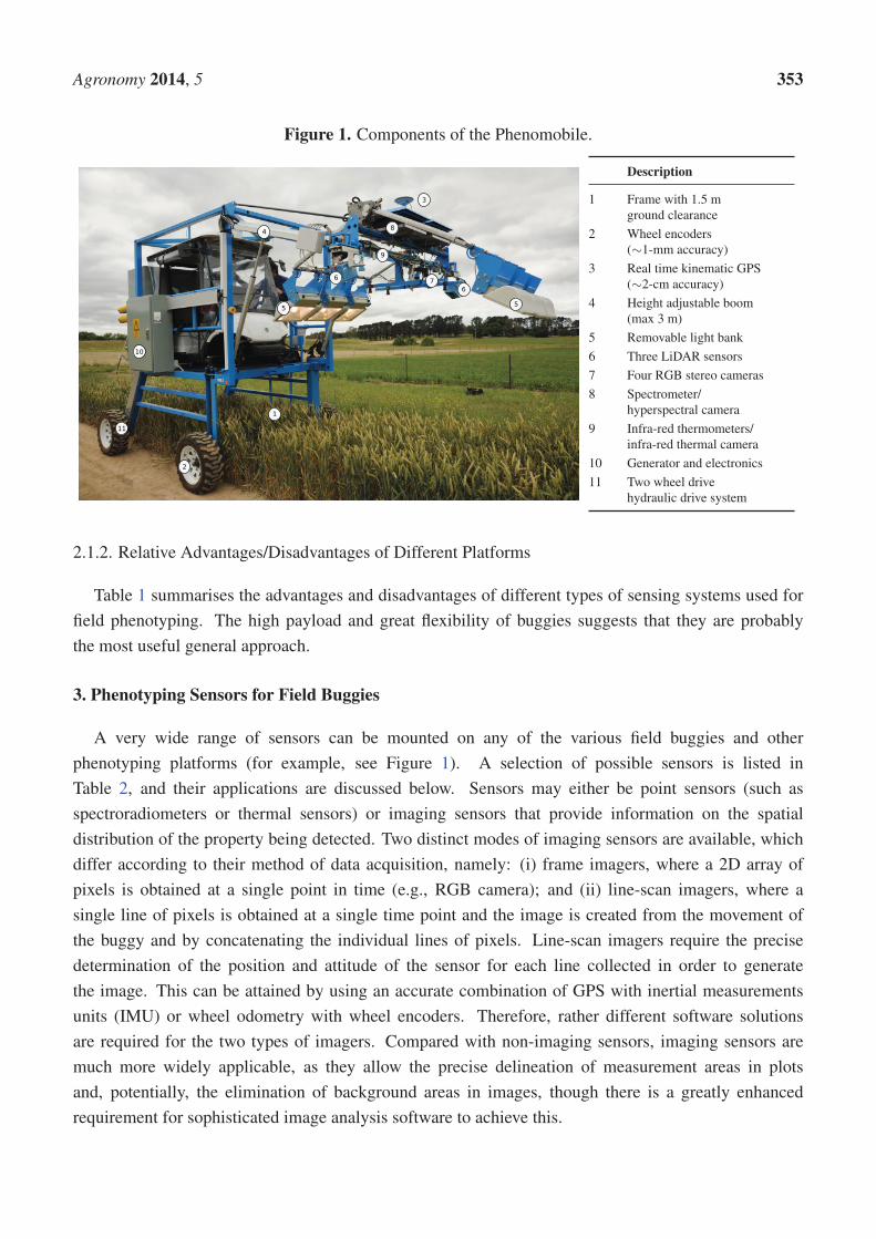
The Phenomobile developed at the High Resolution Plant Phenomics Centre, Canberra (Figure 1),

comprises a height adjustable sensor bar (max 3 m), a two-wheel drive hydraulic drive system, a 6-kW

generator, RTK GPS (∼2 cm resolution), wheel encoders on both front wheels (∼1 mm resolution) and a

removable light bank. The frame of the Phenomobile itself was designed to traverse a mature wheat crop

(1.2-m ground clearance) and the wheel width designed to match that of the equipment used to sow the

trials, thereby minimising the chance of encroachment into the experimental plot during measurement.

Thus, the Phenomobile can traverse ∼1.8-m width plots of a mature wheat crop without disturbing the

canopy at a typical operating speed of 1 m/s.

The height adjustable sensor bar can accommodate a range of sensors, including: three LiDAR

sensors, four high resolution RGB cameras, a thermal infra-red camera, three infra-red thermometers,

a full range spectroradiometer and a hyperspectral camera. Sample data sets from these sensors are

discussed in the below section within the context of the development of high-throughput phenotyping

techniques.

4.1.1. LiDAR Subsystem

The LiDAR subsystem used on the Phenomobile presents possibilities for using time of flight,

resolved distance, and signal intensity information to extract canopy structural parameters that are

traditionally measured either manually using destructive sampling or simply estimated by a visual score.

The LiDAR sensor (LMS400, 70◦ FOV, SICK AG, Waldkirch, Germany) used on the Phenomobile

comprises a monochromatic red laser light source. The active nature of the LiDAR confers a number of

advantages when compared to the traditional RGB camera, including: the LiDAR is not influenced by

shadows and changes in the ambient light conditions, while the RGB camera requires parameterization

for each light condition; the LiDAR can obtain measurements under all light conditions in contrast to

an RGB camera that requires an additional light source in low-light conditions.

The LiDAR intensity signal provides high contrast between soil and green vegetation, as a greater

proportion of the red laser is absorbed by green vegetation than soil. The high contrast between plant

and soil achieved from the LiDAR intensity image is highly amenable for image analysis to derive

ground cover estimation and possibly plant seedling counts. This is illustrated in the comparison of an

RGB image and a LiDAR intensity image of the same scene (Figure 2).

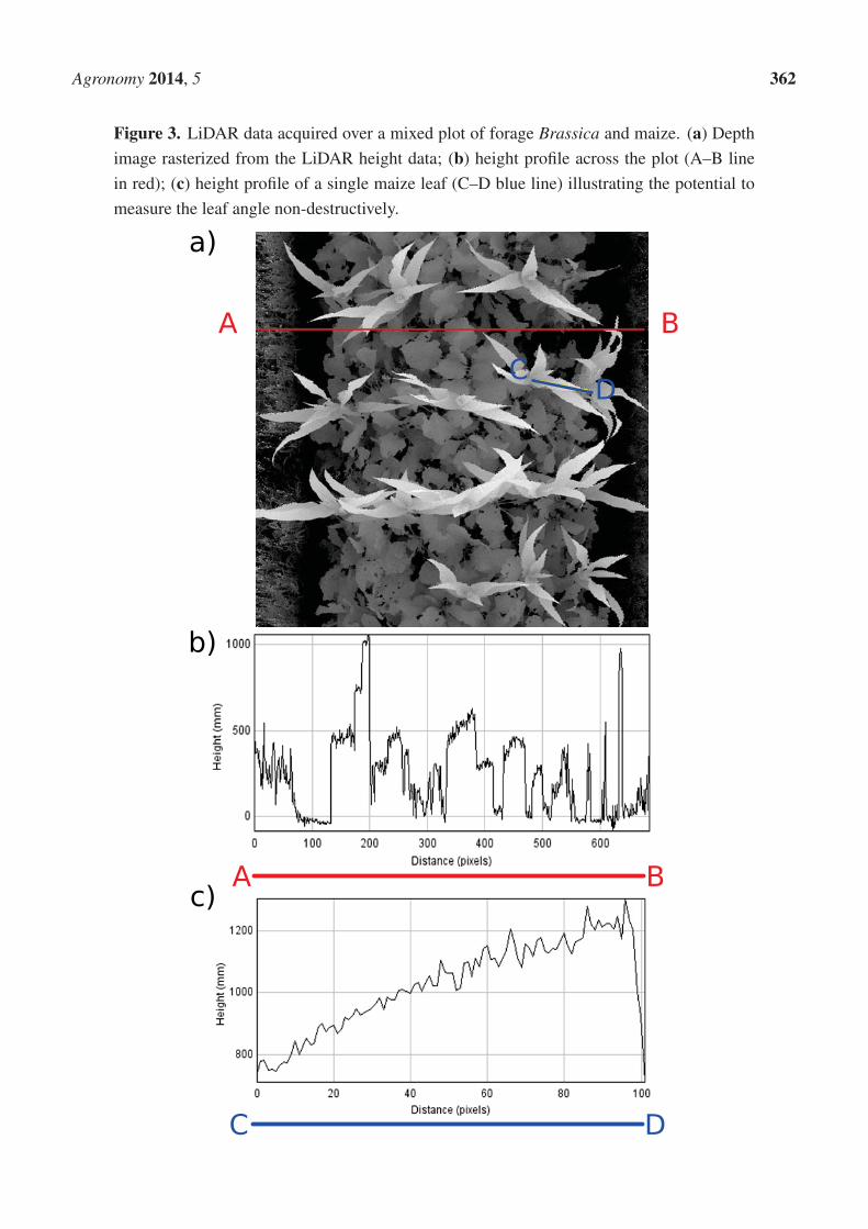
The high resolution of the height data obtained from the LiDAR is amenable to the estimation of

advanced canopy structural parameters, like leaf angular distribution. From the LiDAR height image

of a mixed plot of forage Brassica (Brassica napus) and maize (Zea mays), two transects have been

made in the image to derive the height profiles (Figure 3) across the width of the plot and for a single

maize leaf. The height profile of the single maize leaf illustrates the possibility for the non-destructive

estimation of leaf angle.

The time of flight returns from the LiDAR can be used to measure the height of the crop canopy.

This is illustrated in Figure 4 with the height profile of five genotypes varying for canopy height. The

two profiles show a single-pixel profile and the average height of the plot.

Agronomy 2014, 5 361

Figure 2. Comparison of an RGB image (a) and the intensity image from the LiDAR (b),

both acquired over the same plot of rice. The weeds and shadowing in the RGB image

present a clear difficulty for the automatic extraction of the fractional cover, while the use

of an active sensor, such as the red laser from the LiDAR, yields high contrast between soil

and plants and can even discriminate between species based on the intensity or pattern of the

reflectance.

�� ��

For an experiment comprising wheat genotypes varying for height, we compared the crop canopy

height measured manually with a ruler to the height extracted from the LiDAR data (Figure 5).

The manual measurements were obtained from one height measurement per 6 m by 2 m experimental

plot; while the LiDAR height measurements were obtained from the mean of the top 95th percentile

of the height distribution for a given experimental plot minus the height of the ground obtained from

the average of the returns from the soil. An R2 relationship of 0.86 was obtained between both

measurements with a root mean square error (RMSE) of 78.93 mm. Interestingly, for shorter canopy

height measurements, the LiDAR gave higher values than the manual measurement, while for taller

canopy height measurements, the LiDAR gave lower values than the manual measurement. The possible

explanation for this bias is that the manual measurements only sample one or two points of the plot using

the ruler, which in the case of non-uniform plots with a mix of tall and shorter plants could lead to a bias

in manual measurements.

The possibility to identify individual plant organs from the height image obtained from the LiDAR

is illustrated in Figure 6, where the spikes of a mature wheat crop are visible and have been segmented.

The segmentation of the canopy height and intensity images by depth could be used to further enhance

the contrast required for feature extraction of individual plant organs using image analysis algorithms.

Agronomy 2014, 5 362

Figure 3. LiDAR data acquired over a mixed plot of forage Brassica and maize. (a) Depth

image rasterized from the LiDAR height data; (b) height profile across the plot (A–B line

in red); (c) height profile of a single maize leaf (C–D blue line) illustrating the potential to

measure the leaf angle non-destructively.

��

��

��

� �

� �

�

�

Agronomy 2014, 5 363

Figure 4. Profile of the LiDAR elevation. The yellow line in the graph represents the profile of the single-pixel width transect across the

plots, denoted in yellow in the image; while the orange line in the graph represents the average height of all the pixels between the two

orange lines in the image.

0 500 1000 1500 2000 2500 3000 3500

Distance (pixels)

−200

0

200

400

600

800

1000

Hei

ght(mm

)

Single pixel profileAverage height between the two lines

0

100

200

300

400

500

600

700

800

900

Agronomy 2014, 5 364

Figure 5. Comparison of canopy height measured manually on wheat using the traditional ruler method and the height estimated with

the LiDAR. The resulting relationship shows R2 = 86 and RMSE = 78.93 mm.

200 400 600 800 1000 1200 1400

Manually measured canopy height (mm)

200

400

600

800

1000

1200

1400

LiD

AR

mea

sure

dca

nopy

heig

ht(m

m)

RMSE = 78.93mm

y = 230.77 + 0.66x R2 = 0.86

1:1 lineManual vs LiDAR

Agronomy 2014, 5 365

Figure 6. An example of the application of LiDAR for counting spikes in wheat. The

LiDAR elevation image (a) can be segmented into an image showing only the top fraction

of the image, which clearly shows the spikes (b). A simple particle count algorithm can be

used to count the number of elements per area.

�� ��

There are different approaches for processing and interpreting LiDAR data. The examples shown

above (Figures 3–6) deal with the information in the form of raster images. The returns of the LiDAR

are converted into distances and angles and then converted into an image. This has the advantage of

using standard image processing software for analysing the data. The alternative to this method is the

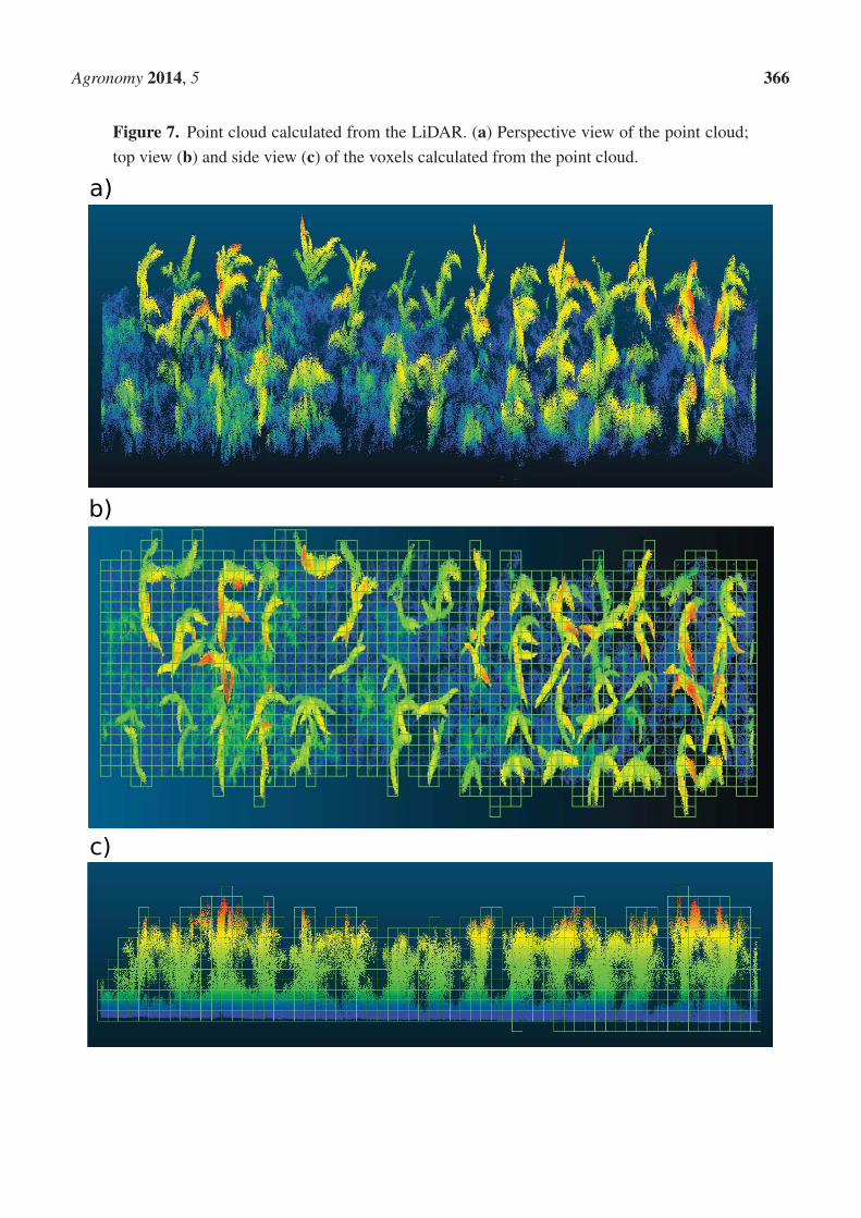
generation of point clouds with x, y, z coordinates associated with attributes, such as the intensity of

the return. Each return of the LiDAR is converted into a 3D point (Figure 7a). This requires specific

software to deal with the large number of point clouds generated from each LiDAR run. One way to deal

with the point cloud using standard image analysis software is to convert the point cloud into a voxel

image. A voxel (volume element) is the 3D equivalent to a pixel. Voxels are calculated by creating a grid

of cubes that overlap with the point cloud. For each of these cubes or voxels, it is possible to calculate

attributes, such as the number of returns, into the voxel or average intensity. Then, the resulting 3D array

of voxels can be exported as a multi-layered image that can be processed using most image analysis

software. The use of voxels is also amenable to the estimation of crop bio-volume and biomass or as the

input format for radiative transfer models [112,113].

Agronomy 2014, 5 366

Figure 7. Point cloud calculated from the LiDAR. (a) Perspective view of the point cloud;

top view (b) and side view (c) of the voxels calculated from the point cloud.

��

��

��

Agronomy 2014, 5 367

4.1.2. RGB Camera Subsystem

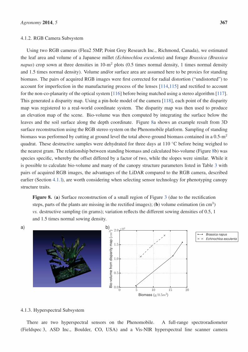
Using two RGB cameras (Flea2 5MP, Point Grey Research Inc., Richmond, Canada), we estimated

the leaf area and volume of a Japanese millet (Echinochloa esculenta) and forage Brassica (Brassicanapus) crop sown at three densities in 10-m2 plots (0.5 times normal density, 1 times normal density

and 1.5 times normal density). Volume and/or surface area are assumed here to be proxies for standing

biomass. The pairs of acquired RGB images were first corrected for radial distortion (“undistorted”) to

account for imperfection in the manufacturing process of the lenses [114,115] and rectified to account

for the non-co-planarity of the optical system [116] before being matched using a stereo algorithm [117].

This generated a disparity map. Using a pin-hole model of the camera [118], each point of the disparity

map was registered to a real-world coordinate system. The disparity map was then used to produce

an elevation map of the scene. Bio-volume was then computed by integrating the surface below the

leaves and the soil surface along the depth coordinate. Figure 8a shows an example result from 3D

surface reconstruction using the RGB stereo system on the Phenomobile platform. Sampling of standing

biomass was performed by cutting at ground level the total above-ground biomass contained in a 0.5-m2

quadrat. These destructive samples were dehydrated for three days at 110 ◦C before being weighed to

the nearest gram. The relationship between standing biomass and calculated bio-volume (Figure 8b) was

species specific, whereby the offset differed by a factor of two, while the slopes were similar. While it

is possible to calculate bio-volume and many of the canopy structure parameters listed in Table 3 with

pairs of acquired RGB images, the advantages of the LiDAR compared to the RGB camera, described

earlier (Section 4.1.1), are worth considering when selecting sensor technology for phenotyping canopy

structure traits.

Figure 8. (a) Surface reconstruction of a small region of Figure 3 (due to the rectification

steps, parts of the plants are missing in the rectified images); (b) volume estimation (in cm3)

vs. destructive sampling (in grams); variation reflects the different sowing densities of 0.5, 1

and 1.5 times normal sowing density.

0 5 10 15 20

Biomass (g/0.5m2)

0.0

0.5

1.0

1.5

2.0

Bio

-vol

ume

from

disp

arity

map

(cm

3) ×105

Brassica napusEchinochloa esculenta

a) b)

4.1.3. Hyperspectral Subsystem

There are two hyperspectral sensors on the Phenomobile. A full-range spectroradiometer

(Fieldspec 3, ASD Inc., Boulder, CO, USA) and a Vis-NIR hyperspectral line scanner camera

Agronomy 2014, 5 368

(Micro-Hyperspec, Headwall Photonics Inc., Fitchburg, MA, USA). The full-range spectroradiometer

is programmed to acquire continuous spectra at approximately 1 Hz that are geo-referenced using the

RTK GPS on the Phenomobile. A foreoptic of 18◦ FOV is installed on the optic fibre, providing an

80 mm diameter spot over the plot at a boom height of 2.5 m. The spectra are acquired in radiance

and then converted into reflectance using either a second full-range spectroradiometer fitted with the

cosine corrector and making continuous measurements of the incoming irradiance or using a radiative

transfer model to model irradiance from aerosol optical depth obtained from the NASA Aeronet station

in Canberra. Since each spectrum is geo-referenced, it is possible to extract the collection of spectra

corresponding to each plot. Then, a number of vegetation indices are calculated from the average plot

reflectances of the different spectral bands.

The hyperspectral camera can record images at a maximum frame rate of 90 Hz. The resolution of the

camera in the spatial axis is 1004 pixels, which, with the current foreoptics of 25◦ FOV and a 2.5-m boom

height, results in a 1.1-mm spatial resolution. However, the spatial resolution in the direction of travel is

determined by the speed of the Phenomobile and the frame rate of the camera. At the maximum frame

rate (90 Hz) and a travel speed of 1 m/s, the spatial resolution in the direction of travel is approximately

11 mm. Therefore, in order to get square pixels, it is required to travel at a lower speed or apply spatial

binning in order to reduce the spatial resolution on the axis perpendicular to the travel. Each scanned line

is time-tagged with GPS time, which is used for geo-referencing each line based on the information from

the RTK-GPS and wheel encoders on the Phenomobile. The camera is calibrated into radiance using a

uniform light source based on an integrating sphere (USS-2000S, Labsphere, North Sutton, NH, USA).

Then, the conversion into reflectance is similar to the one applied to the radiance measurements from

the full range spectroradiometer. The resulting image has 340 spectral bands with a spectral resolution

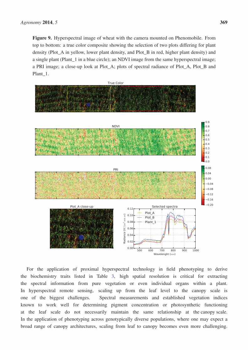
of approximately 2 nm. The example in Figure 9 shows a wheat experiment comprising two plots with

higher and lower plant density; Plot_A (denoted in yellow, lower plant density) and Plot_B (denoted in

red, higher plant density). The true color image is an RGB composite rendered using the visible bands.

From the hyperspectral image, it is possible to calculate a range of different vegetation indices. For

example, the NDVI and PRI are presented in Figure 9, whereby the average NDVI and PRI for the lower

plant density plot, Plot_A (0.58 and −0.047, respectively), is less than that for the higher plant density

plot, Plot_B (0.68 and −0.027, respectively).

Given the resolution of the hyperspectral system, it is possible to extract the reflectance from

individual plants and, thereby, discriminate between the individual plant organs, such as spikes and

flag leaves. See, for example, Figure 9, where Plant_1, denoted in blue, is the average reflectance of a

region of interest manually drawn over a single plant. In the case of incomplete canopies, where part of

the soil background is presented in the image, a simple NDVI-based mask can be used to filter out pixels

with low NDVI representing soil or shadows; therefore, only pixels with vegetation would be used in

the analysis.

Agronomy 2014, 5 369

Figure 9. Hyperspectral image of wheat with the camera mounted on Phenomobile. From

top to bottom: a true color composite showing the selection of two plots differing for plant

density (Plot_A in yellow, lower plant density, and Plot_B in red, higher plant density) and

a single plant (Plant_1 in a blue circle); an NDVI image from the same hyperspectral image;

a PRI image; a close-up look at Plot_A; plots of spectral radiance of Plot_A, Plot_B and

Plant_1.

For the application of proximal hyperspectral technology in field phenotyping to derive

the biochemistry traits listed in Table 3, high spatial resolution is critical for extracting

the spectral information from pure vegetation or even individual organs within a plant.

In hyperspectral remote sensing, scaling up from the leaf level to the canopy scale is

one of the biggest challenges. Spectral measurements and established vegetation indices

known to work well for determining pigment concentration or photosynthetic functioning

at the leaf scale do not necessarily maintain the same relationship at the canopy scale.

In the application of phenotyping across genotypically diverse populations, where one may expect a

broad range of canopy architectures, scaling from leaf to canopy becomes even more challenging.

Agronomy 2014, 5 370

The ability to extract the pixels from the hyperspectral image that represents the reflectance of a

well-illuminated leaf is only possible by using an imaging sensor with high spatial resolution. Moreover,

the combination of hyperspectral and the structural information obtained from the LiDAR will enable the

fusion of both datasets and permit the filtering of the spectral pixels on plant material to those with unique

sensor/sun geometry. This filtering technique can remove artifacts caused by differences in canopy

architecture and has been explored at the airborne level [119] over natural vegetation; therefore, the

same techniques that are applied with sub-metre imagery could be applied to sub-centimetre datasets

and single plants in field phenotyping.

4.1.4. Thermal Infrared Camera

The images captured by the thermal infrared camera (SC645, FLIR Systems Australia Pty Ltd,

Notting Hill, VIC, Australia) mounted on the Phenomobile contain sufficient resolution to identify

individual leaves in a wheat canopy (Figure 10). This level of resolution presents opportunities to

threshold soil from plant material and to overcome the complexities that arise from the influence of the

background soil temperature. Such complexities are increased when single pixel thermal infrared sensors

are used to measure the temperature of canopies with incomplete ground cover and row crops. Other

opportunities exist for identifying individual plant organs within the canopy to estimate transpiring and

non-transpiring plant material, as well as their relative contribution to the overall canopy transpiration at

a particular time during the growing season. Such an analysis could be used to evaluate traits contributing

to the duration of the grain-filling period in cereals, sometimes referred to as “stay green”, and to estimate

the transpiration of reproductive organs. However, to compare consecutive temperature measurements

of a large number of experimental plots, one must account for the influence of the changing environment

with time on the measured temperature (discussed previously in Section 3.1.5).

Figure 10. A single thermal image obtained with Phenomobile over wheat. The image

shows the contrast between the temperatures of the soil and the individual plants. In this

example, the soil was recently irrigated, and most of the soil is cooler than the actual canopy.

Agronomy 2014, 5 371

5. Conclusions

Obtaining useful information from proximal remote sensing buggies for use by breeders and

physiologists is a considerable challenge that has been identified by others [11]. For low-throughput

applications, like intensive physiology investigations, less automation and greater human intervention in

the data processing and analysis is acceptable. However, for commercial-scale breeding and pre-breeding

applications, mature data acquisition and automated data processing systems are required to keep pace

with the demand imposed by the large number of genotypes deployed across sites and environment types.

The latter application can often require expert level skills and capabilities in the software engineering and

computer science domains, necessitating genuine multidisciplinary collaborations to achieve substantive

outcomes. Multidisciplinary teams are required to overcome challenges with: hardware and software

integration; customization of data processing and analysis; efficient georeferencing of the data to an

experimental field plan and timely delivery of the data, preferably through secure web-based portals, to

inform decision-making. Today, the crop science community can leverage the unprecedented technology

advances made in computer science, image analysis, proximal remote sensing and robotics.

Acknowledgments

This work was funded through the National Collaborative Research Infrastructure Strategy

(Australian Plant Phenomics Facility) and the Grains Research and Development Corporation (CSP00148).

Allan Rattey supplied the manual measurements of crop canopy height shown in Figure 5. Xiao Tan

implemented the stereo reconstruction algorithm for Figure 8.

Author Contributions

David Deery, Jose Jimenez-Berni, Xavier Sirault and Robert Furbank conceived of, designed and

undertook the research presented in the case study. David Deery, Jose Jimenez-Berni and Hamlyn Jones

contributed to the overall conception and writing of the article with input and advice from Xavier Sirault

and Robert Furbank.

Conflicts of Interest

The authors declare no conflicts of interest.

References

1. Bruinsma, J. The resource outlook to 2050. By how much do land, water use and crop yields

need to increase by 2050? In Proceedings of the FAO Expert Meeting on How to Feed the World

in 2050, 24–26 June 2009; FAO: Rome, Italy, 2009.

2. Royal Society of London. Reaping the Benefits: Science and the Sustainable Intensification ofGlobal Agriculture; Technical Report; Royal Society: London, UK, 2009.

3. Tilman, D.; Balzer, C.; Hill, J.; Befort, B.L. Global food demand and the sustainable

intensification of agriculture. Proc. Natl. Acad. Sci. USA 2011, 108, 20260–20264.

Agronomy 2014, 5 372

4. Hall, A.; Wilson, M.A. Object-based analysis of grapevine canopy relationships with winegrape

composition and yield in two contrasting vineyards using multitemporal high spatial resolution

optical remote sensing. Int. J. Remote Sens. 2013, 34, 1772–1797.

5. Ingvarsson, P.K.; Street, N.R. Association genetics of complex traits in plants. New Phytol. 2011,

189, 909–922.

6. Rebetzke, G.; van Herwaarden, A.; Biddulph, B.; Moeller, C.; Richards, R.; Rattey, A.; Chenu, K.

Field Experiments in Crop Physiology, 2013. Available online: http://prometheuswiki.publish.csiro.au/

tiki-pagehistory.php?page=Field%20E%xperiments%20in%20Crop%20Physiology&preview=41

(accessed on 22 January 2014).

7. Pask, A.; Pietragalla, J.; Mullan, D.; Reynolds, M. Physiological Breeding II: A Field Guide toWheat Phenotyping; Technical Report; CIMMYT: Mexico, DF, Mexico, 2012.

8. Tuberosa, R. Phenotyping for drought tolerance of crops in the genomics era. Front. Physiol.2012, 3, doi:10.3389/fphys.2012.00347.

9. Cobb, J.N.; DeClerck, G.; Greenberg, A.; Clark, R.; McCouch, S. Next-generation phenotyping:

Requirements and strategies for enhancing our understanding of genotype-phenotype relationships

and its relevance to crop improvement. Theor. Appl. Genet. 2013, 126, 867–887.

10. Araus, J.L.; Cairns, J.E. Field high-throughput phenotyping: The new crop breeding frontier.

Trends Plant Sci. 2014, 19, 52–61.

11. White, J.W.; Andrade-Sanchez, P.; Gore, M.A.; Bronson, K.F.; Coffelt, T.A.; Conley, M.M.;

Feldmann, K.A.; French, A.N.; Heun, J.T.; Hunsaker, D.J.; et al. Field-based phenomics for plant

genetics research. Field Crops Res. 2012, 133, 101–112.

12. Cabrera-Bosquet, L.; Crossa, J.; von Zitzewitz, J.; Serret, M.D.; Araus, J.L. High-throughput

phenotyping and genomic selection: The frontiers of crop breeding converge. J. Integr. Plant Biol.2012, 54, 312–320.

13. Fussell, J.; Rundquist, D. On defining remote sensing. Photogramm. Eng. Remote Sens. 1986,

52, 1507–1511.

14. Fiorani, F.; Schurr, U. Future scenarios for plant phenotyping. Annu. Rev. Plant Biol. 2013, 64,

267–291.

15. Furbank, R.T.; Tester, M. Phenomics-technologies to relieve the phenotyping bottleneck. TrendsPlant Sci. 2011, 16, 635–644.

16. Walter, A.; Studer, B.; Kolliker, R. Advanced phenotyping offers opportunities for improved

breeding of forage and turf species. Ann. Bot. 2012, 110, 1271–1279.

17. Rebetzke, G.J.; Fischer, R.T.A.; van Herwaarden, A.F.; Bonnett, D.G.; Chenu, K.; Rattey, A.R.;

Fettell, N.A. Plot size matters: Interference from intergenotypic competition in plant phenotyping

studies. Funct. Plant Biol. 2013, 41, 107–118.

18. Amani, I.; Fischer, R.A.; Reynolds, M.F.P. Canopy Temperature Depression Association with

Yield of Irrigated Spring Wheat Cultivars in a Hot Climate. J. Agron. Crop Sci. 1996, 176, 119–129.

19. Brennan, J.P.; Condon, A.G.; van Ginkel, M.; Reynolds, M.P. An economic assessment of the

use of physiological selection for stomatal aperture-related traits in the CIMMYT wheat breeding

programme. J. Agric. Sci. 2007, 145, 187–194.

Agronomy 2014, 5 373

20. Condon, A.G.; Reynolds, M.P.; Rebetzke, G.J.; van Ginkel, M.; Richards, R.A.; Farquhar, G.D.

Using stomatal aperture-related traits to select for high yield potential in bread wheat. WheatProd. Stressed Environ. 2007, 12, 617–624.

21. Jones, H.G.; Serraj, R.; Loveys, B.R.; Xiong, L.; Wheaton, A.; Price, A.H. Thermal infrared

imaging of crop canopies for the remote diagnosis and quantification of plant responses to water

stress in the field. Funct. Plant Biol. 2009, 36, 978–989.

22. Prashar, A.; Yildiz, J.; McNicol, J.W.; Bryan, G.J.; Jones, H.G. Infra-red thermography for high

throughput field phenotyping in Solanum tuberosum. PLoS One 2013, 8, e65816.

23. Anderson, K.; Gaston, K.J. Lightweight unmanned aerial vehicles will revolutionize spatial

ecology. Front. Ecol. Environ. 2013, 11, 138–146.

24. Chapman, S.C.; Merz, T.; Chan, A.; Jackway, P.; Hrabar, S.; Dreccer, M.F.; Holland, E.;

Zheng, B.; Ling, T.J.; Jimenez-Berni, J. Pheno-Copter: A Low-Altitude, Autonomous

Remote-Sensing Robotic Helicopter for High-Throughput Field-Based Phenotyping. Agronomy2014, 4, 279–301.

25. Labbé, S.; Lebourgeois, V.; Virlet, N.; Martínez, S.; Regnard, J.L. Contribution of airborne

remote sensing to high- throughput phenotyping of a hybrid apple population in response to soil

water constraints. In Proceedings of the 2nd International Plant Phenotyping Symposium, Jülich,

Germany, 5–7 September 2011; International Plant Phenomics Network; pp. 185–191.

26. Matese, A.; Primicerio, J.; di Gennaro, F.; Fiorillo, E.; Vaccari, F.P.; Genesio, L. Development and

application of an autonomous and flexible unmanned aerial vehicle for precision viticulture. In

Acta Horticulturae; Poni, S., Ed.; International Society for Horticultural Science (ISHS): Leuven,

Belgium, 2013; pp. 63–69.

27. Perry, E.M.; Brand, J.; Kant, S.; Fitzgerald, G.J. Field-based rapid phenotyping with Unmanned

Aerial Vehicles (UAV). In Proceedings of 16th Agronomy Conference 2012, Armidale,

NSW, Australia, 14–18 October 2012; Australian Society of Agronomy: Armidale, NSW,

Australia, 2012.

28. Zarco-Tejada, P.; Berni, J.; Suárez, L.; Sepulcre-Cantó, G.; Morales, F.; Miller, J. Imaging

chlorophyll fluorescence with an airborne narrow-band multispectral camera for vegetation stress

detection. Remote Sens. Environ. 2009, 113, 1262–1275.

29. Zarco-Tejada, P.; González-Dugo, V.; Berni, J. Fluorescence, temperature and narrow-band

indices acquired from a UAV platform for water stress detection using a micro-hyperspectral

imager and a thermal camera. Remote Sens. Environ. 2012, 117, 322–337.

30. Zarco-Tejada, P.; Guillén-Climent, M.; Hernández-Clemente, R.; Catalina, A.; González, M.;

Martín, P. Estimating leaf carotenoid content in vineyards using high resolution hyperspectral

imagery acquired from an unmanned aerial vehicle (UAV). Agric. For. Meteorol. 2013, 171–172,

281–294.

31. LemnaTec GmbH. Scanalyzer Field—LemnaTec. Available online: http://www.lemnatec.com/

product/scanalyzer-field (accessed on 28 January 2014).

32. ETH Zurich. ETH—Crop Science—Field Phenotyping Platform (FIP). Available online:

http://www.kp.ethz.ch/infrastructure/FIP (accessed on 28 January 2014).

Agronomy 2014, 5 374

33. Romano, G.; Zia, S.; Spreer, W.; Sanchez, C.; Cairns, J.; Araus, J.L.; Müller, J. Use of

thermography for high throughput phenotyping of tropical maize adaptation in water stress.

Comput. Electron. Agric. 2011, 79, 67–74.

34. White, J.W.; Conley, M.M. A Flexible, Low-Cost Cart for Proximal Sensing. Crop Sci. 2013, 53,

1646–1649.

35. Ruckelshausen, A.; Biber, P.; Doma, M.; Gremmes, H.; Klose, R.; Linz, A.; Rahne, R.; Resch, R.;

Thiel, M.; Trautz, D.; et al. BoniRob: An autonomous field robot platform for individual

plant phenotyping. In Proceedings of the Joint International Agricultural Conference (2009),

Wageningen, Netherlands, 6–8 July 2009; van Henten, E.J., Goense, D., Lokhorst, C., Eds.;

Wageningen Agricultural Publishers: Wageningen, Netherlands, 2009; pp. 841–847.

36. Jensen, K.H.; Nielsen, S.H.; Jørgensen, R.N.; Bøgild, A.; Jacobsen, N.J.; Jørgensen, O.J.;

Jaeger-Hansen, C.H. A Low Cost, Modular Robotics Tool Carrier For Precision Agriculture

Research. In Proceedings of the 11th International Conference on Precision Agriculture,

Indianapolis, IN, USA, 15–18 July 2012; International Society of Precision Agriculture.

37. Andrade-Sanchez, P.; Gore, M.A.F.; Heun, J.T.; Thorp, K.R.; Carmo-Silva, A.E.; French, A.N.;

Salvucci, M.E.; White, J.W. Development and evaluation of a field-based high-throughput

phenotyping platform. Funct. Plant Biol. 2014, 41, 68–79.

38. Busemeyer, L.; Klose, R.; Linz, A.; Thiel, M.; Wunder, E.; Ruckelshausen, A. Agro-sensor

systems for outdoor plant phenotyping in low and high density crop field plots. In Proceedings

of the Landtechnik 2010—Partnerschaften für neue Innovationspotentiale, Düsseldorf, Germany,

27–28 October 2010; pp. 213–218.

39. Busemeyer, L.; Mentrup, D.; Möller, K.; Wunder, E.; Alheit, K.; Hahn, V.; Maurer, H.P.;

Reif, J.C.; Würschum, T.; Müller, J.; et al. BreedVision—A Multi-Sensor Platform for

Non-Destructive Field-Based Phenotyping in Plant Breeding. Sensors 2013, 13, 2830–2847.

40. Comar, A.; Burger, P.; de Solan, B.; Baret, F.; Daumard, F.; Hanocq, J.F. A semi-automatic system

for high throughput phenotyping wheat cultivars in-field conditions: Description and first results.

Funct. Plant Biol. 2012, 39, 914–924.

41. Casadesús, J.; Kaya, Y.; Bort, J.; Nachit, M.M.; Araus, J.L.; Amor, S.; Ferrazzano, G.;

Maalouf, F.; Maccaferri, M.; Martos, V.; et al. Using vegetation indices derived from conventional

digital cameras as selection criteria for wheat breeding in water-limited environments. Ann. Appl.Biol. 2007, 150, 227–236.

42. Jones, H.G.; Vaughan, R.A. Remote Sensing of Vegetation: Principles, Techniques, and Applications;

Oxford University Press: Oxford, UK, 2010; p. 369.

43. Lee, K.J.; Lee, B.W. Estimation of rice growth and nitrogen nutrition status using color digital

camera image analysis. Eur. J. Agron. 2013, 48, 57–65.

44. Liu, J.; Pattey, E. Retrieval of leaf area index from top-of-canopy digital photography over

agricultural crops. Agric. For. Meteorol. 2010, 150, 1485–1490.

45. Liu, L.; Peng, D.; Hu, Y.; Jiao, Q. A novel in situ FPAR measurement method for low canopy

vegetation based on a digital camera and reference panel. Remote Sens. 2013, 5, 274–281.

46. Baret, F.; de Solan, B.; Lopez-Lozano, R.; Ma, K.; Weiss, M. GAI estimates of row crops

from downward looking digital photos taken perpendicular to rows at 57.5◦ zenith angle:

Agronomy 2014, 5 375

Theoretical considerations based on 3D architecture models and application to wheat crops.

Agric. For. Meteorol. 2010, 150, 1393–1401.

47. Foucher, P.; Revollon, P.; Vigouroux, B.; Chassériaux, G. Morphological Image Analysis for the

Detection of Water Stress in Potted Forsythia. Biosyst. Eng. 2004, 89, 131–138.

48. Paproki, A.; Sirault, X.R.R.; Berry, S.; Furbank, R.T.; Fripp, J. A novel mesh processing based

technique for 3D plant analysis. BMC Plant Biol. 2012, 12, doi:10.1186/1471-2229-12-63.

49. Wang, H.; Zhang, W.; Zhou, G.; Yan, G.; Clinton, N. Image-based 3D corn reconstruction for

retrieval of geometrical structural parameters. Int. J. Remote Sens. 2009, 30, 5505–5513.

50. Huang, C.; Yang, W.; Duan, L.; Jiang, N.; Chen, G.; Xiong, L.; Liu, Q. Rice panicle length

measuring system based on dual-camera imaging. Comput. Electron. Agric. 2013, 98, 158–165.

51. Eitel, J.U.H.; Vierling, L.A.; Long, D.S.; Hunt, E.R. Early season remote sensing of wheat

nitrogen status using a green scanning laser. Agric. For. Meteorol. 2011, 151, 1338–1345.

52. Llorens, J.; Gil, E.; Llop, J.; Escolà, A. Ultrasonic and LIDAR sensors for electronic canopy

characterization in vineyards: Advances to improve pesticide application methods. Sensors 2011,

11, 2177–2194.

53. Sanz, R.; Rosell, J.; Llorens, J.; Gil, E.; Planas, S. Relationship between tree row LIDAR-volume

and leaf area density for fruit orchards and vineyards obtained with a LIDAR 3D Dynamic

Measurement System. Agric. For. Meteorol. 2013, 171–172, 153–162.

54. Gebbers, R.; Ehlert, D.; Adamek, R. Rapid Mapping of the Leaf Area Index in Agricultural Crops.

Agron. J. 2011, 103, 1532–1541.

55. Hosoi, F.; Omasa, K. Estimating vertical plant area density profile and growth parameters of a

wheat canopy at different growth stages using three-dimensional portable lidar imaging. ISPRSJ. Photogramm. Remote Sens. 2009, 64, 151–158.

56. Chéné, Y.; Rousseau, D.; Lucidarme, P.; Bertheloot, J.; Caffier, V.V.; Morel, P.; Belin, E.;

Chapeau-Blondeau, F.F.; Chene, Y.; Belin, E. On the use of depth camera for 3D phenotyping of

entire plants. Comput. Electron. Agric. 2012, 82, 122–127.

57. Klose, R.; Penlington, J.; Ruckelshausen, A. Usability of 3D time-of-flight cameras for automatic

plant phenotyping. Bornimer Agrartechnische Berichte 2011, 69, 93–105.

58. Azzari, G.; Goulden, M.L.; Rusu, R.B. Rapid characterization of vegetation structure with a

Microsoft Kinect sensor. Sensors 2013, 13, 2384–2398.

59. Aziz, S.A.; Steward, B.L.; Birrell, S.J.; Shrestha, D.S.; Kaspar, T.C. Ultrasonic Sensing for

Corn Plant Canopy Characterization. Paper Number 041120. In Proceedings of the 2004 ASAE

Annual Meeting, Ottawa, ON, Canada, 1–4 August 2004; American Society of Agricultural and

Biological Engineers, St. Joseph, Michigan; pp. 1–11.

60. Makeen, K.; Kerssen, S.; Mentrup, D.; Oeleman, B. Multiple Reflection Ultrasonic Sensor System

for Morphological Plant Parameters. Bornimer Agrartech. Berichte 2012, 78, 110–116.

61. Tucker, C.J. Red and photographic infrared linear combinations for monitoring vegetation.

Remote Sens. Environ. 1979, 8, 127–150.

62. Hilker, T.; Coops, N.C.; Coggins, S.B.; Wulder, M.A.; Brown, M.; Black, T.A.; Nesic, Z.;

Lessard, D. Detection of foliage conditions and disturbance from multi-angular high spectral

resolution remote sensing. Remote Sens. Environ. 2009, 113, 421–434.

Agronomy 2014, 5 376

63. Zarco-Tejada, P.; Berjón, A.; López-Lozano, R.; Miller, J.; Martín, P.; Cachorro, V.; González, M.;

de Frutos, A. Assessing vineyard condition with hyperspectral indices: Leaf and canopy

reflectance simulation in a row-structured discontinuous canopy. Remote Sens. Environ. 2005,

99, 271–287.

64. Zarco-Tejada, P.; Catalina, A.; González, M.; Martín, P. Relationships between net photosynthesis

and steady-state chlorophyll fluorescence retrieved from airborne hyperspectral imagery. RemoteSens. Environ. 2013, 136, 247–258.

65. Dreccer, M.F.; Barnes, L.R.; Meder, R. Quantitative dynamics of stem water soluble

carbohydrates in wheat can be monitored in the field using hyperspectral reflectance. Field CropsRes. 2014, 159, 70–80.

66. Darvishzadeh, R.; Skidmore, A.; Schlerf, M.; Atzberger, C.; Corsi, F.; Cho, M. LAI and

chlorophyll estimation for a heterogeneous grassland using hyperspectral measurements. ISPRSJ. Photogramm. Remote Sens. 2008, 63, 409–426.

67. Serbin, S.P.; Dillaway, D.N.; Kruger, E.L.; Townsend, P.A. Leaf optical properties reflect variation

in photosynthetic metabolism and its sensitivity to temperature. J. Exp. Bot. 2012, 63, 489–502.

68. Zhao, K.; Valle, D.; Popescu, S.; Zhang, X.; Mallick, B. Hyperspectral remote sensing of plant

biochemistry using Bayesian model averaging with variable and band selection. Remote Sens.Environ. 2013, 132, 102–119.

69. Römer, C.; Wahabzada, M.; Ballvora, A.; Pinto, F.; Rossini, M.; Panigada, C.; Behmann, J.;

Léon, J.; Thurau, C.; Bauckhage, C.; et al. Early drought stress detection in cereals: Simplex

volume maximisation for hyperspectral image analysis. Funct. Plant Biol. 2012, 39, 878–890.

70. Seiffert, U.; Bollenbeck, F.; Mock, H.P.; Matros, A. Clustering of crop phenotypes by means of

hyperspectral signatures using artificial neural networks. In Proceedings of the 2nd Workshop

Hyperspectral Image and Signal Processing: Evolution in Remote Sensing (WHISPERS),

Reykjavik, Iceland, 14–16 June 2010; IEEE; pp. 1–4.

71. Féret, J.B.; François, C.; Gitelson, A.; Asner, G.P.; Barry, K.M.; Panigada, C.; Richardson, A.D.;

Jacquemoud, S. Optimizing spectral indices and chemometric analysis of leaf chemical properties

using radiative transfer modeling. Remote Sens. Environ. 2011, 115, 2742–2750.

72. Garrity, S.R.; Eitel, J.U.H.; Vierling, L.A. Disentangling the relationships between plant

pigments and the photochemical reflectance index reveals a new approach for remote estimation

of carotenoid content. Remote Sens. Environ. 2011, 115, 628–635.

73. Serrano, L.; González-Flor, C.; Gorchs, G. Assessment of grape yield and composition using the

reflectance based Water Index in Mediterranean rainfed vineyards. Remote Sens. Environ. 2012,

118, 249–258.

74. Thiel, M.; Rath, T.; Ruckelshausen, A. Plant moisture measurement in field trials based on NIR

spectral imaging: A feasibility study. In Proceedings of the CIGR Workshop on Image Analysis

in Agriculture, Budapest, Hungary, 26–27 August 2010; Commission Internationale du Genie

Rural: Budapest, Hungary; pp. 16–29.

75. Yi, Q.X.; Bao, A.M.; Wang, Q.; Zhao, J. Estimation of leaf water content in cotton by means of

hyperspectral indices. Comput. Electron. Agric. 2013, 90, 144–151.

Agronomy 2014, 5 377

76. Gaulton, R.; Danson, F.M.; Ramirez, F.A.; Gunawan, O. The potential of dual-wavelength laser

scanning for estimating vegetation moisture content. Remote Sens. Environ. 2013, 132, 32–39.

77. Cheng, T.; Rivard, B.; Sánchez-Azofeifa, A. Spectroscopic determination of leaf water content

using continuous wavelet analysis. Remote Sens. Environ. 2011, 115, 659–670.

78. Ullah, S.; Schlerf, M.; Skidmore, A.K.; Hecker, C. Identifying plant species using mid-wave

infrared (2.5–6 μm) and thermal infrared (8–14 μm) emissivity spectra. Remote Sens. Environ.2012, 118, 95–102.

79. Ullah, S.; Skidmore, A.K.; Groen, T.A.; Schlerf, M. Evaluation of three proposed indices for the

retrieval of leaf water content from the mid-wave infrared (2–6 μm) spectra. Agric. For. Meteorol.2013, 171-172, 65–71.

80. De Bei, R.; Cozzolino, D.; Sullivan, W.; Cynkar, W.; Fuentes, S.; Dambergs, R.; Pech, J.; Tyerman, S.

Non-destructive measurement of grapevine water potential using near infrared spectroscopy.

Aust. J. Grape Wine Res. 2011, 17, 62–71.

81. Elsayed, S.; Mistele, B.; Schmidhalter, U. Can changes in leaf water potential be assessed

spectrally? Funct. Plant Biol. 2011, 38, 523–533.

82. Jones, H.G. The use of indirect or proxy markers in plant physiology. Plant, Cell Environ. 2014,

37, 1270–1272.

83. Gamon, J.A.; Peñuelas, J.; Field, C.B. A narrow-waveband spectral index that tracks diurnal

changes in photosynthetic efficiency. Remote Sens. Environ. 1992, 41, 35–44.

84. Kolber, Z.; Klimov, D.; Ananyev, G.; Rascher, U.; Berry, J.; Osmond, B. Measuring photosynthetic

parameters at a distance: Laser induced fluorescence transient (LIFT) method for remote

measurements of photosynthesis in terrestrial vegetation. Photosynth. Res. 2005, 84, 121–129.

85. Perez-Priego, O.; Zarco-Tejada, P.; Miller, J.; Sepulcre-Canto, G.; Fereres, E. Detection of

water stress in orchard trees with a high-resolution spectrometer through chlorophyll fluorescence

In-Filling of the O2-A band. IEEE Trans. Geosci. Remote Sens. 2005, 43, 2860–2869.

86. Guanter, L.; Alonso, L.; Gómez-Chova, L.; Amorós, J.; Vuila, J.; Moreno, J. A method for

detection of solar-induced vegetation fluorescence from MERIS FR data. In Proceedings of

the Envisat Symposium 2007, Montreux, Switzerland, 23–27 April 2007; ESA Communication

Production Office: Montreux, Switzerland, 2007.

87. Liu, L.; Zhang, Y.; Jiao, Q.; Peng, D. Assessing photosynthetic light-use efficiency using a

solar-induced chlorophyll fluorescence and photochemical reflectance index. Int. J. Remote Sens.2013, 34, 4264–4280.

88. Meroni, M.; Rossini, M.; Guanter, L.; Alonso, L.; Rascher, U.; Colombo, R.; Moreno, J. Remote

sensing of solar-induced chlorophyll fluorescence: Review of methods and applications. RemoteSens. Environ. 2009, 113, 2037–2051.

89. Mirdita, V.; Reif, J.C.; Ibraliu, A.; Melchinger, A.E.; Montes, J.M. Laser-induced fluorescence of

maize canopy to determine biomass and chlorophyll concentration at early stages of plant growth.

Albanian J. Agric. Sci. 2011, 10, 1–7.

90. Jones, H.G. Application of Thermal Imaging and Infrared Sensing in Plant Physiology and

Ecophysiology. Adv. Bot. Res. 2004, 41, 107–163.

Agronomy 2014, 5 378

91. Jiménez-Bello, M.; Ballester, C.; Castel, J.; Intrigliolo, D. Development and validation of an

automatic thermal imaging process for assessing plant water status. Agric. Water Manag. 2011,

98, 1497–1504.

92. Leinonen, I.; Jones, H.G. Combining thermal and visible imagery for estimating canopy

temperature and identifying plant stress. J. Exp. Bot. 2004, 55, 1423–1431.

93. Wang, X.; Yang, W.; Wheaton, A.; Cooley, N.; Moran, B. Automated canopy temperature

estimation via infrared thermography: A first step towards automated plant water stress

monitoring. Comput. Electron. Agric. 2010, 73, 74–83.

94. Jones, H.G. Use of infrared thermography for monitoring stomatal closure in the field:

Application to grapevine. J. Exp. Bot. 2002, 53, 2249–2260.

95. Wang, X.; Yang Weiping, W.A.; Cooley, N.; Moran, B. Efficient registration of optical and IR

images for automatic plant water stress assessment. Comput. Electron. Agric. 2010, 74, 230–237.

96. Leinonen, I.; Grant, O.M.; Tagliavia, C.P.P.; Chaves, M.M.; Jones, H.G. Estimating stomatal

conductance with thermal imagery. Plant, Cell Environ. 2006, 29, 1508–1518.

97. Rebetzke, G.J.; Rattey, A.R.; Farquhar, G.D.; Richards, R.A.; Condon, A.T.G. Genomic regions

for canopy temperature and their genetic association with stomatal conductance and grain yield in

wheat. Funct. Plant Biol. 2013, 40, 14–33.

98. Saint Pierre, C.; Crossa, J.; Manes, Y.; Reynolds, M.P. Gene action of canopy temperature in

bread wheat under diverse environments. TAG (Theor. Appl. Genet.; Theor. Angew. Genet.)2010, 120, 1107–1117.

99. Romano, G.; Zia, S.; Spreer, W.; Cairns, J.; Araus, J.L.; MuÌLller, J. Rapid phenotyping of

different maize varieties under drought stress by using thermal images. In Proceedings of the

CIGR International Symposium on Sustainable Bioproduction—Water, Energy and Food, Tokyo,

Japan, 19–23 September 2011; CIGR (Commission Internationale du Genie Rural); p. 22B02.

100. Ballester, C.; Jiménez-Bello, M.; Castel, J.; Intrigliolo, D. Usefulness of thermography for plant

water stress detection in citrus and persimmon trees. Agric. For. Meteorol. 2013, 168, 120–129.

101. Winterhalter, L.; Mistele, B.; Jampatong, S.; Schmidhalter, U. High throughput phenotyping of

canopy water mass and canopy temperature in well-watered and drought stressed tropical maize

hybrids in the vegetative stage. Eur. J. Agron. 2011, 35, 22–32.

102. André, F.; van Leeuwen, C.; Saussez, S.; van Durmen, R.; Bogaert, P.; Moghadas, D.;

de Rességuier, L.; Delvaux, B.; Vereecken, H.; Lambot, S. High-resolution imaging of a vineyard

in south of France using ground-penetrating radar, electromagnetic induction and electrical

resistivity tomography. J. Appl. Geophys. 2012, 78, 113–122.

103. Noh, H.; Zhang, Q. Shadow effect on multi-spectral image for detection of nitrogen deficiency

in corn. Comput. Electron. Agric. 2012, 83, 52–57.

104. Suárez, L.; Zarco-Tejada, P.; Berni, J.; González-Dugo, V.; Fereres, E. Modelling PRI for water

stress detection using radiative transfer models. Remote Sens. Environ. 2009, 113, 730–744.

105. Malenovský, Z.; Mishra, K.B.; Zemek, F.; Rascher, U.; Nedbal, L. Scientific and technical

challenges in remote sensing of plant canopy reflectance and fluorescence. J. Exp. Bot. 2009, 60,

2987–3004.

Agronomy 2014, 5 379

106. Passioura, J.B. Grain Yield, Harvest Index, and Water Use of Wheat. J. Aust. Inst. Agric. Sci.1977, 43, 117–120.

107. Monteith, J.L. Climate and the Efficiency of Crop Production in Britain. Philos. Trans. R. Soc.Lond. B Biol. Sci. 1977, 281, 277–294.

108. Reynolds, M.; Tuberosa, R. Translational research impacting on crop productivity in

drought-prone environments. Curr. Opin. Plant Biol. 2008, 11, 171–179.

109. Richards, R.A.; Rebetzke, G.J.; Watt, M.; Condon, A.G.T.; Spielmeyer, W.; Dolferus, R. Breeding

for improved water productivity in temperate cereals: phenotyping, quantitative trait loci, markers

and the selection environment. Funct. Plant Biol. 2010, 37, 85–97.

110. Rebetzke, G.J.; Chenu, K.; Biddulph, B.; Moeller, C.; Deery, D.M.; Rattey, A.R.; Bennett, D.;

Barrett-Lennard, E.G.; Mayer, J.E. A multisite managed environment facility for targeted trait

and germplasm phenotyping. Funct. Plant Biol. 2013, 40, 1–13.

111. Sinclair, T.R.; Muchow, R.C. Radiation Use Efficiency. In Advances in Agronomy; Sparks, D.L.,

Ed.; Elsevier: Philadelphia, PA, USA, 1999; Volume 65, pp. 215–265.

112. Gastellu-Etchegorry, J.P.; Demarez, V.; Pinel, V.; Zagolski, F. Modeling radiative transfer in

heterogeneous 3-D vegetation canopies. Remote Sens. Environ. 1996, 58, 131–156.

113. Gastellu-Etchegorry, J.P.; Martin, E.; Gascon, F. DART: A 3D model for simulating satellite

images and studying surface radiation budget. Int. J. Remote Sens. 2004, 25, 73–96.

114. Brown, D.C. Close-range camera calibration. Photogramm. Eng. 1971, 37, 855–866.

115. Fryer, J.G.; Brown, D.C. Lens Distortion for Close-Range Photogrammetry. Photogramm. Eng.Remote Sens. 1986, 52, 51–58.

116. Trucco, E.; Verri, A. Introductory Techniques for 3-D Computer Vision; Prentice Hall PTR:

Upper Saddle River, NJ, USA, 1998.

117. Sun, C. Fast Stereo Matching Using Rectangular Subregioning and 3D Maximum-Surface

Techniques. Int. J. Comput. Vis. 2002, 47, 99–117.

118. Hartley, R.I.; Zisserman, A. Multiple View Geometry in Computer Vision, 2nd ed.; Cambridge

University Press: Cambridge, United Kingdom 2004; ISBN: 0521540518.

119. Asner, G.P.; Martin, R.E. Airborne spectranomics: Mapping canopy chemical and taxonomic

diversity in tropical forests. Front. Ecol. Environ. 2009, 7, 269–276.

c© 2014 by the authors; licensee MDPI, Basel, Switzerland. This article is an open access article

distributed under the terms and conditions of the Creative Commons Attribution license

(http://creativecommons.org/licenses/by/3.0/).