Kernel density estimation in R - University of New Mexicomath.unm.edu/~james/w7-STAT574b.pdfKernel...

Kernel density estimation in R

Kernel density estimation can be done in R using the density() functionin R. The default is a Guassian kernel, but others are possible also. It usesit’s own algorithm to determine the bin width, but you can override andchoose your own. If you rely on the density() function, you are limitedto the built-in kernels. If you want to try a different one, you have to writethe code yourself.

STAT474/STAT574 February 25, 2015 1 / 49

Kernel density estimation in R: effect of bandwidth forrectangular kernel


Kernel density estimation in R

Note that exponential densities are a bit tricky to estimate to using kernelmethods. Here is the default behavior estimating the density forexponential data.

> x <- rexp(100)

> plot(density(x))


Kernel density estimation in R: exponential data withGaussian kernel

There are better approaches for doing nonparametric estimation for anexponential density that are a bit beyond the scope of the course.


Violin plots: a nice application of kernel density estimation

Violin plots are an alternative to boxplots that show nonparametric densityestimates of the distribution in addition to the median and interquartilerange. The densities are rotated sideways to have a similar orientation as abox plot.

> x <- rexp(100)

> install.packages("vioplot")

> library(vioplot)

> x <- vioplot(x)


Kernel density estimation in R: violin plot


Kernel density estimation R: violin plot

The violin plot uses the function sm.density() rather than density()

for the nonparametric density estimate, and this leads to smoother densityestimates. If you want to modify the behavior of the violin plot, you cancopy the original code to your own function and change how thenonparametric density estimate is done (e.g., replacing sm.density withdensity, or changing the kernel used).







> vioplot

function (x, ..., range = 1.5, h = NULL, ylim = NULL, names = NULL,

horizontal = FALSE, col = "magenta", border = "black", lty = 1,

lwd = 1, rectCol = "black", colMed = "white", pchMed = 19,

at, add = FALSE, wex = 1, drawRect = TRUE)

{

datas <- list(x, ...)

n <- length(datas)

if (missing(at))

at <- 1:n

upper <- vector(mode = "numeric", length = n)

lower <- vector(mode = "numeric", length = n)

q1 <- vector(mode = "numeric", length = n)

q3 <- vector(mode = "numeric", length = n)

...

args <- list(display = "none")

if (!(is.null(h)))

args <- c(args, h = h)

for (i in 1:n) {

...

smout <- do.call("sm.density", c(list(data, xlim = est.xlim),

args))


Kernel density estimation

There are lots of popular Kernel density estimates, and statisticians haveput a lot of work into establishing their properties, showing when someKernels work better than others (for example, using mean integratedsquare error as a criterion), determining how to choose bandwidths, and soon.

In addition to the Guassian, common choices for the hazard functioninclude

I Uniform, K (u) = 1/2 I (−1 ≤ u ≤ 1)

I Epanechnikov, K (u) = .75(1− u2)I (−1 ≤ u ≤ 1)

I biweight, K (u) = 1516(1− x2)2I (−1 ≤ u ≤ 1)


Kernel-smoothed hazard estimation

To estimate a smoothed version of the hazard function using a kernalmethod, first pick a kernel, then use

h =1

b

D∑i=1

K

(t − tib

)∆H(ti )

where D is the number of death times and b is the babdwidth (instead ofh). A common notation for bandwidth is h, but we use b because h isused for the hazard function. Also H(t) is the Nelson-Aalen estimator ofthe cumulative hazard function:

H(t) =

{0, if t ≤ t1∑

ti≤tdiYi, if t > t1


Kernel-smoothed hazard estimation

The variance of the smoothed hazard is

σ2[h(t)] = b−2D∑i=1

[K

(t − tib

)]2∆V [H(t)]


Asymmetric kernels

A difficulty that we saw with the exponential also can occur here, theestimated hazard can give negative values. Consequently, you can use anasymmetric kernel instead for small t.

For t < b, let q = t/b. A similar approach can be used for large t, whentD − b < t < tD . In this case, you can use q = (tD − t)/b and replace xwith −x in the kernal density estimate for these larger times.


Asymmetric kernels


Asymmetric kernels


Confidence intervals

A pointwise confidence interval can be obtained with lower and upperlimits (

h(t) exp

[−Z1−α/2σ(h(t))

h(t)

], h(t) exp

[Z1−α/2σ(h(t))

h(t)

])

Note that the confidence interfal is really a confidence interval for thesmoothed hazard function and not a confidence interval for the actualhazard function, making it difficult to interpret. In particular, theconfidence interval will depend on the both the kernel and the bandwidth.Coverage probabilities for smoothed hazard estimates (the proportion oftimes the confidence interval includes the true hazard rate) appears tohave ongoing research.


Asymmetric kernels


Effect of bandwidth


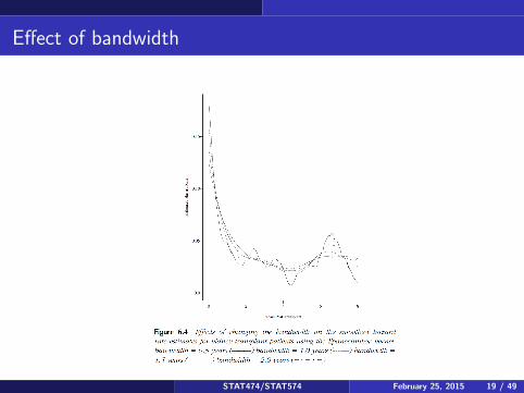
Effect of bandwidth

Because the bandwidth has a big impact, we somehow want to pick theoptimal bandwidth. An idea is to minimize the squared area between thetrue hazard function and estimated hazard function. This squared areabetween the two functions is called the Mean Integrated Squared Error(MISE):

MISE (b) = E

∫ τU

τL

[h(u)− h(u)]2 du

= E

∫ τU

τL

h2(u) du − 2E

∫ τU

τL

h(u)h(u) du + f (h(u))

The last term doesn’t depend on b so it is sufficient to minimize thefunction ignoring the last term. The first term can be estimated by∫ τUτL

h2(u) du, which can be estimated using the trapezoid rule fromcalculus.


Effect of bandwidth

The second term can be approximated by

1

b

∑i 6=j

K

(t − tib

)∆H(ti )∆H(tj)

summing over event times between τL and τU . Minimizing MISE is can bedone approximately by minimizing

g(b) =∑i

(ui+1 − ui

2

)[h2(ui )− h2(ui+1)]− 2

b

∑i 6=j

K

(t − tib

)∆H(ti )∆H(tj)

The minimization can be done numerically by plugging in different valuesof b and evaluating.


Effect of bandwidth


Effect of bandwidth

For this example, the minimum occurs around b = 0.17 to b = 0.23depending on the kernel.

Generally, there is a trade-off with smaller bandwidths having smaller biasbut higher variance, and larger bandwidths (more smoothing) having lessvariance but greater bias. Measuring the quality of bandwidths and kernelsusing MISE is standard in kernel density estimation (not just survivalanalysis). Bias here means that E [h(t)] 6= h(t).


Section 6.3: Estimation of Excess Mortality

The idea for this topic is to compare the survival curve or hazard rate forone group against a reference group, particular if the non-reference groupis thought to have higher risk. The reference group might come from amuch larger sample, so that its survival curve can be considered to beknown.

An example is to compare the mortality for psychiatric patients against thegeneral population. You could use census data to get the lifetable for thegeneral population, and determine the excess mortality for the psychiatricpatients. Two approaches are: a multiplicative model, and an additivemodel. In the multiplicative model, belonging to a particular groupmultiplies the hazard rate by a factor. In the additive model, belonging toa particular group adds a factor to the hazard rate.


Excess mortality

For the multiplicative model, if there is a reference hazard rate of θj(t) forthe jth individual in a study (based on sex, age, ethnicity, etc.), then dueto other risk factors, the hazard rate for the jth individual is

hj(t) = β(t)θj(t)

where β(t) ≥ 1 implies that the hazard rate is higher than the referencehazard. We define

B(t) =

∫ t

0β(u) du

as the cumulative relative excess mortality.


Excess mortality

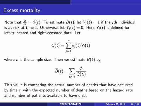
Note that ddt = β(t). To estimate B(t), let Yj(t) = 1 if the jth individual

is at risk at time t. Otherwise, let Yj(t) = 0. Here Yj(t) is defined forleft-truncated and right-censored data. Let

Q(t) =n∑

j=1

θj(t)Yj(t)

where n is the sample size. Then we estimate B(t) by

B(t) =∑ti≤t

diQ(ti )

This value is comparing the actual number of deaths that have occurredby time ti with the expected number of deaths based on the hazard rateand number of patients available to have died.


Excess mortality

The variance is estimated by

V [B(t)] =∑ti≤t

diQ(ti )2

β(t) can be estimated by slope of B(t), which can be improved by usingkernel-smoothing methods on B(t).


Excess mortality

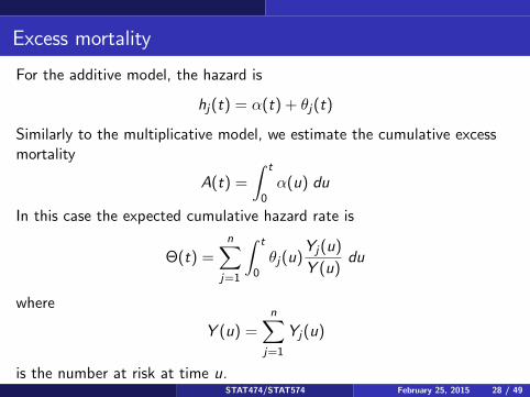
For the additive model, the hazard is

hj(t) = α(t) + θj(t)

Similarly to the multiplicative model, we estimate the cumulative excessmortality

A(t) =

∫ t

0α(u) du

In this case the expected cumulative hazard rate is

Θ(t) =n∑

j=1

∫ t

0θj(u)

Yj(u)

Y (u)du

where

Y (u) =n∑

j=1

Yj(u)

is the number at risk at time u.STAT474/STAT574 February 25, 2015 28 / 49

Excess mortality

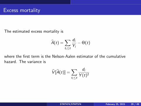
The estimated excess mortality is

A(t) =∑ti≤t

diYi−Θ(t)

where the first term is the Nelson-Aalen estimator of the cumulativehazard. The variance is

V [A(t)] =∑ti≤t

diY (t)2


Excess mortality

For a lifetable where times are every year, you can also compute

Θ(t) = Θ(t − 1) +∑t

λ(aj + t − 1)

Y (t)

where aj is the age at the beginning of the study for patient j and λ is the

reference hazard. Note that Θ(t) is a smooth function of t while A(t) ishas jumps.


Excess mortality

A more general model is to combine multiplicative and additivecomponents, using

hj(t) = β(t)θj(t) + α(t)

which is done in chapter 10.


Example: Iowa psychiatric patients

As an example, starting with the multiplicative model, consider 26psychiatric patients from Iowa, where we compare to census data.


Iowa psychiatric patients


Census data for Iowa


Excess mortality for Iowa psychiatric patients


Excess mortality for Iowa psychiatric patients


Excess mortality

The cumulative excess mortality is difficult to interpret. The slope of thecurve is more meaningful. The curve is relatively linear. If we consider age10 to age 30, the curve goes from roughly 50 to 100, suggesting a slope of(100− 50)/(30− 10) = 2.5, so that patients aged 10 to 30 had a roughly2.5 times higher chance of dying.

This is a fairly low-risk age group, for which suicide is high risk factor.Note that the census data might include psychiatric patients who havecommitted suicide, so we might be comparing psychiatric patients to thegeneral population which includes psychiatric patients, as opposed topsychiatric patients compared to people who have not been psychiatricpatients, so this might bias results.


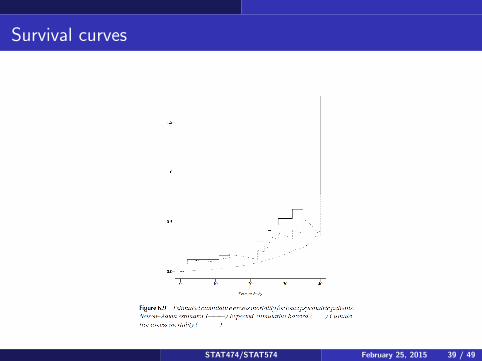
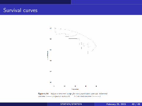
Survival curves

You can use the reference distribution to inform the survival curve insteadof just relying on the data. This results in an adjusted or corrected survivalcurve. Let S∗(t) = exp[−Θ(t)] (or use the cumulative hazard based onmultiplying the reference hazard by the excess harzard) and let S(t) be thestandard Kaplan-Meier survival curve (using only the data, not thereference survival data). Then Sc(t) = S(t)/S∗(t) is the correctedsurvival function. The estimate can be greater than 1, in which case theestimate can be set to 1.Typically, S∗(t) is less than 1, so that dividing by this quantity increasesthe estimated survival probabilities. This is somewhat similar in Bayesianstatististics to the use of the prior, using the reference survival times as aprior for what the psychiatric patients are likely to experience.Consequently, the adjusted survival curve is in between the kaplan-meier(data only) estimate, and the reference survival times.


Survival curves


Survival curves


Bayesian nonparametric survival analysis

The previous example leads naturally to Bayesian nonparametric survivalanalysis. Here we have prior information (or prior beliefs) about the shapeof the survival curve (such as based on a reference survival function). Thesurvival curve based on this previous information is combined with thelikelihood of the survival data to produce a posterior estimate of thesurvival function.

Reasons for using a prior are: (1) to take advantage of prior information orexpertise of someone familiar with the type of data, (2) to get areasonable estimate when the sample size is small.


Bayesian survival analysis

In frequentist statistical methods, parameters are treated as fixed, butunknown, and an estimator is chosen to estimate the parameters based onthe data and a model (including model assumptions). Parameters areunknown, but are treated as not being random.

Philosophically, the Bayesian approach is to try to model all uncertaintyusing random variables. Uncertainty exists both in the form of the datathat would arise from a probability model as well as the parameters of themodel itself, so both observations and parameters are treated as random.Typically, the observations have a distribution that depends on theparameters, and the parameters themselves come from some otherdistribution. Bayesian models are therefore often hierarchical, often withmultiple levels in the hierarchy.



For survival analysis, we think of the (unknown) survival curve as theparameter. From a frequentist point of view, survival probabilitiesdetermine the probabilities of observing different death times, but thereare no probabilities of the survival function itself.

From a Bayesian point of view, you can imagine that there was somestochastic process generating survival curves according to some distributionon the space of survival curves. One of the survival curves happened tooccur for the population we are studying. Once that survival function waschosen, event times could occur according to that survival curve.





We imagine that there is a true survival curve S(t), and an estimatedsurvival curve, S(t). We define a loss function as

L(S , S) =

∫ ∞0

[S(t)− S(t)]2 dt

The function S that minimizes the expected value of the loss function iscalled the posterior mean, which is used to estimate the survival function.


A prior for survival curves

A typical way to assign a prior on the survival function is to use a Dirichletprocess prior. For a Dirichlet process, we partition the real line intointervals A1, . . . ,Ak , so that P(X ∈ Ai ) = Wi . The numbers(W1, . . . ,Wk) have a k-dimension Dirichlet distribution with parametersα1, . . . , αk . For this to be a Dirichlet distribution, we must have Zi ,i = 1, . . . , k are independent gamma random variables with shapeparameter αi and Wi = Zi∑k

i=1 Zi. By construction, the random numbers

W ′i s are between 0 and 1 and sum to 1, so when interpreted as

probabilities, they form a discrete probability distribution.

Essentially, we can think of a Dirichlet distribution as a distribution onunfair dice with k sides. We want to make a die that has k sides, and wewant the probabilities of each side to be randomly determined. How fair orunfair the die is partly depends on the α parameters and partly depends onchance itself.


A prior for survival curves

We can also think of the Dirichlet distrbibution as generalizing the betadistribution. A beta random variable is a number between 0 and 1. Thisnumber partitions the interval [0,1] into two pieces, [0, x) and [x , 1]. ADirichlet random variable partitions the interval into k regions, using k − 1values between 0 and 1. The joint density for these k − 1 values is

f (w1, . . . ,wk−1) =Γ[α1 + · · ·+ αk)

Γ(α1) · · · Γ(αk)

[k−1∏i=1

wαi−1i

][1−

k−1∑i=1

wi

]αk−1

which reduces to a beta density with parameters (α1, α2) when k = 2.


Assigning a prior

To assign a prior on the space of survival curves, first assume an averagesurvival function, S0(t). The Dirichlet prior determines when the jumpsoccur, and the exponential curve gives the decay of the curve betweenjumps. Simulated survival curves when S0(t) = e−0.1t and α = 5S0(t) aregiven below.





Other approaches are to have a prior for the cumulative hazard functionand to use Gibb’s sampling or Markov chain Monte Carlo. These topicswould be more appropriate to cover after a class in Bayes methods.


Date post:	10-May-2018
Category:	Documents
Upload:	lytram
View:	223 times
Download:	1 times

Kernel density estimation in R - University of New Mexicomath.unm.edu/~james/w7-STAT574b.pdfKernel...

Documents