Yang Ma, Mariush W. Kemblowski and Gilberto E. UrrozDepartment of Civil and Environmental EngineeringUtah Water Research LaboratoryUtah State UniversityLogan, Utah
Abstract
Kinematic mixing theory is used to analyze reactive transport in randomvelocity fields. The theoretical results indicate that the field-scale reaction rateis strongly related to the spatial structure of the velocity field, which in turn isrelated to the autocovariance of logK. The theoretical results are verified bynumerical experiments.
1 Introduction
In real world environment protection practice, one of the most frequentlyasked questions is "How far will a contaminant plume migrate before itbiodegrades?". To predict the plume behavior, it is necessary to estimate: (1)the rate of migration; and (2) the rate of biodegradation. The rate ofcontaminant migration can be estimated by measuring the hydraulic gradientand permeability of the aquifer. Accurate estimation of the biodegradation ratewithin an aquifer is much more difficult. Results from laboratory microcosmstudies are sometimes an order of magnitude greater than the rates estimatedfrom the field mass balance data. For example, at a gas plant site in MichiganChiang [1]; Chiang [2], mass balance data yielded a first-order BTXdegradation rate of 0.0092/day, while 0.085/day was the value measured inlaboratory studies using the same soil. Similarly, at a gas station in FloridaKemblowski [3], the field estimate was 0.0085/day and the laboratorymicrocosm value was 0.036/day.
A similar observation was also made based on the analysis of a carefullydesigned API field investigation during a 16-month period from 1988 to 1989at Borden, Ontario, Hubbert [4]. In conjunction with the field investigation, anassociated set of laboratory experiments was also conduced. Table 1 shows thefirst-order degradation rates for the field study and the laboratory microcosmexperiment. It is apparent that all gasoline constituents, benzene, toluene,ethylbenzene and xylene, have higher mass loss rates at the lab scale than atthe field scale.
In order to explain the discrepancies between biodegradation ratesmeasured in laboratory microcosm studies and estimates from field massbalance data, we will first observe the behavior of a typical field hydrocarboncontaminant plume in groundwater.
104 Measurements and Modelling in Environmental Pollution
Table 1. Comparison of First Order Mass Loss Rates (day*)
SoluteBenzeneToluene
Ethylbenzenep-Xylenem-Xylene0-Xylene
100% PS-6(Field)0.0040.0130.0080.0070.0100.006
100% PS-6(Lab)0.0240.0370.0310.0250.0380.030
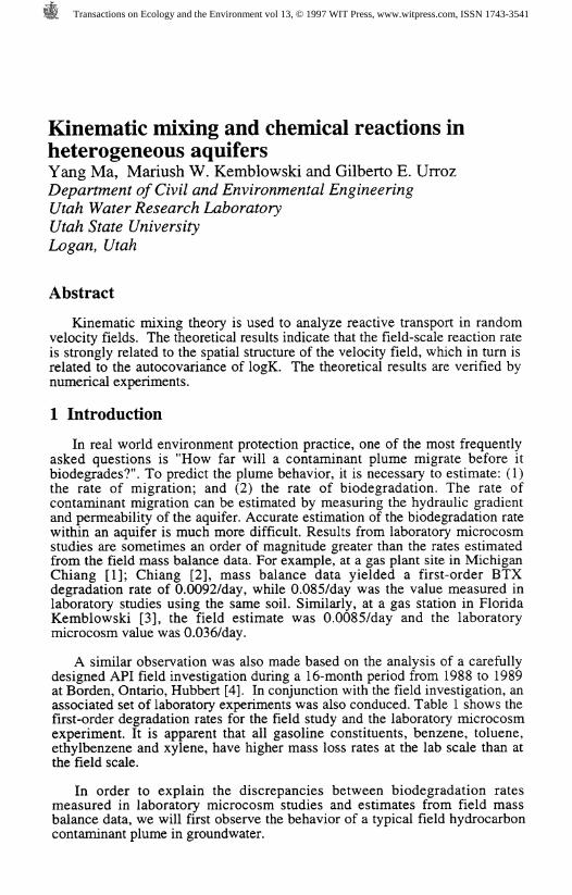
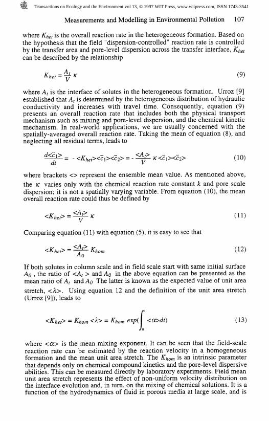
Figure 1 shows a simple schematic plan view of a field-dissolved hydrocarbonplume undergoing biodegradation. Dissolved hydrocarbons migratedowngradient from the source area. Native microorganisms will use theavailable oxygen in the source area to biodegrade a small portion of thehydrocarbon. The remaining hydrocarbons that are not initially biodegradedwill then be carried downgradient in a plume of anaerobic contaminated water.As the plume moves downgradient, dispersion will mix the anaerobichydrocarbon-contaminated water with clean oxygenated water at the plumefringes. This is the region where most aerobic biodegradation occurs. Thus, asthe dissolved hydrocarbons spread, they come in contact with oxygenatedgroundwater, and are subsequently degraded.
Oxygenated- UncontaminatedGroundwater
Flo*
Flow
Oxygenated- UncontaminatedGroundwater
Figure 1. Plan view of a typical hydrocarbon plume undergoing naturalbiodegradation. After Borden [5].
The major limitations to this process are the amount of ambient oxygen presentand the rate of mixing. Recent field results, Freyberg [6]; Patrick [7];Moltyaner [8]; Hubbert [4] have shown that mixing in most aquifers is verylimited, and, consequently, the transport of oxygen into dissolved hydrocarbonplumes becomes the rate-limiting factor in biodegradation. On the other hand,in the laboratory-based microcosm studies, sampled hydrocarbons are fullymixed with oxygen. Oxygen availability in the latter case is sufficient to allowaerobic biodegradation without oxygen becoming a rate-limiting factor. As aresult, the overall biodegradation rates measured in laboratory microcosmstudies are much higher than the rates estimated from field investigations.
Measurements and Modelling in Environmental Pollution 105
Since a thorough field investigation of every specific contaminant site ispractically impossible, it becomes very important to find a new model thatestimates the field biodegradation rate. This model should reflect the impact ofthe aquifer heterogeneities on biodegradation, and specifically on the mixing ofhydrocarbons with oxygenated water, and also be capable of utilizing theintrinsic kinetic properties of reaction measured by the laboratory experiments.
In the following sections we will first discuss the mixing process involvingboth generation of the transfer area and diffusion across the interfaces ofdifferent solutes. This will lead to the derivation of an expression for theoverall rate of field biodegradation in terms of the laboratory rate and the meanmixing exponent. We will then estimate, by means of both numericalsimulations and theoretical solutions, the overall reaction rates for reactivesolutes transported in a perfectly stratified formation .
2 Kinematic mixing and second-order heterogeneous reactions
Generally, a reaction that involves two different solutes (phases) with thechemical reactions occurring at the interface is called heterogeneous reaction.In contrast, a reaction that takes place in a single solute (phase) is calledhomogeneous reaction. Field aerobic biodegradation reactions that are limitedby the transport rate of oxygen into the hydrocarbon plume are heterogeneousreactions. These reactions typically take place only at the plume fringes.Hydrocarbon biodegradation usually can be expressed by the chemical reaction
Since the main focus of this study is the mixing of hydrocarbons with oxygen,the distributions of microorganisms and nutrients are assumed to be constants.Without losing generality, the inherent biodegradation kinetics can berepresented as a second-order chemical reaction. Actually, a generalbiodegradation kinetic that is usually defined by a Monod equation willbecome a second-order reaction when its half-utilization constants for bothhydrocarbon and oxygen have much higher values than those of the initialhydrocarbon and oxygen concentrations. A second-order chemical reactionwith the form
cfesj + {species _, oducts) (1)
can be described by the kinetic rate equations
(2)
(3)
where r is the reaction rate per solution volume, k is the chemical reaction rateconstant, c/ is the volume concentration of Species 1 , and 02 is the volumeconcentration of Species 2. The relationships through equations (1) to (3)describe a second-order reaction at micro-scale. Field biodegradation is a
106 Measurements and Modelling in Environmental Pollution
heterogeneous reaction in which the reactions described by equations (2) and(3) take place only at the interface between the solute of Species 1 and 2.Because field biodegradation is limited by the transport rate of oxygen into thehydrocarbon plume, it is also referred to as a "diffusion-controlled reaction" inchemical engineering studies. Reactions are said to be diffusion-controlledwhen the diffusion time takes much longer than the reaction time. The rate ofthis kind of reaction is controlled by the area of the interface between the twodifferent solutes and by their mutual diffusion.
As discussed in Urroz [9], the evolution of the interfacial area of solute inthe field is caused by the spatially varying flow velocity, and generation ofinterfacial area can be estimated by the kinematic mixing approach. We thushope to predict the field reaction rate by evaluating both the laboratory reactionrate and generation of interfacial area. In the laboratory studies or column scaleinvestigations, the porous media could be assumed to be homogeneous. Underhomogeneous conditions, the area of interface between the different solutesremains constant. The reaction rate of Species 7 in a homogeneous chemicalreactor with second-order chemical reactions can be expressed in the form
where ~r\ is the reactor reaction rate per solution volume, AQ is the area ofinterface between Species 1 and Species 2 in the reactor, V is the solute
volume of the reactor, K is the reactor reaction rate constant, which hasdimensions of length per time, and ~c\ and ?2 are the reactor volume-averaged
concentration for Species 1 and Species 2 respectively. The quantity K varieswith the chemical reaction rate constant k and pore scale dispersion of soluteparticles. By defining the overall reaction rate by the formula
fr = $f (5)
expression (4) becomes
(6)
In this paper we use interchangeably the terms "column scale" and"homogeneous formation". Thus, the overall reaction rate at column scale canalso be defined as the overall reaction rate in the homogeneous formation(Khom)> For the column scale, equation (6) has the form
^ = - KAomflC] (7)
By analogy, the reaction rate equation at field scale (heterogeneous formation)can be written as
Measurements and Modelling in Environmental Pollution 107
where Khet is the overall reaction rate in the heterogeneous formation. Based onthe hypothesis that the field "dispersion-controlled" reaction rate is controlledby the transfer area and pore-level dispersion across the transfer interface, K^tcan be described by the relationship
where At is the interface of solutes in the heterogeneous formation. Urroz [9]established that A, is determined by the heterogeneous distribution of hydraulicconductivity and increases with travel time. Consequently, equation (9)presents an overall reaction rate that includes both the physical transportmechanism such as mixing and pore-level dispersion, and the chemical kineticmechanism. In real-world applications, we are usually concerned with thespatially-averaged overall reaction rate. Taking the mean of equation (8), andneglecting all residual terms, leads to
at
where brackets <> represent the ensemble mean value. As mentioned above,
the K varies only with the chemical reaction rate constant k and pore scaledispersion; it is not a spatially varying variable. From equation (10), the meanoverall reaction rate could thus be defined by
= r (11)
Comparing equation (11) with equation (5), it is easy to see that
= fAom (12)
If both solutes in column scale and in field scale start with same initial surfaceAQ , the ratio of <A, > and AQ in the above equation can be presented as themean ratio of A, and AQ The latter is known as the expected value of unit area
stretch, <A>. Using equation 12 and the definition of the unit area stretch(Urroz [9]), leads to
rexp(\ (13)
where <a> is the mean mixing exponent. It can be seen that the field-scalereaction rate can be estimated by the reaction velocity in a homogeneousformation and the mean unit area stretch. The Khom is an intrinsic parameterthat depends only on chemical compound kinetics and the pore-level dispersiveabilities. This can be measured directly by laboratory experiments. Field meanunit area stretch represents the effect of non-uniform velocity distribution onthe interface evolution and, in turn, on the mixing of chemical solutions. It is afunction of the hydrodynamics of fluid in porous media at large scale, and is
108 Measurements and Modelling in Environmental Pollution
independent of the properties of the chemical compounds. Thus the differencebetween the chemical reactions in heterogeneous and homogeneous formationscan be related to the mixing produced by the spatial variations of groundwaterflow in the heterogeneous formation. Expressions for the mean unit area stretchhave been derived from the field kinematic mixing theory (Urroz [9]). In orderto convert the reactions in the homogeneous formation to the reactions in the
heterogeneous formation, we define a corrective factor 77 as
After differentiating equation (16) with respect to time, we obtain
\dr](17)
The mean mixing exponent also represents the normalized growth rate ofcorrective factor. The corrective factor encapsulates the effect of field-scalemixing on the overall chemical reaction rate. From this discussion, it can beconcluded that the field reaction rate can be determined by the column reactionrate and the mean mixing exponent estimated by using a kinematic mixingapproach.
3 Chemical solutes with second-order reactions in a perfectlystratified layer formation
In this section, we conduct two numerical experiments (one for reactivepiston flow at column scale, another for reactive piston flow at field scale, i.e.in a heterogeneous velocity field) to examine the validity of the theory derivedabove. The field formation is represented by the simplest system, a perfectlystratified layer formation. By assuming that fluid flow is observed with amoving coordinate at mean bulk flow velocity, the mean flow transportmechanism can be neglected. The piston flow at column scale has only pore-level dispersion as its transport mechanism, while the transport mechanism ofpiston flow at field scale includes not only the pore-level dispersion, but alsothe mixing component produced by spatially varying flow velocity. For both
Measurements and Modelling in Environmental Pollution 109
numerical experiments, the reaction rates are evaluated. The reaction rateestimated for the homogeneous velocity field is subsequently used to estimatethe theoretical overall reaction rate for a random velocity field (equation 13).This theoretical field-scale reaction rate is then compared to the reaction rateestimated from the numerical experiments for heterogeneous formations.
3.1 The Design of Numerical Experiments for Evaluating the Reactionrates for Homogeneous and Random Velocity Fields.
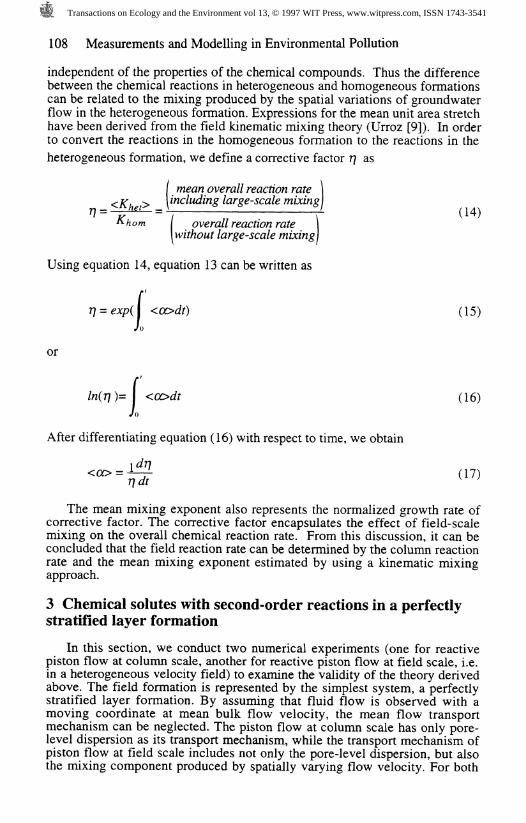
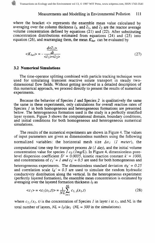
A conceptual model of the column experiment is shown in Figure 2. Thecolumn is made up of homogeneous porous media. Initially, the shadowedportion of the column is fully filled with the solution of Species 1, theremainder of the column is filled with the solution of Species 2. The chemicalreaction between Species 1 and Species 2 in this column is assumed to be asecond-order reaction that can be represented by equations (2) and (3). Thereaction shown by Figure 2 is also called a piston flow reactor.
LL
C:
Figure 2. Sketch of conceptual model for numerical experiments.
AQ in the above sketch is the area of the cross section of the column, L isthe reactor scale length which is larger than the thickness of the mixing, and, /2and Is are the horizontal and vertical widths of the column.
In this homogeneous column, without considering bulk movement of thesolute, the fate and transport of Species 1 and Species 2 through porous mediais governed by the two-dimensional equations
i= 1,3
' '
(18)
(19)
where D is the pore-scale dispersion coefficient, i = 1 represents the horizontaldirection, and / = 3 represents the vertical direction. The two governingtransport and fate equations are coupled through reaction terms because therate of the degradation for both species depends on their concentrations.
110 Measurements and Modelling in Environmental Pollution
Equations (18) and (19) describe a detailed state of solutes at every positionin the column. From an integral (reactor) point of view, the state of the columncan be also described by using the concept of the piston flow reactor. As aresult, the state of Species 1 can be described in terms of expression (7) as
-= -fAomCic: (20)
where c\ and Q are the reactor volume-averaged concentrations for Species 1and Species 2 respectively. They are defined here by
(21)Jo
and
(2%
The concentration distributions cj(x], t) and c xj, t) in equations (21) and (22)are governed by the column scale piston flow fate and transport equations (18)and (19). From equation (20), the overall reaction rate of the piston flowreactor can be estimated by
(23)C\C2
In order to explore the relationship between the reaction rates in thehomogeneous and the heterogeneous formations, heterogeneous flow alsoneeds to be investigated. The fate and transport of Species 1 and Species 2 ina heterogeneous formation can be described by
and
Arr\ r)2/*r\ rlr*-kc\ci, z=l,3 (25)
where v' is the fluctuation of velocity due to the heterogeneity of geologicformation. The overall rate equation for Species 1 in the field scale reactor wasgiven by equation (10) as
Measurements and Modelling in Environmental Pollution 111
where the bracket <> represents the ensemble mean value calculated byaveraging over the column thickness Is, and c\, and 2% are the reactor averagevolume concentration defined by equations (21) and (22). After substitutingconcentration distributions estimated from equations (24) and (25) intoequation (26), and rearranging them, the mean AT/%,, can be evaluated by
3.2 Numerical Simulations
The time-operator splitting combined with particle tracking technique wereused for simulating transient reactive solute transport in steady two-dimensional flow fields. Without getting involved in a detailed description ofthis numerical approach, we proceed directly to present the results of numericalexperiments.
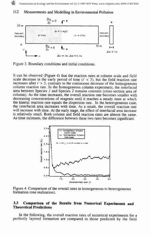
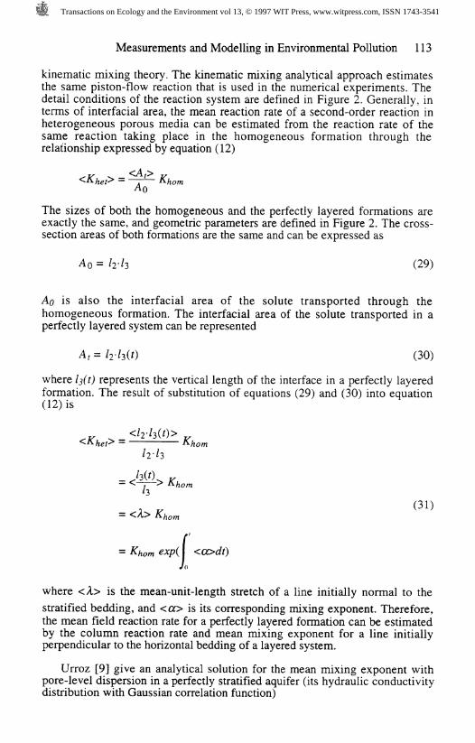
Because the behavior of Species 1 and Species 2 is qualitatively the samethe same in these experiments, only calculations for overall reaction rates ofSpecies 1 in both homogeneous and heterogeneous formations are presentedbelow. The heterogeneous formation used in the study is a perfectly stratifiedlayer system. Figure 3 shows the computational dbmain, boundary conditions,and initial conditions for both homogeneous and heterogeneous numericalsimulations.
The results of the numerical experiments are shown in Figure 4. The valuesof input parameters are given as dimensionless numbers using the following
normalized variables: the horizontal mesh size Ax/ (1 meter), the
computational time step for transport process At (1 day), and the initial volumeconcentration value for species 1 CQ (lmg/L). In Figure 4, dimensionless pore-level dispersion coefficient D' = 0.0035, kinetic reaction constant k' = 1000,and concentrations of c/' = 1 and 02 = 0.5 are used for both homogeneous and
heterogeneous experiments. The dimensionless standard deviation GK = 0.25and correlation scale IK' = 0.5 are used to simulate the random hydraulicconductivity distribution along the vertical. In the heterogeneous experiment(perfectly layered formation), the ensemble mean concentration is estimated byaveraging over the layered formation thickness Is as
NLci. X*i,0 (28)
z=l
where c/./f*/, t) is the concentration of Species 1 in layer / at.r/, andNL is the
total number of layers, ML = Is/Axj (NL = 500 in the simulations).
112 Measurements and Modelling in Environmental Pollution
-^-=0 J-a50m
free-exitboundary
s\
Co —' 1 mg/L free-exitboundary
<k^ i 30mdy *
Axi = 1m, Ax2 = 0.7m
Figure 3. Boundary conditions and initial conditions.
AX2 = / m
It can be observed (Figure 4) that the reaction rates at column scale and fieldscale decrease in the early period of time (t' < 5), but the field reaction rateincreases after t' > 5, contrary to the continuous decrease of the homogeneouscolumn reaction rate. In the homogeneous column experiment, the interfacialarea between Species 1 and Species 2 remains constant (cross-section area ofcolumn). As the time increases, the overall reaction rate becomes smaller withdecreasing concentrations of reagents until it reaches a steady state at whichthe kinetic reaction rate equals the dispersion rate. In the heterogeneous case,the interfacial area increases with time. As a result, the overall reaction ratewill increase with time. At the early stage, the effect of interfacial area increaseis relatively small. Both column and field reaction rates are almost the same.As time increases, the difference between these two rates becomes significant.
10 20 30 40Dimensionless time (t')
Figure 4. Comparison of the overall rates in homogeneous to heterogeneousformation (one realization).
3.3 Comparison of the Results from Numerical Experiments andTheoretical Predictions
In the following, the overall reaction rates of numerical experiments for aperfectly layered formation are compared to those predicted by the field
Measurements and Modelling in Environmental Pollution 113
kinematic mixing theory. The kinematic mixing analytical approach estimatesthe same piston-flow reaction that is used in the numerical experiments. Thedetail conditions of the reaction system are defined in Figure 2. Generally, interms of interfacial area, the mean reaction rate of a second-order reaction inheterogeneous porous media can be estimated from the reaction rate of thesame reaction taking place in the homogeneous formation through therelationship expressed by equation (12)
<A<Khei> =
The sizes of both the homogeneous and the perfectly layered formations areexactly the same, and geometric parameters are defined in Figure 2. The cross-section areas of both formations are the same and can be expressed as
Ao = /2'/3 (29)
AQ is also the interfacial area of the solute transported through thehomogeneous formation. The interfacial area of the solute transported in aperfectly layered system can be represented
A,= WsC) (30)
where lj(t) represents the vertical length of the interface in a perfectly layeredformation. The result of substitution of equations (29) and (30) into equation(12) is
/3
&hom
f/ng%p( I <oodf)
where <A> is the mean-unit-length stretch of a line initially normal to the
stratified bedding, and <a> is its corresponding mixing exponent. Therefore,the mean field reaction rate for a perfectly layered formation can be estimatedby the column reaction rate and mean mixing exponent for a line initiallyperpendicular to the horizontal bedding of a layered system.
Urroz [9] give an analytical solution for the mean mixing exponent withpore-level dispersion in a perfectly stratified aquifer (its hydraulic conductivitydistribution with Gaussian correlation function)
114 Measurements and Modelling in Environmental Pollution
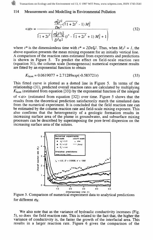
(32)
where f* is the dimensionless time with t* = 2Dl/l£. Thus, when M£ = 7, theabove equation presents the mean mixing exponent for an initially vertical line.A comparison of the reaction rates estimated from experiments and predictionsis shown in Figure 5. To predict the effect on field-scale reaction rate(equation 31), the column scale (homogeneous) numerical experiment resultsare fitted by an exponential function to obtain
= 0.0619077 + 2.71289ex/?(-0.583721f) (33)
This fitted curve is plotted as a dotted line in Figure 5. In terms of therelationship (31), predicted overall reaction rates are calculated by multiplyingKhom (estimated from equation [33]) by the exponential function of the integral
of <a> (estimated from equation [32]) over time. Figure 5 shows that theresults from the theoretical prediction satisfactorily match the simulated datafrom the numerical experiment. It is concluded that the field reaction rate canbe estimated by the column reaction rate and field-scale mixing exponent. Thisalso confirms that the heterogeneity of a geologic formation results inincreasing surface area of the plume in groundwater, and subsurface mixingprocesses can be described by superimposing the pore-level dispersion on theincreasing surface area of the solutes.
10 20 30 40 50Dimensionless time (V)
Figure 5. Comparison of numerical experiment data to analytical predictions
for different OK.
We also note that as the variance of hydraulic conductivity increases (Fig.5), so does the field reaction rate. This is related to the fact that, the higher thevariance of conductivity is, the faster the growth of the interfacial area. Thisresults in a larger reaction rate. Figure 6 gives the comparison of the
Measurements and Modelling in Environmental Pollution 115
experimental field-scale reaction rates with predicted rates for different valuesof the dimensionless correlation scale /'. The results show that as thecorrelation decreases, the field-scale reaction increases.
20 30Dimensionless time (V)
Figure 6. Comparison of the experimental field overall reaction rates topredicted field overall reaction rates for different values ofthe dimensionless correlation scale IK'.
4 Conclusions
From the presented theory and numerical results, it is apparent that theinterface behavior plays a very important role in diffusion-controlled chemicalreactions. Aquifer heterogeneities affect chemical reactions by increasing thesolute interfacial area. The field overall reaction rate can be estimated by usingthe column (homogeneous formation) reaction rate and the mean mixingexponent. The mean mixing exponent itself is determined by the spatialstructure of hydraulic conductivity of a geological formation.
5 Acknowledgments
This work was partially supported by American Petroleum Institute and theU.S. Air Force. We thank Dr. Chen Chiang of Shell Development Companyfor helpful suggestions.
References
1. Chiang, C.Y., Klein, C.L., Salanitro, J.P., and Wisniewski, H.L. Dataanalysis and computer modeling of the benzene plume in an aquiferbeneath a gas plant. Proceedings of NWWA/API Conference on PetroleumHydrocarbons and Organic Chemicals in the Ground Water, Houston,Texas, 1986.
2. Chiang, C.Y., Chai, E.Y., Salanitro, J.P., Colthart, J.D., and Klein, C.L.Effects of dissolved oxygen on the biodegradation of BTX in a sandyaquifer. Proceedings of NWWA/API Conference on Petroleum
116 Measurements and Modelling in Environmental Pollution
Hydrocarbons and Organic Chemicals in the Ground Water, Houston,Texas, 1987.
3. Kemblowski, M.W., Salanitro, J.P., Deeley, G.M., and Stanley, C.C. Fateand transport of residual hydrocarbon in groundwater - a case study.Proceedings of NWWA/API Conference on Petroleum Hydrocarbons andOrganic Chemicals in the Ground Water, Houston, Texas, 1987.
4. Hubbert, C.E., Barker, J.F., O'Hannesin, S.F., Vandegriendt, M., andGillham, R.W. Transport and fate of dissolved methanol, methyl-tertiary -butyl-ether, and monoaromatic hydrocarbons in a shallow sand aquifer.Health and Environmental Sciences Department, API Publication Number4601, American Petroleum Institute, Washington, DC., 1994.
5. Borden, R.C. Natural bioremediation of hydrocarbon-contaminatedgroundwater, in Handbook of Bioremediation, Ed. R. B. Norris, LewisPublishers, 1994.
6. Freyberg, D.L. A natural gradient experiment on solute transport in a sandaquifer 2. Spatial moments and the advection and dispersion of nonreactivetracers. Water Resour. Res., 1986, 22(13), 2031-2046.
7. Patrick, G.C., Barker, J.F., Gillham, R.W., Mayfield, C.I., and Major, D.The behavior of soluble petroleum product-derived hydrocarbons ingroundwater. Petroleum Association for the Conservation of the CanadianEnvironment, PACE Phase II Report 86-1, 1986.
8. Moltyaner, G.L., and Killey, R.W.D. Twin lake tracer tests: transversedispersion. Water Resour. Res., 198824(10), 1612-1627.
9. Urroz, G.E., Ma, Y., and Kemblowski, M.W. Advective and dispersivemixing in stratified formations. Transport in Porous Media, 1995, 18,231-243.