Estimating magnetic helicity in the Sun Kostas Moraitis LESIA, Observatoire de Paris, PSL Research University, CNRS, Sorbonne Universités, UPMC Univ. Paris 06, Univ. Paris Diderot, Sorbonne Paris Cité, 5 place Jules Janssen, 92195 Meudon, France in collaboration with M.K. Georgoulis, K. Tziotziou (RCAAM of the Academy of Athens) V. Archontis (St Andrews University), A. Nindos (University of Ioannina), ...
Transcript
Estimating magnetic helicity in the Sun
Kostas MoraitisLESIA, Observatoire de Paris, PSL Research University, CNRS, Sorbonne Universités,
UPMC Univ. Paris 06, Univ. Paris Diderot, Sorbonne Paris Cité,5 place Jules Janssen, 92195 Meudon, France
in collaboration withM.K. Georgoulis, K. Tziotziou (RCAAM of the Academy of Athens)V. Archontis (St Andrews University), A. Nindos (University of Ioannina), ...
30 Sep 2016, Meudon
Outline
● Introduction – Magnetic helicity, Free energy
● Validation of a connectivity-based method for helicity computation
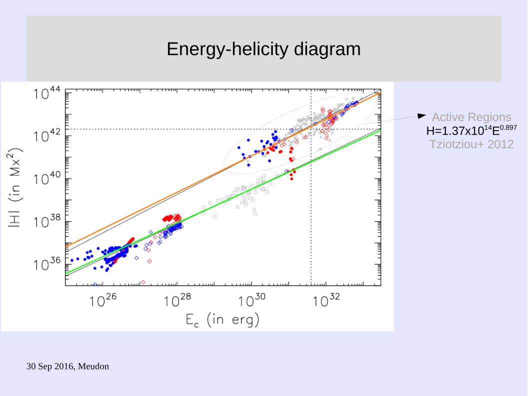
● Free energy vs helicity diagram
● Comparison of methods for the estimation of magnetic helicity
➔ A Sun-to-Earth analysis of a solar eruption
➔ In finite volumes
● Concluding remarks
30 Sep 2016, Meudon
IntroductionMagnetic helicity – Free magnetic energy
Magnetic helicity• Measure of twist and distortion of mfl• Topological invariant• Gauss linking number• Signed quantity (+ right handed, - left handed)• Splits into self + mutual terms• Helicity represents the amount of flux linkages between pairs of lines• Approximately conserved in reconnection• Emerges via helical magnetic flux tubes and/or is generated by photospheric
proper motions• An isolated configuration with accumulated magnetic helicity
cannot relax to a potential field• If not transferred to larger scales it can only be expelled bodily in
the form of CMEs
Η=∫ A⋅BdV B=∇×A
Free magnetic energy• Excess energy above potential state• Energy available for solar flares + CMEs
E c=1
8π ∫dV B2−
18π∫ dV Bp
2
30 Sep 2016, Meudon
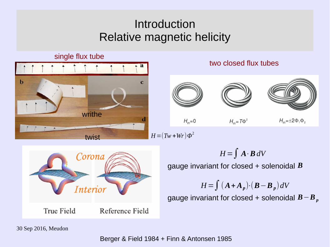
IntroductionRelative magnetic helicity
Berger & Field 1984 + Finn & Antonsen 1985
gauge invariant for closed + solenoidal B−B p
Η=∫(A+Ap)⋅(B−B p)dV
Η=∫ A⋅BdV
gauge invariant for closed + solenoidal B
two closed flux tubes
twist
writhe
single flux tube
H=(Tw +Wr )Φ2
30 Sep 2016, Meudon
Connectivity method
Steps:1. partition vector magnetogram into flux concentrations2. create connectivity matrix with flux committed to opposite polarity partitions (simulated annealing method)3. each connection=flux tube with known flux Φ, FF parameter α, position
Georgoulis & LaBonte 2007, Georgoulis+ 2012
30 Sep 2016, Meudon
Connectivity method
Steps:1. partition vector magnetogram into flux concentrations2. create connectivity matrix with flux committed to opposite polarity partitions (simulated annealing method)3. each connection=flux tube with known flux Φ, FF parameter α, position
self terms mutual terms
Georgoulis & LaBonte 2007, Georgoulis+ 2012
A, λ: constants, N: # of FTs, d: pixel size, Larch: arch number (Demoulin+ 2006)Important note: E
c budget is a lower-limit
30 Sep 2016, Meudon
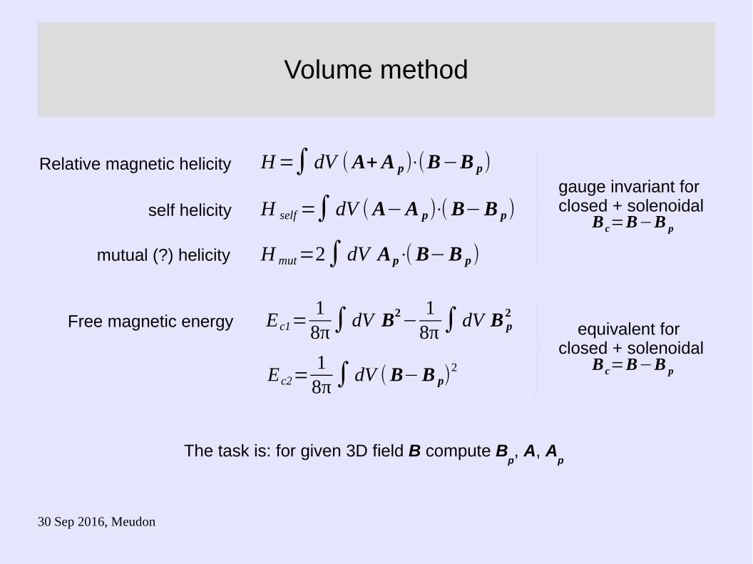
Volume method
Relative magnetic helicity
self helicity
Free magnetic energy
mutual (?) helicity
Ec2=1
8π∫ dV (B−B p)2
H=∫ dV (A+A p)⋅(B−B p)
H self=∫ dV (A−A p)⋅(B−B p)
H mut=2∫ dV Ap⋅(B−B p)
The task is: for given 3D field B compute Bp, A, A
p
E c1=1
8π∫ dV B2−
18π∫ dV B p
2
gauge invariant for closed + solenoidal
B c=B−B p
equivalent for closed + solenoidal
B c=B−B p
30 Sep 2016, Meudon
Volume method
step 1: Calculation of potential field B p=−∇ φ
with Neumann BCs
solve numerically Laplace's equation ∇2φ=0
(−∂φ/∂ n)∂V=( n⋅B)∂ V
● FISHPACK routine HW3CRT (similar to NAG routine D03FAF)● BVP well defined only for flux-balanced 3D field
(check with 2 flags)● In any case overwrite boundaries● Difference in 2 free energy expressions=measure of divergence-freeness
∮∂VB⋅d S=0
Ec 1−E c 2=−14π
∫∂Vφ(B−B p)⋅d S+
14π
∫ dV φ(∇ B c)
r=|E c 1−E c 2||Ec 1|+Ec 2
Edivg=|Ec1−Ec 2|
30 Sep 2016, Meudon
Volume method
step 2: Calculation of vector potentials A, Ap
DeVore gaugeso that
for vector potential A with the method of Valori+ 2012solve B=∇×A
z⋅A=0
A=A0− z×∫z 0
zdz ' B(x , y , z ')
A0=(−12∫y0
ydy ' B z(x , y ' , z=z0) ,
12∫x0
xdx ' B z (x ' , y , z= z0) ,0)
● Formulas valid for divergence-free fields● Differentiation with 2nd order derivatives
integration modified Simpson's rule (error 1/N4)● Top/bottom give different results - top is usually better
30 Sep 2016, Meudon
Non-eruptive synthetic AR
emergence of weakly twisted flux-tube
data: V. Archontisduration 9.5 h3 min cadence65x65x65 Mmpixel size 0.2”
30 Sep 2016, Meudon
Non-eruptive synthetic AR
r=0.72, R=0.76f=2.11±0.12
r=0.38, R=0.35f=1.96±0.21
r=0.34, R=0.29f=(8.0±1.0)x103
r=0.26, R=0.38f=1.66±0.14
30 Sep 2016, Meudon
Eruptive synthetic AR
emergence of more twisted flux-tube
data: V. Archontisduration 4.5 h3 min cadence65x65x65 Mmpixel size 0.2”
30 Sep 2016, Meudon
Eruptive synthetic AR
r=0.74, R=0.6f=2.8±0.2
r=0.6, R=0.48f=1.91±0.19
r=0.062, R=-0.007f=(7.8±1.0)x102
r=0.43, R=0.28f=0.85±0.09
30 Sep 2016, Meudon
Non-eruptive NOAA AR 11072
data: SDO/HMIextrapolation: Wiegelmann 2004(no preprocessing)20-25 May 20106 h cadence220x190x220 Mm (avg)pixel size 2”
30 Sep 2016, Meudon
Non-eruptive NOAA AR 11072
r=0.35, R=0.31f=0.45±0.25
r=0.051, R=-0.022f=0.37±0.24
r=0.11, R=0.26f=-1.0±2.1
r=-0.57, R=-0.58f=2.3±1.6
negative free energy!large E
c errors!
30 Sep 2016, Meudon
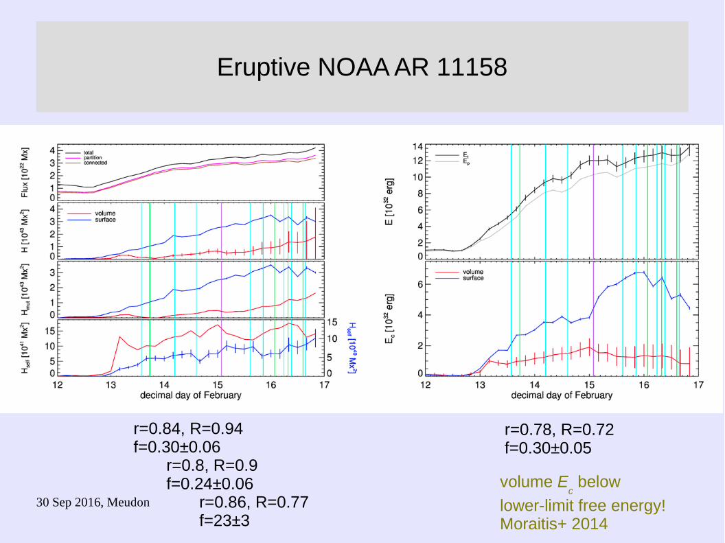
Eruptive NOAA AR 11158
X2.2 on 15 Feb 2011, 01:44 UT5 M-, tens C-class flaresdata: SDO/HMIextrapolation: Wiegelmann 2004(preprocessing, X. Sun)12-16 Feb 20114 h cadence216x216x184 Mmpixel size 1”
Origin of intense space weather phenomenaduring 7-11 March 2012 X5.4-X1.3 flares within an hour Two ultra-fast CMEs (>2000 km s-1) Interplanetary CME Major SEP event Significant ULF wave enhancements and relativistic electron dropouts in the RBs Strong energetic-electron injection in the magnetosphere - Aurorae 2nd most intense geomagnetic storm of SC24
Target of HNSWRN, Patsourakos+ 2016
Period of study: 6-7 Mar 2012 (centered on X- flares)G. Hintzoglou
NOAA AR 11429Helicity ejection
30 Sep 2016, Meudon
NOAA AR 11429CB method
From SDO/HMI magnetogramsTake LOS magnetic field components: create synthetic Stokes profiles (U, Q, V) bin them by a factor of 2 (pixel size 1”)∼ invert and obtain binned LOS magnetic field componentsResolve 180o ambiguityDe-project onto heliographic planeCoaling the derived data cubesApply free energy-helicity formulas
30 Sep 2016, Meudon
NOAA AR 11429CB method
Apparent eruption-related decrease in connected flux:reorganization of magnetic connectivity? white-light flare emission contamination?
LH helicity: decrease of 8x10∼ 42 Mx2 attributed to 1st eruption
RH helicity: increase of 2x10∼ 42 Mx2
during 1st eruptiondecrease of 2x10∼ 42 Mx2 during 2nd
Total helicity ejection 2-4x1042 Mx2
Free energy decrease of 2.5x10∼ 32 erg
Sizable errorsEruption-related changes of energy/helicityconsistent with size of eruptions
30 Sep 2016, Meudon
NOAA AR 11429FI method
From SDO/HMI sequence of vector magnetograms Disambiguated Converted to cylindrical equal area maps Compute horizontal velocities using DAVE4VM (Schuck 2008) – normal component of the ideal induction equation Removed field-aligned plasma flow Calculate G
θ
Berger & Field 1984
Pariat+ 2005Liu & Schuck 2013
Gθ( x)=−n⋅Bn(x)
2 π∫S
dS ' { x−x '
|x−x '|2 × [u(x )−u (x ') ]}Bn(x ' )
dHdt
=2∫SdS [(Ap⋅B t)vn−(Ap⋅v t)Bn ]=∫S
dS [−2(A p⋅u)Bn]
u=v t−(vn/Bn)Bt
helicity flux density
flux transport velocity
30 Sep 2016, Meudon
NOAA AR 11429FI method
Larger helicity injection before the flares than after
starting 5 March 2012 23:58 UTwith one hour cadence (Hintzoglou+ 2015)
SDO/HMI vector magnetogram data Disambiguated Converted to cylindrical equal area maps Rebin to 720 km/pixel Preprocess (Wiegelmann & Inhester 2006) Extrapolate 3D field