Introduction to Speech Processing | Ricardo Gutierrez-Osuna | CSE@TAMU 1 L9: Cepstral analysis • The cepstrum • Homomorphic filtering • The cepstrum and voicing/pitch detection • Linear prediction cepstral coefficients • Mel frequency cepstral coefficients This lecture is based on [Taylor, 2009, ch. 12; Rabiner and Schafer, 2007, ch. 5; Rabiner and Schafer, 1978, ch. 7 ]
Transcript
Introduction to Speech Processing | Ricardo Gutierrez-Osuna | CSE@TAMU 1
L9: Cepstral analysis
• The cepstrum
• Homomorphic filtering
• The cepstrum and voicing/pitch detection
• Linear prediction cepstral coefficients
• Mel frequency cepstral coefficients
This lecture is based on [Taylor, 2009, ch. 12; Rabiner and Schafer, 2007, ch. 5; Rabiner and Schafer, 1978, ch. 7 ]
Introduction to Speech Processing | Ricardo Gutierrez-Osuna | CSE@TAMU 2
The cepstrum
• Definition – The cepstrum is defined as the inverse DFT of the log magnitude of the
DFT of a signal
𝑐 𝑛 = ℱ−1 log ℱ 𝑥 𝑛
• where ℱ is the DFT and ℱ−1 is the IDFT
– For a windowed frame of speech 𝑦 𝑛 , the cepstrum is
𝑐 𝑛 = log 𝑥 𝑛 𝑒−𝑗2𝜋𝑁 𝑘𝑛
𝑁−1
𝑛=0𝑒𝑗
2𝜋𝑁 𝑘𝑛
𝑁−1
𝑛=0
DFT log IDFT 𝑥 𝑛 𝑋 𝑘 𝑋 𝑘
𝑐 𝑛
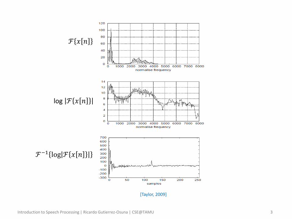
Introduction to Speech Processing | Ricardo Gutierrez-Osuna | CSE@TAMU 3
log ℱ 𝑥 𝑛
ℱ−1 log ℱ 𝑥 𝑛
ℱ 𝑥 𝑛
[Taylor, 2009]
Introduction to Speech Processing | Ricardo Gutierrez-Osuna | CSE@TAMU 4
• Motivation – Consider the magnitude spectrum ℱ 𝑥 𝑛 of the periodic signal in
the previous slide
• This spectra contains harmonics at evenly spaced intervals, whose magnitude decreases quite quickly as frequency increases
• By calculating the log spectrum, however, we can compress the dynamic range and reduce amplitude differences in the harmonics
– Now imagine we were told that the log spectra was a waveform
• In this case, we would we would describe it as quasi-periodic with some form of amplitude modulation
• To separate both components, we could then employ the DFT
• We would then expect the DFT to show
– A large spike around the “period” of the signal, and
– Some “low-frequency” components due to the amplitude modulation
• A simple filter would then allow us to separate both components (see next slide)
Introduction to Speech Processing | Ricardo Gutierrez-Osuna | CSE@TAMU 5
Liftering in the cepstral domain
[Rabiner & Schafer, 2007]
Introduction to Speech Processing | Ricardo Gutierrez-Osuna | CSE@TAMU 6
• Cepstral analysis as deconvolution – As you recall, the speech signal can be modeled as the convolution of
• Because these signals are convolved, they cannot be easily separated in the time domain
– We can however perform the separation as follows
• For convenience, we combine 𝑣′ 𝑛 = 𝑣 𝑛 ⊗ 𝑟 𝑛 , which leads to 𝑦 𝑛 = 𝑢 𝑛 ⊗ 𝑣′ 𝑛
• Taking the Fourier transform
𝑌 𝑒𝑗𝜔 = 𝑈 𝑒𝑗𝜔 𝑉′ 𝑒𝑗𝜔
• If we now take the log of the magnitude, we obtain
log 𝑌 𝑒𝑗𝜔 = log 𝑈 𝑒𝑗𝜔 + log 𝑉′ 𝑒𝑗𝜔
– which shows that source and filter are now just added together
• We can now return to the time domain through the inverse FT 𝑐 𝑛 = 𝑐𝑢 𝑛 + 𝑐𝑣 𝑛
Introduction to Speech Processing | Ricardo Gutierrez-Osuna | CSE@TAMU 7
• Where does the term “cepstrum” come from? – The crucial observation leading to the cepstrum terminology is that
the log spectrum can be treated as a waveform and subjected to further Fourier analysis
– The independent variable of the cepstrum is nominally time since it is the IDFT of a log-spectrum, but is interpreted as a frequency since we are treating the log spectrum as a waveform
– To emphasize this interchanging of domains, Bogert, Healy and Tukey (1960) coined the term cepstrum by swapping the order of the letters in the word spectrum
– Likewise, the name of the independent variable of the cepstrum is known as a quefrency, and the linear filtering operation in the previous slide is known as liftering
Introduction to Speech Processing | Ricardo Gutierrez-Osuna | CSE@TAMU 8
• Discussion – If we take the DFT of a signal and then take the inverse DFT of that, we
of course get back the original signal (assuming it is stationary)
– The cepstrum calculation is different in two ways
• First, we only use magnitude information, and throw away the phase
• Second, we take the IDFT of the log-magnitude which is already very different since the log operation emphasizes the “periodicity” of the harmonics
– The cepstrum is useful because it separates source and filter
• If we are interested in the glottal excitation, we keep the high coefficients
• If we are interested in the vocal tract, we keep the low coefficients
• Truncating the cepstrum at different quefrency values allows us to preserve different amounts of spectral detail (see next slide)
Introduction to Speech Processing | Ricardo Gutierrez-Osuna | CSE@TAMU 9
[Taylor, 2009]
K=10
K=20
K=30
K=50
Frequency (Hz)
Introduction to Speech Processing | Ricardo Gutierrez-Osuna | CSE@TAMU 10
– Note from the previous slide that cepstral coefficients are a very compact representation of the spectral envelope
– It also turns out that cepstral coefficients are (to a large extent) uncorrelated
• This is very useful for statistical modeling because we only need to store their mean and variances but not their covariances
– For these reasons, cepstral coefficients are widely used in speech recognition, generally combined with a perceptual auditory scale, as we see next
Introduction to Speech Processing | Ricardo Gutierrez-Osuna | CSE@TAMU 11
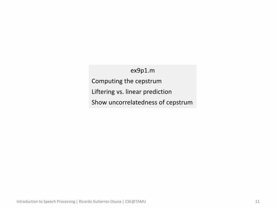
ex9p1.m
Computing the cepstrum
Liftering vs. linear prediction
Show uncorrelatedness of cepstrum
Introduction to Speech Processing | Ricardo Gutierrez-Osuna | CSE@TAMU 12
Homomorphic filtering
• Cepstral analysis is a special case of homomorphic filtering – Homomorphic filtering is a generalized technique involving (1) a
nonlinear mapping to a different domain where (2) linear filters are applied, followed by (3) mapping back to the original domain
– Consider the transformation defined by 𝑦 𝑛 = 𝐿 𝑥 𝑛
• If 𝐿 is a linear system, it will satisfy the principle of superposition 𝐿 𝑥1 𝑛 + 𝑥2 𝑛 = 𝐿 𝑥1 𝑛 + 𝐿 𝑥2 𝑛
– By analogy, we define a class of systems that obey a generalized principle of superposition where addition is replaced by convolution
𝐻 𝑥 𝑛 = 𝐻 𝑥1 𝑛 ∗ 𝑥2 𝑛 = 𝐻 𝑥1 𝑛 ∗ 𝐻 𝑥2 𝑛
• Systems having this property are known as homomorphic systems for convolution, and can be depicted as shown below
[Rabiner & Schafer, 1978]
Introduction to Speech Processing | Ricardo Gutierrez-Osuna | CSE@TAMU 13
– An important property of homomorphic systems is that they can be represented as a cascade of three homomorphic systems
• The first system takes inputs combined by convolution and transforms them into an additive combination of the corresponding outputs
– Thus, the frequency domain representation of a homomorphic system for deconvolution can be represented as
[Rabiner & Schafer, 1978]
Introduction to Speech Processing | Ricardo Gutierrez-Osuna | CSE@TAMU 15
– If we wish to represent signals as sequence rather than in the frequency domain, then the systems 𝐷∗ and 𝐷∗
−1 can be represented as shown below
• Where you can recognize the similarity between the cepstrum with the system 𝐷∗
• Strictly speaking, 𝐷∗ defines a complex cepstrum, whereas in speech processing we generally use the real cepstrum
– Can you find the equivalent system for the liftering stage?
[Rabiner & Schafer, 1978]
Introduction to Speech Processing | Ricardo Gutierrez-Osuna | CSE@TAMU 16
Voicing/pitch detection
• Cepstral analysis can be applied to detect local periodicity – The figure in the next slide shows the STFT and corresponding spectra
for a sequence of analysis windows in a speech signal (50-ms window, 12.5-ms shift)
– The STFT shows a clear difference in harmonic structure
• Frames 1-5 correspond to unvoiced speech
• Frames 8-15 correspond to voiced speech
• Frames 6-7 contain a mixture of voiced and unvoiced excitation
– These differences are perhaps more apparent in the cepstrum, which shows a strong peak at a quefrency of about 11-12 ms for frames 8-15
– Therefore, presence of a strong peak (in the 3-20 ms range) is a very strong indication that the speech segment is voiced
• Lack of a peak, however, is not an indication of unvoiced speech since the strength or existence of a peak depends on various factors, i.e., length of the analysis window
Introduction to Speech Processing | Ricardo Gutierrez-Osuna | CSE@TAMU 17
[Rabiner & Schafer, 2007]
Introduction to Speech Processing | Ricardo Gutierrez-Osuna | CSE@TAMU 18
Cepstral-based parameterizations
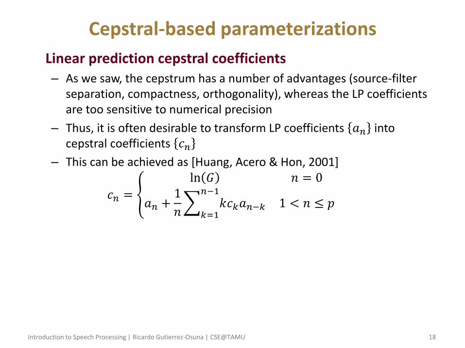
• Linear prediction cepstral coefficients – As we saw, the cepstrum has a number of advantages (source-filter
separation, compactness, orthogonality), whereas the LP coefficients are too sensitive to numerical precision
– Thus, it is often desirable to transform LP coefficients 𝑎𝑛 into cepstral coefficients 𝑐𝑛
– This can be achieved as [Huang, Acero & Hon, 2001]
𝑐𝑛 =
ln 𝐺 𝑛 = 0
𝑎𝑛 +1
𝑛 𝑘𝑐𝑘𝑎𝑛−𝑘
𝑛−1
𝑘=11 < 𝑛 ≤ 𝑝
Introduction to Speech Processing | Ricardo Gutierrez-Osuna | CSE@TAMU 19
• Mel Frequency Cepstral Coefficients (MFCC) – Probably the most common parameterization in speech recognition
– Combines the advantages of the cepstrum with a frequency scale based on critical bands
• Computing MFCCs – First, the speech signal is analyzed with the STFT
– Then, DFT values are grouped together in critical bands and weighted according to the triangular weighting function shown below
• These bandwidths are constant for center frequencies below 1KHz and increase exponentially up to half the sampling rate
[Rabiner & Schafer, 2007]
Introduction to Speech Processing | Ricardo Gutierrez-Osuna | CSE@TAMU 20
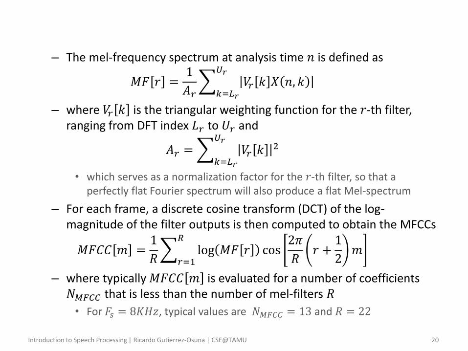
– The mel-frequency spectrum at analysis time 𝑛 is defined as
𝑀𝐹 𝑟 =1
𝐴𝑟 𝑉𝑟 𝑘 𝑋 𝑛, 𝑘
𝑈𝑟
𝑘=𝐿𝑟
– where 𝑉𝑟 𝑘 is the triangular weighting function for the 𝑟-th filter, ranging from DFT index 𝐿𝑟 to 𝑈𝑟 and
𝐴𝑟 = 𝑉𝑟 𝑘2
𝑈𝑟
𝑘=𝐿𝑟
• which serves as a normalization factor for the 𝑟-th filter, so that a perfectly flat Fourier spectrum will also produce a flat Mel-spectrum
– For each frame, a discrete cosine transform (DCT) of the log-magnitude of the filter outputs is then computed to obtain the MFCCs
𝑀𝐹𝐶𝐶 𝑚 =1
𝑅 log 𝑀𝐹 𝑟 cos
2𝜋
𝑅𝑟 +
1
2𝑚
𝑅
𝑟=1
– where typically 𝑀𝐹𝐶𝐶 𝑚 is evaluated for a number of coefficients 𝑁𝑀𝐹𝐶𝐶 that is less than the number of mel-filters 𝑅
• For 𝐹𝑠 = 8𝐾𝐻𝑧, typical values are 𝑁𝑀𝐹𝐶𝐶 = 13 and 𝑅 = 22
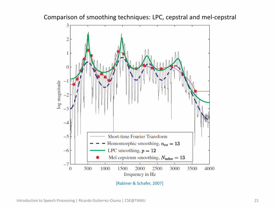
Introduction to Speech Processing | Ricardo Gutierrez-Osuna | CSE@TAMU 21
[Rabiner & Schafer, 2007]
Comparison of smoothing techniques: LPC, cepstral and mel-cepstral
Introduction to Speech Processing | Ricardo Gutierrez-Osuna | CSE@TAMU 22
• Notes – The MFCC is no longer a homomorphic transformation
• It would be if the order of summation and logarithms were reversed, in other words if we computed
1
𝐴𝑟 log 𝑉𝑟 𝑘 𝑋 𝑛, 𝑘
𝑈𝑟
𝑘=𝐿𝑟
• Instead of
log1
𝐴𝑟 𝑉𝑟 𝑘 𝑋 𝑛, 𝑘
𝑈𝑟
𝑘=𝐿𝑟
• In practice, however, the MFCC representation is approximately homomorphic for filters that have a smooth transfer function
• The advantages of the second summation above is that the filter energies are more robust to noise and spectral properties
Introduction to Speech Processing | Ricardo Gutierrez-Osuna | CSE@TAMU 23
– MFCCs employ the DCT instead of the IDFT
• The DCT turns out to be closely related to the Karhunen-Loeve transform
– The KL transform is the basis for PCA, a technique that can be used to find orthogonal (uncorrelated) projections of high dimensional data
– As a result, the DCT tends to decorrelate the mel-scale frequency log-energies
• Relationship with the DFT
– The DCT transform (the DCT-II, to be exact) is defined as
𝑋𝐷𝐶𝑇 𝑘 = 𝑥 𝑛 cos𝜋
𝑁𝑛 +
1
2𝑘
𝑁−1
𝑛=0
– whereas the DFT is defined as
𝑋𝐷𝐹𝑇 𝑘 = 𝑥 𝑛 𝑒𝑗2𝜋𝑁 𝑘𝑛
𝑁−1
𝑛=0
– Under some conditions, the DFT and the DCT-II are exactly equivalent
– For our purposes, you can think of the DCT as a “real” version of the DFT (i.e., no imaginary part) that also has a better energy compaction properties than the DFT
Introduction to Speech Processing | Ricardo Gutierrez-Osuna | CSE@TAMU 24