Labor Supply Along the Extensive and Intensive Margin...

Labor Supply Along the Extensive and Intensive Margin:

Cross-Country Facts and Time Trends by Gender

Alexander BickArizona State University

Bettina BruggemannGoethe University Frankfurt

Nicola Fuchs-SchundelnGoethe University Frankfurt, CEPR and CFS

March 27, 2014

VERY PRELIMINARY; PLEASE DO NOT QUOTE

Abstract

This paper documents facts about labor supply along the extensive and intensive margin forvarious demographic subgroups in the US and 18 European countries for the time period 1983 to2011. To do this, we recur to three different micro data sets, describe in detail how to make thedata sets consistent internationally and over time, and compare them to aggregate data fromthe OECD and the Conference Board. In a recent pre-crisis cross-section, gender differencesin hours worked are largest in Western and Southern Europe, driven mostly by the intensivemargin in Western Europe and the extensive margin in Southern Europe. Employment rateshave consistently been increasing for women in the last three decades, while the picture forhours worked per employed is more diverse. A very strong stylized fact is a negative correlationof employment rates and hours worked per employed for women in the recent cross-section,over time, and for all demographic subgroups. We present some suggestive evidence that thisnegative correlation is at least partly driven by a lack of part-time jobs in Eastern and SouthernEurope, and that increases in flexibility can raise female labor market attachment. Last, wedocument that male hours worked declined more than female hours worked in the recent GreatRecession, both along the extensive and along the intensive margin, but that this is an artefactof sectoral and educational effects for the extensive margin.

1 Introduction

An active recent literature has documented large differences in the levels and trends of aggregate

labor supply across OECD countries. The literature traces these back to, among others, labor

income taxation (Prescott (2004), Rogerson (2006), Rogerson (2008), Rogerson (2009), Ohanian

et al. (2008), McDaniel (2011)), institutions (Alesina et al. (2005)), and social security systems

(Wallenius (2013)).

To better understand the causes of the large differences in labor supply, it is useful to know

whether these differences exist uniformly in the population, or are instead driven by specific de-

mographic subgroups. In order to answer this question, one needs micro data to document hours

worked by demographic characteristics. In this paper, we use the European Labor Force Survey,

the US Current Population Survey, and the German Microcensus to document differences in labor

supply across 19 OECD countries along the extensive and intensive margin by gender, also analyz-

ing other characteristics like marital status, the presence of children, education, and sectors. In the

first part of the paper, we describe in detail how we calculate annual hours worked from the micro

data sets, and compare annual aggregate hours worked per employed and employment rates in our

data to comparable data series from the OECD and the Conference Board. The second part of the

paper then documents several facts on labor supply along the extensive and the intensive margin

for different demographic subgroups in a recent pre-crisis cross-section, over time, and during the

Great Recession.

We construct annual hours worked per person by multiplying aggregate employment rates and

hours worked per employed. To get the former from the micro data sets, we rely on the self-

reported employment status of individuals. To obtain the latter, we construct individual annual

hours from actual weekly hours worked in a reference week. Since reference weeks are not spread

continuously over the year, and since we find additional evidence for underreporting of vacation

days and public holidays, we collect these from external data sources to control for them directly.

We report international differences in self-reported and official vacation days and public holidays,

as well as in other reasons for hours lost, such as sickness and maternity leave. To maximize

the international comparability of the data, we employ a common capping across countries, and

document the potential effects of this capping. Last, we compare our data to data from the OECD

and the Conference Board in both levels and trends. The micro data sets report on average higher

employment rates than the OECD, while the picture for hours worked per employed is somewhat

mixed. For Germany and the US, we investigate further potential reasons for the differences in

hours worked per employed in the micro data and as provided by the OECD, and present some

evidence that in fact the OECD underestimates hours worked per employed, while the micro data

sets might give more reliable information. We do not find any significant correlation between under-

or overestimation of hours worked per employed and different data sources by the OECD, which

relies on either national accounts, establishment surveys, labor force surveys, or mixed sources.

1

Time trends in the micro data line up well with trends in OECD or Conference Board data.

When we present hours worked facts, we focus on individuals aged 15 to 64, and on differences

by gender. In a recent pre-crisis cross-section of the years 2003-2007, we show that hours worked

per person are substantially higher in the US than in Europe, but surprisingly homogeneous within

Europe. This homogeneity masks however substantial heterogeneity along two lines: first, by

gender, with female hours lagging substantially behind male hours, and the gender hours gap being

largest in Western and Southern Europe; and secondly, along the extensive and the intensive margin,

with countries in Scandinavia and Western Europe exhibiting high employment rates and low hours

worked per employed, while the opposite is true in Eastern and Southern Europe. For women, we

document a strong negative cross-country correlation between employment rates and hours worked

per employed, which is present for all demographic subgroups by marital status and presence of

children. The largest difference between Europe and the US arises for unmarried women with

school children, which work around 700 hours more in the US than in Europe, mostly driven by a

stronger labor market attachment arising after the Clinton welfare reforms of the 1990s. Part-time

work rates, defined as the percentage of employed women working less than 30 usual hours weekly,

are around 40 percent in Western Europe and Scandinavia, but substantially lower in the other

regions. We present some suggestive evidence that part-time jobs are in scarce supply in Eastern

and Southern Europe, forcing women there to adjust their hours along the extensive margin. The

negative correlation between female employment rates and hours worked per employed also arises

in time trends since the 1980s, but becomes somewhat weaker in the last decade. An increase in

female labor market participation can be observed in all countries, with an increasing convergence

in the last decade, while hours worked per employed developments show more heterogeneity.

Last, we document hours worked during the Great Recession. A striking pattern is that on

average across all countries male employment rates and hours worked per employed fell substantially

more than female ones. For the employment rate, this is however not driven by an underlying gender

effect, but by the different sectoral and educational composition of the male and female work force,

as well as by different pre-crisis trends by gender. For hours worked per employed, we still observe a

significantly larger decline for men than for women after controlling for many confounding factors.

The gender difference of the decline is largest for the low educated. This could indicate an inability

of employers to cut back hours worked of women, who often work part-time.

The remainder of the paper is structured as follows: Section 2 describes the micro data sets.

The following section explains how we calculate individual annual hours worked from a measure

of weekly actual hours worked. Section 4 then explains the construction of aggregate measures of

hours worked, analyzes the effect of using external data to account for public holidays and vacation

days, and compares aggregate hours worked per employed and employment rates from our data to

those reported by the OECD and the Conference Board. The next three sections document hours

worked along the extensive and intensive margin for men and women. Section 5 describes facts

2

from a recent pre-crisis cross-section (2003-2007), while Section 6 looks at trends over the last three

decades, starting in 1983. Section 7 then documents the development of employment rates and

hours worked per employed by gender in the Great Recession. Finally, Section 8 concludes.

2 Data Sets

We work with three different micro data sets to construct hours worked, namely the European

Labor Force Survey, the Current Population Survey, and the German Microcensus.

2.1 European Labor Force Survey

The European Labor Force Survey (ELFS) is a collection of annual labor force surveys from different

European countries, with the explicit goal to make them comparable across countries. We use the

yearly surveys, since the quarterly ones do not provide information on marital status and education.

The ELFS covers Belgium, Denmark, France, Greece, Italy, Ireland, the Netherlands,1 and the UK

from 1983 on, Portugal and Spain starting in 1986, Austria, Norway, and Sweden starting in 1995,

Hungary and Switzerland starting in 1996, and the Czech Republic and Poland starting in 1997.2

The sample size of the ELFS varies across countries and also within a country over time, but is

always of considerable magnitude.

2.2 Current Population Survey

For the US, we use the Current Population Survey (CPS), which is a monthly survey of around

60,000 households. Specifically, we work with the CPS Merged Outgoing Rotation Groups data pro-

vided by the National Bureau of Economic Research (see http://www.nber.org/data/morg.html).

This data set includes only those interviews in which the households are asked about actual and

usual hours worked, namely the fourth and eighth interview of every household. The data covers

around 300,000 individuals per year.

2.3 German Microcensus

The German Microcensus covers a one percent random sample of the population of Germany and

is an administrative survey. Participation is mandatory. We use the scientific use files, which are a

70 percent random subsample of the original sample. This leaves us with a sample size of between

400,000 and 500,000 individuals per year. The scientific use files are available biannually from 1985

1For the Netherlands, we have information from 1983, 1985, and annually from 1987 on.2The ELFS also covers Finland from 1995 on. However, the Finish data have large numbers of missing observations

for several years, which implies that we could only use data from 1997 to 2002 for our analysis. We therefore excludeFinland entirely from the analysis. The ELFS covers also covers more transition countries, which we however excludefrom the analysis because of data limitations along several dimensions.

3

on, and annually from 1995 on. East Germans are included in the sample from 1991 onwards.3

The German Microcensus groups hours together if the number of observations per indicated hours

worked becomes too small. This mostly concerns high numbers of hours worked, and mostly groups

two adjacent hours together. In this case, we always take the mid value as the hours worked.4

3 Calculation of Annual Hours Worked per Person

3.1 Key Variables

The calculation of annual hours worked is based on four variables from the micro data sets, namely

usual hours worked in the main job in a working week, actual hours worked in the main job in

the reference week, actual hours worked in additional jobs in the reference week, and reasons for

having worked more or less hours than usual in the reference week.

3.2 Capping

In the ELFS, the largest possible value for usual or actual hours worked per week in the main

job is 80, with the possibility of another maximum of 80 actual hours of work in additional jobs.

In the CPS, the largest possible value for actual hours worked in all jobs is 99 hours per week.

We harmonize the different capping procedures implemented by ELFS and CPS by introducing a

common cap. To achieve maximum consistency across countries, we cap the possible number of

actual and usual hours worked per week in all jobs at 80.

Even though we have not yet introduced how we construct annual hours worked, we can reassure

the reader that capping total hours at 80 hardly makes a difference for the amount of average

annual hours worked per employed, see Table A.1 in Appendix A.1. For the European countries,

the difference between capped and uncapped hours worked per employed only exceeds 0.1% in one

case (Norway, where it amounts to 0.11%) and only 0.07% of observations are affected on average.

Capping US hours worked reduces annual hours per employed slightly more, with an average of

0.19%. As a caveat, the table only shows the effect of the additional capping that we implement;

we cannot gauge the size of the effect of the initial capping implemented by the surveys, but it is

likely to be very small. The fraction of observations at the highest allowed value for hours actually

worked in the main job is 0.7% for the ELFS, 0.2% for the CPS and 0.03% for the Microcensus.

3From 2002 on, data from the German Microcensus are used also as input into the European Labor Force Survey,but before 2002 Germany is missing from the anonymized ELFS available to researchers.

4When instead using the maximum values in each grouping, the resulting difference in average annual hours workedper person amounts to only 0.02%.

4

3.3 Treatment of Missing Values

We drop some observations from the sample due to missing values. If actual hours are missing,

we replace them by zero if the respondent indicates not having worked in the reference week. If

the respondent states that he/she has been working in the reference week, but actual hours are

missing, we drop the observation. Observations with missing usual hours are only dropped when we

need usual hours, see the next subsection for further details. Table A.2 in Appendix A.1 shows the

percentage of observations dropped due to the different reasons. With the exceptions of Belgium

and Switzerland, the percentages are far below 1 percent.

3.4 From Weekly to Annual Hours Worked per Person

We build two different measures of annual hours worked on the individual level. First, we add up

actual weekly hours worked in the reference week for all jobs, and then multiply by 52. We call the

resulting measure of annual hours worked “Raw Micro Data”. This measure should be suitable for

calculating average annual hours worked per person if the reference weeks were evenly distributed

over the entire year. However, as the following subsection explains, this is not the case, and thus

further adjustments are necessary, which we offer in our second measure “Adjusted Micro Data”.

3.5 The Distribution of Reference Weeks

The reference week referred to in labor force surveys is mostly the week preceding the interview

week. If reference weeks are not spread evenly over the year, then one might systematically over-

or underestimate annual hours worked due to under- over overrepresentation of public holidays or

vacation days in the sampled weeks.

To give a concrete example, the CPS covers all 12 months of the year, but uses as a reference

week always the week into which the 12th of the month falls. Therefore, most major US public

holidays, which often lie at the beginning or the end of the month, are not captured by the CPS

(e.g. 4th of July, Thanksgiving, Memorial Day). The German Microcensus used one single reference

week, which fell into the end of April or beginning of May and deliberately excluded weeks with a

public holiday, until 2004, and from 2005 on covers the entire year.

The reference weeks in the national labor force surveys of the European countries initially fell

only into specific periods, but all surveys (with the exception of the Irish one) switched to an even

spread of reference weeks over the entire year at some point in time, albeit in different years. There

are considerable differences in the number of weeks that were covered before continuous surveying

emerged, ranging from one single reference week to the coverage of half a year. Eurostat, in its

efforts to harmonize the different surveys as much as possible, treated the changes in reference

weeks in a two-step procedure. First, when the actual change to continuous surveying occurred

in different years for the different countries, the ELFS micro data reflects this by changing from

5

covering only single weeks to covering the second quarter of the calendar year (April to June) from

then on, with some exceptions to this rule (detailed in Web Appendix W.1). In a second step in

2005, when the majority of countries included in the ELFS had changed to continuous surveying,

the ELFS micro data switched to covering the entire 52 weeks of the year for all countries that had

adapted continuous surveying. The only exceptions to this second step rule are the UK (continuous

surveying from 2008 on), Switzerland (from 2010 on), and Ireland, where the switch has not yet

taken place.

Table W.1 in Web Appendix W.1 reflects the distribution of reference weeks for the ELFS

countries at three different points in time: The year before the actual change to continuous surveying

took place, the year of that change, and the year in which the actual change was implemented into

the ELFS micro data (2005 in most countries). The appendix also discusses exceptions to the

two-step procedure of implementing continuous surveying by Eurostat described above.

3.6 Supplementation through External Data Sources

In order to account for any bias introduced by the lack of representativeness of the reference weeks,

we introduce a second measure of annual hours worked which incorporates data from external

sources, following a procedure suggested by the OECD, see Pilat (2003).

For the construction of our second hours measure “Adjusted Micro Data” we proceed as follows,

starting with weekly hours worked. As a baseline, we calculate weekly hours worked as actual

hours worked in the reference week in the main job and all additional jobs. However, if respondents

indicate that they worked less hours than usual in the main job in the reference week because of

public holidays and/or annual leave, we replace actual weekly hours by usual weekly hours in the

main job plus actual weekly hours worked in additional jobs.5

We then use external data sources to account for average lost working time because of public

holidays and days of annual leave. This is done by calculating an adjusted measure of weeks

worked per year, weeksadj = 52 − daleave+dpubhol5 , where daleave are average days of annual leave,

and dpubhol is the sum of public holidays. We then calculate individual annual hours worked by

multiplying weekly hours by this adjusted number of weeks. The resulting measure is denoted

“Adjusted Micro Data”. Note that a disadvantage of this procedure is that we cannot account for

heterogeneity across the population in terms of days of annual leave and public holidays, and have

to assume that these days are actually taken by every employed person, an assumption on which

we report some evidence in Section 4.2.6

5For additional jobs, we don’t have information on usual hours. If respondents state that they have been workingless hours than in a usual week because of public holidays or annual leave, but usual hours in the main job aremissing, these observations are dropped.

6In Appendix A.1 we discuss some differences between the CPS and ELFS questionnaire regarding the constructionof the hours measure “Adjusted Micro Data”, which however have virtually no impact on the statistics presented inthe paper.

6

Figure 1: Public holidays and days of annual leave from external data sources (all available years)

010

20

30

40

DE IT FR AT SE ES PT CZ NO DK GR CH BE UK PL IE NL HU US

Public holidays Days of annual leave

For some countries (Denmark, France, Germany, Netherlands, Switzerland, United Kingdom,

United States), we obtain statistics on average numbers of public holidays and days of annual leave

covering the entire sample period from the national statistical offices and other public institutions,

detailed in Appendix A.2. For the remaining countries, average days of annual leave and public

holidays are obtained from the European Industrial Relations Observatory (EIRO), which provides

data on days of annual leave and public holidays for the years 2002 to 2011. For the years prior

to 2002, we use two different strategies. For some countries (Austria, Belgium, Portugal, and

Sweden), we were able to obtain from the International Labor Organization ILO the number of

days of national bank holidays (subtracting those falling on a Sunday) as well as the number of days

of annual leave, both as indicated by national laws (i.e. ILO refers to labor laws rather than actual

collected statistics as sources of these numbers). For the remaining countries (Czech Republic,

Greece, Hungary, Ireland, Italy, Norway, Poland, and Spain), we use the EIRO mean over the years

2002 to 2011 to extend the series backwards.

Figure 1 shows the average number of public holidays and days of annual leave for the countries

in our sample. The cross-country variation in annual leave days is substantially larger than the

cross-country variation in public holidays. The sum of both varies between more than 40 days in

Germany and less than 20 days in the US.

Table A.5 in Appendix A.2 details the average number of public holidays and annual leave

days at the beginning and the end of the sample period for the different countries. While there is

7

some time series variation, it is small, namely less than a day, for the majority of countries, with

the notable exception of Denmark, where public holidays plus days of annual leave increased by

almost 7 days between 1983 and 2011. The Web Appendix W.2 contains detailed graphs displaying

the annual numbers of public holidays and annual leave days for all countries, in addition to a

comparison to the EIRO data for the group of countries for which we have data from both national

statistical offices and EIRO.

Note that if sick leave days exhibit a seasonal pattern, an uneven distribution of reference weeks

over the year also leads to systematic under- or overrepresentation of sick days. Since we do not

have reliable external data on sick leave days for a large number of country/year observations, we

cannot control for this potential bias using external data sources. However, Section A.3 shows some

suggestive evidence that the seasonality of sick days is not a large problem for our surveys, since

the number of sick days does not change much for most countries as they switch from surveying

only specific weeks to continuous surveying.

3.7 Dropping Specific Country/Year Observations

There are a number of country/year observations that have been dropped in the calculation of

averages due to different inconsistencies and particularities. Specifically, we exclude the years 1983

for Denmark, 2001 for the UK, and 2005 for Spain from our analysis. The Danish data for 1983

suggest that only around 23 percent of all observed individuals were employed, which is around one

third of the employment rate that we observe in other years. In the UK in 2001, 3.2 percent of the

respondents report not having worked at all in the reference week despite having a job due to bad

weather (“other” reasons), compared to around 0.03 percent before and after 2001. By contrast, in

2001 only 0.32 percent report not having worked in the reference week despite having a job due to

annual leave, compared to more than 3 percent in 2000 and 2002. This suggests that the categories

have been switched accidentally, but since we cannot be certain, we do not include 2001 into our

analysis. For Spain, 3.4 percent of the respondents report having worked less than usual due to

compensation leave in 2005, compared to less than 0.03 percent in 2004 and 2006. Average hours

lost due to “other” reasons are seven times larger in 2005 than in the previous and subsequent

years (2.8 as opposed to 0.4), which ultimately leads to a large drop in hours worked in 2005.

Table A.3 in Appendix A.1 gives the final total sample size of individuals aged 15-64, for each

country/year combination. The annual sample size per country ranges from 10,000 to 450,000 with

an average of 115,000 observations.

8

4 Aggregate Measures of Labor Supply

4.1 Construction of Average Hours Worked per Person

We construct average annual hours worked per person HWP by first calculating average hours

worked per employed, HWE, and then multiplying by the employment rate, ER, such that

HWP = ER ·HWE. The employment rate is based on the self-reported employment status ei of

the individual and also includes self-employed (with or without employees) and family workers.7

Formally, ER = Ne

N with N being the sample size and N e=∑N

i=1 ei.

For calculating average hours worked per employed, we calculate the sum of annual hours worked

of all individuals who self-report being employed, and then divide by the number of employed

individuals.8 Thus, if hi are annual hours worked of individual i, then HWE = 1Ne

∑Ni=1 hi ∗ ei.

Therefore, an individual who is employed but reports zero hours worked in the reference week,

e.g. due to sickness, will contribute zero hours to the hours worked per employed. In all these

calculations, we only incorporate information from individuals between the ages of 15 and 64. When

we look at specific demographic subgroups, the overall population refers to number of observations

in this subgroup. Every observation is weighted by the weights provided in the different surveys.

4.2 Comparison of the Raw and the Adjusted Micro Data

We now have two measures of average annual hours worked: the Raw Micro Data only uses informa-

tion from the labor force surveys, whereas the Adjusted Micro Data uses external data to account

for the fact that reference weeks are not spread out continuously over the year in most countries

before 2005, with the consequence that public holidays and days of annual leave are misrepresented

in the micro data. With the shift to continuous surveying, this concern should evaporate and the

Raw and Adjusted Micro Data should in principle yield similar values.

Figure 2 shows the average percentage deviation of the Raw Micro Data from the Adjusted Micro

Data for each country for (up to) three different periods: the years before continuous surveying was

introduced (“specific weeks”), the years for which continuous surveying was carried out, but only

implemented in the ELFS in a first step by introducing the second quarter data (“2nd quarter”),

and the years in which ELFS data in fact covers the entire year (“continuous”). For some countries,

not all three definitions apply.

Since public holidays and annual leave days are underrepresented before continuous surveying

over the entire year is introduced, the Adjusted Micro Data always reports lower hours than the

Raw Micro Data. The difference is significant, ranging between 3.5 and 17 percent.9 Covering the

second quarter mostly leads to a decrease in the difference between the Adjusted Micro Data and

7ei is a dummy variable taking the value 1 if the individual reports being employed, and 0 otherwise. Section W.3in the Web Appendix reports alternative measures of employment.

8Non-employed individuals are not asked about their hours worked, which are zero by definition.9The difference is largest for Germany, which until 2004 used only one single week as reference week.

9

Figure 2: %-Deviations of hours worked per employed of the Raw and the Adjusted Micro Data

−1

13

57

911

13

15

17

AT BE CH CZ DE DK ES FR GR HU IE IT NL NO PL PT SE UK US

Specific Weeks 2nd Quarter Continuous

the Raw Micro Data, and going to continuous surveying to a further decrease in all countries but

Denmark and the UK.10

However, while for some countries, e.g. the Netherlands or Sweden, differences between the

Adjusted the Raw Micro Data almost disappear after continuous surveying is introduced (“after”),

for some countries they remain important: in 9 of the 19 countries, the Raw Micro Data still reports

more than 5 percent higher hours than the Adjusted Micro Data even when the reference weeks

cover the entire year. The discrepancy is largest for Germany, where it amounts to more than 11

percent, and is generally larger in Southern and Eastern Europe than in Scandinavia and Western

Europe. This indicates a discrepancy between the numbers of public holidays and annual leave

days indicated in the micro data and given in national statistics, where in every case the former is

lower than the latter. One reason for this is that even if all weeks are covered by the surveys, they

are not always covered evenly.

To further investigate why differences between the Raw and Adjusted Micro Data are still

prevalent after introduction of continuous surveying, we compare in the first two columns of Table

1 weeks lost due to vacation/public holidays based on self-reports in the micro data to vacation

10Figures W.20 to W.38 in Web Appendix W.4 show the time series comparisons between the Raw and the AdjustedMicro Data for each country. In each figure, the solid vertical line indicates the year in which the first-step of thechange to continuous surveying was implemented in the ELFS (mostly resulting in a wider spread of the referenceweek), while the dashed vertical line indicates the first year in which the micro data available to the researcheractually cover the entire year.

10

days and public holidays from external data for the year 2006. For the self-reports, we build the

difference between actual and usual hours worked in the main job as a percentage of usual hours

worked if an individual reports having worked less than usual due to vacation or public holidays,

and then multiply by 52.11 The differences are very large, often amounting to more than 3 weeks. In

6 of the 19 countries, self-reported public holidays and vacation days amount to less than 2 weeks.

Overall, given that public holidays alone in many countries sum up to 1.5 weeks, the self-reported

number of the sum of vacation days and public holidays seems too small. In some countries, this

is driven by the fact that a small number of the population reports working less hours than usual

in the reference week due to holidays and vacation days (see column 3 of Table 1), which might

indicate that respondents do not use the correct week as reference week when in fact vacation days

and public holidays fell into the reference week (this might e.g. be due to the fact that they think it

is more appropriate to report hours of a “typical” work week). Appendix A.3 shows the distribution

of further reasons for working less hours than usually in the reference week by country.

To understand these discrepancies better, we further analyze the case of Germany as an ex-

emplary country. External data reports 8.3 weeks of vacation days and public holidays, while

Microcensus self-reports add up to on average 2.4 weeks, creating a large discrepancy of 5.9 weeks,

the largest one of all countries. The external data for Germany come from the IAB (for a detailed

description, see Wanger 2013). The IAB calculates vacation days based on agreed vacation days

in official labor contract negotiations. They take into account differences across sectors as well

as age groups, creating a weighted average.12 Schnitzlein (2011) reports based on data from the

German Socio-Economic Panel that on average 3 agreed vacation days per year go unused. Thus,

the underusage of vacation days can probably explain only a very small portion of the discrepancy

of 5.9 weeks between self-reports and official vacation days.

Analyzing the Microcensus data further, there could be several reasons for underreporting of

vacation days.13 First, one single household member can answer the questions as a proxy for all

household members (and around 25% of observations come that way), and might forget vacation

days of the other members. Indeed, the number of vacation days is lower when a proxy interview was

undertaken; only 8% of proxy interviews indicate absences in the reference week, while 12% of direct

interviews do. Secondly, the Microcensus always takes the week before the interview as reference

week (i.e. it does not give fixed dates for the reference week, but refers in questions to the previous

week, whenever the interview is carried out). The interview is generally carried out personally, and

if a household is not encountered by the interviewer in the intended week, the interviewer comes

11The one caveat that arises here is that individuals can only give the main reason for having worked less thanusual in the reference week. Thus, if another reason than vacation or public holidays leads to more hours lost duringthe reference week, we would miss these days. However, given that especially vacation days are often taken for a fullweek, this is unlikely to introduce a large bias.

12One extra day of vacation is added to account for special vacation rights for certain groups/sectors. The IABalso adds 14 weeks of mandatory maternity leave to vacation, but this makes up only half a day per year for theaverage person.

13The following information comes from Thomas Korner at the Statistical Office Germany.

11

Table 1: Weeks lost due to public holidays and vacation, fraction of sample on leave, within-groupaverages of usual hours worked of working population and population on leave in 2006

Weeks lost due to holidays/vacation Fraction of sample

Country self-reported external data on leave

Denmark 5.3 7.4 15.7

Norway 4.3 6.8 13.3

Sweden 5.0 7.0 18.3

Mean 4.9 7.1 15.8

Austria 3.5 7.4 14.2

Belgium 4.4 6.0 15.4

Switzerland 3.4 6.5 9.9

France 5.4 8.1 15.3

Ireland 1.4 5.8 14.0

Germany 2.4 8.3 7.4

Netherlands 4.7 5.4 14.5

United Kingdom 3.4 6.5 16.9

Mean 3.6 6.7 13.5

Czech Republic 2.4 6.8 11.5

Hungary 1.6 5.6 8.2

Poland 1.2 6.0 6.5

Mean 1.7 6.1 8.7

Spain 2.9 6.8 12.0

Greece 1.3 6.6 10.1

Italy 3.0 7.8 11.1

Portugal 2.0 7.3 13.2

Mean 2.3 7.1 11.6

US 1.5 3.5 4.8

back to the household later on. Therefore, the de facto distribution of reference weeks over the year

is not uniform. It could be that due to this procedure, households that were on vacation the week

before are missed more frequently than others and are in fact interviewed later when they have

been back from vacation for some time. The number of observations is indeed on average smaller in

the reference weeks that fall into typical vacation periods, especially the two weeks after Christmas

and the late summer weeks.14 Moreover, the self-reported employment rate is underproportional in

these weeks, indicating that especially employed people might not be interviewed for these weeks

14For Easter, this problem does not arise.

12

(unless this reflects true seasonality in the employment rate). Third, respondents might dislike

to use a vacation week as a reference week, either because they are too busy the first week after

a vacation to fill out the questionnaire, or because they perceive it as “inappropriate” to use a

vacation week when in fact they are generally hard working. One indication that goes into this

direction is that people who decline to be interviewed in person but fill out the survey by paper

and pencil later themselves are less likely to indicate vacation days. Regarding public holidays, the

number of full-time employees reporting having worked less hours than usual due to public holidays

is not exceeding 30% in weeks with nationwide bank holidays in 2010 and is thus clearly too low,

but due to the much lower number of public holidays than vacation days this underrepresentation

is of less importance than the underrepresentation of vacation days. 15

Based on the results of this subsection, we conclude that there is evidence of underreporting of

vacation days and public holidays in the labor force surveys even after the introduction of continuous

surveying, and that the size of this bias seems to vary from country to country. Therefore, we decide

to work with the Adjusted Micro Data data for the entire sample period.

4.3 Comparison to the OECD and the Conference Board

4.3.1 Levels

The aggregate measures of average annual hours worked per employed and the employment rates

constructed from our micro data sets can be compared to data series provided by the OECD and the

Conference Board (CB). The OECD and the CB both report average hours worked per employed

aged 15 and above, and the OECD reports in addition employment rates of individuals aged 15 to

64, while the CB only reports total employment. Thus, we cannot compare the employment rate

directly to the CB. For comparisons to the OECD and the CB, we construct the data using exactly

the same age definitions as they do.

The OECD and the Conference Board obtain their data from different kind of sources for

different countries, including among others labor force surveys, employer surveys, and National

Income and Product Accounts. The OECD explicitly states in the description of their hours

worked data: “The data are intended for comparisons of trends over time; they are unsuitable for

comparisons of the level of average annual hours of work for a given year, because of differences in

their sources.”16 In subsection 4.3.2, we will further analyze the correlation of deviations between

our data and the OECD/CB and the sources of the latter.

Figure 3 shows the percentage point deviation of the OECD employment rates from employment

rates based on the Adjusted Micro Data for the different countries for the average of all years

15The same seems to apply for sick days, where Microcensus estimates for 2010 arise at around 7 days, comparedto 9.2 days from other data sources.

16http://stats.oecd.org/Index.aspx?DataSetCode=ANHRS

13

http://stats.oecd.org/Index.aspx?DataSetCode=ANHRS

Figure 3: Comparison of employment rate: The OECD deviation from the Adjusted Micro Data(all years)

−3

−2

−1

01

23

4D

evia

tion (

%−

poin

ts)


Figure 4: Comparison of hours worked per employed: The OECD and the CB deviations from theAdjusted Micro Data (all years)

−8

−6

−4

−2

02

46

810

12

Dev

iati

on (

%)


OECD CB

14

for which information is available from both relevant data sources.17 In most cases, the OECD

employment rate is higher, with the exceptions being Germany, the Netherlands, Norway, Sweden,

and the US. The deviations never exceed 4 percentage points, and are smaller than 1 percentage

point for 6 of the 20 countries.

Figure 4 shows the percent deviation of the OECD and the CB data from the Adjusted Mi-

cro Data concerning hours worked per employed. For some countries, the OECD and the CB

data completely overlap, while for others they show substantial discrepancies. In all cases except

Denmark, Hungary, the Netherlands, and Norway the CB data deviate more from the Adjusted

Micro Data than the OECD data. The Adjusted Micro Data does not exhibit consistently smaller

or larger hours worked per employed than the OECD or the CB. For 9 countries, the deviations

between the Adjusted Micro Data and the OECD/CB amount to less than 5 percent. For countries

with the largest deviations, the OECD and the CB sometimes diverge significantly as well (for

Ireland, Poland, Portugal, and the US) while in other instances they overlap (Germany, France,

Italy, Sweden).

For the US, the OECD and the CB report lower hours worked per employed than the Adjusted

Micro Data with a difference of 2 and 7 percent, respectively. Taking the US and Germany as

exemplary countries, we provide some possible explanations for the difference between the OECD

and the Adjusted Micro Data. One is suggested by Eldridge et al. (2004). The OECD data come

from the Bureau of Labor Statistics, which derives its numbers from the establishment reports

from the BLS Current Employment Statistics program (CES). The CES, however, only collects

data for production and non-supervisory workers. For the rest of the workers (except proprietors

and unpaid family workers, for which information is taken from the CPS), the BLS imputes hours by

extrapolating from 1978 values, assuming common growth rates of non-production and production

worker hours in manufacturing industries, and setting hours of supervisory workers equal to those of

non-supervisory workers in the non-manufacturing industries. According to Eldridge et al. (2004),

this leads to an under-estimation of average hours worked relative to numbers resulting from the

Current Population Survey (CPS). Thus, for the US, the Adjusted Micro Data might give a better

estimate of true hours worked per employed than the OECD.18 The CB relies on unpublished BLS

hours data as sources for hours worked, without being more specific which hours series this relates

to. For Germany, the OECD uses establishment data collected by the IAB, which does not include

unpaid or transitory overtime. In contrast, the Microcensus used for the calculation of the Adjusted

Micro Data includes these hours. This is one of the reasons why the Adjusted Micro hours worked

per employed are larger than the OECD numbers for Germany.

17Figures W.59 to W.77 in Web Appendix W.6 show the time series of hours worked per employed, the employmentrate, as well as hours worked per person for each country for the Adjusted Micro Data, the OECD, and the CB data.

18The employment rates for the US based on CPS and the OECD are very similar.

15

4.3.2 Correlation with Sources of OECD

We further investigate whether deviations between the Adjusted Micro Data and the OECD sys-

tematically correlate with the sources that the former uses for the construction of their data.

Appendix A.4 reports the sources of the OECD and the Conference Board for their calculation

of hours worked, which they unfortunately provide only with limited specificity. The employment

rate reported by the OECD stems from different labor force surveys. For the majority of countries,

we arrive at lower measures of the employment rate than the OECD.

Table 2: Number of countries where the Adjusted Micro Data measures lie above or below theOECD reports

Employment Rate Hours Worked per Employed

Source Below Above Below Above

National Accounts 0 0 4 3

Establishment Surveys 0 0 1 2

Labor Force Surveys 14 5 3 4

Mixed Sources 0 0 1 1

For hours worked per employed, no clear pattern emerges. The Adjusted Micro Data measures

are sometimes larger, sometimes smaller than the OECD data, but there is no obvious correlation

with the sources on which the OECD relies.

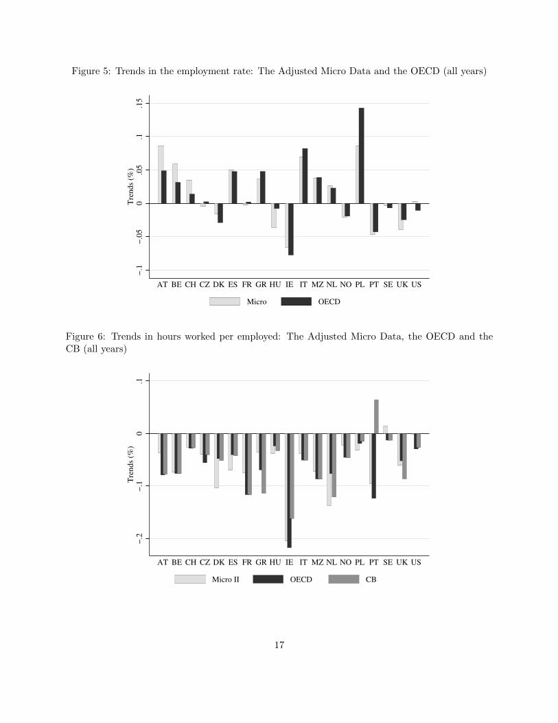
4.3.3 Trends

We calculate trends by computing the percentage difference between the mean of the last three sur-

vey years and the first three survey years for the employment rate and hours worked per employed.

Here, we do not show deviations from the Adjusted Micro Data, but include the Adjusted Micro

Data trend, so that one can easily see whether trends go in the same direction. The results are

shown in Figures 5 and 6. We want to stress that these numbers are not intended for cross-country

comparisons, since the time trends refer to different periods across countries.19

For the employment rates (Figure 5), the earliest data available for the OECD employment rates

stems from 1999.20 The trends over this short period of time line up quite well. For 3 countries,

trends go in a different direction for the Adjusted Micro Data and for the OECD, namely Czech

Republic, France and the US, but they are also very close to zero. Overall, trends match very

closely, with the largest deviations arising in Poland with around 6 percentage points.

19The exact numbers corresponding to the figures can be found in Web Appendix W.6 in Tables W.5 and W.6.20The only exception being the US, where we have data from 1983 onwards, and Greece, where data starts in

1998. Later starting points are 2000 for Ireland, Norway and the UK, 2001 for Sweden, 2003 for France and 2005 forGermany and Switzerland.

16

Figure 5: Trends in the employment rate: The Adjusted Micro Data and the OECD (all years)

−.1

−.0

50

.05

.1.1

5T

rends

(%)

AT BE CH CZ DK ES FR GR HU IE IT MZ NL NO PL PT SE UK US

Micro OECD

Figure 6: Trends in hours worked per employed: The Adjusted Micro Data, the OECD and theCB (all years)

−.2

−.1

0.1

Tre

nds

(%)

AT BE CH CZ DK ES FR GR HU IE IT MZ NL NO PL PT SE UK US

Micro II OECD CB

17

The generally good overlap of trends is also confirmed for hours worked per employed (Figure

6). Here, the most significant deviation arises for Portugal, where the CB indicates a positive trend,

while the Adjusted Micro Data and the OECD indicate a significant negative trend.21

Overall, trends match up fairly well between the Adjusted Micro Data and the OECD or the

CB. While we see differences in levels, it is not clear whether the macro data sets are more reliable

than our data, as the discussion of the US case shows.

5 Hours Worked of Men and Women: Recent Cross-Section

In this section, we describe hours worked for men and women aged 15 to 64 in the recent cross-

section. All results refer to averages of the years 2003-2007, i.e. before the crisis hit. The effect of the

crisis on hours worked will be analyzed separately in Section 7. We take averages over some years

in order to avoid that non-synchronized business cycles influence the results too heavily. We show

results grouping European countries by their geographical location into Scandinavia (Denmark,

Norway, and Sweden), Eastern Europe (Czech Republic, Hungary, and Poland), Western Europe

(Austria, Belgium, France, Germany, Ireland, Netherlands, Switzerland, and the United Kingdom),

and Southern Europe (Greece, Italy, Portugal, and Spain). Subsection 5.2 presents results as

unweighted averages for the respective country groups.

5.1 Differences in Hours Worked between Men and Women

Figure 7 presents average hours worked per person aged 15 to 64.22 The black bar refers to female

hours worked, the cumulated black and grey bars to male hours worked, and the line within the grey

bar to overall hours worked per person. Starting with average hours worked across both genders,

there is a large, well-known difference in hours worked per person between the US and Europe,

amounting on average to more than 200 hours, but surprising homogeneity across the different

European country groups.23 This homogeneity however hides substantial variation of male and

female hours worked per person within Europe.

While for the US both male and female hours worked are high with 1570 hours for men and

1140 hours for women, female hours worked per person are lower but still relatively high with 960

and 900 hours on average in Scandinavia and Eastern Europe, and lowest in Western Europe and

Southern Europe with 830 and 820 hours. By contrast, Western and Southern European countries

exhibit on average higher male hours worked than Scandinavian and Eastern European countries.

As a result, the gender hours gap is somewhat similar in the US, Scandinavia, and Eastern Europe,

21Only for Sweden do trends otherwise point in different directions, but again they are very close to zero.22The values corresponding to Figures 7-9 can be found in Tables A.7-A.9 in Appendix A.5.23The country outliers within Europe are Switzerland, with hours worked per person very close to the US level,

and Italy, with hours worked per person below 1000.

18

Figure 7: Average Hours Worked per Person (2003-2007): Full sample, Men and Women

0250

500

750

1,0

00

1,2

50

1,5

00

Scandinavia

Eastern EuropeWestern Europe

Southern Europe

US DK NO SE CZ HU PL AT BE CH DE FR IE NL UK ES GR IT PT

Female Male

but much larger in Western and Southern Europe.24 Overall, women and men exhibit similar

cross-country variation: while the standard deviation and thus the absolute variability of female

hours worked per person is with 116 hours slightly lower than the standard deviation of male hours

worked per person with 129 hours, in relative terms women exhibit larger cross-country variation

than men. The coefficient of variation of female hours worked per person amounts to .13, while for

male hours worked per person it is .09.

Figures 8 and 9 show the analogous numbers for the employment rate and hours worked per

employed separately. While Figure 7 already showed that surprising homogeneity in hours worked

per person within Europe masks substantial differences by gender, these two figures further show

substantial heterogeneity across country groups, but quite some homogeneity within country groups,

in how hours worked per person are split into the employment rate and hours worked per employed.

The male employment rate is uniformly high between roughly 70 and 80 percent, with the

notable exceptions of Hungary and Poland, where low employment rates are driven by older indi-

viduals who were educated and experienced most of their on-the-job training under Socialism.25

Female employment rates, however, show substantial variation, being highest in Scandinavia with

more than 70 percent, followed by the US and Western Europe, and being substantially lower in

24Within the country groups, the Czech Republic and Switzerland stand out with high female and male hours workedby Eastern respectively Western European standards, while Italy has very low hours for both genders compared tothe rest of Southern Europe.

25Results by age group are available from the authors upon request.

19

Figure 8: Average Employment Rate (2003-2007): Full sample, Men and Women

010

20

30

40

50

60

70

80

Scandinavia


Southern Europe


Figure 9: Average Hours Worked per Employed (2003-2007): Full sample, Men and Women

0400

800

1,2

00

1,6

00

2,0

00

Scandinavia


Southern Europe


Female Male

Eastern and Southern Europe with only around 50 percent. The country group ordering for women

is opposite when it comes to hours worked per employed: these are highest in the US and Eastern

20

Europe, closely followed by Southern Europe, and substantially lower in Scandinavia and Western

Europe. For men, the country group ordering of hours worked per employed is similar, but the

differences are much smaller than for women. The standard deviations and coefficients of varia-

tion across countries are much larger for female employment rates and hours worked per employed

than for the corresponding male numbers. For employment rates, the standard deviations are 9

and 6 respectively for women and men, while for hours worked per employed they are 196 and

120 respectively. As a result, the coefficients of variation are more than twice as large for women

as for men, amounting to .15 vs. .08 for employment rates, and .13 vs. .06 for hours worked per

employed. Thus, women are an especially interesting group to analyze if one wants to understand

cross-country differences in hours worked.

Figure 10: Female Hours Worked per Employed and the Employment Rate (2003-2007)

ATBE

CH

CZ

DE

DK

ES

FR

GRHU

IEIT

NL

NO

PL

PT

SEUK

US

Corr = −.58

1000

1200

1400

1600

1800

2000

Fem

ale

HW

E

40 50 60 70 80 Female ER

Figure 10 shows the negative correlation between female employment rates and female hours

worked per employed across countries, with a correlation coefficient of −.58. The US and the

Netherlands are somewhat outliers here: both have similar female employment rates of around 65

percent, but US employed women work on average more than 1700 hours opposed to the “predicted”

1400 hours, while Dutch employed women work only slightly more than 1100 hours. Adding up

female and male hours and employment rates, the aggregate correlation between employment rates

and hours worked per employed is −.57. This is however driven by the large negative correlation

for women; for men alone, the correlation coefficient is less than half the size, namely −.24.

Thus, a first stylized fact that we find in our data is a that in countries with high female

21

employment rates, the average employed woman works relatively few hours. This could be driven

by supply side effects, with the marginal woman entering employment exhibiting lower productivity

and choosing lower hours, or demand side effects, with countries that offer higher flexibility in

choosing individual hours being more successful in attracting more women into the labor force.

The next subsection will provide more evidence on this correlation.

5.2 Marriage and Children

When analyzing differences of male and female hours worked, two natural factors that could lead

to divergent labor market behavior by gender are marriage and children. Marriage allows for intra-

household specialization in home production vs. market work, and in some countries leads to tax

treatment that favors specialization, while children affect the labor supply of women typically more

than the one of men. In this Subsection, we therefore analyze how hours worked differ by marital

status and presence of children. We differentiate between preschool children, aged 0 to 4, and school

children, aged 5 to 14. Three words of caveat are necessary. First, marriage and children are of

course endogenous variables, also correlated with other variables like age. Thus, we can only show

correlations here and clearly not state any causal effects. We will point to possible other covariates

driving the results whenever approrpriate. Secondly, we distinguish individuals by marital status,

not cohabitation. This is largely driven by data needs, as cohabitation cannot clearly be identified

for most countries and years. Nevertheless, we are able to show later in this subsection that in

this recent cross-section differences between splitting the sample by marriage or cohabitation are

minor. Third, Scandinavia has to be taken out in this analysis, as the data from Scandinavia does

not allow us to identify whether children are present in the household.

Figure 11 shows the cross-sectional decomposition of male hours worked per person. The fol-

lowing three figures are set-up analogously. Panel (a) of the figure shows male hours worked per

person in the US by marital status and presence of children. Contrary to the following three figures,

which refer to female hours, we do not distinguish the group of the unmarried men by presence of

children. Unmarried men with children in the household are a very small group, and are a very

special group, combining widowers and divorced parents where the children live with the father,

with a group of cohabiting men, which much more resemble married men with children.26

Panel (b) of the figure decomposes the differences of the three European country groups to the

US into the demographic subgroups. We follow the decomposition approach put forth in Blundell

et al. (2013). Overall hours worked in country j are the average of hours worked by different

subgroups i, in our case married and unmarried individuals without, with preschool, or with school

26The hours worked of unmarried men with children also show large changes in the US time series, likely reflectingthe rise of cohabitation.

22

children, weighted by their population weights qi,j :

Hj =I∑

i=1

qi,jHi,j ,

Following Blundell et al. (2013), we can then decompose the difference in hours worked between

country j and the US into a structural effect Sj and a behavioural effect ∆j . The structural effect

is caused by differences in the population structure

Sj =

I∑i=1

Hi,j(qi,j − qi,US),

while the behavioural effect is the sum of the differences in hours worked, weighted by the US

population weights:

∆j =I∑

i=1

qi,US(Hi,j −Hi,US).

Structural and behavioral effects are depicted in Panel (b). Specifically, we show here directly

the sum of the structural effects Sj , but show the behavioral effects qi,US(Hi,j − Hi,US) for each

demographic group i separately. The panel should be read as follows: While in the US male hours

worked per person amount to 1569, in Eastern Europe they only amount to 1287. The first light

part of the bar shows that around 100 hours of this difference can be attributed to unmarried

men without kids, and so on for the following color parts. The 100 hours difference attributed to

unmarried men without kids reflects the combination of differences in behavior of this group in

the US and Eastern Europe, and their relative size in the overall US male population. The last,

black part of the bar represents differences that arise between the US and Eastern Europe due to

differences in the population structure. Thus, while e.g. the group of unmarried individuals likely

comprises more young and more old individuals than the group of married individuals, this is in

principle true for all countries. If differences in marriage or fertility rates, or marriage or fertility

by age, across countries played a large role in explaining cross-country differences, this would show

up as a large black part of the bar. Panel (c) repeats in the black bars the information shown in

panel (b), and adds in the light bar the “pure behavioral” effect that shows the difference in hours

between the US and the different European country groups for the respective demographic group,

without weighing the latter by the group size in the US, i.e. Hi,j −Hi,US . The first group of bars

refers to Eastern Europe, the next to Western Europe, and the last to Southern Europe. Within

each country group, we show results for all married, those with preschool and those with school

children, and then for unmarried (where for women we also add those with preschool and those

with school children), always maintaining this ordering.27

27We opt for showing all married and unmarried individuals together rather than those without children to be able

23

As panel (a) of Figure 11 shows, in the US married men work more than unmarried men,

and married men with children work more than those without children. Note that the latter

group comprises men whose children are older than 16 years. The difference between married

and unmarried men, which is absent for women, as we will show later, is driven by unusually low

employment rates among unmarried men in the US (results for the intensive and the extensive

margin for men are available upon request). Panel (b) repeats the differences in hours worked

per person between the US and the European country groups already reported in the previous

subsection: US men work around 300 hours more than Eastern European ones, and around 200

hours more than Western and Southern European ones. A negligible part of that can be attributed

to differences in the demographic structure between the US and Eastern and Southern Europe, while

around 10 percent of the difference to Western Europe comes from different demographic structures.

Focusing on individual demographic groups in panel (c) reveals fairly constant differences between

the US and Europe for married men, regardless of the presence of children or not. For unmarried

men (the last bar in each country group), the differences are smaller than for married men in

Western and Southern Europe. Since in the US married men work more than unmarried men, this

implies that hours worked of married and unmarried men in these two country groups are more

similar than in the US. Only for Eastern Europeans do we find similar differences to the US among

married and unmarried men. The low hours by unmarried men in Eastern Europe are driven

by the extensive margin and capture again an age effect, driven by older individuals who spent

considerable time working in the Socialist labor market. In weighted terms in panel (b) married

men without kids play the largest role in explaining differences between Europe and the US, while

for Eastern Europe unmarried men without kids are also important in explaining this difference.

Figure 12 shows the same information on hours worked per person for women, this time also

distinguishing by the presence of children for unmarried individuals. In the US, married and

unmarried women work very similar hours. Women with preschool children always work less hours

than women with school children, but at a higher level for unmarried than for married women.

Compared to over 1100 hours in the US, women work 200 hours less in Eastern Europe, and more

than 300 hours less in Western and Southern Europe. Thus, while for Eastern Europe the difference

to the US is larger for men than for women, it is the other way round for Western and Southern

Europe. As panel (b) shows, the demographic structure is only important in explaining differences

to the US for Eastern Europe, where it actually would indicate higher hours than in the US. Looking

at the different subgroups, it becomes clear that unmarried women with children, and especially

with school children, show the largest behavioral difference: the latter groups works fairly uniformly

700 hours less in Europe than in the US (see panel (c)). While the groups of unmarried women

with children are relatively small, panel (b) shows that the large behavioral differences lead to the

fact that they still account for a substantial part of the overall difference to the US, namely around

ot quickly gauge differences by marital status only.

24

14 to 24 percent. Among all unmarried women, not decomposing by the presence of children, and

married women with or without kids, the differences to the US are again fairly uniform, with a

few notable exceptions being married women with preschool kids in Southern Europe, which work

almost as much as in the US, and married women with school children in Eastern Europe, which

work even more than in the US.

25

Figure 11: Cross-sectional decomposition of male hours worked per person

(a) Male hours worked per person in the US (2003-2007) bymarital status and children

0500

1,0

00

1,5

00

2,0

00

Married Unmarried

All All PS kids SCH kids All

(b) Decomposition of difference to US in male hours workedper person (2003-2007)

1569

1346

1569

1287

1569

1373

1200

1300

1400

1500

1600


Southern Europe

US US US

Unmarried Men without Kids (.44) Unmarried Men with SCH Kids (.01) Unmarried Men with PS Kids (.01)

Married Men without Kids (.3) Married Men with SCH Kids (.11) Married Men with PS Kids (.13)

Difference in Structure

(c) Weighted and unweighted difference to US (2003-2007)by marital status and children

−300

−200

−100

0

EE WE SE

M, AllM, PS

M, SCHUM, All

M, AllM, PS

M, SCHUM, All

M, AllM, PS

M, SCHUM, All

Weighted Unweighted

26

Figure 12: Cross-sectional decomposition of female hours worked per person

(a) Female hours worked per person in the US (2003-2007)by marital status and children

0500

1,0

00

1,5

00

Married Unmarried

All All PS kids SCH kids All PS kids SCH kids

(b) Decomposition of difference to US in female hours workedper person (2003-2007)

1144

814

1144

900

1144

811

800

900

1000

1100

1200


Southern Europe

US US US

Unmarried Women without Kids (.38) Unmarried Women with SCH Kids (.04) Unmarried Women with PS Kids (.04)

Married Women without Kids (.31) Married Women with SCH Kids (.1) Married Women with PS Kids (.12)



−800

−600

−400

−200

0

EE WE SE

M, AllM, PS

M, SCHUM, All

UM, PSUM, SCH

M, AllM, PS

M, SCHUM, All

UM, PSUM, SCH

M, AllM, PS

M, SCHUM, All

UM, PSUM, SCH

Weighted Unweighted

27

Figure 13: Cross-sectional decomposition of the female employment rate

(a) Female employment rate in the US (2003-2007) by mar-ital status and children

020

40

60

80

Married Unmarried


(b) Decomposition of difference to US in female employmentrate (2003-2007)

65.5

60.6

65.5

51.4

65.5

50.5

45

50

55

60

65

70

75


Southern Europe

US US US





−40

−30

−20

−10

0

EE WE SE

M, AllM, PS

M, SCHUM, All

UM, PSUM, SCH

M, AllM, PS

M, SCHUM, All

UM, PSUM, SCH

M, AllM, PS

M, SCHUM, All

UM, PSUM, SCH

Weighted Unweighted

28

Figure 14: Cross-sectional decomposition of hours female worked per employed

(a) Female hours worked per employed in the US (2003-2007)by marital status and children

0500

1,0

00

1,5

00

2,0

00

Married Unmarried


(b) Decomposition of difference to US in female hours workedper employed (2003-2007)

1746

1346

1746 1746 1746

1603

1300

1400

1500

1600

1700


Southern Europe

US US US





−600

−400

−200

0200

EE WE SE

M, AllM, PS

M, SCHUM, All

UM, PSUM, SCH

M, AllM, PS

M, SCHUM, All

UM, PSUM, SCH

M, AllM, PS

M, SCHUM, All

UM, PSUM, SCH

Weighted Unweighted

29

The large differences in hours worked per person between the US and Europe among unmarried

women with children, together with the relative homogeneity of hours worked of this group within

Europe, points to the fact that the main driver of these country differences lies in the US. A likely

candidate are the Clinton welfare reforms, which gave single mothers strong incentives to enter the

labor force. There might thus be scope to increase hours worked for this group in Europe through

similar welfare reforms. Despite the relatively small size of this group, this would still close the gap

to the US by a significant number. A second interesting fact is that the difference of women with

preschool children in Europe to those in the US is largest for Eastern Europeans, and smallest for

Southern Europeans, with the same ordering, though at a different level, among unmarried and

married women. This seems to indicate that child care opportunities or cultural effects that affect

both unmarried and married women to the same extent might play a role in explaining labor supply

of women with preschool children.

The US picture for both female employment rates (panel (a) in Figure 13) and female hours

worked per employed (panel (a) in Figure 14) resembles very much the one for female hours worked

per person. Focusing on female employment rates, the differences to the US are again largest for

unmarried women with children, especially with school children, for every single European country

group (panel (c) in Figure 13). The differences are overall larger for unmarried than for married

women, which is true for every single subgroup (with or without children) and for each European

region. The heterogeneity of differences to the US across demographic subgroups is largest in

Eastern Europe and still substantial in Southern Europe, but smaller in Western Europe.

By contrast, the differences in hours worked per employed to the US (shown in Figure 14)

are relatively homogeneous for the different demographic subgroups within Eastern and Southern

EUorpe, but somewhat larger in Western Europe. Thus, employment rate differences explain

most of the demographic heterogeneity in Eastern and Southern Europe, but hours worked per

employed differences are mostly responsible for the demographic heterogeneity in Western Europe.

Hours worked per employed differences to the US are relatively small for all Eastern European

demographic groups, where overall female hours worked per employed are exactly equal to the ones

in the US, and very large for each of the Western European demographic subgroups, where overall

the difference amounts to 400 hours.

The negative cross-country correlation between female employment rates and female hours

worked per employed is actually present for each single demographic subgroup, with the exception

of married women with school children, where it is negative, but essentially zero (see Table 3). It

is especially large for the unmarried, where it amounts to -.6, -.5, and -.3, respectively, for women

without kids, women with preschool kids, and women with school kids.

Overall, we find that when looking at male hours worked per person, differences of European

country groups to the US are larger for married than for unmarried men, but do not depend

much on the presence of children, and are also quite homogeneous across Europe. For women,

30

Table 3: Cross-country correlation between female ER and female HWE

Correlation HWE-ER

Married

No kids −0.19

Preschool kids −0.26

School kids −0.03

Unmarried

No kids −0.60

Preschool kids −0.50

School kids −0.30

unmarried women with children stand out as the group showing the largest difference, which is

likely driven by the Clinton welfare reforms in the US. The decomposition of any female hours

worked per person difference into an extensive and an intensive margin shows as a robust fact across

all demographic subgroups that the extensive margin matters most in Southern Europe, while the

intensive margin matters most in Western Europe. Extensive margin differences show a lot of

heterogeneity across demographic groups in Southern and Eastern Europe, while intensive margin

differences exhibit high heterogeneity in Western Europe. Thus, to explain international differences

in hours worked research should focus on factors which could explain the relative homogeneity in

male hours differences to the US across different demographic subgroups, together with the large

heterogeneity in female hours worked differences, as well as their decompositions into extensive and

intensive margins. The large differences in the labor supply behavior of unmarried women with

children point to welfare systems playing a role, but child care, taxation of married couples, divorce

risks, gender wage gaps, and cultural factors likely also play a role. We will specifically address the

flexibility of the labor market as potential factor in Section 5.4.

Figures A.1 to A.4 in Appendix A.6 replicate all results from this subsection, but splitting

the sample by cohabitation, not marriage. Since we do not have cohabitation information for

all countries and years, we repeat the results splitting by marriage on the left hand side using

the sample for which we also have cohabitation information, while the new results splitting by

cohabitation are shown on the right hand side. Overall, results are very similar and mostly almost

non-distinguishable whether the sample is split by marriage or cohabitation. The only significant

difference that arises comes for men in Western Europe: while unmarried men in Western Europe

work around 90 hours less than their US counterparts, non-cohabiting men work around 140 hours

less. This difference is driven by the behavior of Western Europeans, not US citizens, where hours

worked of unmarried or non-cohabiting men are virtually the same. It indicates that cohabiting

but unmarried men in Western Europe resemble in their work behavior more married men (who

31

work more than unmarried ones) than cohabiting but unmarried men in the US. Note also that

average cohabitation rates in Western Europe are with 10 percent twice as large as cohabitation

rates in the other regions.

5.3 Hours Worked Dispersion

Our data also allow us to analyze the dispersion of hours worked within a county. Since we find that

high employment rates are associated with low hours worked per employed, it would be interesting

to see how spread out the distribution of hours worked is in different regions. Part-time work is

best captured by looking at usual weekly hours worked, and for expositional purposes we call any

job involving less than 30 usual weekly hours a part-time job. Figure 15 shows the cumulative

distributions of usual weekly hours worked for men in panel (a) and for women in panel (b),

conditional on working. For men, full-time work is the prevalent form of employment in all country

groups, with “full-time” amounting to slightly less than 40 hours in Scandinavia and some Western

European countries. Male part-time work is most prevalent in Scandinavia, but even there amounts

to only 10% of men working 30 hours or less, and almost completely absent in Eastern and Southern

Europe. For women, part-time work is quite prevalent in Western Europe and Scandinavia, but

almost absent in Eastern Europe. 40% of Western European and 30% of Scandinavian women work

30 hours or less per week, while less than 10% of Eastern Europeans do that. The distributions of

usual hours worked are surprisingly quite similar in the US and Southern Europe, where in both

around 20% of women work 30 hours or less. Overall, for men there is more heterogeneity across

country groups in the upper tail of the usual hours distribution, while for women it is clearly at the

lower tail. Thus, the prevalence of part-time work still shows significant variation across regions.

32

Figure 15: Cumulative distribution of usual weekly hours worked

(a) Men (2003-2007)

02

04

06

08

01

00

Pe

rce

nta

ge

s o

f th

e p

op

ula

tio

n

10 20 30 40 50 60 Usual weekly hours worked

US Scandinavia Western Europe

Eastern Europe Southern Europe

(b) Women (2003-2007)

020

40

60

80

100

Per

centa

ges

of

the

popula

tion




33

5.4 Supply vs. Demand of Part-Time Jobs

The previous subsection documented a high prevalence of female part-time work in Western Europe

and Scandinavia, but a low prevalence in the US, Southern Europe, and especially Eastern Europe,

similar to the different decomposition of female hours worked per person in an extensive and

an intensive margin in Western Europe/Scandinavia vs. Eastern/Southern Europe. Moreover,

Subsection 5.2 documented a high heterogeneity across demographic subgroups in employment

rates for Southern and Eastern Europe, and in hours worked per employed for Western Europe. A

big question that arises in the analysis so far is whether women in Southern and Eastern Europe

do not want to work part-time more frequently, as their counterparts in Western Europe and

Scandinavia do, or whether there is a scarcity of part-time jobs in Southern and Eastern Europe

that forces women to work full-time. In the first case, a negative correlation between employment

rates and hours worked per employed could arise due to self-selection into employment according

to ability: in countries, which give lots of incentives to work, the employment rate will be high, but

the marginal woman will be of a comparatively low ability type and thus optimally decide to work

few hours. In the second case, part-time jobs are simply not offered by firms, leading naturally

to high hours worked per employed, but at the same time to low employment rates, as low ability

women or women who desire less labor market involvement for other reasons, e.g. the presence of

small children, will rather opt out of the labor market.

The variability of employment rates and hours worked per employed across different subgroups

within a country could give some indication about whether the availability of part-time jobs or the

demand for part-time jobs drive the decomposition into employment rates and hours worked per

employed. If in country A only full-time jobs are available, we should naturally see a low variability

of hours worked per employed across demographic subgroups, but a high variability of employment

rates, as individuals in subgroups that desire less labor market involvement (e.g. low educated

women, or women with preschool children) will be less likely to work at all if they are forced to

work full-time. On the other hand, if in country B individuals have full flexibility in choosing their

hours worked, then individuals who desire less labor market involvement will adjust along both

the extensive and the intensive margin (e.g. women with preschool children might be less likely

to participate in the labor market, and also choose lower hours conditional on participation). As

a result, the within-country variability of employment rates across demographic subgroups would

be lower in country B than in country A, but the variability of hours worked per employed would

be higher. Thus, if the availability of part-time jobs in Western Europe and its absence in Eastern

and Southern Europe drives the different decompositions into extensive and intensive margins, we

should expect a higher variability in hours worked per employed across demographic subgroups in

Western Europe than in Southern and Eastern Europe, but a lower variability in employment rates.

Table 4 analyzes this formally by showing regional coefficients of variation for employment

rates and hours worked per employed across the six demographic subgroups from Section 5.2. The

34

Tab

le4:

Coeffi

cien

tof

Var

iati

onin

Em

plo

ym

ent

Rat

ean

dH

ours

Wor

ked

per

Em

plo

yed

by

Mar

ital

Sta

tus

an

dP

rese

nce

of

Ch

ild

ren

Country

ER

HW

E

Eas

tern

Eu

rop

e0.3

60.

07

Wes

tern

Eu

rop

e0.1

30.

14

Sou

ther

nE

uro

pe

0.1

60.

05

Un

ited

Sta

tes

0.0

90.

04

Tab

le5:

Em

plo

ym

ent

Rat

ean

dH

ours

Wor

ked

per

Em

plo

yed

by

Ed

uca

tion

Population

Share

sEmploymentRate

Hours

Work

ed

perEmployed

Country

Low

Med

ium

Hig

hL

owM

ediu

mH

igh

CV

Low

Med

ium

Hig

hC

V

Sca

nd

inav

ia0.2

0.45

0.30

0.52

0.75

0.85

0.3

511

37.5

1333.

31438.

70.

18

Eas

tern

Eu

rop

e0.2

40.

620.

140.

230.

570.

780.7

016

90.7

1771.

91729.

80.

06

Wes

tern

Eu

rop

e0.3

10.

450.

220.

440.

670.

810.4

212

31.4

1331.

41478.

90.

14

Sou

ther

nE

uro

pe

0.5

30.

300.

170.

390.

550.

770.4

716

07.2

1633.

51557.

20.

05

Un

ited

Sta

tes

0.1

40.

500.

350.

370.

650.

770.4

814

62.9

1721.

41831.

00.

17

35

coefficient of variation is constructed by first building country-specific coefficients of variation across

the six demographic subgroups, and then taking the average of these coefficients of variations over

all countries in a given region.28 As the table shows, Western European countries have a lower

within-country variability of employment rates than Southern and especially Eastern European

countries, but a more than twice as large within-country variability of hours worked per employed

compared to Southern and Eastern European countries. It is noteworthy that the US as a country

with both high employment rates and high hours worked per employed is also an outlier here,

by exhibiting low coefficients of variation in the within country variability of both employment

rates and hours worked per employed across the demographic subgroups. Goldin (2014) stresses

in the Presidential Address to the American Economic Association that temporal flexibility is the

main way to close the last chapter of the grand gender convergence in the US. While her notion of

temporal flexibility is broader than simple part-time work, our results reinforce her thesis to some

extent.

Table 5 analyzes education group rather than demographic subgroups, and shows population

shares, employment rates, and hours worked per employed of the three education groups low,

medium, and high education, always presenting averages across all countries in a region. Addition-

ally, columns 7 and 11 present the coefficients of variation along the extensive and the intensive

margin. As the table shows, the education-gradient in employment rates is steeper in Eastern

and Southern Europe than in Western Europe and Scandinavia, while the opposite is true for the

education-gradient in hours worked per employed, where in fact Eastern and Southern Europe

show a U-shape across education groups. Consequently, the coefficients of variation across edu-

cation groups are larger in Southern and especially Eastern Europe than in Western Europe and

Scandinavia for employment rates, but less than half of the size when it comes to hours worked per

employed.

Overall, this evidence indicates that there might be a scarcity of offered part-time jobs relative

to their demand in Southern and Eastern Europe, forcing all women there to work a large number of

hours if they choose to work, and thus resulting in larger within-country variability in employment

rates than in Western Europe and Scandinavia, where it seems easier to find a part-time job.

Of course, there is still room for self-selection by ability leading to a negative correlation of

employment rates and hours worked per employed. However, this self-selection would have to

take place within education group, while being absent across groups, which is less likely. Also,

the population shares by education differ somewhat across regions, as Table 5 shows, potentially

driving part of the results. Still, it is difficult to reconcile this evidence with a story that explains

the negative correlation between mean employment rates and hours worked per employed across

countries exclusively by self-selection.

28When building country-specific coefficients of variation, we divide the unweighted standard deviation acrosseducation groups by the unweighted mean over the six demographic subgroups.

36

5.5 Cross-Section: Summary

Summarizing, we find that a relative homogeneity of hours worked per person within Europe hides

significant heterogeneity across gender and across the extensive and intensive margin. Female

hours worked are especially low in Southern and Western Europe, where male hours worked are

even slightly above the European average. The US stands out with high hours worked for both

genders. High female employment rates coupled with low hours worked per employed in Western

Europe and Scandinavia, with the opposite being true in Southern and Eastern Europe, lead to

a strong negative cross-country correlation between female employment rates and hours worked

per employed. Looking at different demographic subgroups, this negative correlation is present

regardless of marital status and presence or absence of children. Low female hours worked per

employed in Scandinavia and Western Europe are driven by a large prevalence of part-time work.

We present some evidence that a lack of offered part-time job rather than a missing desire to work

part-time ar at the root of low part-time rates in Eastern and Southern Europe.

6 Hours Worked of Men and Women: Time Trends

In this section, we analyze time trends in the development of hours worked for men and women.

We compare three time periods: 1983-1987, 1993-1997, and 2003-2007. The first time period does

not cover the full set of countries, but from the second time period on all countries are included.29

We analyze hours worked per person, the extensive and the intensive margin, and the distribution

of hours.

6.1 Developments from the 1980s to the 2000s

29However, for some countries from the ELFS we do not have information for all five years 1993 to 1997, but onlythe last ones: Austria, Norway, and Sweden start in 1995, Hungary and Switzerland in 1996, and the Czech Republicand Poland in 1997.

37

Fig

ure

16:

Tre

nd

sin

Mal

eH

ours

Wor

ked

and

Em

plo

ym

ent

Rat

es

(a)

HW

P,

80’s

to90’s

BE

DE

FR

IE

NL

UK

ES

GR

IT

PT

US

DK

100012001400160018001993−1997

10

00

12

00

14

00

16

00

18

00

19

83

−1

98

7

(b)

ER

,80’s

to90’s

BE

DE

FR

IE

NL

UK

ES

GR

IT

PT

US D

K

607080901993−1997

60

70

80

90

19

83

−1

98

7

(c)

HW

E,

80’s

to90’s

BE

DE

FR

IE

NL

UK

ES

GR

IT

PT

US

DK

16001800200022001993−1997

16

00

18

00

20

00

22

00

19

83

−1

98

7

(d)

HW

P,

90’s

to2000’s

AT

BE

CH

DE

FR

IE

NL

UK

CZ

HU

PL

ES

GR

IT

PT

US

DK

NO

SE

100012001400160018002003−2007

10

00

12

00

14

00

16

00

18

00

19

93

−1

99

7

(e)

ER

,90’s

to2000’s

AT

BE

CH

DE

FR

IE

NL

UK

CZ

HU

PL

ES

GR

IT

PT

US

DK

NO

SE

607080902003−2007

60

70

80

90

19

93

−1

99

7

(f)

HW

E,

90’s

to2000’s

AT

BE

CH

DE F

R

IE

NL

UK

CZ

HU

PL

ES

GR

IT

PT

US

DK

NO

SE

16001800200022002003−2007

16

00

18

00

20

00

22

00

19

93

−1

99

7

38

Fig

ure

17:

Tre

nd

sin

Fem

ale

Hou

rsW

orke

dan

dE

mp

loym

ent

Rat

es

(a)

HW

P,

80’s

to90’s

BE

DEF

R

IEN

L

UK

ES

GR

IT

PT

US

DK

400600800100012001993−1997

40

06

00

80

01

00

01

20

01

98

3−

19

87

(b)

ER

,80’s

to90’s

BE

DE F

R

IE

NL

UK

ES

GR

IT

PT

US

DK

203040506070801993−1997

20

30

40

50

60

70

80

19

83

−1

98

7

(c)

HW

E,

80’s

to90’s

BE

DE

FR

IE

NLU

K

ES

GR

IT

PT

US

DK

1000120014001600180020001993−1997

10

00

12

00

14

00

16

00

18

00

20

00

19

83

−1

98

7

(d)

HW

P,

90’s

to2000’s

AT

BE

CH

DE

FR

IE

NL

UK

CZ

HU

PL

ES

GR

IT

PT

US

DK

NO

SE

7009001100130015002003−2007

70

09

00

11

00

13

00

15

00

19

93

−1

99

7

(e)

ER

,90’s

to2000’s

AT

BE

CH

DE

FR

IE

NL

UK

CZ

HU

PL

ES

GR

IT

PT

USD

KNO

SE

203040506070802003−2007

20

30

40

50

60

70

80

19

93

−1

99

7

(f)

HW

E,

90’s

to2000’s

AT

BE

CH

DE

FRIE

NL

UK

CZH

U

PL

ES

GR

IT

PT

US

DK

NO

SE

1000120014001600180020002003−2007

10

00

12

00

14

00

16

00

18

00

20

00

19

93

−1

99

7

39

Figure 16 presents time trends for male hours worked per person (left panel), the employment

rate (middle panel), and hours worked per employed (right panel) from the 1980s (1983-1987) to

the 1990s (1993-1997) (upper panel), and from the 1990s to the 2000s (2003-2007, lower panel).

In each graph, the x-axis shows the earlier time period, and the y-axis the later time period, such

that an alignment on the 45 degree line means no change, observations above the 45 degree line

represent an increase, and observations below the 45 degree line a decrease. Each dot represents a

country, with the country groups having different symbols (Scandinavia square, Southern Europe

triangle, Western Europe circle, Eastern Europe x, US diamond).

For men, hours worked per person decreased on average by 3.3 percent from the 1980s to the

1990s, driven by a decrease in the employment rate. In results not shown but available upon re-

quest, we show that this decrease is driven primarily by men aged 55 to 64: the employment rate

for men in this age group decreased substantially from the 1980s until around the mid 1990s, likely

due to an expansion of early retirement programs. Moreover, the employment rate of young men

aged 15 to 24 also decreased somewhat, while it remained essentially unchanged for the core age

group. From the 1990s to the 2000s, the picture for hours worked per person is more heterogeneous.

Employment rates tend to increase in the majority of countries, resulting in an average increase of

2 percentage points, while at the same time we observe a decrease in hours worked per employed of

on average 2.2 percent. The increase in the employment rate is driven by older individuals aged 55

to 64, caused by substantial pension reforms in many European countries which reversed the trend

of early retirement, while the slight decrease in hours worked per employed is more homogeneous

across age groups.30 For women, there is a clear trend increase of on average 11 percent in hours

worked per person from the 80s to the 90s and from the 90s to the 2000s, as Figure 17 shows.

While from the 80s to the 90s this trend is universal, in the later time period we see some cross-

country convergence, with largest increases in countries that started with the lowest female hours

worked per person in the 1990s. In both time periods, this increase in hours worked per person,

as well as the convergence in the later time period, are driven by increasing employment rates (on

average +6 percentage points in both periods). At the same time, hours worked per employed

were falling by on average -3.6 percent between the 80s and 90’s, and are rather stable between

the 90s and 2000s. The convergence in employment rates leads to the fact that employment rate

differences across countries are shrinking substantially: the maximum-minimum difference across

countries amounted to 43 percentage points in the 80s, 37 percentage points in the 90s, but only

27 percentage points in the 2000s.

30Age group results are available from the authors upon request.

40

Figure 18: Correlation between change in employment rate and change in hours worked per em-ployed

(a) 80’s to 90’s

BE

DK

ES

FR

GR

IE

IT

DE

NL

PT

UKUS

Corr = −.625

−15

−10

−5

05

10

15

20

% C

han

ge

in f

emal

e H

WE

80s

to 9

0s

−15 −10 −5 0 5 10 15 20Change in female ER 80s to 90s

(b) 90’s to 2000’s

BEDK

ES

FR

GR

IE

IT

DE

NL

PT

UK

US

AT

CH

CZ

HU

NO

PL

SE

Corr = −.29

Corr = −.178

−15

−10

−5

05

10

15

20

% C

han

ge

in f

emal

e H

WE

90s

to 2

000s

−15 −10 −5 0 5 10 15 20Change in female ER 90s to 2000s

Thus, as in the cross-section, we see in the time series that an increase in the employment rate

goes in hand with a fall in hours worked per employed (see Figure 18). In fact, the correlation

between the change in the employment rate and the change in hours worked per employed is -.63

for women in the time period 80s to 90s,31 falling in absolute size to -.18 in the later time period

(where it is still -.29 among the countries that were in the sample already in the 80s). This decrease

in the absolute size of the negative correlation seems to be driven by the increasing cross-country

convergence in employment rates, which is not accompanied by a convergence in hours worked per

employed.32

31The two countries that do not follow this pattern are the US and the UK, which achieved an increase in theemployment rate at the same time as an increase in hours worked per employed.

32The negative correlation between changes in employment rates and hours worked per employed is also presentfor men in the first time period, where it amounts to -.53, but disappears in the second time period.

41

6.2 Trends in Differences by Marital Status and Presence of Children

Figures 19 to 22 correspond to the cross-sectional figures on demographic subgroups, but compare

differences to the US in the 80s (1983-1987), the 90s (1993-1997) and the 2000s (2003-2007), where

the latter correspond to the numbers discussed already in Section 5.2. We omit panel (b) of the

Figures presented in Section 5.2, and instead split up the old panel (c) into married individuals (new

panel (b)) and unmarried individuals (new panel (c)). In each of panel (b) and (c), we present three

groups of bars corresponding to the three country groups. Within each group, we show the time

series development for all, and individuals with preschool and school children, respectively, with

the exception of unmarried men, whom we do not further decompose by the presence of children,

as before. The time series developments are represented by three bars, where the first bar refers

to the 80s (1983-1987), the second to the 90s (1993-1997), and the third to the 2000s (2003-2007).

Since the Eastern European countries entered the sample only in the 90s, the bar for the 80s is

omitted for this country group.

As panel (a) of Figure 19 shows, male hours worked per person were fairly stable over time in the

US for all demographic subgroups.33 Differences to the US increased from the 80s to the 2000s for

married men in all European country groups, mostly driven by married men without children. This

divergence happened between the 80s and the 90s for Western and Southern Europe, where from

the 90s to the 2000s differences mostly decreased, and from the 90s to the 2000s for Eastern Europe,

which we do not observe in the 80s. The increasing difference in male hours worked between the

US and Western and Southern Europe betweein the 80s and the 90s is likely driven by the increase

in early retirement programs in Europe. For unmarried men, by contrast, differences to the US

became smaller for Southern and Western Europe, but stayed stable for Eastern Europe. Thus,

given the stable hours in the US, this implies that married men decreased their hours in Europe

over the sample period, with the opposite being true for unmarried men.

33Note that despite the slight increase in hours worked per person of both married and unmarried men, overallhours worked per person slightly decreased from the 80s to the 2000s due to changes in the composition of bothgroups, with the group of unmarried men increasing in size.

42

Figure 19: Demographic decomposition of male hours worked per person over time

(a) Male hours worked per person in the US over time by thepresence of children

0500

1,0

00

1,5

00

2,0

00

Married Unmarried


80s 90s 2000s

(b) Weighted and unweighted difference to US for marriedmen over time, by the presence of children

−400

−300

−200

−100

0

All, EE PS, EE SCH, EE All, WE PS, WE SCH, WE All, SE PS, SE SCH, SE

Weighted Unweighted

(c) Weighted and unweighted difference to US for unmarriedmen over time

−400

−300

−200

−100

0

All, EE All, WE All, SE

Weighted Unweighted

43

Figure 20: Demographic decomposition of female hours worked per person over time

(a) Female hours worked per person in the US over time, bymarital status and children

0500

1,0

00

1,5

00

Married Unmarried


80s 90s 2000s

(b) Weighted and unweighted difference to US for marriedwomen over time, by the presence of children

−800

−600

−400

−200

0200


Weighted Unweighted

(c) Weighted and unweighted difference to US for unmarriedwomen over time, by the presence of children

−800

−600

−400

−200

0200


Weighted Unweighted

44

Female hours worked per person are increasing over time in the US (panel (a) of Figure 20).

For married women with children, the increase in hours worked is more pronounced in all European

country groups than in the US, thereby lowering the US-Europe gap. The opposite is true for mar-

ried women without children, leading to overall stable hours differences of married women between

the US and the European country groups, or even increasing ones in the case of Eastern Europe.

By contrast, for unmarried women without children the US-European difference is decreasing over

time, leading to decreasing or stable overall differences for unmarried women. The most remark-

able change comes from the large increase in the difference of hours worked for unmarried women

with preschool or school children between the US and all European country groups (panel (c)),

which is driven by the large increase in the hours of these two groups over time in the US (panel

(a)). Thus, we observe quite some differences in relative time trends for married and unmarried

women (stable/diverging vs. stable/converging) between Europe and the US, as well as between

women with and without children (in the case of married women, diverging without children and

converging with children, in the case of unmarried women the other way round).

Figures 21 and 22 show the decomposition of these trends in female hours worked per person

into an extensive and an intensive margin. In the US, hours increased for all subgroups along both

margins. Yet, the large increase for singles with children is mostly driven by the extensive margin,

bringing this group into the labor market. For unmarried women without children, as well as all

married women with and without children, we observe mostly a convergence in employment rate

differences between Europe and the US over time.34 For hours worked per employed, the difference

to the US becomes more negative for all demographic subgroups in all European regions. The

difference and the change are largest for Western Europe, but the uniformity of these trends in

hours worked per employed is striking. While hours worked per employed uniformly rise in the US,

they decrease in Europe.

If we analyze the cross-country correlation of changes in the employment rate and changes

in hours worked per employed for the different demographic subgroups, it is universly strongly

negative for the period 1980s to 1990s, except for married women with preschool children. In the

later time period (1990s to 2000s), it remains negative only for married women without children,

suggesting that it might be driven by older women.35

34An exception are married women without children in Eastern Europe.35Remember that women with children older than 16 years are categorized as women without children.

45

Figure 21: Demographic decomposition of female employment rates over time

(a) Female employment rate in the US over time, by maritalstatus and children

020

40

60

80

Married Unmarried


80s 90s 2000s


−30

−20

−10

010


Weighted Unweighted


−40

−30

−20

−10

010


Weighted Unweighted

46

Figure 22: Demographic decomposition of female hours worked per employed over time

(a) Female hours worked per employed in the US over time,controlling for marital status and children

0500

1,0

00

1,5

00

2,0

00

Married Unmarried


80s 90s 2000s


−600

−400

−200

0200


Weighted Unweighted


−600

−400

−200

0200


Weighted Unweighted

47

6.3 Dispersion Trends

Figures 23 and 24 show the cumulative distribution functions of usual weekly hours worked for men

and women for the three time periods 1983-1987, 1993-1997, and 2003-2007. For men in the 80s, the

distribution function almost collapses to a vertical line at 40 hours for the US and Scandinavia, with

usual hours exceeding 40 hours in Southern Europe, and Western Europe showing some variation

around 40 hours. By contrast, the 90s show a decrease in “typical” usual hours worked below 40

for Scandinavia, with Western Europe following suite in the 2000s, as well as more heterogeneity

in usual hours worked in general. This is in line with the decrease in hours worked per employed

for Western European and Scandinavian men in Figure 16.

For women, part-time work, which we define as working less than 30 hours, was most prominent

in the 80s in Scandinavia, and increased in importance in Western Europe from the 80s to the 90s,

overtaking the Scandinavian part-time work rate. It kept increasing in Western Europe into the

2000s, while the part-time work rate somewhat declined in Scandinavia in the latest period. At the

same time, part-time work lost importance in the US and gained importance in Southern Europe,

aligning the distributions for both regions. The part-time work rate in Eastern Europe is at a low

level in both the 90s and the 2000s. While the cross-country distribution of usual hours worked in

the 80s shows quite some heterogeneity at both the upper and the lower end of the distribution,

the distribution at the lower end clearly dominates in heterogeneity in the 2000s.

As an interesting fact emerges a positive correlation between changes in part-time work and

changes in the employment rate. Blau and Kahn (2013) relate the falling behind of the US female

participation rate in the international context in the 2000s to the increase of family-friendly policies

in other OECD countries. Indeed, as panel (b) of Figure 25 shows, there is a positive correlation

of 0.43 between the percentage point increase in the share of women working less than 30 hours

a week and the percentage point increase in the female employment rate between the 1990s and

the 2000s. Thus, the countries that experienced the strongest increase in the female employment

rate in this decade are the ones that also saw the largest increase in the share of women working

part-time. This correlation was even stronger in the time period 80s to 90s, where it amounted to

0.59.36 In unreported results, we find that the correlation between increases in the part-time share

and increases in the employment rate is especially large for unmarried women in the period 80s to

90s, but married women in the period 90s to 2000s. While the negative correlation between changes

in employment rates and hours worked per employed becomes weak in the later time period, there

is thus still a strong positive correlation between increases in the employment rate and part-time

work, supporting the claims by Blau and Kahn (2013) and Goldin (2014) that increases in flexibility

are the main step left to close the gender gap in the labor market. At the same time, the results

make clear that part-time work becomes a less important margin over time, and other areas of

flexibility, e.g. flexible work hours during the day, might become more important in the future to

36Keeping the sample of countries fixed, this would compare to a correlation of 0.53 in the 90s to 2000s.

48

retain women in the labor market, and allow them to make a career (which is beyond the scope of

this paper).

49

Figure 23: Trends in distribution of male usual hours worked

(a) 1983-1987

020

40

60

80

100

Per

centa

ges

of

the

popula

tion




(b) 1993-1997

020

40

60

80

100

Per

centa

ges

of

the

popula

tion




(c) 2003-2007

020

40

60

80

100

Per

centa

ges

of

the

popula

tion




50

Figure 24: Trends in distribution of female usual hours worked

(a) 1983-1987

020

40

60

80

100

Per

centa

ges

of

the

popula

tion




(b) 1993-1997

020

40

60

80

100

Per

centa

ges

of

the

popula

tion




(c) 2003-2007

020

40

60

80

100

Per

centa

ges

of

the

popula

tion




51

Figure 25: Increase in share of women working part-time vs. increase in female employment rate

(a) 80’s to 90’s

BE

DK

ES

FRGR

IE

IT

DE

NL

PT

UK

US

Corr = .54

−5

05

10

15

20

PP

Ch

ang

e in

Fem

ale

ER

−5 0 5 10 15 20PP Change in Share of Women < 30 hours/week

(b) 90’s to 2000’s

BE

DK

ES

FR

GR

IE

IT

DE

NL

PT

UK

US

ATCH

CZ

FI

HU

NO

PL

SE

Corr = .53

Corr = .425

−5

05

10

15

20

PP

Ch

ang

e in

Fem

ale

ER

−5 0 5 10 15 20PP Change in Share of Women < 30 hours/week

52

6.4 Time Trends: Summary

Summarizing, for men, employment rates first decrease from the 80s to the 90s and then increase

and converge across countries from the 1990s to the 2000s, in conjunction with a decrease in hours

worked per employed. This is driven by an increased participation in the labor market of men aged

55 to 64 from the mid 1990s on. Over the time frame 1980s to 2000s, the within-country dispersion

of usual hours worked increases somewhat for men, and the ”typical” weekly hours fall below 40 in

Western Europe and Scandinavia. For women, the employment rate increases throughout, though

at a decreasing rate, and shows some cross-country convergence. The decline in cross-country

differences relative to the US is present for every demographic subgroup but unmarried women

with children, due to the large increase in their employment rate in the US over time. By contrast,

hours worked per employed are consistently falling in Europe relative to the US over time. Recent

increases in female labor force participation in Europe go in hand with a fall in hours worked per

employed, and an increasing share of women working part-time. For both sexes, hours worked per

employed tend to decrease in Western Europe. Between the 1980s and the 1990s, we observe a

strong negative correlation between changes in the employment rate and changes in hours worked

per person for both men and women, while the negative correlation becomes much smaller for

women between the 1990s and the 2000s, and disappears for men.

7 The Great Recession

Last, we analyze the effect of the Great Recession on male and female hours worked.

7.1 Male and Female Hours Worked in the Great Recession

Figures 26 and 27 show the change in male and female, respectively, hours worked per person

during the great recession. To do that, they depict on the x-axis the average hours worked per

person in the pre-crisis period 2003-2007, and on the y-axis the corresponding hours in the crisis

period 2009-2011. For men, Figure 26 makes the strong universal effect of the crisis apparent.

Male hours worked per person decline substantially, except for Poland, Germany, and Sweden, and

with significant heterogeneity across countries. The largest decreases occur in Ireland and Spain

with 22 and 16 percent, respectively. But even disregarding these two countries, the mean decrease

amounts to 3.5 percent. Quite surprisingly, this decrease in hours due to the crisis is not present

for women. Figure 27 shows that for the majority of countries, female hours worked per person are

actually increasing during the crisis, with the notable exception of the US and Ireland, where they

are decreasing by 6.3 and 9.3 percent, respectively.

53

Figure 26: Change in male hours worked per person during the Crisis

AT

BE

CH

DE

FR

IE

NLUK

CZ

HU

PL

ES

GR

IT

PT

US

DKNO

SE

1100

1300

1500

1700

2009−

2011

1100 1300 1500 17002003−2007

Figure 27: Change in female hours worked per person during the Crisis

AT

BE

CH

DE FR

IE

NL

UK

CZ

HUPL

ES

GR

IT

PT

US

DKNO

SE

600

800

1000

1200

2009−

2011

600 800 1000 12002003−2007

54

7.2 Sectoral and Educational Effects

The smaller effect of the crisis on female hours worked is at first view surprising, given that the

literature typically finds that women exhibit a higher labor supply elasticity than men, suggesting

that they might adjust hours more over the cycle than men. On the other hand, the added worker

hypothesis would stipulate that in a model with intra-household insurance, the secondary earner

might enter the labor force or increase her hours when the primary earner loses his job in a recession

(see e.g. Lundberg (1985) and Stephens (2002)).

The question arises whether gender was indeed an underlying factor of differential effects during

the crisis, or whether the apparent gender difference in the previous two figures is in fact an

artefact of some omitted factors. One hypothesis might be that the crisis affected manufacturing

and construction jobs, which are predominantly male, more than service jobs. Different education

groups could also be affected differently, which might again affect men and women differentially.

Last, as we saw before, female hours worked exhibited an increasing trend in the pre-crisis period,

so that it could still be the case that this trend was dampened by the crisis without an actual

decline in female hours.

In order to investigate these hypotheses, we run the following regression. In the absence of

individual-level panel data, we first compute the employment rate and hours worked per employed

for each country and year for each gender/sector/education cell, focusing on 15 sectors and 3

education levels. The employment rate by gender/sector/education is defined as the number of

women working in this sector and exhibiting this education level, divided by the number of all

women, and analogously for men. Summing up across all sector/education cells thus gives the

aggregate gender-specific employment rates. We then regress the percent change in this employment

rate and the percent change in hours worked per employed for these gender/sector/education cells

between 2003-2007 and 2009-2011 (capturing the effect of the Great Recession) on a male dummy,

as well as the respective change between 1999-2002 and 2003-2007 (capturing any pre-crisis trends),

this pre-crisis trend interacted with the male dummy (allowing for different pre-crisis trends among

men and women, which we saw in Section 6.1), sectoral dummies, and education dummies.37 We

analyze percent changes rather than percentage point changes in the employment rate, such that

if the number of male and female workers in a given sector declines proportionally, as would be the

case for random dismissals, this leads to the same change in the employment rate. Thus, we run

the following regression, where the subscript g stands for gender, s for sector, e for education level,

37Thus, we first take average of the years 1999-2002, 2003-2007, and 2009-2011, and then look at the percentchanges between these averages.

55

and c for country:

∆crisisc,g,s,e = β0 + β1 ∗Male Dummyg + β2 ∗∆precrisis

c,g,s,e + β3 ∗∆precrisisc,g,s,e ∗Male Dummyg+∑

s

βs ∗ Sector Dummiess +∑e

βe ∗Education Dummiese +∑c

βc ∗Country Dummiesc + εc,g,s,e

Table 6: Regression of crisis change on precrisis change, male dummy, sector dummies, and educa-tion dummies

Employment Share Hours Worked per Employed

(1) (2) (1) (2)

Male Dummy −0.039*** 0.005 −0.012*** −0.009***(0.011) (0.009) (0.002) (0.002)

∆precrisis – 0.342*** – −0.026(0.026) (0.027)

∆precrisis∗ Male Dummy – −0.163*** – −0.032(0.037) (0.042)

Constant 0.022*** −0.275*** −0.009*** −0.024***(0.008) (0.024) (0.001) (0.004)

3 Education Dummies No Yes No Yes

15 Sector Dummies No Yes No Yes

19 Country Dummies No Yes No Yes

Obs 1685 1665 1674 1658

R2 0.007 0.480 0.026 0.430

*** p<0.01, ** p<0.05, * p<0.1. Standard errors in parantheses.

The respective first columns for the employment share and hours worked per employed in table

6 show results from this regression including only the male dummy and omitting any controls. On

average across all countries, the female employment share increased by 2.2 percent, whereas the male

employment share decreased by 1.7 percent (2.2-3.9). Female hours worked per employed decreased

by 0.9 percent, but male hours worked per employed even by 2.1 percent (-0.9-1.2). Controlling for

15 sectors, 3 education groups, 19 countries, and differential precrisis trends for men and women,

the male dummy is still negative and highly significant for hours worked per employed, indicating

a 0.9 percentage points larger decrease in hours worked per employed on average for men than for

women, but becomes insignificant for the employment share.38 Thus, we find that the differential

gender effect of the crisis on male and female employment rates is an artefact of some covariates,

but that indeed hours worked per employed decreased more for men than for women.39 This could

be due to the fact that many women already work part-time, making it more difficult for a firm to

38The omitted groups in the regressions are low-educated women in the manufacturing sector.39The coefficient on the interaction term of the pre-crisis trend and the male dummy is negative, indicating in the

case of the employment share that a pre-crisis trend is significantly less positively correlated with a crisis-trend formen than for women.

56

reduce their hours.

We also run a specification in which we interact the education dummy with the male dummy.

Table 7 presents the results of these regressions, showing the sum of the male coefficient plus the

coefficient on the interaction term between the male dummy and the respective sector. The negative

male effect on hours worked per employed is present for all education groups, but decreasing in the

level of education. Thus, it is strongest for the low educated, where it amounts to 1.2 percentage

points. Since hours worked per employed are on average lowest for the low educated (see Table 5),

this might again indicate that it is harder for firms to cut back on hours of part-time workers during

a recession than on those of full-time workers. For the employment share, we do not find significantly

different male effects for any education group, but the coefficient is positive and relatively large

with 1.6 percentage points for the medium educated, but negative and large with 1.2 percentage

points for the highly educated.

∆crisisc,g,s,e = β0 + β1 ∗Male Dummyg + β2 ∗∆precrisis

c,g,s,e + β3 ∗∆precrisisc,g,s,e ∗Male Dummyg+∑

s

βs∗Sector Dummiess+∑e

βe∗Education Dummiese+∑e

βg,e∗Education Dummiese∗Male Dummyg+∑c

βc ∗ Country Dummiesc + εc,g,s,e

Table 7: Regression with interaction of dummies for education and gender

Employment Share Hours Worked per Employed

Education βERmale + βER

male∗educ p-value βHWEmale + βHWE

male∗educ p-value

Low education 0.000 0.999 −0.012*** 0.000

Medium education 0.016 0.219 −0.009*** 0.000

High education −0.012 0.502 −0.005** 0.050

*** p<0.01, ** p<0.05, * p<0.1

When we interact the male dummy with each sectoral dummy separately, we find that in 8 of 15

sectors the male employment rate decreases by more than the female one, but in only 1 significantly

so (real estate, renting and business activities) and in 12 of the 15 sectors male hours worked per

employed decrease by more than female ones. Seven sectors have significantly negative interaction

terms in the hours worked per employed regression, namely manufacturing, construction, wholesale

and retail trade, public administration, education, health and social work, and transport, storage

and communication. Thus, the gender effect on hours worked per employed is not driven by single

sectors, but fairly universal. These results are shown in Section A.7 in the Appendix.

Similarly, we interact the male dummy with country dummies in order to analyze the homo-

geneity of the result across countries. The results, shown in Table A.11 in Appendix A.7, are very

57

heterogeneous for the employment rate. In fact, in two countries the male employment rate rose

significantly more than the female one after controlling for confounding factors, namely by 10.9

percentage points in Poland, and by 6.2 percentage points in Sweden, while in no country it de-

creased significantly more. By contrast, the negative male effect on hours worked per employed is

fairly universal across countries; only in Austria and France did male hours worked per employed

decrease less than female ones in the crisis, in France even significantly so. All other countries

exhibit a negative male effect, which is significant in Belgium, Denmark, Ireland, Netherlands,

Norway, Poland, Sweden, Switzerland, and the US, and largest in Sweden and Norway with -3 and

-2.8 percentage points, respectively.

Thus, we conclude that the crisis hit men and women to the same extent when it comes to the

extensive margin, but decreased hours worked per employed more for men than for women, which

is mostly driven by low- and medium-educated men.

8 Conclusion

In this paper, we document the construction of a new data set that allows the comparative analysis

of hours worked along the extensive and intensive margin across countries and over time for different

demographic subgroups. In the first part of the paper, we explain in detail the set-up of the data

set, and compare it to aggregate data from the OECD and the Conference Board.

In the second part, we derive some stylized facts based on the new data set, focusing on gender.

First, it becomes clear that looking only at aggregate data hides substantial heterogeneity across

the extensive and intensive margins, and by gender. A very important stylized fact is a strong

negative correlation between the employment rate and hours worked per employed for women. In

Europe, this can exemplary be seen by comparing Scandinavia and Western Europe, two regions

with high female employment rates and low female hours worked per employed, with Eastern

and Southern Europe, for which the opposite is true. We find this negative correlation for all

different demographic subgroups according to marital status and presence of children. We observe a

larger within-country heterogeneity by demographic subgroups for the extensive margin in Eastern

and Southern Europe than in Western Europe and Scandinavia, but a smaller within-country

heterogeneity in the intensive margin for the first two regions than for the latter ones. This indicates

that a lack of part-time jobs in Eastern and Southern Europe forces women there to adjust their

hours along the extensive margin. Unmarried women with children stand out as the group that

shows by far the largest differences in hours worked between Europe and the US. As the analysis

over time makes clear, this is very likely the result of the Clinton welfare reforms in the US, which

increased both employment rates and hours worked per employed for this group dramatically in

the US, while any similar increase is absent in Europe.

The correlation between the female employment rate and female hours worked per employed is

also present in the time series: increases in the female employment rate over time are associated with

58

declines in hours worked per employed. Related to this, countries which increased their employment

rates the most over time also exhibited the largest increase in the share of women working part-

time. This share is largest in Western Europe, where around 40 percent of all employed women

work less than 30 hours per week, followed by Scandinavia with 30 percent, Southern Europe and

the US with 20 percent, and Eastern Europe with 10 percent. The development of employment

rates over time for different demographic subgroups is quite heterogeneous, while the hours worked

per employed difference relative to the US increased uniformly over time for all country groups and

all demographic subgroups.

These data thus unearth interesting facts that call for future research to understand their causes.

A crucial challenge for any model will be to explain the different decompositions into extensive and

intensive margins. A key question is whether these decompositions and the negative correlation

between employment rates and hours worked per employed are driven by supply side factors, with

the marginal woman entering employment exhibiting lower productivity and consequently working

optimally fewer hours, or demand side factors, with countries that increase the flexibility in work

arrangements being more successful in attracting women into the labor force. We provide suggestive

evidence for the latter: it seems that part-time jobs are of scarce supply in Eastern and Southern

Europe, forcing women there to adjust their hours along the extensive margin. Interestingly, the

US is an outlier in this, achieving high female employment rates and high female hours worked per

employed at the same time. Overall, our results lend support to the claims by Goldin (2014) and

Blau and Kahn (2013) that the next (and possibly last) step in closing the gender gap in the labor

market is an increase in flexibility which goes in fact beyond the possibility of working part-time:

part-time work seems to have been a major margin in increasing female labor market attachment

from the 1980s to the 1990s, but has somewhat lost importance since then.

All our results leave much scope for future research. While we give some suggestive explanations

for trends and decompositions into the extensive and the intensive margin, the underlying sources

for level differences could be manifold and will be interesting to analyze. For example, the striking

differences in the behavior of unmarried women with children over time between the US and Europe

point to the importance of social security systems in driving labor supply behavior, as does other

evidence as e.g. the fall and subsequent rise in employment rates in Europe during the expansion

and reduction of early retirement programs. Besides this, we focus in this paper on hours worked by

gender, marital status, and presence of children, but other characteristics are of course interesting

as well and could be addressed with the data at hand, such as age and cohort effects, to which we

allude only in passing. It would also be possible to construct synthetic cohort life-time profiles of

hours worked.

Last, we analyze in this paper what happened to hours worked by gender during the recent crisis.

We find that on average across all countries, male employment rates decreased by 3.9 percentage

points more than female ones, and male hours worked per employed by 1.2 percentage points more.

59

However, the larger decrease in the male employment rate is an artefact of sector and trend effects,

while male hours worked per employed decreased significantly more than female ones even after

controlling for many factors, driven largely by the low- and medium-educated. This could show

as a potential pit-fall of part-time work for employers that it makes it harder to reduce hours

further during a recession. While the differential gender effect of the great recession is thus likely

an artefact of differential sector and education effects, it still remains true that it might have shifted

the relative income positions of many couples in the OECD countries.

References

Alesina, A., Glaeser, E. and Sacerdote, B. (2005). Work and Leisure in the United States andEurope: Why So Different?, NBER Macroeconomics Annual 20: 1–64.

Blau, F. D. and Kahn, L. M. (2013). Female Labor Supply: Why is the US Falling Behind?,Technical report, NBER.

Blundell, R., Bozio, A. and Laroque, G. (2013). Extensive and Intensive Margins of Labour Supply:Work and Working Hours in the US, the UK and France, Fiscal Studies 34: 1–29.

Eldridge, L. P., Manser, M. E. and Otto, P. F. (2004). Alternative measures of supervisory employeehours and productivity growth, Monthly Labor Review April: 9–28.

Goldin, C. (2014). A Grand Gender Convergence: Its Last Chapter, Technical report, HarvardUniversity.

Ljunge, M. (2012). The Spirit of the Welfare State? Adaptation in the Demand for Social Insurance,Journal of Human Capital 6: 187–223.

Lundberg, S. (1985). The Added Worker Effect, Journal of Labor Economics 3(1): 11–37.

McDaniel, C. (2011). Forces Shaping Hours Worked in the OECD, 1960-2004, American EconomicJournal: Macroeconomics 3: 27–52.

Ohanian, L., Raffo, A. and Rogerson, R. (2008). Long-Term Changes in Labor Supply and Taxes:Evidence from OECD Countries, 1956-2004, Journal of Monetary Economics 55: 1353–1362.

Pilat, D. (2003). Measuring Hours Worked in OECD Countries, DSTI/EAS/IND/SWP(2003)10,OECD.

Prescott, E. C. (2004). Why Do Americans Work So Much More Than Europeans?, Federal ReserveBank of Minneapolis Quarterly Review 28: 2–13.

Rogerson, R. (2006). Understanding Differences in Hours Worked, Review of Economic Dynamics9: 365–409.

Rogerson, R. (2008). Structural Transformation and the Deterioration of European Labor MarketOutcomes, Journal of Political Economy 116: 235–259.

60

Rogerson, R. (2009). Market Work, Home Work, and Taxes: A Cross-Country Analysis, Review ofInternational Economics 17: 588–601.

Stephens, M. (2002). Worker Displacement and the Added Worker Effect, Journal of Labor Eco-nomics 3: 504–537.

Wallenius, J. (2013). Social Security and Cross-Country Differences in Hours: A General Equilib-rium Analysis, Journal of Economic Dynamics and Control 37: 2466–2482.

61

A Data Appendix

A.1 Data Issues and Final Sample Size

For the construction of the hours measure “Adjusted Micro Data” it is important to mention thatthe CPS questionnaire provides less information than the ELFS/Microcensus. First, actual hoursworked are only available for all jobs. Second, employed respondents who report positive actualhours but less than usual (in the main job) were only asked why they worked less if their usual hourswere at most 33 hours (up to 1993) or their actual hours were at most 34 hours (from 1994 onwards).For those who were employed but did not work at all in the reference week the CPS asks for thesame information as the ELFS/Microcensus. These differences in the survey design do not affectour annual hours worked per employed measure “Raw Micro Data” and hardly the second measure“Adjusted Micro Data”. For the latter, we recompute hours for the ELFS/Microcensus assumingthat we would have exactly the same information set as in the CPS. The difference between theaverage annual hours per employed based on the full and restricted information (as in the CPS)is at most 0.51% and on average 0.35% from the year 1994 onwards. This estimate is in fact anupper bound for the years 1993 and before. Although the documentation of the CPS states thatup to 1993 only respondents with usual hours not exceeding 33 hours were asked for the reason ofhaving worked less, many individuals with usual hours greater than 33 hours in fact also answeredthis question. Thus, by extending the set of respondents who answer the question any potentialbias will be smaller than under the strict cut-off rule.

62

Table A.1: The effect of capping on hours worked per employed (all years, in %)

Country Hours Worked without capping Hours Worked with capping Difference Difference in %

Denmark 1557.92 1556.72 −1.20 −0.08

Norway 1475.85 1474.25 −1.60 −0.11

Sweden 1565.86 1565.03 −0.82 −0.05

Mean 1533.21 1532.00 -1.21 -0.08

Austria 1683.42 1682.12 −1.30 −0.08

Belgium 1703.42 1702.89 −0.52 −0.03

Switzerland 1693.32 1692.29 −1.04 −0.06

France 1652.39 1651.84 −0.55 −0.03

Ireland 1798.28 1797.48 −0.80 −0.05

Germany 1613.28 1612.20 −1.08 −0.07

Netherlands 1485.24 1484.98 −0.26 −0.02

United Kingdom 1672.55 1672.12 −0.43 −0.03

Mean 1662.74 1661.99 -0.75 -0.05

Czech Republic 1865.28 1864.93 −0.35 −0.02

Hungary 1873.75 1873.38 −0.38 −0.02

Poland 1892.50 1891.27 −1.23 −0.06

Mean 1877.18 1876.53 -0.65 -0.03

Spain 1757.48 1757.38 −0.10 −0.01

Greece 1922.41 1921.19 −1.22 −0.06

Italy 1665.28 1665.21 −0.08 0.00

Portugal 1827.16 1826.13 −1.03 −0.06

Mean 1793.08 1792.48 -0.61 -0.03

US 1880.23 1875.70 −3.59 −0.19

63

Table A.2: Average fraction of observations (all years) that are dropped because of missings inusual or actual hours worked (in %)

Country hact = . and set to zero hact = . and dropped husu = . and dropped

Denmark 0.00 0.65 0.01

Norway 1.14 0.77 0.04

Sweden 0.00 0.09 0.00

Mean 0.38 0.51 0.02

Austria 0.30 0.00 0.00

Belgium 0.00 1.49 0.03

Switzerland 0.00 2.07 0.00

France 0.00 0.04 0.01

Ireland 0.00 0.32 0.00

Germany 0.00 0.00 0.00

Netherlands 0.00 0.44 0.00

United Kingdom 0.00 0.90 0.01

Mean 0.04 0.66 0.01

Spain 0.00 0.52 0.01

Greece 0.00 0.01 0.00

Italy 0.01 0.13 0.00

Portugal 0.00 0.26 0.01

Mean 0.00 0.23 0.01

Czech Republic 0.00 0.19 0.00

Hungary 0.00 0.02 0.00

Poland 0.00 0.00 0.00

Mean 0.00 0.07 0.00

US 2.54 0.41 0.20

64

Tab

leA

.3:

Fin

alS

amp

leS

ize,

ind

ivid

ual

sag

ed15

-64,

par

t1

Year

BE

DK

FR

GR

ITIE

NL

UK

US

DE

PT

ES

1983

71106

.104800

80661

222945

84597

110693

137949

293223

..

.1984

29413

19415

106242

91681

230151

89464

.105106

289019

..

.1985

60804

19821

106487

91867

223136

90676

107118

106409

288542

303863

..

1986

54186

18591

105463

92171

222753

89780

.106717

282810

.59098

128768

1987

49152

18407

106881

93192

237109

91013

35103

104823

281228

305693

57850

120401

1988

51087

17793

107535

94192

238476

89977

52160

106626

266234

.57351

128927

1989

48450

18691

108020

93048

258153

90527

54459

106607

269559

265745

54678

130375

1990

48009

18853

105893

93271

258764

90202

52877

102994

283563

.54546

132278

1991

49854

19279

105914

92380

130290

90235

52309

101466

280001

352462

55271

131593

1992

50111

17953

107691

90788

137370

93697

53592

100113

275042

.32222

130074

1993

51357

19576

112283

112590

136621

92749

51610

101991

270768

349187

32636

126612

1994

51432

11480

115299

110089

135404

92408

57438

98985

263369

.31845

127268

1995

50545

11225

115257

108555

138114

92832

61021

96051

260273

345465

29699

129209

1996

51419

11146

114278

108795

136776

91637

54693

95019

230148

343270

29533

129376

1997

50465

11002

112160

107759

136315

94167

62782

91624

232887

343871

29534

128514

1998

50831

10972

112808

56220

136325

72439

39115

89468

233029

342754

32749

128966

1999

17212

10639

113230

55238

135308

72205

36429

88718

235273

341589

30812

132046

2000

17062

10763

113621

53669

134892

70129

48178

85849

236168

338031

29594

121626

2001

16056

10509

111631

52735

131656

69923

64988

.252663

336765

29743

116583

2002

18140

10582

109689

50305

129271

70378

69641

84286

274879

335396

29405

115254

2003

18082

10001

55759

47349

127244

67712

69411

80871

273909

333615

30027

117254

2004

18593

10024

56289

52268

110413

57276

82160

77417

269087

329707

33109

116925

2005

73692

37864

219384

200842

448246

60590

343516

76367

268752

312325

123711

.2006

76889

36787

216427

192420

434234

56970

77719

74700

266688

324161

116170

68048

2007

76217

73656

224295

186256

426063

56643

76256

74170

264106

312952

110960

69017

2008

72462

70657

222326

184897

420881

49292

78729

119280

262758

313384

107887

70328

2009

71063

73216

264813

188855

409672

179531

68640

58743

265326

316452

104944

72958

2010

70520

84449

315206

192444

409654

160114

59932

56983

264798

.103056

72978

2011

65855

89419

325751

171442

399728

146444

64049

53874

260936

.100490

69884

65

Tab

leA

.4:

Fin

alS

amp

leS

ize,

ind

ivid

ual

sag

ed15

-64,

par

t2

AT

NO

SE

HU

CH

CZ

PL

1995

40193

19687

15739

..

..

1996

40047

18860

14673

43489

12536

..

1997

39760

18923

14497

42709

12538

48286

44719

1998

41358

18399

14234

57007

12589

47805

45815

1999

41005

18529

16305

58616

13619

46817

44374

2000

39502

18846

15824

56627

13604

44717

38378

2001

39819

18070

48005

56361

14121

44195

39226

2002

39438

18772

53146

55331

30451

42772

39878

2003

37920

18846

53499

59285

44451

41728

39735

2004

30144

19183

48922

55590

41599

43216

39305

2005

136572

76989

138313

209830

39248

171815

154607

2006

133522

18571

196331

209593

36435

174527

148977

2007

134016

18623

193607

204599

36634

172614

142281

2008

129481

17919

190039

193973

35526

164990

142666

2009

124005

18000

183925

192955

36195

159491

146366

2010

121121

17520

240485

189002

48288

157048

286657

2011

120696

17252

232441

188869

51354

30259

291083

66

A.2 External Data for Public Holidays and Days of Annual Leave: CountryDetails

• Denmark

– Public Holidays

∗ 1983-2008: From the Confederation of Danish Employers (DA) we obtain data onthree variables: Agreed weekly hours (AWH), agreed annual hours (AAH, net ofdays of annual leave and public holidays) and the number of days of annual leave(daleave). Assuming that a regular working week comprises 5 working days, thenumber of public holidays (dpublic) can be calculated as follows:

1. Obtain agreed daily hours (ADH) from agreed weekly hours (ADH=AWH/5).

2. Calculate the number of annual hours worked including public holidays butexcluding days of annual leave: AWH ∗ (52− daleave/5).

3. Subtract the number of agreed annual hours AAH (where both days of annualleave and public holidays have already been subtracted). This yields the numberof annual hours lost due to public holidays.

4. Divide this by the agreed daily hours (ADH) in order to obtain the number ofpublic holidays, pubhol.

→ Public holidays = AWH∗(52−daleave/5)−AAHADH .

∗ The Agreed Annual Hours are only available every five years. In order to obtain thenumber of holidays in the years without AAH we fit a 8th-order polynomial throughthe years where we have observations. Note that we exclude the year 1985 fromthis exercise but rather interpolate it as well because of the exceptional high value(14 public holidays as opposed to on average 7.5 days) for which we don’t have aplausible explanation. Since the non-interpolated holidays are always integers (withexception of the first two observations 1960 and 1965), we use the respective integervalue of the interpolated series. The resulting numbers of public holidays are lowerthan the EIRO levels and exhibit less variation.

∗ 2009-2011: The interpolation employed in the previous years predicts a sharp in-crease in public holidays, exceeding even the EIRO numbers, so that we instead usethose for these years.

– Annual Leave

∗ 1983-2008: Directly given by the Confederation of Danish Employers (DA).

• France

– Public Holidays

∗ 2002-2011: EIRO.

∗ 1983-2000: “Direction de l’animation de la recherche, des tudes et des statistiques”(DARES), published in the study “Comparaisons internationales de dure et de pro-ductivit” by Chagny & Bruyre (2002).

– Annual Leave

67

∗ 1983-2011: “Direction de l’animation de la recherche, des tudes et des statistiques”(DARES), published in the study “Comparaisons internationales de dure et de pro-ductivit” by Chagny & Bruyre (2002). We use the value from 1999 to fill in themissing values for the years 2000-2008.

• Germany

– The Institute for Employment Research (Institut f’ur Arbeitsmarkt- und Berufsforschung)provides data on the average number of public holidays, average number of days of annualleave (agreed regular days of annual leave plus additional leave) in its “Arbeitszeitrech-nung”. As the IAB provides data for all three variables for the entire sampling period,we use this data rather than the data obtained from EIRO.

• Netherlands

– Public Holidays

∗ 1983-2008: Central Planning Bureau (CPB) provide numbers of public holidayswithout Saturdays and Sundays.

– Annual Leave

∗ 1980-1992: Statistics Netherlands (“Centraal Bureau voor de Statitiek”, CBS) pro-vides numbers for vacation days including public holidays, from which we subtractthe number of public holidays from the CPB.

∗ 1995-2005: Numbers are taken directly from the ”Enquete werkgelegenheid en lo-nen” (EWL) provided by the CBS.

• Switzerland

– Public Holidays

∗ 1997-2011: The number of public holidays varies strongly between the 26 cantons.The minimum number of public holidays in every canton is 8, which is what we tookto control for the number of public holidays.

– Annual Leave

∗ The Swiss Statistical Office provides number on Swiss employees’ average numberof weeks of annual leave. Multiplying this number by 5 (days per week) yields thenumber of days of annual leave between 1996 and 2011.

• United Kingdom

– Public Holidays

∗ 1983-2008: The UK government’s digital service (http://www.direct.gov.uk/) pro-vides the number of public holidays in England, Wales, Scotland and NorthernIreland. These are weighted by the employment shares (obtained from the Office ofNational Statistics) to calculate the average number of public holidays in the UK.Numbers are available from 1993 onwards, previous years are imputed using themean.

– Annual Leave

68

∗ 1983-2008: UK Labor Force Survey asks employees about their entitlement to paidholidays. These numbers are used to calculate the average number of days of annualleave for full-time employees.

• United States

– Public Holidays

∗ 1979-1998: Employee Benefit Survey (EBS), conducted by the Bureau of LaborStatistics (BLS).

∗ 1999-2008: National Compensation Survey (NCS), also conducted by the BLS.

∗ Average number of holidays is based on the product of two data series: the fractionof workers with paid holidays and the average number of public holidays of thosewith paid holidays.

– Annual Leave

∗ Same sources as for public holidays.

∗ When calculating the average number of days of annual leave, we have to take intoaccount the tenure distribution. For details, see “external data.pdf”.

Table A.5: Average number of public holidays and days of annual leave for average over first 5 andlast 5 years

Public holidays Annual leave Public holidays + Annual leaveCountry Start End Start End Start EndGermany 11.6 9.8 30.0 31.0 41.6 40.8

Italy 12.0 11.2 28.0 28.0 40.0 39.2

France 8.6 10.8 29.5 29.5 38.1 40.3

Austria 11.8 11.4 25.0 25.0 36.8 36.4

Sweden 10.2 10.0 25.0 25.0 35.2 35.0

Spain 13.1 12.8 22.0 22.0 35.1 34.8

Czech Republic 9.5 9.0 25.0 25.0 34.5 34.0

Norway 9.1 8.8 25.0 25.0 34.1 33.8

Greece 11.0 10.2 23.0 23.0 34.0 33.2

Belgium 8.8 9.6 24.0 20.0 32.8 29.6

Portugal 10.6 11.6 22.0 24.5 32.6 36.1

Switzerland 8.0 8.0 23.4 24.4 31.4 32.4

Denmark 7.9 7.2 22.5 30.0 30.4 37.2

Netherlands 7.0 6.8 22.8 21.0 29.8 27.8

United Kingdom 8.1 8.1 21.5 24.6 29.6 32.7

Poland 9.4 9.6 20.0 20.0 29.4 29.6

Ireland 9.0 9.0 20.0 20.8 29.0 29.8

Hungary 8.9 8.6 20.0 20.0 28.9 28.6

US 9.7 7.1 10.8 10.1 20.5 17.2

69

A.3 Hours Lost

There can be many different reasons why an individual worked less in the reference week thannormally, four of which are explicitly shown in Table A.6: Hours lost due to annual leave, publicholidays, sickness, and maternity leave. Hours lost due to other reasons (including bad weather,labor disputes, training, job transition, family reasons, etc.) are captured in a residual category(“other”).

Table A.6: Average weekly hours lost due to different reasons (all years)

Country Total Annual Leave Public Holidays Sickness Maternity Leave Other reasons

Denmark 5.65 2.21 0.99 0.74 0.47 1.24

Norway 7.05 2.22 0.86 1.46 0.69 1.81

Sweden 7.48 2.37 1.20 1.44 0.90 1.57

Mean 6.72 2.27 1.02 1.22 0.69 1.54

Austria 4.60 1.67 0.31 0.84 0.51 1.26

Belgium 2.93 1.24 0.25 0.71 0.15 0.58

Switzerland 4.41 2.62 0.00 0.59 0.09 1.11

France 4.43 2.35 0.10 0.89 0.27 0.82

Ireland 2.62 0.83 0.59 0.47 0.22 0.50

Germany 2.70 0.96 0.04 0.58 0.37 0.75

Netherlands 4.27 1.93 0.26 1.30 0.10 0.68

United Kingdom 5.34 2.12 0.81 0.91 0.19 1.31

Mean 3.91 1.72 0.30 0.79 0.24 0.88

Czech Republic 3.63 1.30 0.45 1.04 0.19 0.64

Hungary 2.00 0.81 0.28 0.50 0.09 0.31

Poland 2.19 0.56 0.46 0.37 0.14 0.66

Mean 2.61 0.89 0.40 0.64 0.14 0.54

Spain 3.58 1.80 0.47 0.75 0.11 0.47

Greece 2.78 0.55 0.80 0.12 0.07 1.23

Italy 2.62 0.69 0.23 0.43 0.16 1.11

Portugal 3.00 0.66 0.76 0.80 0.13 0.66

Mean 3.00 0.92 0.56 0.52 0.12 0.87

US 2.72 1.15 0.08 0.49 0.05 0.95

The differences in annual leave and public holidays have already been discussed in Section 3.6(based on external data) and in Section 4.2 (based on self-reports). Focusing on sick days andmaternity leave, one can see that the Scandinavian countries always report the highest number ofaverage weekly hours lost, with a large gap to the other European countries, and the US reportingthe lowest numbers. This can largely be explained by the generous social security regulations inScandinavia (see e.g. Ljunge (2012) for a description of the generous sick day rules in Sweden), and

70

the least generous ones in the US. In quantitative terms, sick days play a larger role in causing lowerwork hours than usual in the reference week than public holidays, with the exception of SouthernEurope. Annual leave is clearly most important, followed by “other” reasons.40

40Web Appendix W.5 shows the time series in hours lost for different reasons for each country, and discusses someanomalies in hours lost for the different countries.

71

72

A.4 Data sources of OECD and Conference Board (CB)

Country OECD CB

Austria OECD National Accounts question-naire.

National Accounts (obtained fromNIESR database and Eurostat).

Belgium Secretariat estimates annual hoursworked for the total economy based onthe ELFS. Estimates take into accountthe number of public holidays and an-nual leave shown in the EIRO. Also,a correction is made to account for anestimated 50 per cent underreportingof hours lost due to illness and mater-nity leave.

OECD Economic Outlook (based onELFS) until 1990, then national ac-counts obtained from Eurostat.

Czech Republic Czech Statistical Office based on La-bor Force Sample Survey. Meal breaksare excluded from 2001 onwards.

National Accounts (Eurostat) from1995 onwards.

Denmark National Accounts. National esti-mates of annual hours worked are ac-cording to paid hours and do not in-clude neither unpaid overtime nor un-paid absences for different reasons.

National Accounts (Eurostat).

France National Accounts. Series take intoaccount overtime and second jobs.


Germany IAB: establishment survey estimatesof weekly hours worked by full-timeworkers whose hours are not affectedby absence. Extended to annual es-timates by including public holidays& sickness absences, overtime, short-time, weather, etc. Part-time coveredfrom 1991 onwards.

National Accounts (Eurostat) startingwith 1991.

Greece OECD National Accounts question-naire.

OECD Economic Outlook (ELFS) un-til 1994, then national accounts (Eu-rostat).

Hungary National Accounts, estimates basedon an establishment survey for man-ufacturing covering five or more em-ployees.


Ireland ELFS (see Belgium for more informa-tion).


Italy OECD National Accounts question-naire

National Accounts (Eurostat).73

Country OECD CB

Netherlands Statistics Netherlands Labor Ac-counts. Contractual hours minushours leave, reduced working hoursand holidays. Plus paid and unpaidovertime.

National Accounts (Eurostat) from1995, data extrapolated (backwards)until 1970 using trends on contractualhours from the CBS.

Norway Statistics Norway, based on nationalaccounts and estimated from a num-ber of different data sources, e.g. es-tablishment surveys, LFS and publicsector accounts.


Poland Central Statistical Office of Poland,derived from LFS. Total weekly hoursworked are divided by average num-ber of people, then multiplied by 52.Break in 1999 due to switch to contin-uous quarterly survey.

OECD National Accounts 2000-2006.Extrapolated to 1989 using trend fromHungary. 2007 ff. extrapolated fromOECD Economic Outlook.

Portugal ELFS (see Belgium for more informa-tion).

National Accounts (Eurostat) from1990 onwards, 1986-1989 extrapolatedwith trend from OECD EconomicOutlook.

Spain OECD National Accounts question-naire


Sweden Statistics Sweden, national accountconcepts estimated using LFS and es-tablishment surveys.


Switzerland OECD National Accounts question-naire, calculations based on SwissLFS.

National Accounts (Eurostat) (1991-2007), previous years have been ex-trapolated from 1991.

United Kingdom Office of National Statistics: weeklyhours worked from LFS multiplied by52.

National Accounts, first from NIESR(until 1990), then Eurostat.

United States Bureau of Labor Statistics, Office ofProductivity and Technology. Up-ward revised estimates of the annualhour per worker series. These arederived from the CES for productionand non-supervisory workers in pri-vate sector jobs, imputed for non-production and supervisory workers,and taken from the CPS for propri-etors and unpaid family workers.

Hours: unpublished BLS series for to-tal economy. Employment data: 1950-1989: BLS CPS in combination withBEA numbers on military personnel.1990-2007: BLS CES combined withBEA numbers on military personnel.

74

A.5 Hours Worked of Men and Women: Recent Cross-Section

Table A.7: Annual Hours Worked per Person (2003-2007): Full sample, Men and Women

Country All Individuals Men Women Difference

Scandinavia 1136.6 1309.6 958.7 350.9

Denmark 1172.4 1357.8 982.8 375.1Norway 1103.8 1287.5 914.4 373.0Sweden 1133.6 1283.4 978.8 304.6

Western Europe 1107.8 1385.3 830.4 555.0

Austria 1163.4 1436.3 890.3 546.1Belgium 994.7 1232.8 757.7 475.1France 1002.3 1187.9 822.2 365.7Germany 1038.0 1284.7 788.8 495.9Ireland 1142.1 1468.4 811.6 656.9Netherlands 1067.9 1385.7 745.7 640.0Switzerland 1303.9 1660.4 945.8 714.5United Kingdom 1150.3 1426.3 880.7 545.6

Eastern Europe 1096.6 1292.4 904.4 388.0

Czech Republic 1211.2 1445.0 976.4 468.6Hungary 1066.4 1229.8 910.7 319.1Poland 1012.2 1202.4 826.0 376.5

Southern Europe 1094.7 1376.1 815.6 560.4

Greece 1153.4 1498.6 811.0 687.6Italy 950.8 1254.1 650.3 603.8Portugal 1194.6 1373.5 1020.5 353.0Spain 1079.8 1378.0 780.8 597.2

US 1353.6 1569.1 1143.9 425.2

Coefficient of Variation 0.09 0.09 0.13 0.27

Standard Deviation 103.72 128.73 116.63 131.86

75

Table A.8: Average Employment Rate (2003-2007): Full sample, Men and Women


Scandinavia 74.7 77.6 71.8 5.8


Western Europe 68.4 75.1 61.7 13.4


Eastern Europe 58.4 65.3 51.7 13.6


Southern Europe 61.8 73.0 50.7 22.3


US 71.4 77.4 65.5 11.9



76

Table A.9: Annual Hours Worked per Employed (2003-2007): Full sample, Men and Women


Scandinavia 1520.8 1688.0 1335.1 352.9


Western Europe 1619.9 1841.0 1350.2 490.8


Eastern Europe 1878.0 1980.7 1750.7 230.0


Southern Europe 1770.4 1884.0 1604.8 279.2


US 1896.2 2027.2 1745.5 281.7



77

A.6 Cohabitation and Children

78

Figure A.1: Cross-sectional decomposition of male hours worked per person

(a) Male hours worked per person in the US (2003-2007),by marital status and children

05

00

1,0

00

1,5

00

2,0

00

. Married Unmarried


(b) Male hours worked per person in the US (2003-2007),by cohabiting status and children

05

00

1,0

00

1,5

00

2,0

00

. Cohabiting Non−cohabiting


(c) Decomposition of difference to US in male hours workedper person (2003-2007)

1572

1352

1572

1305

1572

1378

13

00

14

00

15

00

16

00

17

00


Southern Europe

US . US . US .

Unmarried Men without Kids (.39) Unmarried Men with SCH Kids (.01) Unmarried Men with PS Kids (0)

Married Men without Kids (.35) Married Men with SCH Kids (.11) Married Men with PS Kids (.14)


(d) Decomposition of difference to US in male hours workedper person (2003-2007)

1572

1350

1572

1306

1572

1380

13

00

14

00

15

00

16

00

17

00


Southern Europe

US . US . US .

Non−cohabiting Men without Kids (.39) Non−cohabiting Men with SCH Kids (.01) Non−cohabiting Men with PS Kids (0)

Cohabiting Men without Kids (.35) Cohabiting Men with SCH Kids (.11) Cohabiting Men with PS Kids (.14)


(e) Weighted and unweighted difference to US (2003-2007),by marital status and children

−3

00

−2

50

−2

00

−1

50

−1

00

−5

00

M, All M, PS M, SCH UM, All

EE WE SE EE WE SE EE WE SE EE WE SE

Weighted Unweighted

(f) Weighted and unweighted difference to US (2003-2007),by cohabiting status and children

−3

00

−2

50

−2

00

−1

50

−1

00

−5

00

C, All C, PS C, SCH NC, All

EE WE SE EE WE SE EE WE SE EE WE SE

Weighted Unweighted

79

Figure A.2: Cross-sectional decomposition of female hours worked per person

(a) Female hours worked per person in the US (2003-2007),by marital status and children

05

00

1,0

00

1,5

00

. Married Unmarried


(b) Female hours worked per person in the US (2003-2007),by cohabiting status and children

05

00

1,0

00

1,5

00



(c) Decomposition of difference to US in female hoursworked per person (2003-2007)

1147

819

1147

909

1147

749

70

08

00

90

01

00

01

10

0


Southern Europe

US . US . US .




(d) Decomposition of difference to US in female hoursworked per person (2003-2007)

1147

817

1147

910

1147

751

70

08

00

90

01

00

01

10

0


Southern Europe

US . US . US .

Non−cohabiting Women without Kids (.34) Non−cohabiting Women with SCH Kids (.04) Non−cohabiting Women with PS Kids (.04)

Cohabiting Women without Kids (.35) Cohabiting Women with SCH Kids (.11) Cohabiting Women with PS Kids (.13)



−1

,00

0−

80

0−

60

0−

40

0−

20

00

20

0

M, All M, PS M, SCH UM, All UM, PS UM, SCH

EE WE SE EE WE SE EE WE SE EE WE SE EE WE SE EE WE SE

Weighted Unweighted


−1

,00

0−

80

0−

60

0−

40

0−

20

00

20

0

C, All C, PS C, SCH NC, All NC, PS NC, SCH


Weighted Unweighted

80

Figure A.3: Cross-sectional decomposition of the female employment rate

(a) Female employment rate in the US (2003-2007), by mar-ital status and children

02

04

06

08

0

. Married Unmarried


(b) Female employment rate in the US (2003-2007), by co-habiting status and children

02

04

06

08

0



(c) Decomposition of difference to US in female employmentrate (2003-2007)

.65

.61

.65

.52

.65

.47

.4.5

.6.7

.8


Southern Europe

US . US . US .




(d) Decomposition of difference to US in female employmentrate (2003-2007)

.65

.61

.65

.52

.65

.47

.4.5

.6.7

.8


Southern Europe

US . US . US .





−.5

−.4

−.3

−.2

−.1

0.1



Weighted Unweighted


−.5

−.4

−.3

−.2

−.1

0.1



Weighted Unweighted

81

Figure A.4: Cross-sectional decomposition of hours female worked per employed

(a) Female hours worked per employed in the US (2003-2007), by marital status and children

05

00

1,0

00

1,5

00

2,0

00

. Married Unmarried


(b) Female hours worked per employed in the US (2003-2007), by cohabiting status and children

05

00

1,0

00

1,5

00

2,0

00



(c) Decomposition of difference to US in female hoursworked per employed (2003-2007)

1748

1342

1748 1744 1748

1584

13

00

14

00

15

00

16

00

17

00


Southern Europe

US . US . US .




(d) Decomposition of difference to US in female hoursworked per employed (2003-2007)

1748

1341

1748 1745 1748

1584

13

00

14

00

15

00

16

00

17

00


Southern Europe

US . US . US .





−6

00

−4

00

−2

00

02

00



Weighted Unweighted

(f) Weighted and unweighted difference to US (2003-2007),by for cohabiting status and children

−6

00

−4

00

−2

00

02

00



Weighted Unweighted

82

A.7

Sect

ora

land

Countr

yE

ffect

sin

Gre

at

Rece

ssio

n

Tab

leA

.10:

Reg

ress

ion

:∆

crisis

c,g,s,e

=β0+β1∗M

ale

Du

mm

yg+β2∗∆

precrisis

c,g,s,e

+β3∗∆

precrisis

c,g,s,e∗M

ale

Du

mm

yg+∑ s

βs∗S

ecto

rD

um

mie

s s+

∑ sβg,s∗

Sec

tor

Du

mm

ies s∗

Mal

eD

um

myg

+∑ e

βe∗

Ed

uca

tion

Du

mm

ies e

+∑ c

βc∗

Cou

ntr

yD

um

mie

s c+ε c

,g,s,e

EmploymentShare

Hours

Work

ed

perEmployed

Secto

rβER

male

+βER

male∗s

ector

p-v

alu

eβH

WE

male

+βH

WE

male∗s

ector

p-v

alu

e

Agr

icu

ltu

re,

hu

nti

ng

and

fore

stry

,F

ish

ing

0.008

0.8

36

0.012*

0.084

Min

ing

and

qu

arry

ing

−0.

019

0.9

11

−0.

008

0.780

Man

ufa

ctu

rin

g0.

031

0.1

41

−0.

008**

0.028

Ele

ctri

city

,ga

san

dw

ater

sup

ply

0.146

0.1

33

0.004

0.800

Con

stru

ctio

n−

0.068

0.1

99

−0.

022**

0.012

Wh

oles

ale

and

reta

iltr

ade;

rep

air

ofm

otor

veh

icle

s,m

otor

cycl

esan

dp

erso

nal

an

dh

ouse

hold

good

s−

0.009

0.6

88

−0.

008**

0.031

Hot

els

and

Res

tau

rants

0.022

0.5

87

−0.

001

0.921

Fin

anci

alin

term

edia

tion

0.024

0.6

04

−0.

001

0.898

Rea

les

tate

,re

nti

ng

and

bu

sin

ess

acti

vit

ies

−0.

122***

0.0

00

−0.

004

0.383

Pu

bli

cA

dm

inis

trat

ion

and

def

ence

;co

mp

uls

ory

soci

al

secu

rity

−0.

032

0.3

21

−0.

010*

0.071

Ed

uca

tion

−0.

005

0.8

84

−0.

021***

0.000

Hea

lth

and

soci

alw

ork

−0.

020

0.5

35

−0.

023***

0.000

Tra

nsp

ort,

stor

age,

and

com

mu

nic

atio

n;

Oth

erco

mm

un

ity,

soci

alan

dp

erso

nal

serv

ice

act

ivit

ies

0.110***

0.0

00

−0.

009**

0.046

Act

ivit

ies

ofh

ouse

hol

ds

−0.

120

0.4

70

−0.

004

0.897

Extr

a-te

rrit

oria

lor

gan

izat

ion

san

db

od

ies

0.106

0.6

83

0.041

0.343

***

p<

0.0

1,

**

p<

0.0

5,

*p<

0.1

83

Tab

leA

.11:

Reg

ress

ion

:∆

crisis

c,g,s,e

=β0+β1∗M

ale

Du

mm

yg+β2∗∆

precrisis

c,g,s,e

+β3∗∆

precrisis

c,g,s,e∗M

ale

Du

mm

yg+∑ s

βs∗S

ecto

rD

um

mie

s s+

∑ sβg,s∗

Sec

tor

Du

mm

ies s

+∑ e

βe∗

Ed

uca

tion

Du

mm

ies e

+∑ c

βc∗

Cou

ntr

yD

um

mie

s c+

∑ cβc∗

Cou

ntr

yD

um

mie

s c∗

Mal

eD

um

mygε c

,g,s,e

EmploymentShare

Hours

Work

ed

perEmployed

Country

βER

male

+βER

male∗c

ountry

p-v

alu

eβH

WE

male

+βH

WE

male∗c

ountry

p-v

alu

e

Au

stri

a−

0.023

0.539

0.008

0.1

65

Bel

giu

m−

0.007

0.845

−0.

011*

0.0

68

Cze

chR

epu

bli

c0.

003

0.937

−0.

004

0.5

04

Den

mar

k−

0.005

0.892

−0.

017***

0.0

05

Fra

nce

−0.

042

0.262

0.021***

0.0

01

Ger

man

y0.

032

0.386

0.000

0.9

58

Gre

ece

0.017

0.652

−0.

007

0.2

39

Hu

nga

ry−

0.020

0.594

−0.

005

0.3

95

Irel

and

−0.

007

0.849

−0.

018***

0.0

02

Ital

y−

0.025

0.499

0.000

0.9

89

Net

her

lan

ds

−0.

013

0.724

−0.

026***

0.0

00

Nor

way

0.015

0.687

−0.

028***

0.0

00

Pol

and

0.109***

0.006

−0.

011*

0.0

73

Por

tuga

l0.

007

0.860

−0.

001

0.8

45

Sw

eden

0.062*

0.090

−0.

030***

0.0

00

Sp

ain

0.014

0.705

−0.

006

0.3

51

Sw

itze

rlan

d−

0.001

0.979

−0.

013**

0.0

34

Un

ited

Kin

gdom

0.029

0.434

−0.

007

0.2

81

US

−0.

012

0.743

−0.

013**

0.0

29

***

p<

0.0

1,

**

p<

0.0

5,

*p<

0.1

84

Date post:	05-May-2018
Category:	Documents
Upload:	phungcong
View:	219 times
Download:	0 times

Labor Supply Along the Extensive and Intensive Margin...

Documents