28

Labor supply models
Thor O. Thoresen
Room 1125, Friday 10-11

Ambition for lecture
• Give an overview over structural labor supply modeling
• Specifically focus on the discrete choice model established to serve Norwegian policy-makers (LOTTE-Arbeid)
• Reading: Dagsvik, Jia, Kornstad and Thoresen (2012)
• Useful survey: Blundell and MaCurdy (1999). Chapter 27, Handbook of Labor Economics
• More technical survey: Blundell, MaCurdy and Meghir (2007). Chapter 69, Handbook of Econometrics

Main question
• Would like to have estimates of changes in working hours to changes in taxes – For example, politicians interested in estimates on how much
that «comes back» from labor supply responses when reducing taxes • Direct effects • Indirect effect
– LOTTE-Arbeid at Statistics Norway
• Establish tool to predict changes of prospective policies – How can one proceed in order to obtain such tools?
• Alternative empirical strategy to the one taken here – Study working hours over time with shifting tax schedules
• For example over a reform period, using the reform as a «natural experiment» (quasi-experiment)

Structural vs quasi-experimental
• Structural modeling versus results derived from quasi-experimental research designs discussed recently – Chetty (2009), Angrist and Pischke (2010), Deaton
(2010), Heckman (2010), Heckman and Urzua (2010), Imbens (2010), and Keane (2010a; 2010b)
• Not always clear distinction between them
• Structural model advantageous (needed?) for policy-making

Some important dimensions in labor supply
• Static versus dynamic labor supply models
• Structural vs quasi-experimental evidence
• Extensive versus intensive margin
• Unitary family

The standard textbook approach
The agent derives utilty from consumption (C) and leisure (1-h) and maximize
𝑈 = 𝑣 𝐶, ℎ
given a budget constraint 𝐶 = 𝑤ℎ + 𝑌 − 𝜏(𝐼)

Hausman approach for non-linear budget set
Utility maximization implies solutions for hours of work ℎ𝑖 = 𝑤′ ℎ , 𝑦 ℎ , 𝑋, 휀
Can be specified in terms of a linear uncompensated labor supply function ℎ𝑖 = 𝛼 + 𝛽𝑤𝑖′ ℎ + 𝑋𝑖𝛾 + 𝛿𝑦 ℎ + 휀𝑖, Marginal wage, 𝑤𝑖′ ℎ Virtual income, 𝑦 ℎ Individual characteristics, 𝑋𝑖 Random error term, 휀𝑖 Unknown parameters, 𝛼, 𝛽, 𝛾, 𝛿

Hausman approach is close to theory
• Based on marginal criteria
• Slutsky equation applies
, , ,
M H
h w h w h y
, 0H
H
h w
w h
h w
, 0h y
hw
y

Virtual income

Marginal tax rates in the Norwegian tax schedule 2016

Estimation of the Hausman model
Individual maximizes 𝑈 = 𝑣 𝐶, ℎ
subject to 𝐶 = 𝑦1 , 𝑖𝑓 ℎ = 0,
𝐶 = 𝑤1′ℎ + 𝑦1 , 𝑖𝑓 𝐻0 < ℎ < 𝐻1,
𝐶 = 𝑤2′ℎ + 𝑦2 , 𝑖𝑓 𝐻1 < ℎ < 𝐻2,
etc

Hausman model: estimation issues
• Maximum likelihood estimation to obtain 𝛼, 𝛽, 𝛾, 𝛿
• Instrumental variables
• Measurement errors in working hours ℎ
• Functional form

But less used by practitioners recently
• Several papers by Hausman and co-authors around 1980.
• Complicated to use on real world tax systems
• Also
– The focus on working hours as the main choice variable is a simplification

Discrete choice labor supply model
• Discretized sets of feasible hours
• Stochastic utility representations departing from the theory of random utility (McFadden, 1984)
– Comparison of utility across choice alternatives
– Lack of information for the econometrician or essential non-rationality at the economic agent level
• Assumption on the distribution of the error term
– Type III standard extreme value distributed
• Elasticities obtained from simulations

Conventional discrete choice model (van Soest, 1995)

Probability that the agent will supply h hours from a finite set of options (D)

The job choice model
• Job choice is the fundamental decision variable • Job characterized by
– Wage – Working hours – Nonpecuniary attributes
• Straightforward to account for availability constraints
• In practical use in Norway – LOTTE-Arbeid based on this framework
• Used by Norwegian policy-makers

Job choice model includes B, set of possible jobs

The probability that the agent shall choose any job within B(h)

g(h) is the faction of jobs available to the agent with working hours h

Empirical specification issues
• Simplifying by assuming individual specific wage
– Not job-specific wages
• Random effects in wage loosens the somewhat restrictive form (IIA property)
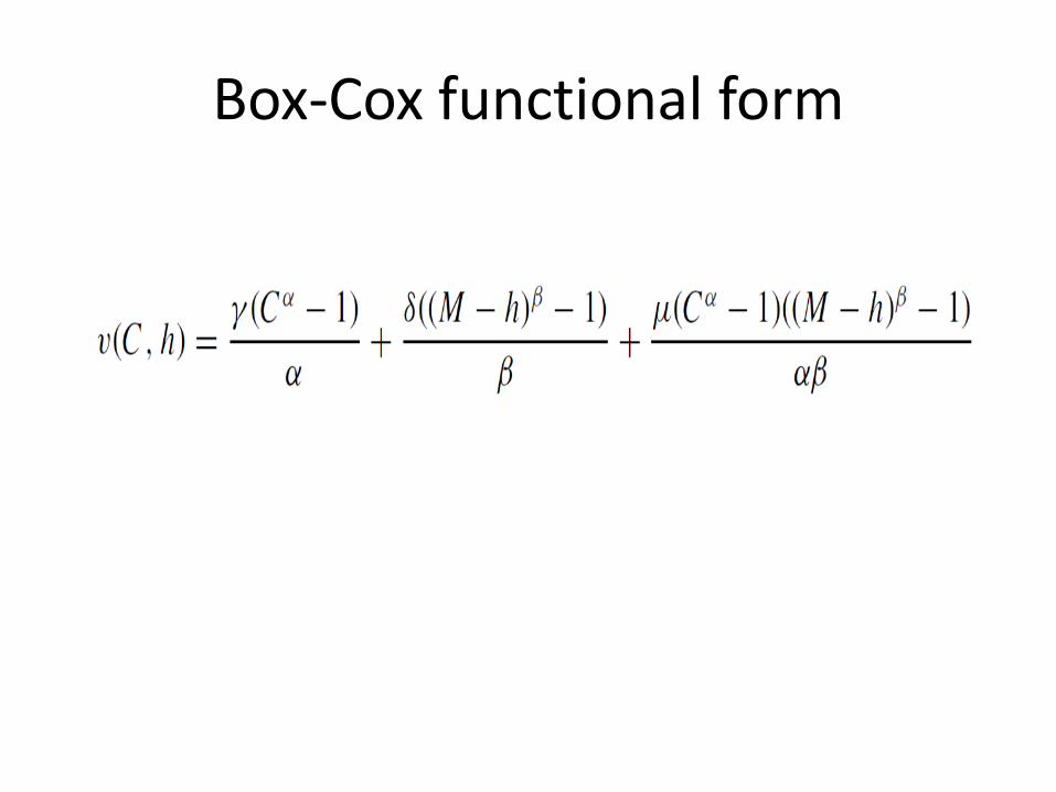
Box-Cox functional form

Which data are used?
• Information about working hours from Arbeidskraftundersøkelsen (AKU)
• In combination of income data from Income statistics
• Useful to have a tax-benefit calculator
– Calculate taxes in each discrete choice

Example of estimation results (from Thoresen and Vattø, 2015)
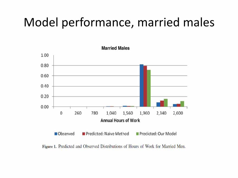
Model performance, married males
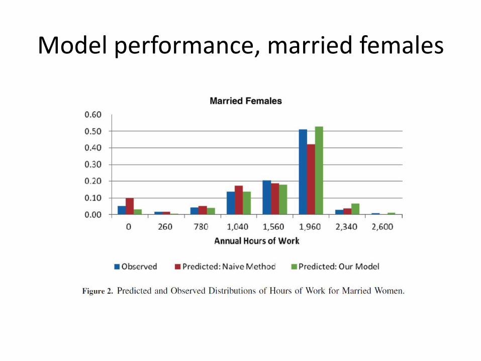
Model performance, married females

Model performance, disposable income

Summary
• Hausman approach complicated to use in practice – But marginal criteria appealing
• Conventional discrete choice model (van Soest) popular among practitioners
• Job choice model provides more realistic decision model
• LOTTE-Arbeid (Statistics Norway) uses job choice model
• Static models − policy issues may have important dynamic effects


