Lagrangian Thermodynamics of Heat Transfer in Systems ... · Lagrangian Thermodynamics of Heat...

Lagrangian Thermodynamics of Heat

Transfer in Systems Including Fluid Motior2

M. A. BIOT”

Cornell Aeronautical Laboratory, Inc.

Summary

The Lagrangian thermodynamic equations of irreversible processes are extended to convective heat transfer. This generalization provides equations for the unified analysis of transient heat flow in complex systems comprising solid structures and moving fluids in either laminar or turbulent flow. The concept of a surface-heat-transfer coefficient is eliminated from the formulation. The theory is developed along two different lines. In one approach a new concept referred to as the “trailing function” is introduced. It represents the surface-heat-transfer properties and may be evaluated by quite simple but remarkably accurate variational procedures. The method of “associated fields” is also generalized to convective phenomena. The second line of approach extends to convective heat transfer the thermodynamic concept of entropy production for both laminar and turbulent flow. The theory amounts to an extension of the thermodynamics of irreversible processes to systems for which Onsager’s relations are not valid.

(1) Introduction

I N HEAT-FLOW PROBLEMS of solid structures which are in contact with moving fluid at the boundaries, it has

been customary to carry out the analysis by introducing the concept of a surface-heat-transfer coefficient. How- ever, the general inadequacy of this concept in connec- tion with boundary-layer heat transfer has been demonstrated.’ The need, therefore, arises for a general theory which does not require the use of such a concept.

It turns out that the Lagrangian methods of heat- transfer analysis are very well suited for this purpose. They were presented in Refs. 2 to 4 and are based on principles of nonequilibrium thermodynamics.

It is possible to develop the theory along two different lines.

One way is to represent the surface heat transfer by means of a new concept referred to here as a trailing function. It represents the surface temperature distribution due to a unit rate of heat injection in the moving fluid at a point PO of the surface while thermal insulation is maintained elsewhere. It is essentially in the nature of a two-point influence function represent- ing the temperature at point P due to a heat injection at PO. The trailing function yields a complete descrip- tion of the heat-transfer properties if we assume that the principles of superposition are valid. It is applicable to laminar as well as turbulent flow. In the context

Received April 13, 1961. Revised and received November 30, 1961.

t This work was performed as part of a Cornell Aeronautical Laboratory internal research project. This paper first appeared as C.A.L. report No. SA-987-S-11, March 1961.

+ Consultant.

of linearized perturbation theory we may look upon the local heat injection as producing temperature changes which result not only from the heat flow but also from the variations of the velocity field, the turbulence, and other factors, such as viscosity, thermal conductivity, and physical chemical equilibrium.

Transition from laminar to turbulent flow originating in the heat transfer itself does not obey the principle of superposition. A method for analyzing this case is briefly discussed in Section (4).

The concept of a trailing function is introduced and discussed in Section (2). In Section (3) it is shown that remarkably accurate variational methqds may be used for its evaluation. In Section (4) the general Lagran- gian equations are formulated for the transient-heat- flow analysis of general systems which include moving fluids. The reciprocity properties known as Onsager’s relations5 are not verified for these equations. This is a reflection of the fact that the present formulation con- siders a perturbation from an initial state which is one of motion instead of one of static equilibrium. From a mathematical viewpoint, this is equivalent to stating that the problem is not self-adjoint.

Section (5) deals with the associated-field method which was introduced and developed earlier3 for the purpose of simplifying the formulation of two- and three-dimensional problems. It is shown that this method is applicable to systems including convective heat transfer and that the associated field itself satisfies a “reverse flow” theorem.

A second and quite different line of approach is followed by a direct extension of the Lagran- gian thermodynamics to convective flow. Along this line an important result has recently been obtained by Nigam and Agrawal,6 who derived a formal expression for the dissipation function in the context of laminar flow. On the other hand, it is possible to show that the thermodynamic definitions of thermal potential, entropy production, and thermal force are valid for the analysis of heat transfer by convection and lead directly to a Lagrangian formulation. These thermodynamic considerations yield a dissipation function which is different from the one introduced by Nigam and Agrawal, but coincides with it in some particular cases. These results are discussed in Section (6) and are further generalized to include the case of unsteady turbulent flow. The concept of entropy production and dissipati& function is applicable to turbulent diffusion. Hence, the same Lagrangian equations govern the heat flow in complex systems which include both solids

Reprinted from JOURNAL OF THE AEROSPACE SCIENCES Copyright, 1962, by the Institute of the Aerospace Sciences and reprinted by permission of the copyright owner

MAY, 1962 VOLUME~~, No. 5

and moving fluids in laminar or turbuIent flow. As a consequence, it becomes possible to carry out a unified analysis of such systems as a whole without explicit reference to any surface-heat-transfer properties.

The thermodynamic implications of this result are also discussed. In particular, it is pointed out that the Lagrangian equations are applicable to systems for which the Onsager relations are not valid. This leads to generalizations which reach far beyond the narrow field of heat transfer and will be the subject of later publications.

We have also called attention to a generally mis- understood aspect of the theory as regards the heat generated by the dissipation itself.

Results presented here were briefly outlined earlier in Ref. 11.

(2) Introduction of the Concept of “Trailing Function”

Consider a solid boundary in contact with a moving fluid. The flow may be laminar or turbulent. In the latter case fluctuations of the velocity and temperature occur around certain average values. It is these average values which we shall refer to hereafter as the temperature and velocity fields. For the time being let us assume that we are dealing with a steady-state condition. This means that the average values of the temperature and velocity at any given point are independent of time. If there is no heat transfer from the solid to the fluid, the temperature of the fluid at the boundary is the so-called adiabatic temperature. The adiabatic temperature O,(P) at a point P of the surface depends on the location of P and is deter-mined by the mechanics and thermodynamic of the flow. This is a very general concept which has been used extensively and includes a great variety of phenomena such as convection, thermal conduction, turbulent diffusion, heat generated by laminar and turbulent friction, radia- tion, and chemical effects.

If the temperature distribution at the wall is not O,(P) but B(P), a heat transfer occurs. This heat transfer may be associated with only a slight variation in the flow pattern, in which case it is reasonable to assume a linear dependence between the heat transfer and the temperature variation. We may write this dependence in the form of a linear integral relation,

B(P) = c&(P) - J I&(P’)r(P, P’)dS,J (2.1) s

The quantity fin(P’) is the heat flowing into the solid per unit time and unit area at point P’. The element of area at point P’ is d&r. The function r(P, P’) con- stitutes a generalization of the heat-transfer resis tivity-i.e., of the inverse of the surface-heat-transfer coefficient. In order to illustrate its physical significance, let us introduce the surface Dirac function 6(Po, P’). This function is such that

FIG. 1. Isothermal contours for trailing function with heat injection at point 0 (schematic).

and

~(Po, P’) = 0 for PO # P’ (2.2)

S ~(Po, P’)d.S,, = 1 s

(2.3)

If we put -&(P’) = 6(Po, P’) (2.4)

it represents a concentrated injection of a unit’s amounts of heat per unit time at point PO into the fluid. Intro-

ducing this expression into the integral relation (2.1) we find

B(P) - &Z(P) = r(P, PO) (2.5)

This yields the physical interpretation of the function r(P, PO) as the surface temperature increment at P due to a unit rate of concentrated heat injection into the fluid at PO. An example of a trailing function is shown in Fig. 1, where point PO is located at 0 and the isothermal contours correspond to constant values of r. It can be said that the heat injection produces a temperature trail downstream from the point of injection. Therefore, we shall refer to the function r(P, PO) as the “trailing function.” We must remember that this definition implies that there is no heat flow through the boundary except at point PO.

Attention is called to the important property that for

a moving fluid the trailing function is not symmetric- i.e.,

r(P, P’) # r(P’, P) (2.6)

Until now we have assumed the temperature to be stationary. In the case of unsteady heat flow the trailing function should, strictly speaking, contain the time explicitly even for steady fluid motion. This dependence on time would then represent a time lag because of the finite velocity of convection. However, the numerical discussion which was given in Ref. 1 indicates that the time-dependent term in the heat-flow equations may generally be discarded. Therefore, in most practical problems the time scale of heat conduction and of fluid velocities is such that the time lag may be neglected. The trailing function r(P, P’) may then be considered to represent an instantaneous steady state. The same considerations may be applied to the case where the fluid motion is unsteady. In this case the trailing function which again results from a succes- sion of instantaneous steady states is a function of the time t and Eq. (2.5) is replaced by

B(P) - f?,(P) = r(P, P’, t) (2.7) The dependence of the trailing function on time is de- termined by the time-dependent velocity pattern of the

569

570 JOURNAL OF THE AEROSPACE SCIENCES-MAY 1962

fluid or, more precisely, by the linear perturbation of the combined fluid dynamics and thermodynamics of the unsteady flow.

Attention is called to the extreme generality of the concept of a trailing function within the framework of linear perturbation. The unperturbed adiabatic temperature field includes the effect of heat generation in the fluid by the motion itself because of the viscosity. The perturbation in the temperature field produced by a heat injection at the wall is theoretically the result of very complex interaction between a number of variables, which include the change in velocity field, viscosity, and diffusivity. From the analytical viewpoint this involves the solution of the linearized perturbation problem for the coupled Navier-Stokes and thermal-chemical field problems.

The analytical difficulties are enormously simplified if the variations of velocity field, viscosity, and diffusivity are neglected. This procedure is justified in a large category of problems, since-in the case there is no variation of the heat generation in the fluid-the perturbation of the temperature field is governed by equations of the type considered in Ref. 1, which do not involve heat sources in the field.

Problems where the heat transfer causes a transition from laminar to turbulent flow are, of course, not open to treatment by perturbation techniques. A possible procedure for this case will be discussed in Section (4).

(3) Evaluation of the Trailing Function by Variational Methods

We shall derive some simple examples of the trailing function for a homogeneous incompressible fluid. Let us take first the case of two-dimensional flow. The x axis is on the solid surface, and the two-dimensional field is in the x, y plane and independent of the z coordinate. Heat is injected into the fluid at a unit rate per unit length of the z coordinate.

This is equivalent to stating that the boundary condition for the temperature field at the wall is

- K@e/~Y) lpo = w (3.1)

where k is the thermal conductivity of the fluid and S(x) a Dirac function. According to the conduction analogy, l* 6l l1 Eq. (3.1) is replaced by

- [k’(bB’/dy)]ll=o = 6(t) (3.2)

where k’ = K = k/c is the thermal conductivity of the analog model. In addition, we introduce an analog heat capacity c’, and an analog temperature 8’ = 60.

Eq. (3.2) may be interpreted as stating that a unit amount of heat per unit area is injected into a wall at the time t = 0 and allowed to diffuse freely in the y direction normal to the surface. In the particular case of constant value of the thermal conductivity k’ and heat capacity c’ per unit volume, the exact solution of this problem is well known. The temperature obeys a Gaussian distribution

0’ = (l/c’)mexp [-c’yz/(4k’t)] (3.3)

Note the property that

S m

cWdy = 1 (3.4) 0

which corresponds to the condition that a unit amount of heat has been injected. The wall temperature is

0 20 ‘ = 2/ l/(&k’t) (3.5)

Replacing the variables corresponding to the analogy- viz., replacing k’ by K, c’ by U, 0’ by ctJ, and t by x, we find

0, = l/&lJkcx (3.6)

This represents the trailing function for injection of heat at the origin x = 0. If points P and P’ are located at the coordinates x and E, the trailing function for this case is

r(P, P’) = l/&r Ukc(x - s$) (3.7)

The solution for the trailing function may be obtained by a variational procedure in the conduction analogy. Let us assume that the temperature due to a unit heat injection is approximated by

8’ = e,' [i - (y/g) 1 (3.3)

The condition that the total heat content is unity is

PQ

J- c'e'dy = 1 0 (3.9)

or 8 u) ’ = 3/(2c’q)

There is only one unknown p. The thermal potential is

v = (3/5) [l/(c’a) 1 (3.10)

The heat flow is

H = 1 - (3/2)(~/q)

The dissipation function is

D=& S Q

if2 dy 0

+ i/2(y3/q3) (3.11)

3 1 42 =__- 35k’ q

(3.12)

The thermal force is zero, since the wall is assumed to be insulated. Hence, the Lagrangian equation is

(aIrlap) + @D/@) = 0 (3.13)

or

2@ = 7k’/c’ (3.14)

By integration

p = l/7(k’/c’)t (3.15)

Substituting in Eq. (3.9), we find the wall temperature

1

em’ = 1/(28/9)c’k’t

Comparing with the exact value [Eq. (3.5)] we see that

the constant & = 1.772 is replaced by 2/2s/9 =

LAGRANGIAN THERMODYNAMICS 571

1.765. Hence, the error of the variational method is of the order of slide-rule accuracy. With the trailing function (3.7) the integral (2.1) giving the wall temperature due to an arbitrary distribution of heat injection becomes

If the field is approximately two-dimensional, the wall temperature 8(x, z) varies slowly in the direction z per- pendicular to the flow. We may use the same one- dimensional trailing function and write the approxima- tion

S 5

B(x, 2) = e(x,z) - iL(F,z)dE -

drUck(x - [) (3.17)

If the temperature variations in directions perpendicu- lar to the flow are very rapid, we must consider a two- dimensional trailing function.

Thus function could be measured or evaluated by analytical methods. Under the particular assumption that no change occurs on the velocity field or in the internal heat generation, the temperature field is governed by the equation

This equation follows immediately from results discussed previously.’ The parameter A is the sum of the thermal diffusivity K = k/c and the turbulent diffusivity -i.e.,

A = K + r = (k/c) + e (3.19)

The flow is assumed to be in the x direction with a velocity distribution V(y). The total diffusivity A may be a function of y and z.

The injection of-a unit rate of heat flow at the origin is expressed by the condition

- [k(b~/~y) ly=o = GM4 (3.20)

The corresponding conduction analogy is expressed by the equation

c’ g = ; (6’:) + ; (k’$) (3.21)

This expresses the transient heat conduction in the half plane y, z (y > 0). The correspondence of variables in the analogy is

t = x, c’ = U(y), k’ = A (y, z), 0’ = co (3.22)

In the analogy the boundary condition (3.20) becomes

- [k’(bB’/by) Iv=,, = 6(@(z) (3.23)

This expresses the instantaneous injection of a unit amount of heat at the origin, and when t = 0, in the half plane. If we assume a uniform laminar flow of constant velocity U, we must solve the time-dependent analogy for c’ and k’ constant. The solution of this problem is known.7 The temperature is

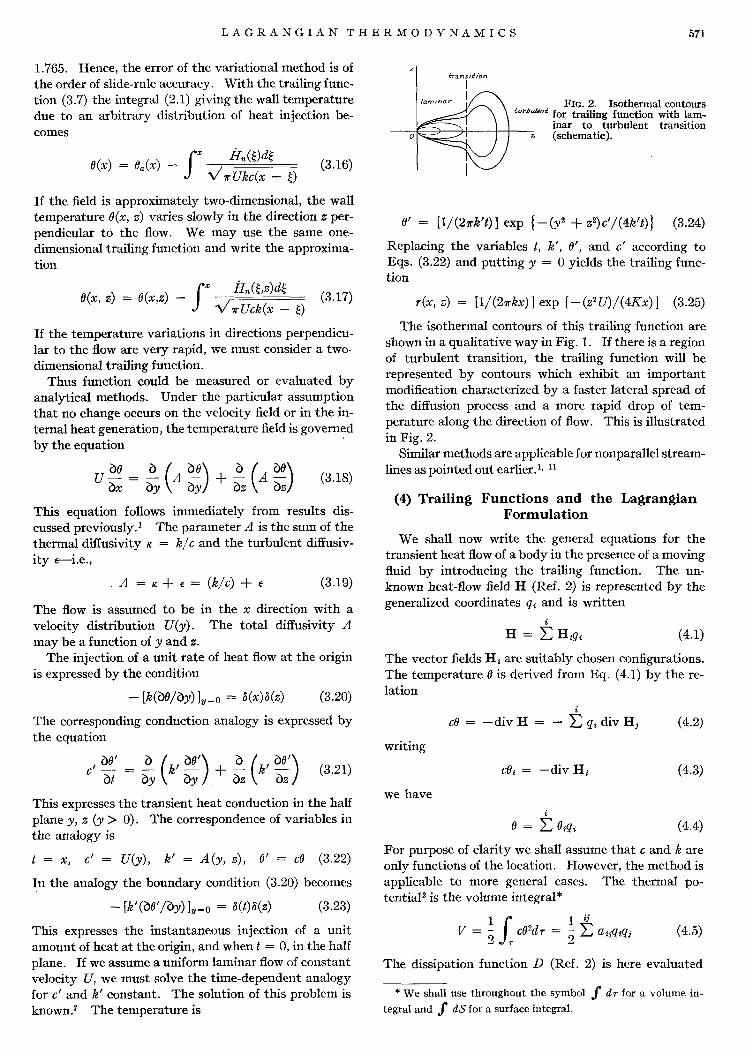
FIG. 2. Isothermal contours for trailing function with laminar to turbulent transition (schematic).

0’ = [1/(2?rk’t)] exp {-(yz + z2)d/(4k’t)j (3.24)

Replacing the variables t, k’, 0’, and c’ according to Eqs. (3.22) and putting y = 0 yields the trailing function

r(x, z) = [1/(2?rkx)] exp [ - (z2U)/(4Kx)] (3.25)

The isothermal contours of this trailing function are shown in a qualitative way in Fig. 1. If there is a region of turbulent transition, the trailing function will be represented by contours which exhibit an important modification characterized by a faster lateral spread of the diffusion process and a more rapid drop of temperature along the direction of flow. This is illustrated in Fig. 2.

Similar methods are applicable for nonparallel stream- lines as pointed out earlier.‘, l1

(4) Trailing Functions and the Lagrangian Formulation

We shall now write the general equations for the transient heat flow of a body in the presence of a moving fluid by introducing the trailing function. The unknown heat-flow field H (Ref. 2) is represented by the generalized coordinates qr and is written

H = 5 Hip,

The vector fields Hi are suitably chosen configurations. The temperature 13 is derived from Eq. (4.1) by the relation

ce = -divH = - kqrdivHj (4.2)

writing

c& = -div H, (4.3)

we have

e = 2 Oiqi (4.4)

For purpose of clarity we shall assume that c and k are only functions of the location. However, the method is applicable to more general cases. The thermal po- tentia12 is the volume integral*

S Ce2dT = 5 2 afjqiqj (4.5) 7

The dissipation function D (Ref. 2) is here evaluated

* We shall use throughout the symbol $ dr for a volume in-

tegral and s dS for a surface integral.


for the solid alone without including any surface-heat- transfer dissipation. We write

The thermal force2 is defined by the temperature distribution at the solid boundary. If we denote by 19(p) the unknown temperature at point P of the solid boundary, the generalized force corresponding to qi is the surface integral

Qi’ = s, W)

where H,(P) indicates the

@L(P) dS

b¶c p (4.7)

normal component of H taken positively inward at point P. The integral is extended to the boundary S of the solid, and dSp is the element of area at point P of this boundary. Con- sider Eq. (2.1)

B(P) = t&(P) - s

&(P’)r(P,P’)d& (4.8) s

where dS,p is the element of area at point P’. Sub- stituting in Eq. (4.7) yields the expression of the generalized thermal force

Qt’ = - j-L? &(P’)r(P,P’)dSpdSpr + a

S 0 (P) dHn(p) dS ~ a P (4.9)

S &li

From Eq. (4.1) we may write

H,(P) = ii Hin(P)qi

X&(P) = 2 Hila(P)4c

(4.10)

with Hi, (P) equal to the normal component of HI at point P taken positively inward. Substituting Eq. (4.10) in Eq. (4.9) we find

with

Qi’ = - i ci& + Qi (4.11)

cij = ss H,,(P)H,,(P’)r(P,P’)dSpdSp~ (4.12) s s

Qi = S, ea(P)H,n(P)dSp (4.13)

We now apply the general Lagrangian equations2 to the thermal system. These equations are

(bV/%a) + (a)/@3 = Qi’ (4.14)

Substituting expressions (4.5)) (4.6)) and (4.11) in these equation yields

2 aijqj + k (baj + ct,)aj = Qi (4.15)

The coefficients al5 and bar in these equations are symmetric- i.e.,

% = aji, b,, = bjl (4.16)

However, in general, for the case of a moving fluid

cy # Gr (4.17)

As seen from Eq. (4.12) the nonsymmetry of cij is due to the nonsymmetry of the trailing function (2.6). The inequality (4.17) indicates that if we consider the thermal system from the thermodynamic viewpoint, On- sager’s relations do not apply. This is, of course, due to the fact that we are dealing with the thermal perturbation of a system which is not in equilibrium in its initial state but is already in motion. In other words, we are dealing with the perturbation of a thermodynamic system in the vicinity of a nonequilibrium state.

The fluid motion at the boundary may be a function of time, in which case the trailing function is of the form of Eq. (2.7). It is a function of time as well as of the coefficients cij. We write

c%,(t) = ss

H,,(P)H,,(P’)r(P,P’,t)dSpdSpt (4.18) s s

We must then solve the differential Eqs. (4.15) with coefficients which are functions of time. These equations generalize to a moving fluid the case of time- dependent boundary heat transfer already considered previously.

We have mentioned the possibility of using the present equations to analyze problems where the heat transfer induces a laminar-to-turbulent transition or strongly influences the transition point. One possible method which suggests itself naturally is the trial-and-error procedure. We may assume a tentative position for the transition line of the trailing function illustrated in Fig. 2. The temperatures are then computed, and a new transition point is derived from the result. The procedure is repeated until the calculated temperatures correspond approximately to the location of the transition point.

(5) Associated Flow Fields Generalized to Convective Heat Transfer

The equations of Section (4) contain unknowns which we have referred to as ignorable.” 3 They correspond to flow fields which are divergence-free and, therefore, do not affect the temperature field. If we are not interested in the heat flow but only in the temperature distribution, it is of considerable interest to eliminate these ignorable coordinates from the problem right at the start. Methods to accomplish this were briefly indicated in Ref. 2 and developed in considerably more detail in Ref. 3. The method introduces the concept of the associated field by which a temperature field, depending on a certain number of generalized coordinates, is associated with a corresponding vector flow field. This associated field is derived from the corresponding temperature configuration by methods developed in Ref. 3, including variational techniques.

We will show here that this associated field method may be extended to problems of heat flow in the presence of a moving fluid. Let us represent the heat flow field as


H=Hg+F

where F is the divergence-free part

div F = 0

Let us represent the temperature field by

(5.1)

(5.2)

e = 2 ecqa (5.3)

and the flow field by

H = 2 &pi + 2 Fjpi

in which the two terms of Eq. (5.1) are

(5.4)

F = 2 Fifj (5.5)

The temperature is related to the flow field by relation (4.2), and F represents the divergence-free part. Hence, the equations

div oi = --cBc (5.6)

div Fj = 0 (5.7)

The coordinates fj represent the ignorable coordinates. Eq. (5.6) is, of course, not sufficient to determine the vector field Oa once the temperature configuration 0% has been chosen. However, this may be done if we im- pose the extra condition that the coordinates qr and fj be uncoupled in the final equations.

Since 0 is independent of fj, these coordinates do not appear in the thermal potential [Eq. (4.5)]. The coupling can only occur through the dissipation function and the term Qt'.

The dissipation function in the solid is written

(58

The thermal force Qt’, as derived from Eq. (4.9), is

Qi' = - 5 ciz4z - i cij_!i + ~s~.(P)@i,(PW~

(5.9)

with

ciz = ss ean(P>ezn(P’>r(P,p’>dSpds,, s s

(5.10)

The subscript n, as above, indicates the normal components of the vectors OS and F, with a positive inward direction. There is a similar expression Qj’ correspond-

ing to the ignorable coordinates fi. The differential equations separate into two groups:

@V/d& + (bD/bqi) = Qi’; dD/bfj = Qj’ (5.11)

The first group of Eqs. (5.11) may be written

(5.12)

The coefficients are given by Eqs. (5.10) and by

UfZ = S 7

ceiez dr,

bij = S 7

@@z dr

(5.13)

We also define a thermal force Qj associated with the adiabatic wall temperature e=(P),

Qi = ~B,oB,,(P)dS, (5.14) s

The coordinates f, are coupled to the coordinates p1 in equations through the coefficients bti and I+. The question is to chose the fields Of in such a way that these coupling terms vanish-i.e., such that

bi, + ccj = 0 (5.15)

To this effect we put

O( = -k grad #( (5.16)

This involves a flow potential tic which was introduced in Refs. 2 and 3. By Eq. (5.6) we find a relation between the flow potential IJ$ and the temperature field 8 0

div k grad 9% = c& (5.17)

The physical significance of this equation is obtained by considering tii to represent a steady-state temperature produced in the thermal system by a heat-sink distribution c&.

The sink distribution cei does not define the temperature uniquely unless we add a boundary condition. We will now show that this missing boundary condition is furnished by the condition [Eq. (5.15)] that the coordinates pc and ft be uncoupled. Let us substitute in expression (5.10) and (5.13) for bij and cij the flow potential, using relation (5.16). We find

(P)Fi,(P’)r(P,P’)dSpdSp, (5.18)

In this equation grad, indicates the normal component of the gradient chosen positively outward. We may in- tegrate the volume integral by parts. Because the divergence of the field Fj is assumed to be zero, we find

Eq. (5.18) then becomes a surface integral


bi, + cij = s A ,(P’) Fj,(P’)dSP (5.20) S

with

A,(P) = S K grad, vW'bG'J"Wp + VW"> S

(5.21)

For condition (5.15) to be verified for any divergence- free field Fjn we must have

A,(P) = 0 (5.22)

This furnishes the boundary condition required to determine the flow potential $c corresponding to the temperature Bc. The associated flow fields are defined from Eq. (5.16). Under these conditions the ignorable coordinates fj do not appear in Eqs. (5.12). The boundary condition (5.22) may be written in a different form which brings out its physical significance. We may in- terchange P and P’, since this is simply a change of notation. Condition (5.22) then becomes

#,(P) = - Jsk grad, $,(P’)r(P’,P)dS,/ (5.23)

Furthermore,

K grad, #,(P’) = &(P’> (5.24)

represents the rate of heat inflow at point P’ where a temperature field $( exists in the solid. Hence, the boundary condition

up> = - S I?,(P’)r(P’,P)d.s,t (5.25) S

Comparing with Eq. (2.1), we see that #( is a temperature field satisfying Eq. (5.17) in the solid, and a boundary condition such that the adiabatic temperature is zero and the trailing function is r(P’,P). Note that this is not the trailing function of the actual fluid but that obtained by interchanging points P and P’.

Reverse-Flow Theorem

It is possible to state a reverse-flow theorem for the trailing function in the case of incompressible flow with constant heat capacity. The proof of this theorem is given in Appendix I. It states that if r(P,P’) is the trailing function associated with a given fluid velocity field and r(P,P’) the trailing function associated with the field obtained by reversing the sign of the velocities, we have the property

r(P,P’) = r(P’,P) (5.26)

The total diffusivity field A is assumed to be the same in both cases.

By applying relation (5.26) it is possible to write the boundary condition (5.25) as

#g(P) = - s, &(P’)ii(P,P’)dS,~ (5.27)

Hence, when the reverse-flow theorem is applicable, the associated field is the steady-state flow produced by a

distribution of sinks cer in the solid, while the velocity field of the fluid at the boundaries is reversed.

Variational Principle for the Associated Field

The associated field O1 may be evaluated directly for a given distribution et by a variational principle stated as follows

S e,,(P’)r(P’,P)dS,~ = 0 (5.28) S

This expression is made to vanish under the constraint (5.6). The principle is a generalization of a similar one developed in Section 4 of Ref. 3 for the case of a surface- heat-transfer coefficient. It is immediately derived by the same method.

(6) The Generalized Lagrangian Thermodynamics of Convective Heat Transfer

Consider the temperature field in an incompressible fluid. The temperature 8 satisfies the equation

div (k grad 0) = c(be/bt) + cuograd 8 (6.1)

The fluid velocity is denoted by U. This equation is applicable to both solid and fluid. In the solid the thermal conductivity k(x, y, z, 0) and the heat capacity c(x, y, z, 0) per unit volume may be functions of the location and the temperature, while in the fluid k(8) and c(0) are functions only of the temperature.

We have shown that the Lagrangian equations

@IrlW + (do/%&) = Q1 (6.2)

govern the conductive heat transfer, and by introduction of the trailing function are also applicable to systems including a moving fluid.

Let us move one step further and examine the possibility of deriving the same Lagrangian Eqs. (6.2) for convective heat transfer governed by Eqs. (6.1). The question has already been considered by Nigam and Agrawal,6 who introduced a formal definition of the dissipation function. We will show that it is possible to use a different definition of the dissipation function based on the thermodynamic concept of entropy production. Furthermore, the result may be extended to systems which are less restricted than Eqs. (6.1), such as those including unsteady turbulent flow.

Let us first consider the more restricted case governed by Eqs. (6.1). The heat-flow vector H is related to the temperature by the constraint equation L9

h= S cd0 = - div H (6.3)

and the thermal potential is

s s 9

V= dr cede 7

(6.5)

These equations are the same as those introduced pre-


viously by this writer.2 The dissipation function, however, is different and is defined by the relation

D=f s

.; (B - hU)2& (6.5)

The volume integrals over 7 are extended to the complete system composed of the solid components and the moving fluids. The thermal force Qi is also defined as previously by the virtual work of the temperature applied at the fluid or solid boundaries.

The proof of Eq. (6.2), using the above definition, is developed in Appendix II for the more general case of turbulent flow. This result leads immediately to some very illuminating and fundamental considerations with respect to the thermodynamics of irreversible processes. The link with thermodynamics is brought out by using the law of heat conduction in the form

-kgradB = l!t - hu (6.6)

Substituting this expression into the dissipation function (6.5), we derive

L&i S k (grad e)2 d7 (6.7) 7

Let us assume that the absolute fluid temperature is 8 + T,, where T, is a reference temperature and 0 represents a temperature deviation which is small relative to T,. As shown by Meixner,s the rate of entropy production per unit volume is

R = (k/TT2)(grad e)2 (6.3)

Hence, the expression 2Tr2D represents the rate of entropy production in the volume of fluid. Eq. (6.8) was also discussed by this writer in the more general context of thermodynamics and thermoelasticity [Ref. 9, Eq. (7.19) 1. Attention is called to the omission of the com- mon factor l/T, in the definition of the quantities V, D, and Q for problems concerned exclusively with heat flow.

The important fact emerging from these remarks is the generality of the Lagrangian Eqs. (6.2). We are dealing here with a system whose initial unperturbed state is not a state of thermodynamic equilibrium but a state of motion. The Lagrangian equations are valid for the perturbation of this nonequilibrium process provided the function D is defined as proportional to the increment of entropy production due to the perturbation.

The reader will note that this example involves principles which are more general than those of the thermodynamics of irreversible processes as they stand at this time, since the latter concerns systems which are perturbed in the vicinity of an equilibrium state.

Moreover, it can be seen that the Onsager reciprocity relations will not be verified when the dissipation function is defined by,the more general Eq. (6.5). For example, if the field is expressed linearly in terms of generalized coordinates, the dissipation function will be of the form

with

bij’ # b,r’ (6.10)

Hence, the matrices in the differential Eqs. (6.2) will not be symmetric. The nonapplicability of the Onsager reciprocity relations for systems including convection has already been studied in Section (4) by an entirely different, more general procedure, using the concept of a trailing function.

Another point of considerable interest lies in the possibility of generalizing the Lagrangian approach to the case of turbulent heat transfer. The differential equations for the temperature field become

div [CA grad f?] = c(be/dt) + cuagrad e (6.11)

The parameter A@, y, z, t, 0) is the total diffusivity as defined above [Eq. (3.19)]. It may be a function of the location, the time, and the temperature. The mean velocity field is denoted by u. The Lagrangian Eqs. (6.2) are then applicable to heat-transfer problems governed by Eqs. (6.11)) provided the dissipation function is defined as

DE; S 7; (H - hu)2 dr (6.12)

This expression is proportional to a quantity which includes the entropy production associated with turbulent diffusion. The analytical derivation of this result is given in Appendix II along with its generalization to anisotropic conductivity and nonisotropic turbulence.

An important consequence of these results is the possibility of applying the Lagrangian Eqs. (6.2) to composite systems made up of solids in the presence of unsteady fluid flow under conditions of either laminar or turbulent flow. The solid part is then represented by putting u = 0 in the equations in the solid region.

By this token a unified analysis can be made of transient heat flow in the combined fluid-solid system. We should also draw attention to a sometimes mis- understood point regarding the additional term due to the heat generated by the fluid friction and, more generally, by the dissipation itself. The particular nature of this effect was discussed by the writer in con- nection with thermoelasticity.rO When introduced in the equations, it must be considered as a given source external to the system and, therefore, independent of the coordinates subject to the variational process.

As pointed out in Ref. 3, inclusion of a given source is readily accomplished by writing the constraint Eq. (6.3) as

h = -divH+ S t

wdt

where w is the rate of heat generation per unit volume considered as a given function of time and location. In the more general thermodynamics w is a term of the second order relative to the unknown variables. It may, therefore, be neglected without loss of generality


in linear theories such as those for viscoelasticity and thermoelasticity summarized in Ref. 10.

Appendix I

Reverse Flow Theorem

Consider a homogeneous and incompressible fluid in steady laminar or turbulent flow. The temperature field satisfies the equation

div(ca grad 0) = cu * grad 0 (1.1)

The total diffusivity may be a function of the coordinates, and c is a constant. The temperature 6 in the same fluid where we reverse the velocity field without changing the diffusivity is governed by

div (CA grad 4) = -cu. grad 8 (1.2)

From these equations we derive

0 div (CA grad 0) - 0 div (CA grad 0) =

cu. (0 grad 0 + e grad 4) (1.3)

Using the condition of incompressibility this may be written

div(ctltI grad e - CAB grad 8 + ce&) = 0 (1.4)

The volume integral of this expression may be trans- formed into a surface integral over the boundary S, leading to the equation

S (CAB grad, e - cA0 grad, 4 - c&,)dS = 0 (1.5) S

where grad, e and un designate the normal components of the gradient and the velocity, chosen positive outward. If we consider part of the boundary S to be made of the interface of solid and fluid, while the re- maining part is far enough removed so that 0 vanishes, then either e or u, vanishes at the boundary, and Eq. (1.5) is written

S (CAB grad, 0 - c&3 grad, J)dX = 0 (1.6) W

where the integral extends over the fluid-solid interface W.

Assume now that the field 8 is produced by a unit rate of concentrated heat injection at the point P’. In this case we may write

CA grad,, 0 = 6(P,P’) (1.7)

where 6 is a Dirac function, and the value of 8 at the surface represents the corresponding trailing function

e = Q,P’> (1.3)

Similarly, 0 may be chosen to represent the field due to concentrated injection at point P is the reverse flow. Then

CA grad, 8 = 6(P,P”); Jj = f(P,P”) (1.9)

where v is the trailing function in the reverse flow. With these functions, Eq. (1.6) becomes

S s [r(P,P”)G(P,P’) - ,(P,P’)b(P,P”)]dS, = 0 (1.10)

or

v(P’,PK) = T(PK,P’) (1.11)

This establishes that the trailing function for reverse flow is obtained by interchanging the points in the trailing function for direct flow.

Appendix II

We shall establish the validity of the Lagrangian Eqs. (6.2) for a system including unsteady turbulent flow. Consider the average heat-flow field

H = H(qlqz . . . qn 2 y z t) (11.1)

as a parametric function of generalized coordinates qf. The field is subject to variations which are virtual and expressed by

(11.2)

The average temperature 0 is related to H by the relation

s

9 h= cde = -div H (11.3)

0

In this expression c is the heat capacity per unit volume. In the solid it may be a function c(z, y, z, 0) of the location and the temperature, while in the fluid it is a function c(e) of the temperature alone. It is important to note that this equation which physically expresses conservation of energy is intended here as a constraint,. It is to be verified not only by the final solution of the problem but also by the variations themselves. Hence, we also write

sh = cse = -div 6H (11.4)

Introduce the variational invariants

6V = S

de dr 7 6A = S $ (ti - hu)GH dr

(11.5)

In these expressions the total time derivative of the heat flow is

(11.6)

The total diffusivity due to thermal and turbulent diffusion may be a function of the coordinates, the time and the temperature

A = A (2, Y, 2, t, 0) (11.7)

Using the first of Eqs. (11.5) and integrating by parts yields

6V = S 6H. grad t?d r + S Bn.6H dX (11.8) * s


The law of heat conduction and diffusion is expressed by

CA grad 0 + $I - hu = 0 (11.9)

Hence, adding Eqs. (11.5), we derive

6V + 6A = S on.6H dS (11.10) s

The unit normal (positive inward) at the boundary S of the volume r is denoted by n.

The variational principle [Eq. (ILlO)] may be written in an alternate way by introducing the variations 6q instead of 6H. We write

6H = kFaq, t

(II.11)

Also, from Eq. (IT.6),

&i/b& = aH/dq, (11.12)

Hence, we derive the alternate expressions

with

s s 8 V= dr

7 0 &de; D=; S .& (iI - hQ d7

(II. 14)

In addition, we may write

S On*6H dS = 2 Q&t (11.15) s

with

(11.16)

The surface integrals are extended to the boundary S of r. Substituting Eqs. (11.13) and (II.15) into the variational principle [Eq. (II.lO)] leads to the La- grangian equation

@V/W + WI&k) = Qi (11.17)

We have thus extended the validity of these equations to unsteady turbulent heat transfer. Extension

of these results to systems with anisotropic conduction and nonisotropic turbulence is immediate by applying Eq. (3.15) of Ref. 2 for the dissipation function. In this case it becomes

. . D=& S Aij (I?i - hui)(fij - huj) d7 (11.18)

7

In this expression AU are the elements of the inverse matrix of CAu = kij + Clij where k,, represent thermal conduction and lij is the nonisotropic turbulent diffusivity tensor.

The above derivation is also valid if the heat generated by the fluid friction is included. Both generalizations are discussed in Section (6).

References

1 Biot, M. A., Fundamentals of Boundary Layer Heat Transfer with Streamwise Temperature Variations, Cornell Aero. Lab., Rep. No. SA-987-S-10, March 1961 (Journal of the Aerospace Sciences, this issue).

2 Biot, M. A., New Methods in Heat Flow Analysis with Ap- #Gutions to Flight Structures, Journal of the Aeronautical Sciences Vol. 24, No. 22, 1957.

3 Biot, M. A., Further Development of New Methods in Heat Flow Analysis, Journal of the Aero/Space Sciences, Vol. 26, No. 6, June 1959.

4 Biot, M. A., “Thermodynamics and Heat Flow Analysis by Lagrangian Methods,” Proceedings of the Seventh Anglo-American Aeronautical Conference, pp. 481-431; Published by Institute of Aeronautical Sciences, New York, 1959.

6 Onsager, L., Reciprocal Relations in Irreversible Processes-I, The Physical Review, Vol. 37, No. 4, 1931.

6 Nigam, S. D., and Agrawal, H. C., A Vartitional Principle

for Convection of Heat, J. Math. and Mech., Vol. 9, No. 6, 1960. ‘Carslaw, H. S., and Jaeger, J. C., Conduction of Heat in

Solids, pp. 221; Oxford Univ., Press, 1947. * Meixner, J., “Zur Thermodynamik der Thermodiffusion,”

Annalen der Physik, Ser. 5, Vol. 39, No. 5, 1941. ¶ Biot, M. A., Thermoelasticity and Irreversible Thermody-

namics, J. Appl. Phys., Vol. 27, No. 3,1956. lo Biot, M. A., “Linear Thermodynamics and the Mechanics of

Solids,” Proceedings of the Third U. S. National Congress of Ap- plied Mechanics, ASME, New York, 1958.

I1 Biot, M. A., Variational and Lagrangian Thermodynamics of Thermal Convection-Fundamental Shortcomings of the Heat Transfer Coeficient, Cornell Aero. Lab., Rep. No. SA-987-S-9, March 1961. Readers’ Forum, Journal of the Aerospace Sciences, Vol. 29, No. 1, Jan. 1962.

Date post:	20-Feb-2020
Category:	Documents
Upload:	others
View:	14 times
Download:	1 times

Lagrangian Thermodynamics of Heat Transfer in Systems ... · Lagrangian Thermodynamics of Heat...

Documents