Large Deviations and Stochastic Stabilityin the Small Noise Double Limit∗

William H. Sandholm†and Mathias Staudigl‡

February 8, 2015

Abstract

We consider a model of stochastic evolution under general noisy best responseprotocols, allowing the probabilities of suboptimal choices to depend on their payoffconsequences. Our analysis focuses on behavior in the small noise double limit: wefirst take the noise level in agents’ decisions to zero, and then take the populationsize to infinity. We show that in this double limit, escape from and transitions be-tween equilibria can be described in terms of solutions to continuous optimal controlproblems. These are used in turn to characterize the asymptotics of the the stationarydistribution, and so to determine the stochastically stable states. We use these resultsto perform a complete analysis of evolution in three-strategy coordination games thatsatisfy the marginal bandwagon property and that have an interior equilibrium, withagents following the logit choice rule.

1. Introduction

Evolutionary game theory studies the behavior of strategically interacting agentswhose decisions are based on simple myopic rules. Together, a game, a decision rule,and a population size define a stochastic aggregate behavior process on the set of pop-ulation states. How one should analyze this process depends on the time span of inter-est. Over short to moderate time spans, the process typically settles on a small set ofpopulation states, most often near a Nash equilibrium of the underlying game. If agentssometimes choose suboptimal strategies, then over longer time spans, transitions between

∗We thank a co-editor and a number of anonymous referees for valuable comments, and Daniel Liberzonfor helpful discussions. Financial support from NSF Grants SES-0851580 and SES-1155135, US Air ForceOSR Grant FA9550-09-0538, and the Vienna Science and Technology Fund (WWTF) under project fund MA09-017 is gratefully acknowledged.†Department of Economics, University of Wisconsin, 1180 Observatory Drive, Madison, WI 53706, USA.

e-mail: whs@ssc.wisc.edu; website: www.ssc.wisc.edu/˜whs.‡Center for Mathematical Economics, Bielefeld University, Germany. e-mail: mathias.staudigl@

uni-bielefeld.de; website: mwpweb.eu/MathiasStaudigl.

equilibria are inevitable, with some occurring more readily than others. This variationin the difficulties of transitions ensures that a single equilibrium—the stochastically sta-ble equilibrium—will be played in a large proportion of periods over long enough timespans. Thus noise in individuals’ decisions can generate unique predictions of play forinteractions of long duration.1

While stochastic stability analysis is valued for its conclusions about equilibrium selec-tion, the intermediate steps of this analysis are themselves of direct interest. The first step,which identifies equilibria and other recurrent classes of the aggregate behavior process,can be viewed as a part of a large literature on the convergence and nonconvergence ofdisequilibrium learning processes to Nash equilibrium.2 The second step assesses thelikelihoods of escapes from and transitions among equilibria and other recurrent classes.Finally, the third step uses graph-theoretic methods to distill the analysis of transitionsbetween equilibria into a characterization of the limiting stationary distribution of theprocess.3

The second step in this analysis, which describes how an established equilibrium isupset, and which (if any) new equilibrium is likely to arise, seems itself to be of inherentinterest. But to date, this question of equilibrium breakdown has not attracted muchattention in the game theory literature.

Most work on stochastic stability follows Kandori et al. (1993) by considering thebest response with mutations (BRM) model, in which the probability of a suboptimalchoice is independent of its payoff consequences.4 This model eases the determination ofstochastically stable states, as the difficulty of transiting from one equilibrium to anothercan be determined by counting the number of mutations needed for the transition to occur.

Of course, this simplicity of analysis owes to a polar stance on the nature of suboptimalchoices. In some applications, it may be more realistic to suppose that the probability ofa suboptimal choice depends on its payoff consequences, as in the logit model of Blume(1993, 2003) and the probit model of Myatt and Wallace (2003). When mistake probabilitiesare payoff-dependent, the probability of a transition between equilibria becomes moredifficult to assess, depending now not only on the number of suboptimal choices required,but also on the unlikeliness of each such choice. As a consequence, general results ontransitions between equilibria and stochastic stability are only available for two-strategy

1Stochastic stability analysis was introduced to game theory by Foster and Young (1990), Kandori et al.(1993), and Young (1993), and since these early contributions has developed into a substantial literature.For surveys, see Young (1998) and Sandholm (2010c, Ch. 11–12).

2See, for instance, Young (2004) and Sandholm (2010c).3See the previous references, Freidlin and Wentzell (1998), or Catoni (1999).4Kandori and Rob (1995, 1998) and Ellison (2000) provide key contributions to this approach.

–2–

games.5

In this paper, we consider a model of stochastic evolution under general noisy bestresponse protocols. To contend with the complications raised by the sensitivity of mistakesto payoffs, we study behavior in the small noise double limit, first taking the noise level inagents’ decisions to zero, as in the works referenced above, and then taking the populationsize to infinity. We thereby evaluate the small noise limit when the population size is large.

We show that in this double limit, transitions between equilibria can be described interms of solutions to continuous optimal control problems. By combining this analysiswith standard graph-theoretic techniques, we characterize the asymptotics of the station-ary distribution and the stochastically stable states. Finally, to illustrate the applicability ofthese characterizations, we use control-theoretic methods to provide a complete analysisof long run behavior in a class of three-strategy coordination games. To our knowledge,this work is the first to provide tractable analyses of transition dynamics and stochasticstability when mistake probabilities depend on payoff consequences and agents chooseamong more than two strategies.

We consider stochastic evolution in a population of size N. The population recurrentlyplays an n-strategy population game FN, which specifies the payoffs to each strategy asa function of the population state. In each period, a randomly chosen agent receives anopportunity to switch strategies. The agent’s choice is governed by a noisy best responseprotocol ση with noise level η, which places most probability on strategies that are currentlyoptimal, but places positive probability on every strategy.

We assume that for any given vector of payoffs, the probability with which a givenstrategy is chosen vanishes at a well-defined rate as the noise level approaches zero. Thisrate, called the strategy’s unlikelihood, is positive if and only if the strategy is suboptimal,and is assumed to depend continuously on the vector of payoffs. For instance, under thelogit choice model, a strategy’s unlikelihood is the difference between its current payoff

and the current optimal payoff.6

A population game FN and a protocol ση generate a stochastic evolutionary processXN,η. In Section 3, we use standard techniques to evaluate the behavior of this process asthe noise level η approaches zero. We start by introducing a discrete best response dynamic,which describes the possible paths of play when only optimal strategies are chosen. The

5Blume (2003) and Sandholm (2007, 2010b) study stochastic stability in two-strategy games using birth-death chain methods. Staudigl (2012) studies the case of two-population random matching in 2x2 normalform games. Results are also available for certain specific combinations of games and choice protocols,most notably potential games under logit choice: see Blume (1993, 1997), Alos-Ferrer and Netzer (2010),and Sandholm (2010c, Sec. 11.5).

6See Section 2.2. As we discuss below, the continuity assumption rules out the BRM model, in whichunlikelihood functions are indicator functions.

–3–

recurrent classes of this dynamic are the minimal sets of states from which the dynamiccannot escape.

To evaluate the probabilities of transitions between recurrent classes in the small noiselimit, we define the cost of a path as the sum of the unlikelihoods associated with thechanges in strategy along the path. Thus a path’s cost is the exponential rate of decay ofits probability as the noise level vanishes.

According to a well-known principle from the theory of large deviations, the proba-bility of a transition between equilibria should be governed by the minimum cost paththat effects the transition. These transition costs, if they can be determined, provide the in-puts to a graph-theoretic analysis—the construction of certain trees on the set of recurrentclasses—that characterizes the behavior of the stationary distribution in the small-noiselimit, and so determines the stochastically stable states.

Solving these minimum cost path problems is computationally intensive if the numberof agents is not small. In the case of the BRM model, this difficulty is mitigated by the factthat all mistakes are equally likely, so that the cost of a path is determined by its length.But when probabilities of mistakes depend on their consequences, this simplification isno longer available.

We overcome this difficulty by considering the small noise double limit: after taking thenoise level η to zero, we take the population size N to infinity. In so doing, we studythe behavior of the stochastic evolutionary process in the small noise limit when thepopulation size is large.

In Sections 4 and 5, we develop our central result, which shows that as N grows large,the discrete path cost minimization problems described above converge to continuousoptimal control problems on the simplex. In Section 6, we combine this convergence resultwith graph theoretic techniques to characterize various aspects of long run behavior in thesmall noise double limit—expected exit times, stationary distribution asymptotics, andstochastic stability—in terms of solutions to these continuous control problems.

The control problems appearing in these characterizations are multidimensional andnonsmooth. Thus to demonstrate the utility of our results, we must show that theseproblems are nevertheless tractable in interesting cases.

We do so in Section 7. Our analysis there focuses on evolution under the logit choicerule, and on three-strategy coordination games that satisfy the marginal bandwagonproperty (Kandori and Rob (1998)) and that admit an interior equilibrium. This class ofgames, which we call simple three-strategy coordination games, is large enough to allow somevariety in its analysis, but small enough that the analysis remains manageable.

We analyze the control problems associated with two distinct kinds of large deviations

–4–

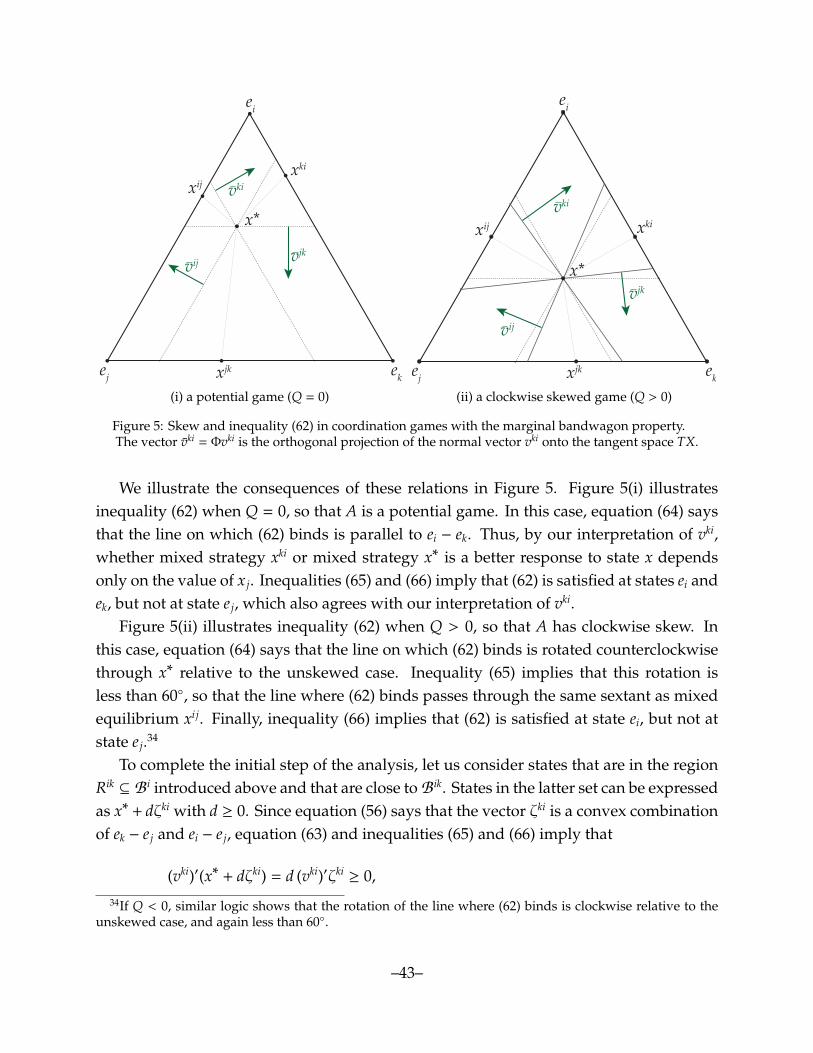
properties. We first consider the exit problem, which is used to assess the expected timeuntil the evolutionary process leaves the basin of attraction of a stable equilibrium, andto determine the likely exit path. Solving this problem for the class of games underconsideration, we show that the likely exit path proceeds along the boundary of thesimplex, escaping the basin of attraction through a boundary mixed equilibrium.

To evaluate stationary distribution asymptotics and stochastic stability, one must in-stead consider the transition problem, which is used to assess the probable time until atransition between a given pair of stable equilibria, and the most likely path that thistransition will follow. We solve the transition problem explicitly for simple three-strategycoordination games, and find that the nature of the problem’s solution depends in a basicway on whether the game in question is also a potential game. When this is so, theoptimal control problem is degenerate, in that there are open sets of states from whichthere are a continuum of minimal cost paths. Still, the optimal paths between equilibriaalways proceed directly along the relevant edge of the simplex. The control problem isnot degenerate for games without a potential function, which we call skewed games. Butunlike in the case of potential games, optimal paths between equilibria of skewed gamesneed not be direct; instead, they may proceed along an alternate edge of the simplex, turninto the interior, and pass through the interior equilibrium.

By combining solutions to the control problems with our earlier results, we are able tocharacterize the long run behavior of the evolutionary process in the small noise doublelimit. We use a parameterized class of examples to illustrate the effects of payoff-dependentmistake probabilities on equilibrium selection, and to contrast long-run behavior in thelogit and BRM models. In addition, in the class of potential games we consider, we fullydescribe the asymptotic behavior of the stationary distribution in the small noise doublelimit, showing that the rate of decay of the stationary distribution mass at each state equalsthe difference between the value of the potential function at that state and the maximumvalue of potential. In contrast to those in previous work on logit choice in potentialgames,7 the assumptions we impose on the transition law of the evolutionary processare asymptotic in nature, and so do not allow us to express the stationary distribution inclosed form. We instead build our analysis on large deviations estimates, and therebyobtain a clearer intuition about the form that the stationary distribution asymptotics take.

While the optimal control problems we solve have nonsmooth running costs, they aresimple in other respects. If L(x,u) represents the cost of choosing direction of motionu at state x, then L is piecewise linear in u regardless of the agents’ choice rule. Whenagents employ the logit choice rule, L is also piecewise linear in x. Taking advantage of

7See Blume (1993, 1997) and Sandholm (2010c, Sec. 11.5 and 12.2), as well as Section 7.6 below.

–5–

these properties, we use sufficient conditions for optimality due to Boltyanskii (1966) andPiccoli and Sussmann (2000) to construct candidate value functions, and to verify thatthey are indeed the value functions for our problems. These sufficient conditions requirethe value function to be continuous, to be continuously differentiable except on a finiteunion of manifolds of positive codimension, and to satisfy the Hamilton-Jacobi-Bellmanequation wherever the value function is smooth. In our case, for each fixed state x, thepiecewise linearity of L(x,u) in u means that only a small number of controls need tobe considered, while the piecewise linearity of L(x,u) in x makes it enough to check theHamilton-Jacobi-Bellman equation at a small number of well-chosen states.

These properties of the optimal control problem are not dependent on the class ofgames we consider, but only on the linearity of payoffs in the population state. Moreover,much of the structure of the problem is retained under alternatives to the logit choicerule. Thus as we explain in the final section of the paper, it should be possible to usethe approach developed here to study long run behavior in broader classes of games andunder other choice rules.

While work in stochastic evolutionary game theory typically focuses on stochasticstability and equilibrium selection, we feel that the dynamics of transitions betweenequilibria are themselves of inherent interest. Just as theories of disequilibrium learningoffer explanations of how and when equilibrium play may arise, models of transitiondynamics suggest how equilibrium is likely to break down. The importance of thisquestion has been recognized in macroeconomics, where techniques from large deviationstheory have been used to address this possibility in a variety of applications; see Choet al. (2002), Williams (2014), and the references therein. The present paper addressesthis question in an environment where the stochastic process arises endogenously as adescription of the aggregate behavior of a population of strategically interacting agents.

A number of earlier papers on stochastic evolution have considered small noise doublelimits. Binmore et al. (1995) and Binmore and Samuelson (1997) (see also Sandholm (2012))analyze models of imitation with mutations, focusing on two-strategy games; see Section8.1 for a discussion. Fudenberg and Imhof (2006, 2008) extend these analyses to themany-strategy case. The key insight of the latter papers is that under imitation withmutations, the stochastic evolutionary process is nearly always at vertices or on edgesof the simplex. Because of this, transitions between equilibria can be analyzed as one-dimensional problems using birth-death chain methods. In contrast, in the noisy bestresponse models studied here, the least costly transition between a pair of pure equilibriamay pass through the interior of the simplex.

Turning to noisy best response models, Kandori and Rob (1995, 1998) and Ellison (2000)

–6–

analyze stochastic evolution under the BRM rule in the small noise double limit. Blume(2003) and Sandholm (2010b) use birth-death chain techniques to study this limit in two-strategy games when mistake probabilities are payoff dependent. In the work closest tothe present one, Staudigl (2012) studies the small noise double limit when two populationsare matched to play 2x2 coordination games. The analysis uses optimal control methodsto evaluate the probabilities of transitions between equilibria. It takes advantage of thefact that each population’s state variable is scalar, and only affects the payoffs of membersof the opposing population; this causes the control problem to retain a one-dimensionalflavor absent from the general case.

The paper proceeds as follows. Section 2 introduces our class of stochastic evolutionaryprocesses. Section 3 reviews stochastic stability in the small noise limit. The followingthree sections study the small noise double limit. Section 4 provides definitions, Section5 presents the main technical results on the convergence of exit and transition costs, andSection 6 describes the consequences for escape from equilibrium, limiting stationarydistributions, and stochastic stability. Section 7 combines the foregoing analysis withoptimal control techniques to study long run behavior in a class of coordination gamesunder the logit choice rule. Section 8 offers concluding discussions. Many proofs andauxiliary results are presented in the Appendix, and a table listing all notation used in thepaper appears before the References.

2. The Model

2.1 Finite-population games

We consider games in which agents from a population of size N choose strategies fromthe common finite strategy set S. The population’s aggregate behavior is described by apopulation state x, an element of the simplex X = x ∈ Rn

+ :∑n

i=1 xi = 1, or more specifically,the grid X N = X ∩ 1

NZn = x ∈ X : Nx ∈ Zn

. The standard basis vector ei ∈ X ⊂ Rn

represents the pure population state at which all agents play strategy i. States that are notpure are called mixed population states.

We identify a finite-population game with its payoff function FN : X N→ Rn, where

FNi (x) ∈ R is the payoff to strategy i when the population state is x ∈ X N. Only the values

that the function FNi takes on the set X N

i = x ∈ X N : xi > 0 are meaningful, since at theremaining states in X N strategy i is unplayed.

Example 2.1. Suppose that N agents are matched to play a symmetric two-player normal

–7–

form game A ∈ Rn×n. If self-matching is not allowed, then payoffs take the form

(1) FNi (x) = 1

N−1 e′iA(Nx − ei) = (Ax)i + 1N−1 ((Ax)i − Aii). _

In a finite-population game, an agent who switches from strategy i to strategy j whenthe state is x changes the state to the adjacent state y = x + 1

N (e j − ei). Thus at any givenpopulation state, players playing different strategies face slightly different incentives. Toaccount for this, we use the clever payoff function FN

i→· : X Ni → R

n to denote the payoff

opportunities faced by i players at each state x ∈ X Ni . The jth component of the vector

FNi→·(x) is thus

(2) FNi→ j(x) = FN

j (x + 1N (e j − ei)).

Clever payoffs allow one to describe Nash equilibria of finite-population games in asimple way. The pure best response correspondence for strategy i ∈ S in finite-populationgame FN is denoted by bN

i : X Ni ⇒ S, and is defined by

(3) bNi (x) = argmax

j∈SFN

i→ j(x).

State x ∈ X N is a Nash equilibrium of FN if no agent can obtain a higher payoff by switchingstrategies: that is, if i ∈ bN

i (x) whenever xi > 0.

Example 2.2. The normal form game A ∈ Rn×n is a coordination game if Aii > A ji for alldistinct i, j ∈ S, so that if one’s match partner plays i, one is best off playing i oneself.If FN is the population game obtained by matching in A without self-matching, then theNash equilibria of FN are precisely the pure population states. Thus finite-populationmatching differs from continuous-population matching, under which the Nash equilibriaof the population game correspond to the pure and mixed symmetric Nash equilibria ofA.

To see that no mixed population state of FN can be Nash, suppose that x ∈ X Ni ∩ X N

j isa Nash equilibrium. Then

FNi (x) ≥ FN

j (x + 1N (e j − ei)) and FN

j (x) ≥ FNi (x + 1

N (ei − e j)),

which with (1) is equivalent to

(4) Ne′iAx − Aii ≥ Ne′jAx − A ji and Ne′jAx − A j j ≥ Ne′iAx − Ai j.

–8–

Summing these inequalities and rearranging yields (Aii−A ji)+(A j j−Ai j) ≤ 0, contradictingthat A is a coordination game. Furthermore, pure state ei is a Nash equilibrium if FN

i (x) ≥FN

j (x + 1N (e j − ei)) for j , i, which from (4) is true if and only if Aii > A ji, as assumed. _

It is convenient to assume that revising agents make decisions by considering cleverpayoffs, as it ensures that all agents are content if and only if the current state is a Nashequilibrium. The previous example shows that in a coordination game, such a state mustbe pure. While the use of clever payoffs simplifies the finite population dynamics—inparticular, by ensuring that in coordination games, only pure states are rest points—itdoes not affect our results on large population limits in an essential way.

2.2 Noisy best response protocols and unlikelihood functions

In our model of stochastic evolution, agents occasionally receive opportunities toswitch strategies. Upon receiving a revision opportunity, an agent selects a strategy byemploying a noisy best response protocol ση : Rn

→ int(X) with noise level η > 0, a functionthat maps vectors of payoffs to probabilities of choosing each strategy.

To justify its name, the protocol ση should recommend optimal strategies with highprobability when the noise level is small:

(P1) j < argmaxk∈S

πk ⇒ limη→0

σηj (π) = 0.

Condition (P1) implies that if there is a unique optimal strategy, then this strategy isassigned a probability that approaches one as the noise level vanishes. For simplicity,we also require that when there are multiple optimal strategies, each retains positiveprobability in the small noise limit:

(P2) j ∈ argmaxk∈S

πk ⇒ limη→0

σηj (π) > 0.

To analyze large deviations and stochastic stability, we must impose regularity con-ditions on the rates at which the probabilities of choosing suboptimal strategies vanishas the noise level η approaches zero. To do so, we introduce the unlikelihood functionΥ : Rn

→ Rn+, defined by

(5) Υ j(π) = − limη→0

η log σηj (π).

–9–

This definition can be expressed equivalently as

σηj (π) = exp(−η−1(Υ j(π) + o(1))

).

Either way, the unlikelihood Υ j(π) represents the rate of decay of the probability thatstrategy j is chosen as η approaches zero. Because they are defined using logarithmsof choice probabilities, the unlikelihoods of (conditionally) independent choices combineadditively. This fact plays a basic role in the analysis—see Section 3.2.8

We maintain the following assumptions throughout the paper:

The limit in (5) exists for all π ∈ Rn.(U1)

Υ is continuous.(U2)

Υ j(π) = 0 if and only if j ∈ argmaxk∈S πk.(U3)

Note that the “if” direction of condition (U3) is implied by condition (P2), and thatcondition (U1) and the “only if” direction of condition (U3) refine condition (P1).

We proceed with three examples that satisfy the conditions above.

Example 2.3. Logit choice. The logit choice protocol with noise level η, introduced to evolu-tionary game theory by Blume (1993), is defined by

(6) σηj (π) =exp(η−1π j)∑

k∈S exp(η−1πk).

It is well known that this protocol can be derived from an additive random utility modelwith extreme-value distributed shocks, or from a model of choice among mixed strategieswith control costs given by an entropy function.9 It is easy to verify that this protocolsatisfies conditions (U1)–(U3) with piecewise linear unlikelihood function

Υ j(π) = maxk∈S

πk − π j. _

Example 2.4. Random utility with averaged shocks. Consider an additive random utilitymodel in which the payoff vector π is perturbed by adding the sample average εm of ani.i.d. sequence ε`m`=1 of random vectors, where the n components of ε` are drawn from acontinuous distribution with unbounded convex support and whose moment generating

8Blume (2003) and Sandholm (2010b) place assumptions on the rates of decay of choice probabilities inthe context of two-strategy games. Unlikelihood functions for choice problems with many alternatives areintroduced by Dokumacı and Sandholm (2011); see Example 2.4 below.

9See Anderson et al. (1992) or Hofbauer and Sandholm (2002).

–10–

function exists. Writing η for 1m , we obtain the protocol

σηj (π) = P

(j ∈ argmax

k∈S(πk + εm

k ))

Dokumacı and Sandholm (2011) show that the limit (5) exists for each π ∈ Rn, andcharacterize the function Υ in terms of the Cramer transform of ε`. They also show that Υ j

is nonincreasing in π j, nondecreasing in πk for k , j, and convex (and hence continuous)in π. _

Example 2.5. Probit choice. Following Myatt and Wallace (2003), consider an additiverandom utility model in which the payoff vector π is perturbed by a multivariate normalrandom vector whose components are independent with common variance η. Since theaverage of independent normal random variables is normal, the probit choice model is aspecial case of Example 2.4. Dokumacı and Sandholm (2011) provide an explicit, piecewisequadratic expression for the unlikelihood function Υ. _

The only noisy best response protocol commonly considered in the literature thatdoes not satisfy our assumptions is the best response with mutations (BRM) protocol ofKandori et al. (1993), the focus of much of the literature to date. Under this protocol, anysuboptimal strategy has unlikelihood 1, and a unique optimal strategy has unlikelihood0, so condition (U2) must fail. For further discussion of the BRM protocol, see Remark7.10 and Example 7.12.

2.3 The stochastic evolutionary process

A population game FN and a revision protocol ση define a stochastic evolutionaryprocess. The process runs in discrete time, with each period taking 1

N units of clock time.During each period, a single agent is chosen at random from the population. This

agent updates his strategy by applying the noisy best response protocol ση. As discussedin Section 2.1, we assume that agents are clever, so that an i player evaluates payoffs usingthe clever payoff vector FN

i→·(x) defined in (2).This procedure described above generates a Markov chain XN,η = XN,η

k ∞

k=0 on the statespace X N. The index k denotes the number of revision opportunities that have occurredto date, and corresponds to k

N units of clock time. The transition probabilities PN,ηx,y for the

–11–

process XN,η are given by

(7) PN,ηx,y ≡ P

(XN,η

k+1 = y∣∣∣ XN,η

k = x)

=

xi σ

ηj (F

Ni→·(x)) if y = x + 1

N (e j − ei), j , i∑ni=1 xi σ

ηi (FN

i→·(x)) if y = x,

0 otherwise.

It is easy to verify that∑

y∈X N PN,ηx,y = 1 for all x ∈ X N.

A realization of the process XN,η over its first `N < ∞ periods is described by a paththrough X N of length `N, a sequence φN = φN

k `N

k=0 in which successive states either areidentical or are adjacent in X N. Since each period lasts 1

N time units, the duration of thispath in clock time is TN = `N/N.

Since revising agents are chosen at random and play each strategy in S with positiveprobability, the Markov chain XN,η is irreducible and aperiodic, and so admits a uniquestationary distribution, µN,η. It is well known that the stationary distribution is the limitingdistribution of the Markov chain, as well as its limiting empirical distribution along almostevery sample path.

3. The Small Noise Limit

We now consider the behavior of the stochastic process XN,η as the noise level η ap-proaches zero, proceeding from short run through very long run behavior. Over shortto medium time scales, XN,η is nearly a discrete best response process. We introduce thisbest response process and its recurrent classes in Section 3.1. Over longer periods, runs ofsuboptimal choices occasionally occur, leading to transitions between the recurrent classesof the best response process. We consider these in Sections 3.2 and 3.3. Finally, over verylong time spans, XN,η spends the vast majority of periods at the stochastically stable states,which we define in Section 3.4. Most of the ideas presented in this section can be foundin the evolutionary game literature, though not always in an explicit form.

3.1 The discrete best response dynamic and its recurrent classes

In the literature on stochastic evolution in games, the Markov chain XN,η is typicallyviewed as a perturbed version of some “unperturbed” process XN,0 based on exact bestresponses. To define the latter process as a Markov chain, one must specify the probabilitywhich which each best response is chosen when more than one exists. Here we take amore general approach, defining XN,0 not as a Markov chain, but by way of a difference

–12–

inclusion—in other words, using set-valued deterministic dynamics.Fix a population size N and a game FN. Suppose that during each discrete time period,

a single agent is chosen from the population, and that he selects a strategy that is optimalgiven the current population state and his current strategy. If the current state is x ∈ X N,then the set of increments in the state that are possible under this procedure is 1

N VN(x),where

(8) VN(x) = e j − ei : i ∈ s(x) and j ∈ bNi (x),

and where s(x) = i ∈ S : xi > 0 denotes the support of state x. The paths through X N thatcan arise under this procedure are the solutions to the difference inclusion

(DBR) xNk+1 − xN

k ∈1N

VN(xNk ).

We call (DBR) the discrete best response dynamic.We call the set KN

⊆ X N strongly invariant under (DBR) if no solution to (DBR) startingin KN ever leaves KN. A set that is minimal with respect to this property is called a recurrentclass of (DBR). We denote the collection of such recurrent classes by K N.10

Example 3.1. Let FN be defined by random matching in the normal form coordinationgame A as in Example 2.2, so that the Nash equilibria of FN are the pure states. Suppose inaddition that A has the marginal bandwagon property of Kandori and Rob (1998): Aii −Aik >

A ji − A jk for all i, j, k ∈ S with i < j, k. This property requires that when some agentswitches to strategy i from any other strategy k, current strategy i players benefit most. Aneasy calculation shows that in games with this property, i ∈ bN

i (x) implies that i ∈ bNk (x) for

all k ∈ s(x); this is a consequence of the fact that a strategy i player has one less opponentplaying strategy i than a strategy k , i player.

Now suppose that state x ∈ X N is not a Nash equilibrium. Then there are distinctstrategies i and j such that j ∈ s(x) ( j is in use) and i ∈ bN

j (x) (i is optimal for agents playingj), so that a step from x to y = x + 1

N (ei − e j) is allowed under (DBR). Since i ∈ bNj (x) is

equivalent to i ∈ bNi (x + 1

N (ei − e j)), the marginal bandwagon property (specifically, theclaim ending the previous paragraph) implies that i ∈ bN

k (y) for all k ∈ s(y). Repeatingthis argument shows that any path from y along which the number of strategy i playersincreases until pure state ei is reached is a solution to (DBR). We conclude that the recurrent

10One can represent the solutions and the recurrent classes of (DBR) using a suitably chosen Markovchain XN,∗. Define XN,∗ by supposing that during each period, a randomly chosen agent receives a revisionopportunity and switches to a best response, choosing each with equal probability (or, more generally, withany positive probability). Then a finite-length path is a solution to (DBR) if and only if it has positiveprobability under XN,∗, and the recurrent classes of (DBR) as defined above are the recurrent classes of XN,∗.

–13–

classes of (DBR) correspond to the pure states, K N = e1, . . . , en, as shown by Kandoriand Rob (1998).11 _

Example 3.2. Again let FN be defined by random matching in the normal form coordinationgame A. If x ∈ XN is not Nash, there is a strategy j in the support of x satisfying j < bN

j (x).Lemma A.1 in Appendix A.1 shows that in this case, there is a solution to (DBR) startingfrom x along which the number of j players decreases until j is unused.

Now suppose further that in game FN, switching to an unused strategy is never optimal:j ∈ bN

i (x) implies that x j > 0. In this case, applying Lemma A.1 inductively shows that fromevery state x ∈ XN, there is a solution to (DBR) that terminates at a pure state, implyingthat K N = e1, . . . , en. _

We conjecture that the set of recurrent classes of (DBR) is K N = e1, . . . , en for anycoordination game as defined in Example 2.2. Example 4.1 establishes a version of thisclaim for the large population limit.

3.2 Step costs and path costs

When the noise level η is small, the process XN,η will linger in recurrent classes, butwill occasionally transit between them. We now work toward describing the probabilitiesof these transitions in the small noise limit.

To begin, we define the cost of a step from x ∈ X N to y ∈ X N by

(9) cNx,y = − lim

η→0η log PN,η

x,y .

with the convention that −log 0 = +∞. Thus cNx,y is the exponential rate of decay of the

probability of a step from x to y as η approaches 0. Using definitions (5) and (7), we canrepresent step costs in terms of the game’s payoff function and the protocol’s unlikelihoodfunction:

(10) cNx,y =

Υ j(FN

i→·(x)) if y = x + 1N (e j − ei) and j , i,

mini∈s(x)

Υi(FNi→·(x)) if y = x, and

+∞ otherwise.

The important case in (10) is the first one, which says that the cost of a step in which ani player switches to strategy j is the unlikelihood of strategy j given i’s current payoff

11Unlike our model, the model of Kandori and Rob (1995, 1998) allows multiple revisions during eachperiod; see also footnote 18 below.

–14–

opportunities.12 By virtue of (10) and condition (U3), a step has cost zero if and only if itis feasible under the discrete best response dynamic:

(11) cNx,y = 0 ⇔ y − x ∈ VN(x).

The cost of path φN = φNk `N

k=0 of length `N < ∞ is the sum of the costs of its steps:

(12) cN(φN) =

`N−1∑

k=0

cNφN

k ,φNk+1.

Definitions (7) and (10) imply that the cost of a path is the rate at which the probability offollowing this path decays as the noise level vanishes: for fixed N, we have

P(XN,η

k = φNk , k = 0, . . . , `N

∣∣∣ XN,η0 = φN

0

)=

`N−1∏

k=0

PN,ηφN

k ,φNk+1≈ exp(−η−1cN(φN)).

where ≈ refers to the order of magnitude in η as η approaches zero. By statement (11),path φN has cost zero if and only if it is a solution to (DBR).

3.3 Exit costs and transition costs

We now consider escape from and transitions between recurrent classes. Let KN∈ K N

be a recurrent class of (DBR), and let ΞN⊂ X N be a set of states. We define ΦN(KN,ΞN) to

be the set of finite-length paths through X N with initial state in KN and terminal state inΞN, so that

(13) CN(KN,ΞN) = mincN(φN) : φN∈ ΦN(KN,ΞN)

is the minimal cost of a path from KN to ΞN.If ΞN is a union of recurrent classes from K N, we define the weak basin of attraction of

ΞN, denoted W N(ΞN), to be the set of states in X N from which there is a zero-cost paththat terminates at a state in ΞN. Notice that by definition,

CN(KN,ΞN) = CN(KN,W N(ΞN)).

We also define ΩN(KN,W N(ΞN)) ⊆ W N(ΞN) to be the set of terminal states of cost mini-12The second case of (10) indicates that at a state where no agent is playing a best response, staying still

is costly. Since staying still does not facilitate transitions between recurrent classes, this possibility is notrealized on minimum cost paths, but we must account for it carefully in what follows—see Section 4.3.2.

–15–

mizing paths from KN to W N(ΞN) that do not hit W N(ΞN) until their final step.Two specifications of the target set ΞN are of particular interest. First, let

(14) KN =⋃

LN∈K NrKN

LN

be the union of the recurrent classes other than KN. We call CN(KN, KN) the cost of exitfrom KN.13 Proposition 3.3 provides an interpretation of this quantity. Here τN,η(ΞN) =

mink : XN,ηk ∈ ΞN

denotes the time at which the process XN,η first hits ΞN.

Proposition 3.3. Suppose that XN,η0 = xN

∈ KN for all η. Then

(i) limη→0

η logEτN,η(KN) = limη→0

η logEτN,η(W N(KN)) = CN(KN, KN);

(ii) limη→0

η logP(XN,ητN,η(W N(KN))

= y) = 0 if and only if y ∈ ΩN(KN,W N(KN)).

Part (i) of the proposition shows that when η is small, the expected time required for theprocess to escape from KN to another recurrent class is of order exp(η−1CN(KN, KN)). Part (ii)shows that the the states in W N(KN) most likely to be reached first are the terminal statesof cost minimizing paths from KN to W N(KN). Both parts follow by standard argumentsfrom Proposition 4.2 of Catoni (1999), which provides a discrete-state analogue of theFreidlin and Wentzell (1998) theory.

Proposition 3.3 concerns behavior within the strong basin of attraction of KN, the set ofstates S N(KN) = X N rW N(KN) ⊆ W N(KN) from which there is no zero-cost path to anyother recurrent class. But to understand the global behavior of the process, we must alsoconsider transitions from KN to each other individual recurrent class in K N.

When LN∈ K N, we call CN(KN,LN) the cost of a transition from KN to LN. Intuitively,

CN(KN,LN) describes the likely order of magnitude of the time until LN is reached. Butwhile the analogue of Proposition 3.3(ii) on the likely points of entry into W N(LN) is true,the analogue of Proposition 3.3(i) on the expected hitting time of LN is false in general,since this expectation may be driven by a low probability of becoming stuck in some thirdrecurrent class.14

3.4 Stationary distribution asymptotics and stochastic stability

The transition costs CN(KN,LN) are the basic ingredient in Freidlin and Wentzell’s(1998) graph-theoretic characterization of limiting stationary distributions and stochastic

13Thus the cost of exit from KN corresponds to the radius of KN as defined by Ellison (2000).14This is the reason for the correction term appearing in Proposition 4.2 of Catoni (1999). See Freidlin and

Wentzell (1998, p. 197–198) for a clear discussion of this point.

–16–

stability. According to this characterization, there is a function ∆rN : X N→ R+, defined in

terms of the aggregate costs of certain graphs on X N, such that

(15) − limη→0

η logµN,η(x) = ∆rN(x) for all x ∈ X N.

Thus ∆rN(x) describes the exponential rate of decay of the stationary distribution weighton x as η approaches zero.

We call state x ∈ X N stochastically stable in the small noise limit if as η approaches 0, itsstationary distribution weight µN,η(x) does not vanish at an exponential rate.15 By virtue of(15), state x is stochastically stable in this sense if and only if ∆rN(x) = 0. Since these ideasare well known in evolutionary game theory,16 we postpone the detailed presentationuntil Section 6.2.

4. The Small Noise Double Limit

The exit costs and transition costs introduced in Section 3.3, defined in terms of min-imum cost paths between sets of states in X N, describe the transitions of the process XN,η

between recurrent classes when the noise level η is small. When step costs depend onpayoffs, finding these minimum cost paths is a challenging computational problem.

We contend with this difficulty by taking a second limit: after taking the noise levelη to 0, we take the population size N to infinity, thus evaluating behavior in the smallnoise limit when the population size is large. In the remainder of this paper, we showhow one can evaluate this double limit by approximating the discrete constructions fromthe previous section by continuous ones. In particular, taking the second limit here turnsthe path cost minimization problem (13) into an optimal control problem. Although thisproblem is nonsmooth and multidimensional, it is nevertheless simple enough to admitanalytical solutions in interesting cases.

4.1 Limits of finite-population games

To consider large population limits, we must specify a notion of convergence forsequences FN

∞

N=N0of finite-population games. If such a sequence converges, its limit is

a (continuous) population game, F : X → Rn, which we take to be a continuous function

15Explicitly, this means that for all δ > 0 there is an η0 > 0 such that for all η < η0, µN,η(x) > exp(−ηδ). Thisdefinition of stochastic stability is slightly less demanding than the one appearing in Kandori et al. (1993)and Young (1993); Sandholm (2010c, Sec. 12.A.5) explains this distinction in detail.

16See Young (1993, 1998), Kandori and Rob (1995), and Sandholm (2010c, Section 12.A).

–17–

from the compact set X to R. The pure and mixed best response correspondences for thepopulation game F are denoted by b : X⇒ S and B : X⇒ X, and are defined by

b(x) = argmaxi∈S

Fi(x) and B(x) = y ∈ X : supp(y) ⊆ b(x) = argmaxy∈X

y′F(x).

State x is a Nash equilibrium of F if i ∈ b(x) whenever xi > 0, or, equivalently, if x ∈ B(x).The notion of convergence we employ for the sequence FN

∞

N=N0is uniform conver-

gence, which asks that

(16) limN→∞

maxx∈X N

∣∣∣FN(x) − F(x)∣∣∣ = 0,

where | · | denotes the `1 norm on Rn. It is easy to verify that under this notion of con-vergence, the Nash equilibrium correspondences for finite-population games are “upperhemicontinuous at infinity”: if the sequence of games FN

converges to F, the sequenceof states xN

converges to x, and if each xN is a Nash equilibrium of the corresponding FN,then x is a Nash equilibrium of F.

When agents are matched to play a symmetric two-player normal form game A ∈Rn×n (Example 2.1), it is easy to verify that uniform convergence obtains with the limitgame given by F(x) = Ax. It is also easy to verify that if a sequence of populationgames converges uniformly, then the clever payoff functions associated with that gameall converge uniformly to the same limit.

4.2 The complete best response dynamic and limiting recurrent classes

The solutions of the discrete best response dynamic (DBR) are the paths through X N

that can be traversed at zero cost. To define the analogous dynamic for the large populationlimit, let S(x) = y ∈ X : s(y) ⊆ s(x) be the set of states whose supports are contained in thesupport of x. Then the complete best response dynamic is the differential inclusion

x ∈ B(x) − S(x)(CBR)

= β − α : β ∈ B(x), α ∈ S(x)

= conv(e j − ei | i ∈ s(x), j ∈ b(x)).

Comparing the final expression above to definition (8), we see that (CBR) is the continuous-time analogue of the discrete best response dynamic (DBR), obtained by taking the largeN limit of (DBR) and convexifying the result. We will soon see that solutions to (CBR)correspond to zero-cost continuous paths under our limiting path cost function.

–18–

e1

e2 e3

x B(x)–xB(x)–S(x)

Figure 1: The dynamics (BR) and (CBR) and in a three-strategy game from a state x with b(x) = 1.

For intuition, we contrast (CBR) with the standard model of best response strategyrevision in a large population—the best response dynamic of Gilboa and Matsui (1991):

(BR) x ∈ B(x) − x.

To obtain (BR) as the limit of finite-population dynamics, one assumes that in each discretetime period, an agent is chosen at random from the population and then updates to a bestresponse. As the population size grows large, the law of large numbers ensures that therates at which the various strategies are abandoned are proportional to the prevalences ofthe strategies in the population, generating the −x outflow term in (BR).17 Thus at stateswhere the best response is unique, (BR) specifies a single vector of motion, as shown inFigure 1 at a state at which the unique best response is strategy 1. Under (DBR), thereis no presumption that revision opportunities are assigned at random. Thus, in the largepopulation limit (CBR), the strategies present in the population can be abandoned at anyrelative rates, leading to the −S(x) outflow term in (CBR). In Figure 1, the set of vectors ofmotion under (CBR) is the convex hull of the vectors e1 − e2, e1 − e3, and 0.18

In the classes of coordination games considered in Examples 3.1 and 3.2, the set K N ofrecurrent classes of the discrete best response dynamic (DBR) is equal to K = e1, . . . , en

17See Roth and Sandholm (2013) for a formal limit result.18Kandori and Rob (1995, 1998) consider a discrete-time best response dynamic in which any subset of

the players may revise during any period; for instance, the entire population may switch to a current bestresponse simultaneously. Figure 1 of Kandori and Rob (1995), used to illustrate this discrete-time dynamic,resembles Figure 1 above, but the processes these figures represent are different.

–19–

for every population size. We now show that in any coordination game, we can view thisK as the set of “recurrent classes” of the complete best response dynamic (CBR).

Example 4.1. Consider the continuous population game F(x) = Ax generated by a coordi-nation game A (Example 2.2). Since each pure state ei is a strict equilibrium, the uniquesolution to (CBR) starting at ei is the stationary trajectory. At any state ξ in the best re-sponse region B i = x ∈ X : (Ax)i ≥ (Ax) j for all j ∈ S, the vector ei − ξ, which pointsdirectly from ξ to ei, is a feasible direction of motion under the best response dynamic(BR). Since B i is convex and contains ei, motion can continue toward ei indefinitely: thetrajectory xtt≥0, defined by xt = e−tξ+ (1−e−t)ei, is a solution to (BR), and hence a solutionto (CBR). Thus for any coordination game F(x) = Ax, starting from any initial conditionξ ∈ X, there is solution to (CBR) that converges to a pure, and hence stationary, populationstate. _

More generally, the exact positions of the recurrent classes of the discrete best responsedynamic (DBR) will vary with the population size. To allow for this, we assume that thereis a set K = K1, . . . ,Kκ of disjoint closed subsets of X called limiting recurrent classes. Tojustify this name, we require that for some constant d > 0 and all large enough populationsizes N, the dynamic (DBR) has κ recurrent classes, K N = KN

1 , . . . ,KNκ , and that

(17) dist(KNi ,Ki) ≤

dN

for all i ∈ 1, . . . , κ,

where dist(KNi ,Ki) denotes the `1-Hausdorff distance between KN

i and Ki19

4.3 Costs of continuous paths

To evaluate stochastic stability in the small noise double limit, we need to determinethe costs CN(KN,ΞN), defined by the discrete cost minimization problems (13) on X N, forlarge values of N. To prepare for our continuous approximation of these problems, wenow introduce a definition of costs for continuous paths through the simplex X.

4.3.1 Discrete paths, derivatives, and interpolations

Let φN = φNk `N

k=0 be a path for the N-agent process. Since each period of this processtakes 1

N units of clock time, we define

(18) φNk = N(φN

k+1 − φNk )

19That is, dist(KNi ,Ki) = max

maxx∈KN

i

miny∈Ki|x − y|,max

y∈Kiminx∈KN

i

|x − y|, where | · | is the `1 norm on Rn.

–20–

to be the discrete right derivative of path φN at time k. Let ıN(k) ∈ S and N(k) ∈ Sdenote the pre- and post-revision strategies of the agent who revises in period k. ThenφN

k+1 = φNk + 1

N (e N(k) − eıN(k)), and hence

(19) φNk = e N(k) − eıN(k).

Note that if ıN(k) = N(k), so that the revising agent does not switch strategies, then φNk = 0.

Each discrete path φNk `N

k=0 induces a continuous path φ(N)t t∈[0,`N/N] via piecewise affine

interpolation:

(20) φ(N)t = φN

bNtc + (Nt − bNtc)(φNbNtc+1 − φ

NbNtc).

This definition too accounts for each period in the N-agent process lasting 1N units of clock

time. Evidently, the derivative φ(N) of this process agrees with the discrete derivative φN

defined in (18), in the sense that

(21) φ(N)t = φN

bNtc whenever Nt < Z.

Speed of motion along a continuous path φtt∈[0,T] is measured most naturally byevaluating the `1 norm |φt| =

∑i∈S |(φt)i| of φt ∈ TX ≡ z ∈ Rn :

∑i∈S zi = 0, as this norm

makes it easy to separate the contributions of strategies that are gaining players from thoseof strategies that are losing players. If for z ∈ Rn we define [z]+ ∈ Rn

+ and [z]− ∈ Rn+ by

([z]+)i = [zi]+ and ([z]−)i = [zi]−, then by virtue of equations (19) and (21), any interpolatedpath φ(N) satisfies the following bound on its speed:

(22)∣∣∣[φ(N)

t ]+

∣∣∣ ≡ ∣∣∣[φ(N)t ]−

∣∣∣ ≤ 1, and thus∣∣∣φ(N)

t

∣∣∣ ≤ 2.

4.3.2 Costs of continuous paths

To work toward our definition of the cost of a continuous path, we now express thepath cost function (12) in a more suggestive form. Let 〈·, ·〉 denote the standard innerproduct on Rn, and let φN = φN

k `N

k=0 be a discrete path. If N(k) , ıN(k), then definitions(10) and (18) imply that the cost of step k is

(23) cNφN

k ,φNk+1

= Υ N(k)(FNıN(k)→·(φ

Nk )) = 〈Υ(FN

ıN(k)→·(φNk )), [φN

k ]+〉.

If N(k) = ıN(k), so that the revising agent does not switch strategies, then φNk equals

0; thus the rightmost expression of (23) evaluates to 0 for such null steps. This disagrees

–21–

with the second case of (10) when there is no best response to φNk is in its support. Since

this discrepancy only arises when a path lingers at some such state, it is inconsequentialwhen determining the minimal cost of a path between subsets of X N, as there is always aleast cost path that does not linger at all.

Summing up the step costs, the cost (12) of a discrete path φN without null steps canbe expressed as

(24) cN(φN) =

`N−1∑

k=0

cNφN

k ,φNk+1

=

`N−1∑

k=0

〈Υ(FNıN(k)→·(φ

Nk )), [φN

k ]+〉.

Now let φ : [0,T]→ X be absolutely continuous and non-pausing, meaning that |φt| , 0 foralmost all t ∈ [0,T]. Since FN

i→· ≈ F for large N, the form of the path costs in (24) suggeststhat the cost of φ should be defined as

(25) c(φ) =

∫ T

0〈Υ(F(φt)), [φt]+〉dt.

This derivation is informal; the formal justification of definition (25) is provided by theapproximation results to follow.

While the discrete path cost function (24) only concerns paths with discrete derivativesof the basic form φN

k = e N(k) − eıN(k), definition (25) allows any absolutely continuous pathwith derivatives φt in Z = conv(e j − ei : i, j ∈ S), or indeed in the tangent space TX. Thisextension combines two new ingredients. First, allowing φt to be the weighted average ofa number of vectors e j − ei makes it possible to approximate the cost of a continuous pathby the costs of rapidly oscillating discrete paths, a point we discuss further in Section 5.3.Second, by virtue of the linear homogeneity of the integrand of (25) in φt, the cost of acontinuous path is independent of the speed at which it is traversed.

Finally, we observe that a non-pausing absolutely continuous path φ has zero costunder (25) if and only if it is a solution of the complete best response dynamic (CBR).

5. The Convergence Theorem

In Section 3.3, we defined the minimal cost CN(KN,ΞN) of a discrete path from recurrentclass KN

∈ K N to set ΞN⊂ X N. We now consider a sequence of such problems, where the

recurrent classes KN converge to the limiting recurrent class K ∈ K as in condition (17),

–22–

and where the target sets ΞN⊂ X N converge to a closed set Ξ ⊂ X in the same sense:

(26) dist(ΞN,Ξ) ≤dN

for some d > 0 and all N large enough.Let Φ(K,Ξ) be the set of absolutely continuous paths of arbitrary duration through X

from K to Ξ, and define

(27) C(K,Ξ) = minc(φ) : φ ∈ Φ(K,Ξ)

to be the minimal cost of a continuous path from K to Ξ. Our aim in this section is to showthat the normalized optimal values of the discrete problems converge to the optimal valueof the continuous problem:

(28) limN→∞

1N

CN(KN,ΞN) = C(K,Ξ).

This conclusion will justify the definition (25) of the cost of a non-pausing absolutelycontinuous path, and will provide the tool needed to evaluate exit times, stationarydistribution asymptotics, and stochastic stability in the large population double limit.

5.1 Assumptions

We prove our results under two assumptions about the minimum cost path problems(13) and (27). To state the first assumption, which is needed to obtain the lower bound in(28), we recall that the duration TN = `N/N of the discrete path φN

k `N

k=0 is the number ofunits of clock time it entails.

Assumption 1. There exists a constant T < ∞ such that for all KN∈ K N, ΞN

⊂ X N, and N,there is a path of duration at most T that achieves the minimum in (13).

Since state space X N is finite, cost-minimizing paths between subsets of ΞN can alwaysbe assumed to have finite length. Assumption 1 imposes a uniform bound on the amountof clock time that these optimal paths require. It thus requires that cost-minimizing pathsnot become extremely convoluted as the population size grows large, as might be possibleif despite the uniform convergence of payoff functions in (16), the step costs cN

x,y definedin (10) became highly irregular functions of the current population state.

To introduce our second assumption, which is needed to obtain the upper boundin (28), we need some additional definitions. Let φ : [0,T] → X be a continuous path.

–23–

We call φ monotone if we can express the strategy set S as the disjoint union S+ ∪ S−,with φ j nondecreasing for j ∈ S+ and φi nonincreasing for i ∈ S−. If M is a positiveinteger, we say that φ is M-piecewise monotone if its domain [0,T] can be partitioned intoM subintervals such that φ is monotone on each; if this is true for some M, we say thatφ is piecewise monotone. Monotonicity and piecewise monotonicity for discrete paths aredefined analogously.

Motivated by bound (22), we say that piecewise monotone path φ moves at full speed if

(29)∣∣∣[φt]+

∣∣∣ ≡ ∣∣∣[φt]−∣∣∣ = 1, and thus

∣∣∣φt

∣∣∣ = 2, for almost all t ∈ [0,T].

By the linear homogeneity of the integrand of cost function (25), there is no loss if theminimum in (27) is taken over paths in Φ(K,Ξ) that move at full speed.

Assumption 2. There exist constants T < ∞ and M < ∞ such that for all K ∈ K andΞ ∈ K ∪

x

x∈X, there is an M-piecewise monotone, full speed path of duration at most Tthat achieves the minimum in (27).

Since the state space X is compact and the integrand of the cost function is (25) contin-uous, and since we may work with the compact, convex set of controls Z, it is reasonableto expect the minimum in (27) to be achieved by some finite-duration path. Piecewisemonotonicity is a mild regularity condition on the form of the minimizer. In practice,one applies the results developed below by explicitly solving control problem (27); in sodoing, one verifies Assumption 2 directly.

In order to appeal to Assumption 2, we assume in what follows that the target set Ξ iseither a limiting recurrent class or a singleton.20

5.2 The lower bound

To establish the convergence claim in (28), we must show that C(K,Ξ) provides both alower and an upper bound on the limiting behavior of 1

N CN(KN,ΞN).The key to obtaining the lower bound is to show that if the normalized costs 1

N cN(φN)of a sequence of discrete paths of bounded durations converge, then the costs c(φ(N)) ofthe corresponding linear interpolations converge to the same limit. This is the content ofthe following proposition. Its proof, which is based on continuity arguments, is presentedin Appendix A.2.

20For the results to follow that only concern recurrent classes, it is enough in Assumption 2 to considertarget sets in K . Singleton target sets are needed in Theorem 6.3 to derive the asymptotics of the stationarydistribution on the entire state space, rather than just its asymptotics on the recurrent classes.

–24–

Proposition 5.1. Let φN∞

N=N0be a sequence of paths with durations at most T and whose costs

satisfy limN→∞

1N cN(φN) = C∗. Then the corresponding sequence φ(N)

∞

N=N0of linear interpolations

satisfies limN→∞

c(φ(N)) = C∗.

Now consider a sequence (or, if necessary, a subsequence) of optimal discrete pathsφN∈ ΦN(KN,ΞN) for problem (13) with durations TN

≤ T (cf. Assumption 1) and whosecosts converge to C∗. By Proposition 5.1, the costs of their linear interpolations φ(N)

∈

Φ(KN,ΞN) also converge to C∗. We can extend these to paths in Φ(K,Ξ) by adding subpathslinking K to φ(N)

0 ∈ KN and φ(N)TN ∈ LN to L. Conditions (17) and (26) imply that this can

be done at negligible cost. This argument yields the following result, whose proof ispresented in Appendix A.3.

Proposition 5.2. lim infN→∞

1N CN(KN,ΞN) ≥ C(K,Ξ).

5.3 The upper bound

The key to obtaining the upper bound is to show that given a continuous path φ withcost c(φ), we can find a sequence of discrete paths φN

whose normalized costs approachc(φ). The natural approach to this problem is to define each φN as a suitable discreteapproximation of φ, and then to use continuity arguments to establish the convergence ofnormalized costs. But unlike the argument behind Proposition 5.1, the cost convergenceargument here is not straightforward. The earlier argument took advantage of the factthat every discrete path induces a continuous path via linear interpolation. Here, thediscrete approximation of the continuous path must be constructed explicitly.

Moreover, there are limits to what a discrete approximation can achieve. As definitions(24) and (25) state, a path’s cost depends on its derivatives at each point of time; thesederivatives specify the sequence of revisions that occur over the course of the path.However, one cannot always construct discrete approximations φN whose derivativesapproximate those of the continuous path φ.

As an illustration, consider Figure 2(i), which presents a continuous path φ throughX from vertex e1 to the barycenter ( 1

3 ,13 ,

13 ). As this path is followed, the state moves in

direction 12 (e2 + e3) − e1: the mass playing strategy 1 falls over time, while the masses

playing strategies 2 and 3 rise at equal rates. But discrete paths through X N are unableto move in this direction. At best, they can alternate between increments 1

N (e2 − e1) (i.e.,switches by a single agent from 1 to 2) and 1

N (e3 − e1). The states in the resulting discretepaths are all close to states in φ. But the alternation of increments needed to stay close toφ prevents the derivatives of the discrete paths from converging as N grows large.

–25–

(i) A continuous path through X (ii) A discrete path through X N (N = 30)

Figure 2: Discrete approximation of continuous paths.

Despite this difficulty, it is possible to construct discrete approximations φN whosecosts approach those of the continuous path φ, provided that φ is piecewise monotone.21

To begin, Proposition 5.3 shows that if φ is monotone and moves at full speed, then wecan find discrete paths φN that are also monotone and that closely approximate φ, in thatφN is within 2n

N of φ in the uniform norm.

Proposition 5.3. Suppose φ = φtt∈[0,T] is monotone and moves at full speed. If N ≥ 1T , there is

an sN∈ [0, 1

N ) and a feasible monotone path φN = φNk `N

k=0, `N =⌊N(T − sN)

⌋, satisfying

(30) max0≤k≤`N

∣∣∣∣φNk − φsN+ k

N

∣∣∣∣ ≤ 2nN.

A constructive proof of this proposition is presented in Appendix A.4.Next, Proposition 5.4 shows that the normalized costs of the discrete paths so con-

structed converge to the cost of the original path φ.

Proposition 5.4. Suppose that the path φtt∈[0,T] is monotone and moves at full speed, and that thepaths φN

k `N

k=0∞

N=N0are monotone and approximate φ in the sense of (30). Then lim

N→∞1N cN(φN) = c(φ).

The proof of Proposition 5.4 is presented in Appendix A.5, but we explain the logic ofthe proof here. By equation (24) and definition (18) of φN, we can express the normalized

21As an aside, we note that the continuous and discrete paths in Figure 2 are both monotone with S+ = 2, 3and S− = 1.

–26–

cost of path φN as

(31)1N

cN(φN) =

`N−1∑

k=0

〈Υ(FNıN(k)→·(φ

Nk )), [φN

k+1 − φNk ]+〉.

Because path φN is monotone, the second term in the inner product telescopes:

(32) [φNb − φ

Na ]+ =

b−1∑k=a

[φNk+1 − φ

Nk ]+

This property allows us to approximate (31) by a sum with only O(√

N) summands,each of which corresponds to O(

√N) terms in the original expression. This sum can be

approximated in turn by replacing values of φN with values of φ. Doing so yields aRiemann-Stieltjes sum (cf. (92)) whose integrator φ is monotone. Since there are O(

√N)

rather than O(N) summands, the O( 1N ) bound in (30) ensures that replacingφN withφ leads

to an approximation of 1N cN(φN) that is asymptotically correct.22 But since the number of

summands still grows without bound in N, the Riemann-Stieltjes sums converge as Ngrows large; their limit is the integral that defines c(φ).

By Assumption 2, there is a full speed, piecewise monotone optimal path φ ∈ Φ(K,Ξ)for problem (27). By Propositions 5.3 and 5.4, there are monotone discrete approximationsof each monotone segment of φ with total cost close to c(φ). To construct a path φN

∈

Φ(KN,ΞN), we patch together these monotone discrete approximations, and also addsegments from KN to φ0 ∈ K and from φT ∈ Ξ to ΞN. As before, conditions (17) and (26)ensure that this can be done at negligible cost. This argument yields the following upperbound, whose proof is presented in Appendix A.6.

Proposition 5.5. lim supN→∞

1N CN(KN,ΞN) ≤ C(K,Ξ).

Together, Propositions 5.2 and 5.5 establish the convergence of minimal path costs.

Theorem 5.6 (Convergence theorem). limN→∞

1N CN(KN,ΞN) = C(K,Ξ).

6. Consequences for Long Run Behavior

We now use the convergence theorem to characterize exit times, stationary distributionasymptotics, and stochastic stability in the small noise double limit. These characteriza-

22One can make an equivalent point in terms of derivatives: while φN does not converge to φ, the localaverages of φN over time intervals of length O(

√N) converge to the corresponding local averages of φ.

Compare Figure 2.

–27–

tions are stated in terms of solutions to the continuous control problems (27). As theseproblems are tractable in certain interesting cases, the results here allow one to obtainexplicit descriptions of the long run behavior of the stochastic evolutionary processes.

6.1 Expected exit times and exit locations

Given a recurrent class KN∈ K N, equation (14) defined KN as the union of the recurrent

classes in K N other than KN. Thus if the process XN,η starts in KN, then EτN,η(KN) is theexpected time until it reaches another recurrent class.

To characterize this expected waiting time, we let K be the limiting recurrent classcorresponding to KN (cf. equation (17)), and define

K =⋃

L∈K rKL

to be the union of the limiting recurrent classes other than K. Combining Proposition 3.3(i)and Theorem 5.6 immediately yields the following result.

Corollary 6.1. Let XN,η0 = xN

∈ KN for all η > 0 and N ≥ N0. Then

limN→∞

limη→0

η

NlogEτN,η(KN) = C(K, K).

In words, Corollary 6.1 says that when N is sufficiently large, the exponential growth rateof the expected waiting time EτN,η(KN) as η−1 vanishes is approximately N C(K, K). Thisquantity can be evaluated explicitly by solving control problem (27).

Turning to exit locations, Proposition 3.3(ii) showed that in the small noise limit, theexit point of XN,η from the strong basin of attraction S N(KN) = X NrW N(KN) is very likely tobe the terminal state of a minimum cost path from KN toW N(KN). Although the statementsof the main results in Section 5 focus on costs, their proofs establish that optimal discretepaths can be approximated arbitrarily well by nearly optimal continuous paths, and viceversa. It follows that the likely exit points of XN,η from S N(KN) can be approximated bythe terminal points of the optimal solutions of the appropriate control problems (27).

6.2 Stationary distribution asymptotics and stochastic stability

6.2.1 The small noise limit

To state our results on stationary distribution asymptotics and stochastic stability inthe small noise double limit, we first review the well-known results for the small noise

–28–

limit alluded to in Section 3.4. The analysis, which follows Freidlin and Wentzell (1998),is cast in terms of graphs on the set of recurrent classes K N.

A tree on K N with root KN, sometimes called a KN-tree, is a directed graph on K N

with no outgoing edges from KN, exactly one outgoing edge from each LN , KN, and aunique path though K N from each LN , KN to KN. Denote a typical KN-tree by τKN , andlet TKN denote the set of KN-trees. The cost of tree τKN on K N is the sum of the costs of thetransitions over its edges:

(33) CN(τKN ) =∑

(LN ,LN)∈τKN

CN(LN, LN).

Let RN : K N→ R+ assign each recurrent class KN

∈ K N the minimal cost of a KN-tree:

RN(KN) = minτKN∈TKN

CN(τKN ).

Then define the function rN : X N→ R+ by

(34) rN(x) = minKN∈K N

(RN(KN) + CN(KN, x)

).

If x is in recurrent class KN, then rN(x) = RN(KN). Otherwise, rN(x) is the sum of the cost ofsome KN-tree and the cost of a path from KN to x.23 Finally, let ∆rN : K N

→ R be a versionof rN whose values have been shifted to have minimum 0:

∆rN(x) = rN(x) −miny∈X N

rN(y).

Proposition 6.2 shows that the function ∆rN describes the exponential rates of decayof the the stationary distribution weights µN,η(x) in the small noise limit. It is an easyconsequence of Proposition 4.1 of Catoni (1999).

Proposition 6.2. The stationary distributions µN,η satisfy

(15) − limη→0

η logµN,η(x) = ∆rN(x) for all x ∈ X N.

6.2.2 The small noise double limit

To describe the asymptotics of the stationary distribution in the small noise doublelimit, we repeat the construction above using the set of limit recurrent classes K and the

23State x need not be in the weak basin of the recurrent class that yields the minimum in (34).

–29–

limit costs C. Denote a typical K-tree on the set of limiting recurrent classes K by τK, andlet TK denote the set of K-trees. Define the cost of tree τK by

C(τK) =∑

(L,L)∈τK

C(L, L).

Then define the functions R : K → R+, r : X→ R+, and ∆r : X→ R by

R(K) = minτK∈TK

C(τK), r(x) = minK∈K

(R(K) + C(K, x)) , and ∆r(x) = r(x) −miny∈X

r(y).

Theorem 6.3 describes the asymptotics of the stationary distributions µN,η in the smallnoise double limit.

Theorem 6.3. The stationary distributions µN,η satisfy

limN→∞

limη→0

maxx∈X N

∣∣∣− ηN logµN,η(x) − ∆r(x)

∣∣∣ = 0.

In words, the theorem says that when N is sufficiently large, the exponential rate of decayof µN,η(x) as η−1 approaches infinity is approximately N∆r(x).

A weaker version of Theorem 6.3, one that did not require uniformity of the largeN limit in x, would follow directly from Theorem 5.6 and Proposition 6.2.24 In order toprove Theorem 6.3 as stated, we need to show that the limit in Theorem 5.6 is uniformover all choices of the target set Ξ ∈ K ∪

x

x∈X (cf. Assumption 2). We accomplishthis in Appendix A.7 by bounding the rate of convergence in the results from Section 5independently of the specific paths and target sets under consideration. This uniform con-vergence in these earlier results directly yields the uniform asymptotics for the stationarydistributions.

In view of Theorem 6.3, we call state x ∈ X stochastically stable in the small noise doublelimit if for any open set O ⊂ X containing x, probability mass µN,η(O) does not vanishat an exponential rate in η once N is large enough.25 Theorem 6.3 implies that state x isstochastically stable in the small noise double limit if and only if ∆r(x) = 0.26

24In fact, since the number of recurrent classes is finite, a version of the theorem that focused only onthese would also follow directly from Theorem 5.6.

25Logically: ∀ δ > 0 ∀O ∈ O(X, x) ∃N0 ∈N ∀N > N0 ∃ η0 > 0 ∀ η < η0 µN,η(O) > exp(−ηδ), where O(X, x)denotes the set of open subsets of X containing x.

26This characterization remains true under a more demanding definition of stochastic stability, requiringthat for every δ > 0, there exist an O ∈ O(X, x) such that (leaving the quantifiers on N and η in place)µN,η(y) > exp(−ηδ) for every y ∈ O ∩ X N.

–30–

7. An Analysis of the Logit Model

To move from the results in the previous section to analyses of specific examples,one needs to solve instances of the path cost minimization problem (27). In this section,we show how to solve such problems using optimal control techniques, and combinethese solutions with the results below to describe long run play in particular examples.Our focus is on evolution under the logit choice rule (Example 2.3), in three-strategycoordination games (Example 2.2) that satisfy the marginal bandwagon property (Example3.1) and that have an interior equilibrium. In Section 8.2, we explain why it should bepossible to carry out similar analyses in other settings.

7.1 Definitions

7.1.1 Notation and definitions for symmetric normal form games

We begin by introducing a convenient new notation for working with symmetricnormal form games A ∈ Rn×n. We use superscripts to refer to rows of A and subscriptsto refer to columns. Thus Ai is the ith row of A, A j is the jth column of A, and Ai

j is the(i, j)th entry. These objects can be obtained by pre- and post-multiplying A by standardbasis vectors:

Ai = e′iA, A j = Ae j, Aij = e′iAe j.

In a similar fashion, we use super- and subscripts of the form i − j to denote certaindifferences obtained from A.

Ai− j = Ai− A j = (ei − e j)′A, Ai− j

k−` = Aik − Ai

` − A jk + A j

` = (ei − e j)′A(ek − e`).

In this notation, the best response region for strategy i is described by

B i = x ∈ X : Ai− jx ≥ 0 for all j ∈ S.

The set B i j = B i∩ B j is the boundary between the best response regions for strategies i

and j.In the present notation, A is a coordination game (Example 2.2) if

(35) Aii > A j

i for all i, j ∈ S with j , i,

–31–

so that each pure state is a Nash equilibrium of F. This implies that

(36) Ai− ji− j > 0 for all i, j ∈ S.

We call Ai− ji− j = A j−i

j−i the (i, j)th alignment of A. This quantity, which corresponds to thedenominator of the mixed equilibrium weights in the binary-choice game with strategies iand j, represents the strength of incentives to coordinate (or, if negative, to miscoordinate)in the restricted game with strategy set i, j.

Likewise, game A has the marginal bandwagon property (Example 3.1) if

(37) Ai− ji−k > 0 for all i, j, k ∈ S with i < j, k.

As noted earlier, this property requires that when opponents switch to strategy i fromsome other strategy, the payoffs to playing strategy i improve relative to those of all otherstrategies. In three-strategy coordination games with an interior equilibrium, property(37) has a simple geometric interpretation: it requires that the boundaries between bestresponse regions do not hit the boundary of the simplex at sharp angles—see Section 7.3.1,especially Figure 4.

The next definition for games with three or more strategies plays a basic role in ouranalysis. For an ordered triple of distinct strategies (i, j, k), we define the (i, j, k)th skew ofA by

Qi jk = Aij−k + A j

k−i + Aki− j(38)

= Ai− ji−k − Ai−k

i− j = A j−kj−i − A j−i

j−k = Ak−ik− j − Ak− j

k−i .

Evidently skew is alternating, in the sense that it is preserved by even permutations of theindex list and negated by odd ones:

(39) Qi jk = Q jki = Qki j = −Qkji = −Q jik = −Qik j.

We call A a potential game if A = C + 1r′ for some symmetric matrix C ∈ Rn×n andsome vector r ∈ Rn, where 1 ∈ Rn denotes the vector of ones. Thus A is the sumof a common interest game C and a passive game 1r′ in which a player’s payoff dependsonly on his opponent’s strategy. Clearly, games A and C induce the same best-responsecorrespondence and the same set of Nash equilibria.

Potential games admit a variety of characterizations. For instance, A is a potential gameif and only if ΦAΦ is a symmetric matrix, where Φ = I − 1

n11′ ∈ Rn×n is the orthogonal

–32–

projection onto the tangent space TX = z ∈ Rn :∑

i zi = 0.27 The latter condition saysthat A is a symmetric bilinear form on TX×TX, meaning that z′Az = z′Az for all z, z ∈ TX.Alternatively, A is a potential game if and only if it satisfies the triangular integrabilitycondition of Hofbauer (1985), which can be stated in terms of skews: Qi jk = 0 for alldistinct i, j, k ∈ S.28

7.1.2 Path costs and the minimum cost path problems

To determine the path cost function for the present context, recall that the unlikelihoodfunction for the logit choice protocol (6) is

(40) Υi(π) = maxj∈S

π j − πi.

Plugging this expression into (25), we find that the cost of continuous path φ under thelogit protocol in the linear population game F(x) = Ax is

(41) c(φ) =

∫ T

0[φt]′+(1Ab(φt) − A)φt dt,

where b(·) is any selection from the game’s pure best response correspondence b(·).The results in Section 6 described the long run behavior of the process XN,η in terms

of the minimal costs of continuous paths from limiting recurrent classes to unions ofthese classes. In the case of coordination games with the marginal bandwagon property,Example 3.1 shows that the set of limiting recurrent classes is the the set of pure equilibria:K = e1, . . . , en. Corollary 6.1 thus implies that in the small noise double limit, theexpected time until the process XN,η exits from equilibrium ei to another equilibrium iscaptured by the cost of exit

(42) C(ei,∪ j,ie j) = minc(φ) : φ ∈ Φ(ei,∪ j,ie j).

Theorem 6.3 shows that to evaluate limiting stationary distributions and stochastic stabil-ity in the small double limit, we must assess the costs of transitions between strict equilibria:

(43) C(ei, e j) = infc(φ) : φ ∈ Φ(ei, e j).

Example 4.1 shows that in coordination games, a straight-line path from any state in

27The “only if” direction of this claim is obvious. Letting Ξ = 1n 11′ = I−Φ, the “if” direction follows from

the decomposition A = (ΦAΦ + (ΦAΞ + ΞA′Φ)) + Ξ (A − A′Φ). Compare Sandholm (2010a).28See Sandholm (2009, Proposition 4.5).

–33–

best response region B j to equilibrium e j has zero cost. Thus replacing e jwith B j in (42)and (43) does not change the minimal cost in either case, and we will write the minimalcost path problems this way in what follows.

7.2 Preliminary analysis

7.2.1 A verification theorem

To understand the long-term behavior of the processes XN,η in the small noise doublelimit, we must solve the exit cost problems (42) and the transition cost problems (43).These problems have nonsmooth running costs, and are multidimensional in games withmore than two strategies. Nevertheless, these problems can be solved explicitly. We nowintroduce the result from optimal control theory that we use to do so.

Let A be an m-dimensional affine subspace of Rn with tangent space TA , and let theset Ω ⊂ A be closed relative to A and have piecewise smooth boundary. Let the functionL : A × TA → R+ be Lipschitz continuous, and let Z ⊂ TA be compact and convex. Thecontrol problem and its value function V∗ : A → R+ are defined as follows:

V∗(x) = min∫ T

0L(φt, νt) dt(44)

over T ∈ [0,∞), ν : [0,T]→ Z measurable

subject to φ : [0,T]→ A absolutely continuous,

φ0 = x, φT ∈ Ω,

φt = νt for almost every t ∈ [0,T].

Theorem 7.1 provides sufficient conditions for a function V : A → R+ to be the valuefunction of (44). The key requirement is that the Hamilton-Jacobi-Bellman (HJB) equation

(45) minu∈Z

(L(x,u) + DV(x)u

)= 0

hold at almost every x ∈ A .

Theorem 7.1 (Verification theorem (Boltyanskii (1966), Piccoli and Sussmann (2000))).Let V : A → R+ be a continuous function that is continuously differentiable except on the

union U ⊂ A of a finite number of manifolds, each of dimension less than m. Suppose that(i) For every x ∈ A , there is a time T ∈ [0,∞) and a measurable function ν : [0,T]→ Z such

that the corresponding controlled trajectory φ : [0,T] → A with φ0 = x satisfies φT ∈ Ω

–34–

and∫ T

0L(φt, νt) dt = V(x);

(ii) The HJB equation (45) holds at all x ∈ A rU.(iii) The boundary condition V(x) = 0 holds at all x ∈ Ω.

Then V = V∗.

Condition (i) of the theorem says that the values specified by the function V canall be achieved, and so implies that V∗ ≤ V. Establishing the opposite inequality isstraightforward if V is C1. Suppose that this is the case, and that T ∈ [0,∞) and ν : [0, T]→Z are feasible in problem (44), so that the controlled trajectory φ : [0, T]→ A with φ0 = xsatisfies φT ∈ Ω. Then the HJB equation (45) implies that

L(φt, νt) ≥ −DV(φt)νt = −ddt

V(φt) for almost all t ∈ (0, T).

Integrating and applying the boundary condition (iii) yields∫ T

0L(φt, νt) ≥ −

(V(φT) − V(φ0)

)= V(x),

and so V∗ ≥ V.To prove Theorem 7.1 as stated, one establishes that the cost of any feasible controlled

trajectory can be approximated arbitrarily well by the cost of a feasible controlled trajectorythat only intersects the manifolds in U at a finite set of times. The first result along theselines is due to Boltyanskii (1966), with various improvements culminating in the work ofPiccoli and Sussmann (2000). Theorem 7.1 above follows from the statement and proof ofTheorem 6.3.1 in the textbook treatment of Schattler and Ledzewicz (2012).29

While our control problems are set in the simplex X, Theorem 7.1 addresses problemswhose state space is an affine subset ofRn. To use the theorem, we redefine our problemsby extending their state space to the affine hull aff(X) = x ∈ Rn :

∑i xi = 1 of X. Since our

target sets are defined by linear inequalities, we can define the target sets of our extendedproblem by imposing the same linear inequalities in aff(X) rather than in X (Figure 3). Ifin this extended problem, the optimal paths from initial conditions in X to the extendedtarget set are themselves contained in X, then these paths are optimal in the originalproblem; consequently, the restriction of the resulting value function to X is the valuefunction of the original problem. This is precisely what happens in the minimum costpath problems for the games we focus on here. We discuss the general case in Section 8.2.

29In the statement of Theorem 6.3.1 of Schattler and Ledzewicz (2012), A is all of Rn, the function L is C1,and the target set Ω is required to have smooth boundary. However, inspection of their proof reveals thatit goes through unchanged under the weaker requirements imposed in Theorem 7.1 above.

–35–

ei

ek

x*

ej

Bk

Figure 3: The original and extended versions of the transition problem (43).

Also, recall that under path cost function (25), reparameterizing a path—changingthe speed at which the states in the path are traversed—does not affect its cost. Thus inlooking for minimum cost paths between sets in aff(X), it is without loss of generality toconsider paths satisfying φt ∈ Z, where Z is the compact set conv(ei − e j : i, j ∈ S).

The control problem (44) is stated in terms of control trajectories ν : [0,T]→ Z, whichspecify the control vectors as a function of time. It is convenient here to work with feedbackcontrols ν : A → Z, which specify the control vectors as a function of the current state. Thecorresponding controlled trajectories are the Caratheodory solutions to the differentialequation φt = ν(φt).30 If φ is such a trajectory, and if we define the control trajectory ν byνt = ν(φt), then the pair (φ, ν) satisfies φt = νt for almost all times t, as required in problem(44).

7.2.2 A lemma for checking the HJB equation

We now introduce a basic tool for verifying the HJB equation in our setting. When x isin B i

⊂ aff(X), the HJB equation (45) becomes

(46) minu∈Z

([u]′+(1Ai

− A)x + DV(x)u)

= 0.

30A Caratheodory solution to an ordinary differential equation is an absolutely continuous trajectory thatsatisfies the equation at almost all times.

–36–

Since the function being minimized in (46) is linear in u on each orthant of Rn, theremust be a minimizer either at an extreme point of Z or at the origin, where the functionevaluates to 0. Therefore, substituting ea − eb for u, we see that (46) is equivalent to

(47) minea,eb,ea

((ei − ea)′Ax + DV(x)(ea − eb)

)≥ 0.

Lemma 7.2 provides a sufficient condition for the HJB equation (47) to be satisfied at astate in the (relative) interior of B i when A is a three-strategy game.

Lemma 7.2. Let A be a three-strategy game with S = i, j, k. Suppose that the candidate valuefunction V is constructed from a feedback control that takes value ek−ei at all states in a neighborhoodof x ∈ int(B i). If

DV(x)(ei − eh) ≥ 0 for h ∈ j, k, and(48)

(DV(x) − (Ax)′) (e j − ek) ≥ 0,(49)

then V satisfies the HJB equation (47) at x.

The proof of Lemma 7.2 is presented in Appendix A.8. We argue there that the assumptionthat the control is ek − ei in a neighborhood of x implies that the function to be minimizedin the HJB equation (47) equals 0 when ea = ek and eb = ei. This equality can be restated as

(50) (DV(x) − (Ax)′) (ek − ei) = 0.

The proof then uses conditions (48)–(50) and the fact that x ∈ B i to show that the functionto be minimized in (47) is nonnegative for the remaining five choices of ea − eb.

7.2.3 Costs of direct paths

As a final preliminary, we present two simple formulas for path costs (41) in lineargames under the logit rule. For x, y ∈ aff(X), we let γ(x, y) denote the cost of the direct(straight-line) path from x to y:

γ(x, y) = c(φ), where φ : [0, 1]→ X is defined by φt = (1 − t)x + ty.

The first formula concerns a class of direct paths whose costs are easily expressed in termsof the paths’ endpoints: those in which the motion of the state involves agents switchingaway from the current best response.

–37–

Lemma 7.3. Suppose that x, y ∈ B i, and that y − x = d (α − ei) for some α ∈ X with αi = 0 andsome d ≥ 0. Then

γ(x, y) = (x − y)′A(x + y

2

).

Proof. Since φt = y−x = d (α−ei) ∈ TX and [φt]′−(1Ai−A) = d e′i(1Ai

−A) = d (Ai−Ai) = 0′,

γ(x, y) =

∫ 1

0[φt]′+(1Ai

− A)φt dt =

∫ 1

0φ′t(1Ai

− A)φt dt = −

∫ 1

0φ′tAφt dt

= −(y − x)′A∫ 1

0φt dt = (x − y)′A

(x + y2

).

In some important cases this formula can be simplified further. The second formuladescribes the costs that are realized when the state moves from x ∈ B i in direction ek − ei

until reaching a state y in the set B i j = B i∩ B j, where strategies i and j are both optimal.

Lemma 7.4. Let x ∈ B i, and suppose that

(51) y = x + d (ek − ei) ∈ B i j for some d > 0

and that Ai− ji−k , 0. Then

d =Ai− jx

Ai− ji−k

and(52)

γ(x, y) = d Ai−ky +12

d2Ai−ki−k.(53)

In particular, if j = k, then Ai−ky = 0, so (53) becomes

(54) γ(x, y) =12

d2Ai−ki−k =

12

(Ai−kx)2

Ai−ki−k

.

Proof. Since y ∈ B i j, Ai− jy = 0, which with (51) implies (52). Also, combining (51) andLemma 7.3 yields (53), since

γ(x, y) = (x − y)′A(x + y

2

)= d (ei − ek)′A

(y + 1

2d(ei − ek))

= d Ai−ky +12

d2Ai−ki−k.

–38–

7.3 Construction of value functions: the initial step

7.3.1 Simple three-strategy coordination games

We now focus on three-strategy coordination games (35) that satisfy the marginalbandwagon property (37) and that admit a completely mixed equilibrium, a class ofgames we henceforth call simple three-strategy coordination games. The completely mixedequilibrium x∗ ∈ int(X) is the unique state in aff(X) at which the payoffs to all strategiesare equal: Ax∗ = c1 for some c ∈ R. For distinct strategies i, j ∈ S, such games admit aunique mixed equilibrium xi j with support i, j. This xi j is the unique state in B i j withxk = 0.

We now define two vectors that play basic roles in the analysis to come. For distinctstrategies i, j ∈ S, we define the vector ζi j

∈ TX by

(55) ζi j =1x∗k

(xi j− x∗)

When drawn with its tail at x∗, ζi j points outward along the boundary B i j between bestresponse regions B i and B j (Figure 4). Since the vector (A j−i)′ is normal to B i j, ζi j is amultiple of the cross product

(A j−i)′ × 1 = A j−ij−kei + Ai− j

i−ke j − A j−ij−iek.

Since (55) implies that ζi jk = −1, it follows that

(56) ζi j =A j−i

j−k

A j−ij−i

ei +Ai− j

i−k

A j−ij−i

e j − ek ≡ βi j− ek.

The equivalence in (56) defines the vector βi j. Since A is a coordination game with themarginal bandwagon property, βi j is an element of conv(ei, e j), and so ζi j is a convexcombination of ei − ek and e j − ek. Thus boundary B i j does not hit the boundary of thesimplex at an angle of less than 60, implying that mixed equilibrium xi j is in the sextantnorthwest of mixed equilibrium x∗—see Figure 4.31

31The sextants are six closed convex cones in aff(X) with common origin x∗ and 60 angles between theirboundaries. In Figures 4 and 5, the portions of the sextants’ boundaries lying in X are represented by dottedlines.

–39–

ei

ej ek

xijxki

xjk

x*xkζ

ij*

xiζjk*

xjζki*

Bi

Bj Bk

Figure 4: Multiples of the vectors ζi j, ζ jk, and ζki.

Next, we define the vector vi j = v ji∈ R3 by

(57) (vi j)′ = (ζi j)′A =1

A j−ij−i

(A j−i

j−kAi + Ai− j

i−kAj− A j−i

j−iAk).

By definition (55) of ζi j, (vi j)′x is positive if and only if mixed strategy xi j earns a higherpayoff than mixed strategy x∗ at state x. Both the geometry and the importance of thevector vi j will be made clear below.

7.3.2 Construction of the value function near the target set

To solve the exit cost problem (42) and the transition cost problem (43) via dynamicprogramming, we first determine the form of the value function at states near the targetset. We therefore consider the cost of reaching the set Bk from nearby states in B i. It isnatural to guess that there is a region Rik

⊆ B i whose boundary contains B ik in whichmotion in direction ek− ei leads to B ik, and in fact defines the optimal feedback control. ByLemma 7.4, this choice of control generates the candidate value function

(58) V(x) =12

(Ai−kx)2

Ai−ki−k

in region Rik.We use Lemma 7.2 to determine when this function satisfies the HJB equation (47) in

–40–

Rik. To start, we compute the derivative32 DV : aff(X) → L(TX,R) of V at points in theinterior of Rik:

(59) DV(x)z =Ai−kxAi−k

i−k

Ai−kz for x ∈ int(Rik).

Since strategies i and k are both best responses at states in B ik, vectors tangent to B ik areorthogonal to (Ai−k)′. Equation (59) implies that such vectors z satisfy DV(x)z = 0, andso are tangent to the level sets of the value function. Intuitively, moving the state in adirection tangent to B ik changes neither the distance needed to travel to B ik nor the payoff

differences that must be overcome en route.We now apply Lemma 7.2. To check condition (48), we first observe that

DV(x)(ei − eh) =Ai−kxAi−k

i−k

Ai−ki−h.

Now Ai−kx ≥ 0 (since x ∈ B i), Ai−ki−k > 0 (since A is a coordination game; see (36)), and

Ai−ki− j ≥ 0 (by the marginal bandwagon property (37)). Thus DV(x)(ei − eh) ≥ 0 for h ∈ j, k,

establishing condition (48). To check condition (49), we compute as follows:

(DV(x) − (Ax)′) (e j − ek) =Ai−kxAi−k

i−k

Ai−kj−k − A j−kx

=1

Ai−ki−k

(Ak−i

k− jAi−k− Ak−i

k−iAj−k

)x(60)

=1

Ai−ki−k

(Ak−i

k− jAi− Ak−i

k−iAj + Ai−k

i− jAk)

x(61)

= (vki)′x.

Lemma 7.2 thus yields the following result:

Lemma 7.5. Suppose that the function V is defined by equation (58) on a region Rik⊆ B i as

specified above. Then the HJB equation (47) for V is satisfied at x ∈ int(Rik) if

(62) (vki)′x ≥ 0.32 Since V is defined on aff(X), its derivative at x, DV(x), is a linear map from TX to R. There are many

vectors v ∈ Rn that represent this map, in the sense that DV(x)z = v′z for all z ∈ TX. The gradient of Vat x, ∇V(x), is the defined to be the unique representative of DV(x) in TX; it can be obtained by applyingthe orthogonal projection matrix Φ = I − 1

n 11′ to an arbitrary representative of DV(x) in Rn. See Sandholm(2010c, Section 3.C) for further discussion.

–41–

By our earlier interpretation of vki, inequality (62) requires that at state x, mixed strategyxki is a weakly better response than mixed strategy x∗.

7.3.3 The geometry of the initial sufficient condition

We now describe the necessary condition (62) from Lemma 7.5 in geometric terms. Inwhat follows, it is convenient to endow the strategy set S = 1, 2, 3 with the cyclic order1 ≺ 2 ≺ 3 ≺ 1. When we refer to the strategies generically, as i, j, and k, we require thatthis labeling satisfy i ≺ j ≺ k ≺ i. We give the order a geometric meaning by labelingthe vertices of the simplex X counterclockwise, as in Figure 4. If R3 is presented in right-handed coordinates, so that the cross product obeys the right-hand rule, then our labelingof X corresponds to the view from the “outside”, with the origin lying behind the figure,and the vector 1 pointing towards us.

Also, recalling the definition (38) and alternating property (39) of the skew, we abusenotation by writing Q = Qi jk = −Qkji. It follows from the discussion in Section 7.1.1 thatthe three-strategy games with zero skew are the potential games. Games with Q > 0 andQ < 0 are said to have clockwise skew and counterclockwise skew.33 Since the sign of the skewcan be reversed by renaming the strategies, there is no loss of generality in focusing ongames with zero or clockwise skew.

The following properties of the normal vector vki allow us to locate the states satisfyinginequality (62), and hint at the effects of skew on solutions of our optimal control problems.It follows from expression (60) for vki, or from our interpretation of vki, that

(63) (vki)′x∗ = 0,

implying that inequality (62) binds at the mixed equilibrium x∗. Moreover, expressions(60) and (61) for vki and the fact that Ak−i

k−i = Ak−ik− j + Ak−i

j−i imply that

(vki)′(ei − ek) =1

Ak−ik−i

(Ak−i

k− jAi−ki−k − Ak−i

k−iAj−ki−k

)= Q,(64)

(vki)′(ek − e j) =1

Ak−ik−i

(Ak−i

k− jAik− j − Ak−i

k−iAjk− j + Ai−k

i− jAkk− j

)=

1Ak−i

k−i

(Ak−i

k− jAj−ij−k + Ak−i

j−iAj−kj−k

)> 0, and

(65)

(vki)′(ei − e j) =1

Ak−ik−i

(Ak−i

k− jAi−ki− j + Ak−i

k−iAj−kj−i

)> 0.(66)

33For motivation, note that Q = Ai(e j − ek) + A j(ek − ei) + Ak(ei − e j) represents a composite effect on payoffsof a clockwise circuit of the vertices of X.

–42–

ei

ej ek

xijxki

xjk

x*

vki

vjkvij

(i) a potential game (Q = 0)

ei

ej ek

xij

x*

vki

vij

vjk

xki

xjk

(ii) a clockwise skewed game (Q > 0)

Figure 5: Skew and inequality (62) in coordination games with the marginal bandwagon property.The vector vki = Φvki is the orthogonal projection of the normal vector vki onto the tangent space TX.

We illustrate the consequences of these relations in Figure 5. Figure 5(i) illustratesinequality (62) when Q = 0, so that A is a potential game. In this case, equation (64) saysthat the line on which (62) binds is parallel to ei − ek. Thus, by our interpretation of vki,whether mixed strategy xki or mixed strategy x∗ is a better response to state x dependsonly on the value of x j. Inequalities (65) and (66) imply that (62) is satisfied at states ei andek, but not at state e j, which also agrees with our interpretation of vki.

Figure 5(ii) illustrates inequality (62) when Q > 0, so that A has clockwise skew. Inthis case, equation (64) says that the line on which (62) binds is rotated counterclockwisethrough x∗ relative to the unskewed case. Inequality (65) implies that this rotation isless than 60, so that the line where (62) binds passes through the same sextant as mixedequilibrium xi j. Finally, inequality (66) implies that (62) is satisfied at state ei, but not atstate e j.34

To complete the initial step of the analysis, let us consider states that are in the regionRik⊆ B i introduced above and that are close to B ik. States in the latter set can be expressed

as x∗ + dζki with d ≥ 0. Since equation (56) says that the vector ζki is a convex combinationof ek − e j and ei − e j, equation (63) and inequalities (65) and (66) imply that

(vki)′(x∗ + dζki) = d (vki)′ζki≥ 0,

34If Q < 0, similar logic shows that the rotation of the line where (62) binds is clockwise relative to theunskewed case, and again less than 60.

–43–

ei

ej ek

xki

xij˜

xiˆ

xjk

xij

xik˜

x*Bj Bk

Figure 6: Optimal exit paths from B i when xi is on face eie j.

with a strict inequality when d > 0. Thus Lemma 7.5 implies that at states in Rik close toB ik, the value function (58) generated by control ek − ei satisfies the HJB equation (47).

7.4 Characterization of exit costs

We now turn to the exit cost problem (42), whose solutions describe the expected timeuntil the stochastic evolutionary process XN,η escapes an equilibrium’s strong basin ofattraction, as well as the likely point of exit.

To begin, we hypothesize that the optimal feedback control takes the form shown inFigure 6. There best response region B i is split into two regions; in one the optimal controlis e j − ei, and exit paths lead to B i j; in the other the optimal control is ek − ei, and exitpaths lead to B ik. The boundary between the regions is a ray whose endpoint is the mixedequilibrium x∗, and that passes through a state xi determined below. From points on thisray, motion in either basic direction is optimal.

In Appendix A.9, we verify that the optimal feedback control takes this form, andpresent the corresponding value function. Lemma A.3 determines the state xi. Thisstate is uniquely defined by four properties: it lies on the boundary of X; it places lessweight on strategies j and k than does the mixed equilibrium x∗; it equates the costs ofmoving in direction e j − ei to B j and of moving in direction ek − ei to Bk; and it ensuresthat the value function derived from the feedback control in Figure 6 satisfies the HJB

–44–

equation (47). Proposition A.4 provides explicit expressions for this feedback control andvalue function, and states that the latter is indeed the value function for the exit costproblem (42). The proposition is a direct consequence of Lemma A.3, Lemma 7.5, and theverification theorem.

This analysis yields the solution to exit problem (42). The optimal exit path from stateei out of basin B i proceeds along a face of the simplex through either mixed equilibriumxi j or mixed equilibrium xki, according to whether state xi lies on face eiek or on face eie j; ifxi = ei, then both paths are optimal. We therefore have

Proposition 7.6. In a simple three-strategy coordination game,

C(ei,B j∪ Bk) = minγ(ei, xi j), γ(ei, xki) = min

12

(Ai− jei)2

Ai− ji− j

,12

(Ai−kei)2

Ai−ki−k

.7.5 Characterization of transition costs

In this section, we consider the transition cost problem (43), whose solutions are usedto describe the global long-run behavior of the process XN,η.

Unlike that of exit costs, the analysis of transition costs depends in a basic way onwhether the game at hand is a potential game. To see why, we recall the reasoning fromSection 7.3.2, where we sought to define a region in B i from which optimal paths to Bk

proceed in direction ek − ei to B ik, generating value function (58) in that region. By Lemma7.5, this value function is consistent with the HJB equation (47) whenever (vki)′x ≥ 0.

Suppose first that A is a potential game, so that the skew Q equals zero. In this case,Figure 5(i) shows that states in B i satisfying x j ≤ x∗j , from which motion in direction ek − ei

leads to Bki, also satisfy inequality (62). It is therefore consistent with the analysis so farfor optimal paths to proceed in direction ek − ei to Bk whenever feasible. We analyze thiscase in Section 7.5.1.

If instead A has clockwise skew, so that Q > 0, Figure 5(ii) shows that the sameconclusion about motion from B i to Bk obtains. However, we cannot reach the analogousconclusion about motion from B j to Bk. In the thin triangle to the left of x∗, motion indirection ek − e j leads to B jk. But since (v jk)′x < 0 here, this motion is not consistent withthe HJB equation (47). Thus the optimal paths to Bk must take a different form, a form wedetermine in Section 7.5.2.

–45–

ei

ej ek

xki

xjk˜

xjk

xij

xik˜

x*Bk

Figure 7: Optimal transition paths to Bk in a potential game (Q = 0). In the crosshatched regions,continuous sets of control directions are optimal.

7.5.1 Transition costs in potential games

Recall from Section 7.1.1 that the symmetric normal form game A is a potential gameif A = C + 1r′ for some symmetric matrix C ∈ Rn×n and some vector r ∈ Rn. In this case,the function f (x) = 1

2x′Cx is a potential function for the population game F(x) = Ax, in thesense that D f (x)z = F(x)′z = z′Ax for all z ∈ TX and x ∈ X.35

In potential games, the value function for the transition cost problem (43) is easy todescribe, and is even smooth, but the optimal feedback controls are of a degenerate form.These controls are illustrated in Figure 7. At states in the sextant northwest of x∗ otherthan those on the ray through xi j, continuous ranges of control vectors are optimal. Thisdegeneracy is particular to potential games, as we explain below.

Proposition A.8 in Appendix A.10 provides explicit formulas for the optimal feedbackcontrols and the corresponding value function, and states that this function is indeed thevalue function for the transition cost problem. The proof is a direct application of theverification theorem. A key step in the argument, Lemma A.9, shows that the cost of anypath is bounded below by the difference in potential at its initial and terminal points, andthat the cost is equal to this difference if only optimal strategies lose mass along the path.Since this is true of all of the controlled trajectories pictured in Figure 7, the value functionis entirely determined by such differences in potential.

35See Hofbauer and Sigmund (1988) and Sandholm (2001, 2009).

–46–

This analysis provides the solution to the transition cost problem (43) in potentialgames. As shown in Figure 7, the optimal transition path from ei to Bk proceeds directlyalong the boundary through mixed equilibrium xki. As noted above, the cost of the pathis given by the change in potential.

Proposition 7.7. If the simple three-strategy coordination game A = C + 1r′ is a potential game,so that f (x) = 1

2x′Cx is a potential function for F(x) = Ax, then

C(ei,Bk) = γ(ei, xki) =12

(Ai−kei)2

Ai−ki−k

= f (ei) − f (xki).

Remark 7.8. Because the integrand of the cost function (41) is piecewise linear in the controlu = φt, it is natural to expect the optimal control vector in bd(Z) to be unique at almost allstates. That this is not true here is a consequence of the integrability properties that definepotential games, a point we now consider from two points of view.

First, we noted above that along any controlled trajectory pictured in Figure 7, agentsonly switch from optimal strategies to suboptimal strategies, so that by Lemma A.9, theminimal cost of reaching Bk from each state x is the change in potential between statex and the terminal state of the controlled trajectory. When there are multiple controlledtrajectories between the initial and terminal states, as in the crosshatched region of Figure7, each achieves this same minimal cost.36

Second, we argue that A being a potential game is a necessary condition for having aregion in B i where both e j − ei and ek − ei are optimal controls. Equation (50) implies thatin the interior of such a region, the value function must satisfy

DV(x)(e j − ei) = A j−ix and DV(x)(ek − ei) = Ak−ix.

Since e j − ei and ek − ei span TX, these equalities imply that

DV(x)z = z′Ax for all z ∈ TX.36To address a possible misconception, let us consider an initial state x = (1 − c)ei + ce j with c ∈ (0, x∗j ).

Figure 7 indicates that the optimal path from x to Bk proceeds in direction ek − ei until reaching the statey ∈ B ik with y j = c. The argument above shows that this path’s cost is f (x) − f (y). One might wonder whythere is not a lower cost path that terminates at the mixed equilibrium xki: since f (xki) is greater than f (y),f (x) − f (xki) is less than f (x) − f (y). But along any path from x that first hits B ik at xki, some agents mustabandon the suboptimal strategy j. Thus Lemma A.9 does not apply, and indeed, the cost of such a pathexceeds f (x) − f (xki). The cheapest path from x to xki goes first from x to y at cost f (x) − f (y), and then fromy to xi j at zero cost. Proposition A.8 implies that no path can reach xi j more cheaply.

–47–

Thus the second derivative D2V(x) is given by

D2V(x)(z, z) = z′Az for all z, z ∈ TX.

The first expression is symmetric in z and z, by virtue of being a second derivative. ThusA is symmetric with respect to TX × TX, and so is a potential game.

7.5.2 Transition costs in skewed games

We now consider the transition cost problem (43) in games with clockwise skew: Q > 0.It is natural to expect that if the skew Q is small, then the optimal control should

resemble the one from the Q = 0 case from Figure 7. The previous discussion shows thatonce Q is positive, no region will have multiple optimal controls. Thus the form of thecontrol in the sextant northwest of x∗ must change.

At the start of this section, we argued that in clockwise-skewed games, motion fromB i to Bki in direction ek − ei is consistent with the HJB equation whenever such a pathexists. We therefore hypothesize that motion is in direction ek − ei throughout the interiorof B i, even when such motion leads to boundary B i j. We also saw that motion from B j

to B jk in direction ek − e j is not always consistent with the HJB equation. This leads us tohypothesize that in a portion of B j close to B i j, motion will instead be in direction ei − e j.

The conjectured form of the optimal control is pictured in Figures 8 and 9. In thesextant northwest of x∗, the multiple optimal controls from Figure 7 have been replacedwith selections from these controls. The boundary B i j is approached from states on bothsides, but it is approached obliquely from the B i side, and nearly squarely from the B j

side. The figures differ in the position of state x jk, determined below, which defines theboundary between the set of states where the feedback control is ek − e j, and the set whereit is ei − e j.

In Appendix A.11, we verify that the optimal feedback control takes the form shownin Figures 8 and 9, and we describe the corresponding value functions. Lemma A.11determines the state x jk, which is uniquely defined by four properties: it lies on theboundary of the simplex; it places less weight on strategies i and k than does the mixedequilibrium x∗; it equates the costs of moving in direction ek− e j to Bk and of following thepiecewise linear path through xi j to x∗; and it ensures that in the region below segmentx jkx∗, the value function derived from the proposed feedback control satisfies the HJBequation (47). Proposition A.12 provides explicit expressions for the feedback control andvalue function, and states that the latter is indeed the value function for the transition costproblem. Its proof consists of a lengthy verification of the conditions of Theorem 7.1.

–48–

ei

ej ek

xki

xjk˜

xjkˆ

xjk

xij

xik˜

x*Bk

Figure 8: Optimal transition paths to Bk in a clockwise skewed game when x jk is on face eie j.

ei

ej ek

xki

xjk˜

xjkˆ xjk

xij

xik˜

x*Bk

Figure 9: Optimal transition paths to Bk in a clockwise skewed game when x jk is on face e jek.

–49–

This analysis implies that in clockwise-skewed games, the possible optimal transitionpaths depend on the ordering of the strategy pair in question. For a clockwise transition,from ei to Bk, the optimal path is always the direct boundary path to xki. For a counter-clockwise transition, from e j to Bk, the optimal path is either the direct boundary path tox jk (Figure 8), or a two-segment path that proceeds first to mixed equilibrium xi j, and fromthere to interior equilibrium x∗ (Figure 9). To summarize:

Proposition 7.9. In a simple three-strategy coordination game with clockwise skew,

C(ei,Bk) = γ(ei, xki) =12

(Ai−kei)2

Ai−ki−k

and

C(e j,Bk) = minγ(e j, x jk), γ(e j, xi j) + γ(xi j, x∗)

= min

12

(A j−ke j)2

A j−kj−k

,12

(A j−iei)2

A j−ij−i

+12

(x∗k )2(ζi j)′Aζi j

.

Remark 7.10. It is worth comparing the exit and transition costs for simple three-strategycoordination games under the logit protocol to those under the BRM protocol of Kandoriet al. (1993), in which any switch to a suboptimal strategy has unlikelihood 1. Underthe latter, the least cost exit path from ei to B j

∪ Bk follows a boundary to either mixedequilibrium xi j or mixed equilibrium xki, since these are the states in B i j and Bki at whichxi is largest. Thus exit costs under the BRM protocol are

CBRM(ei,B j∪ Bk) = minxi j

j , xkik = min

Ai− jei

Ai− ji− j

,Ai−kei

Ai−ki−k

,

where the last expressions follow from Lemma 7.4. The candidate paths are the same asin the logit model, but since the cost of a given path differs in the two models, the identityof the optimal exit path may differ as well.

Turning to the transition problem, recall that since the unlikelihood function of the BRMprotocol is discontinuous when multiple strategies are optimal, in violation of assumption(U2), our convergence theorem from Section 5 cannot be applied.37 Nevertheless, resultsof Kandori and Rob (1998) imply that under the BRM protocol, the optimal path from ei toB `, ` ∈ j, k is the direct boundary path to mixed equilibrium xi`.38 Thus transition costs

37This was not an issue for the exit problem, since within a single best response region the BRM protocol’sunlikelihood function is constant.

38For a proof, observe first that in simple three-strategy coordination games, xi`i ≥ x∗i (see Figure 4). The

previous paragraph showed that the direct boundary path from ei to B` is optimal among those that do notenter Bh, h < i, `. This path’s cost is xi`

` = 1 − xi`i ≤ 1 − x∗i = x∗` + x∗h . But any transition path that enters Bh

–50–

are given by

CBRM(ei,B `) = xi`` =

Ai−`ei

Ai−`i−`

.

In particular, in the games considered here, optimal BRM transition paths never passthrough the interior of the simplex, as they may in the logit model.

7.6 Stationary distribution asymptotics and stochastic stability

We now combine results from Section 7.5 with Theorem 6.3 to draw conclusions aboutthe global behavior of the stochastic evolutionary process XN,η in the small noise doublelimit. As a first application, we characterize the asymptotic behavior of the stationarydistributionsµN,η when A is both a simple three-strategy coordination game and a potentialgame.

Proposition 7.11. Let A = C + 1r′ be a simple three-strategy coordination game and a potentialgame. Let f (x) = 1

2x′Cx be a potential function for F(x) = Ax, and let ∆+f (x) = maxi∈S f (ei)− f (x).Then

(67) limN→∞

limη→0

maxx∈X N

∣∣∣− ηN logµN,η(x) − ∆+f (x)

∣∣∣ = 0.

In words, the proposition says that when N is large, the exponential rate of decay ofµN,η(x) as η approaches zero is approximately N∆+f (x), where ∆+f (x) ≥ 0 is the deficit inpotential of state x relative to the maximizers of potential. Thus the latter states are thestochastically stable states in the small noise double limit.

Proof. We abuse notation in what follows by identifying singleton sets with their loneelements (e.g., by writing C(e j, ei) in place of C(e j, ei) ).

We start by finding the minimal cost R(ei) of an ei-tree. Since the three ei-trees are(e j, ei), (ek, ei), (ek, e j), (e j, ei), and (e j, ek), (ek, ei), Proposition 7.7 implies that

R(ei) = minC(e j, ei) + C(ek, ei),C(ek, e j) + C(e j, ei),C(e j, ek) + C(ek, ei)

= min( f (e j) − f (xi j)) + ( f (ek) − f (xki)), ( f (ek) − f (x jk)) + ( f (e j) − f (xi j)),

( f (e j) − f (x jk)) + ( f (ek) − f (xki))

= f (e j) + f (ek) −max f (xi j) + f (xki), f (x jk) + f (xi j), f (x jk) + f (xki)

must have at least this cost, since reaching Bh entails a cost of at least xihh ≥ x∗h due to switches from i to h,

plus a cost of at least x∗` due to switches from either i or h to `.

–51–

= − f (ei) +(

f (ei) + f (e j) + f (ek) −max f (xi j) + f (xki), f (x jk) + f (xi j), f (x jk) + f (xki)).

In the final expression, the term in parentheses, henceforth denoted K, does not dependon the choice of ei.

Next, it follows from Lemma A.9 in Appendix A.10 that for any x ∈ X,

(68) − f (ei) + C(ei, x) ≥ − f (ei) + ( f (ei) − f (x)) = − f (x).

If x ∈ B i, then along the straight-line path from ei to x only the optimal strategy i losesmass, so Lemma A.9 implies that the inequality in (68) binds.

Combining these facts yields

r(x) ≡ mini∈S

(R(ei) + C(ei, x)) = − f (x) + K.

Since A is a coordination game, the potential function f is maximized at a pure state, so

∆r(x) ≡ r(x) −miny∈X

r(y) = − f (x) −miny∈X

(− f (y)) = − f (x) + maxi∈S

f (ei) = ∆+f (x).

The proposition thus follows from Theorem 6.3.

The close connection between stationary distributions and potential functions in po-tential games has been understood since the work of Blume (1993, 1997). Building onBlume’s work, Sandholm (2010c, Corollary 12.2.5) derives statement (67) for a particularspecification of the process XN,η. In this specification, not only the limit game F, but alsoall of the finite-population games FN are assumed to be potential games. This definitionensures that XN,η is reversible for each (N, η) pair, and so that each stationary distributionµN,η admits a simple closed form.39 Equation (67) is obtained by taking the limit of theseexplicit formulas.

In the present analysis, we only assume that the finite-population games FN convergeto a limiting potential game F.40 This assumption does not require XN,η to be reversible, andso explicit expressions for µN,η are generally unavailable. We describe the asymptotics ofthe stationary distribution under this weaker assumption by way of the large deviationsproperties of the stochastic processes. Doing so provides a intuition about the forcesbehind the selection of the potential maximizer. Since transition costs are determined bydifferences in potential, the transitions used in every minimum cost tree pass through

39See Sandholm (2010c, Theorem 11.5.12).40Finite-population potential games are defined by equalities relating benefits from unilateral deviations

to changes in potential, and so are non-generic. Thus, a typical sequence of games FN that converges to alimiting potential game F will not itself consist of potential games.

–52–

the same mixed equilibria, so that differences in the trees’ costs are due to differences inpotential at the trees’ roots.

While Proposition 7.11 focuses on simple three-strategy coordination games, similarconclusions can be reached in potential games outside of this class. Benaım et al. (2014)explore this idea in in the context of large population limits.

The next example provides explicit computations of stochastically stable states underthe logit protocol, and compares these predictions with those under the BRM protocol.

Example 7.12. Consider the game F(x) = Ax with

A =

7 0 0

2 − q 6 02 0 5

,where q ∈ [0, 5). For each such q, A is a simple coordination game41 with interior equi-librium x∗ = ( 6

17+q ,5+q

17+q ,6

17+q ). The mixed equilibria on the boundary of X are x12 =

( 611+q ,

5+q11+q , 0), x23 = (0, 5

11 ,6

11 ), and x31 = ( 12 , 0,

12 ). The parameter q is the skew of A. Thus

when q = 0, A is a potential game.42

To evaluate stochastic stability, we compute the costs of the direct paths from eachpure state to the two adjacent mixed equilibria on the boundary of X, as well as the costsof the direct paths from the boundary mixed equilibria to the interior equilibrium x∗. Wepresent these path costs in Figure 10(i).

Next, when q is positive, we determine whether the optimal path for each counter-clockwise transition from e j to Bk is the direct path to x jk or the two-segment path via xi j tox∗ (see Proposition 7.9 and Figures 8 and 9). In the present example, the boundary pathsare optimal for every q ∈ (0, 5). Proposition 7.7 implies that they are also optimal whenq = 0.

We then determine the minimum cost R(ei) of an ei tree for i ∈ 1, 2, 3. Simple calcula-tions show that

R(e1) = C(e3, e2) + C(e2, e1) = 2522 + 18

11+q ,

R(e2) =

C(e3, e2) + C(e1, e2) = 2522 +

(5+q)2

2(11+q) if q ≤ 14 (−15 +

√265) ≈ .3197,

C(e3, e2) + C(e1, e3) = 2522 + 25

20 otherwise,

41For the marginal bandwagon property (37), note that A3−23−1 = 5 − q.

42In this case, A admits the decomposition A = C + 1r′ with C =(

5 0 00 6 00 0 5

)and r′ = ( 2 0 0 ).

–53–

x12 x31

x23

x*

e1

e2 e3

2520

2520

2522

1811

1811+q 90

11(17+q)

90(11+q)(17+q)

(5+q)2

2(11+q)

(5+q)2

4(17+q)

(i) logit

x12 x31

x23

x*

e1

e2 e3

510

510

511

611

611+q

5+q11+q

(ii) BRM

Figure 10: The path costs needed to determine transition costs in Example 7.12.

R(e3) =

C(e1, e2) + C(e2, e3) =(5+q)2

2(11+q) + 1811 if q ≤ 5

22 ,

C(e2, e1) + C(e1, e3) = 1811+q + 25

20 otherwise.

Further calculations show that R(e2) is smallest when q ∈ [0, 175 ], and that R(e1) is smallest

when q ∈ [ 175 , 5). Therefore, Theorem 6.3 implies that under the logit protocol, state e2 is

stochastically stable in the small noise double limit in the former case, and state e1 is inthe latter; both are stochastically stable when q = 17

5 .We now compare these selection results to those obtained under the BRM protocol.43

Remark 7.10 states that under this protocol, optimal transition paths in simple coordinationgames are direct. The BRM costs of the six relevant paths can be read directly from thecoordinates of the boundary equilibria; they are shown in Figure 10(ii). Calculations showthat the minimal tree costs are

RBRM(e1) = CBRM(e3, e2) + CBRM(e2, e1) = 511 + 6

11+q ,

RBRM(e2) =

CBRM(e3, e2) + CBRM(e1, e2) = 511 +

5+q11+q if q ≤ 1,

CBRM(e3, e2) + CBRM(e1, e3) = 511 + 5

10 otherwise,

43We consider a version of the BRM protocol under which all optimal strategies are chosen with nonneg-ligible probability. Since the convergence results in Section 5 do not apply to the BRM model, we cannotappeal to them here. But in the present example, the intermediate results needed to establish stochasticstability follow from elementary considerations, provided that the minimal cost tree is unique. CompareKandori and Rob (1995, 1998).

–54–

RBRM(e3) =

CBRM(e1, e2) + CBRM(e2, e3) =5+q11+q + 6

11 if q ≤ 1123 ,

CBRM(e2, e1) + CBRM(e1, e3) = 611+q + 5

10 otherwise.

Finding the smallest of these costs, we conclude that under the BRM protocol, state e2 isstochastically stable when q ∈ [0, 1), and state e1 is stochastically stable when q ∈ (1, 5).

To compare predictions under the two protocols, it is useful to focus on the minimal costtrees themselves. Under the logit protocol, three trees have minimal cost for some q ∈ [0, 5):the e2-tree (e3, e2), (e1, e2) for q ∈ [0, q], q ≈ .3197; the e2-tree (e3, e2), (e1, e3) for q ∈ [q, 17

5 );and the e1-tree (e3, e2), (e2, e1) for q ∈ [17

5 , 5). Under the BRM protocol, only the first andlast of these have minimal costs, according to whether q ∈ [0, 1] or q ∈ [1, 5). By way ofexplanation, notice that as q increases, so does the payoff disadvantage 7 − (2 − q) = 5 + qof strategy 2 at state e1. This causes the cost of the (e1, e2) transition to grow more rapidlyunder logit than under BRM, so that the optimal logit e2-tree abandons this transitionearlier than the optimal BRM e2-tree.

Under both protocols, the stochastically stable state switches from equilibrium e2 toefficient equilibrium e1 as q increases. But the switch occurs sooner for BRM: for q ∈ (1, 17

5 ),BRM selects e1, while logit selects e2. Under BRM, the selection switches once strategy1 begins to pairwise risk dominate strategy 2. This would follow from classic results inthe absence of strategy 3, and the fact that transition (e3, e2), which heads away from e3,appears in all BRM minimal cost trees ensures that strategy 3’s presence does not affect theselection. In contrast, as noted above, transition (e1, e3), which heads into e3, is in the logitminimal cost tree for intermediate values of q. Its appearance there reflects the advantageof the indirect route from e1 to e2 via e3 over the direct route, and explains why strategy 2persists as stochastically stable despite being pairwise risk dominated by strategy 1.

As q increases through 175 , the logit minimal cost tree replaces transition (e1, e3) with

transition (e2, e1), changing the stochastically stable state from e2 to e1. The former transitionmust overcome an initial payoff disadvantage of 7 − 2 = 5, compared to 6 − 0 = 6 for thelatter, leading the former to be less costly at low values of q. As q increases, mixedequilibrium x12 moves closer to state e2, causing the payoff advantage of strategy 2 overstrategy 1 to dissipate more quickly as the state moves from e2 toward e1. This reduces thecost of the (e2, e1) transition under the logit protocol, and leads to the replacement of e2 bye1 as the stochastically stable state. _

–55–

8. Discussion

8.1 Orders of limits and waiting times

This paper investigates long run behavior in stochastic evolutionary models in thesmall noise double limit, taking η to zero before taking N to infinity. This order of limitsemphasizes the consequences of the rareness of mistakes for long run play.

Following work by Binmore and Samuelson (1997) and Sandholm (2010b) on the two-strategy case, one can instead investigate the averaging effects of large population sizes onlong run play by focusing on the large population limit, either by itself, or followed by thesmall noise limit. With just two strategies, birth-death chain methods can be used to carrythis analysis to its completion. To obtain results in more general environments, one needsto use more sophisticated tools from the theory of sample path large deviations, ones thatconsider sequences of Markov processes that run on increasingly fine state spaces (Dupuis(1988), Dupuis and Ellis (1997)). For recent progress in this direction, see Benaım et al.(2014).

It is natural to ask whether the conclusions about long run play are independent of theorder in which the limits in η and N are taken, so that the force driving the large deviationsanalysis does not change the form our predictions takes. In the case of two-strategy games,for which birth-death chain methods are available, the effects of orders of limits on thelimiting stationary distribution and stochastic stability are well understood. In the case ofimitative dynamics with mutations, Binmore and Samuelson (1997) show that reversingthe order of limits can alter the set of stochastically stable states in Hawk-Dove games,although Sandholm (2012) shows that this dependence can be eliminated by vanishinglysmall changes in the specification of the model. For noisy best response rules, Sandholm(2010b) shows that the asymptotic behavior of the stationary distributions, and hence theidentity of the stochastically stable states, is the same for both orders of limits. Whetherthese conclusions extend to games with more than two strategies is an intriguing openquestion.

Stochastic stability models have been subject to the criticism that the amount of time re-quired for their predictions to become relevant is too long for most economic applications.Since here we are taking multiple limits, this criticism holds additional force. To betterunderstand the relevance of our analysis to applications, one could assess the extent towhich versions of the model’s predictions are correct when the noise level is not too smalland the population size not too large. This could certainly be done numerically; whetheranalytical results along these lines can be established is a challenging open question.

–56–

8.2 Analyzing other protocols and classes of games

This paper characterized the long-run behavior of a class of stochastic evolutionaryprocesses in the small noise double limit. Our explicit calculations in Section 7 focusedin evolution in simple three-strategy coordination games under the logit protocol. Weconclude by discussing the prospects for extending our analysis to other games andchoice rules.

To evaluate these prospects, recall that the running cost appearing in the path costintegral (25) is L(x,u) = [u]′+Υ(F(x)), where Υ is the unlikelihood function (5) of therevision protocol. The piecewise linearity of L in the control u = φt ensures that at eachstate x, the optimal choices of u in the HJB equation (45) include extreme points of thecontrol set Z = conv(ei − e j : i, j ∈ S). Thus for any game and revision protocol, we expectoptimal feedback controls for the exit and transition problems (42) and (43) to partitionthe state space into regions in which the various basic directions ei − e j are followed.

The logit protocol (6) is particularly convenient because its unlikelihood function (40)is piecewise linear in the payoff vector, and thus piecewise linear in the state when thelimit payoff function F(x) = Ax is linear. This leads the value functions for problems (42)and (43) to be piecewise quadratic; in particular, they are homogeneous of degree 2 in thedisplacement of the state from an interior equilibrium x∗. This ensures that the optimalfeedback controls partition the state space into convex sets with common extreme pointx∗, as shown in Figures 6–9. This structure should be preserved by certain other revisionprotocols. Under the probit protocol (Example 2.5), the unlikelihood function is piecewisequadratic. This should lead to value functions that are piecewise cubic—specifically,homogeneous of degree 3 in the displacement of the state from x∗—so that in the classof games studied here, the boundaries between control regions are again rays emanatingfrom x∗.

Returning to the logit protocol, the piecewise linearity of running costs L(x,u) in boththe control u and the state x suggests that the exit and transition problems can be solvedbeyond the class of simple three-strategy coordination games studied here. The main newconsideration in solving control problems (42) and (43) for general linear games is thatthe state constraints, which require controlled trajectories to stay in the state space X, maybind. The fact that these constraints are slack in the games studied here allowed us toappeal to a verification theorem, Theorem 7.1, that does not include such constraints. Tohandle more general cases, one would need to extend the verification theorem to allowfor linear state constraints. For the class of problems generated by the logit protocol, wesee no conceptual difficulty in obtaining this extension. Still, the proof of Theorem 7.1 isnot simple, and extending it to incorporate state constraints is a challenge we leave for

–57–

future research.

A. Appendix

A.1 Statement and proof of Lemma A.1

The analysis of Example 3.2 requires the following lemma.

Lemma A.1. Let FN be a finite-population game defined by random matching in normal formcoordination game A. Let x ∈ X N

j satisfy x j > 0 and j < bNj (x). Then there is a solution to (DBR)

that begins at x and reaches a state at which j is unused in Nx j steps.

Proof. We construct a solution to (DBR) as follows. The initial state is x0 = x. We choosei1∈ bN

j (x0) to be a best response for a j player at this state, and then advance in increments1N (ei1 − e j) until reaching a state x1 = x0 + d1(ei1 − e j) where either j is unused or i1 < bN

j (x0).In the latter case, we choose i2

∈ bNj (x1) and continue the procedure until reaching a state

xC at which j is unused.To prove the lemma, it is enough to show that upon reaching state xc, c < C, the best

response ic+1∈ bN

j (xc) cannot be j itself. To do so, recall from definition (3) that ic∈ bN

j (xc−1)means that FN

j→ic(xc) ≥ FN

j→k(xc−1) for all k ∈ S, or equivalently, by (1) and (2),

(69)N

N − 1(eic − ek)′Axc−1

−1

N − 1(eic − ek)′Ae j ≥ 0 for all k ∈ S.

By construction,

xc = xc−1 + dc(eic − e j) for some dc > 0,(70)

Since ic+1∈ bN

j (xc),

NN − 1

(eic+1 − ek)′Axc−

1N − 1

(eic+1 − ek)′Ae j ≥ 0 for all k ∈ S,(71)

and since ic < bNj (xc), the inequality in (71) is strict when k = ic. Combining (69) (with

k = ic+1) and the strict version of (71) (with k = ic) with (70) yields

(72) (eic − eic+1)′A(eic − e j) < 0.

Since A is a coordination game, we conclude that ic+1 , j, as we aimed to show.

–58–

A few additional steps show that the sequence of best responses i1, . . . , iC is nonre-

peating, and hence that C < n. Suppose to the contrary that two elements of the sequenceare the same; for definiteness, let i1 = iC. Then

(73)C−1∑c=1

(eic − eic+1)′Ae j = 0.

Summing (72) over c ∈ 1, . . . ,C − 1 and substituting (73) yields

C−1∑c=1

(eic − eic+1)′Aeic < 0,

again contradicting that A is a coordination game.

A.2 Proof of Proposition 5.1

Fix ε > 0. Since F and Υ are continuous, Υ is uniformly continuous on F(X) (the imageof X under F), so we can choose δ > 0 so that

(74) |π − π| < δ implies that∣∣∣Υ j(π) − Υ j(π)

∣∣∣ < ε for all π, π ∈ F(X) and j ∈ S.

Moreover, since FN is uniformly convergent, F uniformly continuous, and each φ(N) is

Lipschitz continuous with Lipschitz constant 2 (by (22)), we can choose N0 so that

N ≥ N0 implies that∣∣∣FN

i→·(x) − F(x)∣∣∣ < δ for all x ∈ XN

i and i ∈ S, and(75)

N ≥ N0 implies that∣∣∣F(φ(N)

t ) − F(φ(N)s )

∣∣∣ < δ whenever |t − s| ≤ 1N .(76)

It follows that for N ≥ N0, there exist αN and βN with |αN| < ε and |βN

| < ε such that

1N

cN(φN) =1N

`N−1∑

k=0

〈Υ(FNıN(k)→·(φ

Nk )), [φN

k ]+〉

=1N

`N−1∑

k=0

〈Υ(F(φ(N)kN

)), [φNk ]+〉 + α

N `N

N

=

∫ TN

0〈Υ(F(φ(N)

bNtcN

)), [φ(N)t ]+〉dt + αNTN

=

∫ TN

0〈Υ(F(φ(N)

t )), [φ(N)t ]+〉dt + (αN + βN)TN

–59–

= c(φ(N)) + (αN + βN)TN.(77)

The first equality is (24), the second follows from (74), (75), and (20), the third from (20)and (21), and the fourth from (74), (76), and (22). Since ε > 0 was chosen arbitrarily andthe TN are bounded, the proposition follows.

A.3 Proof of Proposition 5.2

By Assumption 1, there are paths φN = φNk `N

k=0 ∈ ΦN(KN,ΞN) of durations TN = `N/N <

T < ∞ that are optimal in problem (13), so that CN(KN,ΞN) = cN(φN). Let C∗ be the liminfof 1

N cN(φN). There is a subsequence along which 1N cN(φN) converges to C∗, which we take

without loss of generality to be the entire sequence.For each φN, we construct a corresponding continuous path φ[N]

∈ Φ(K,Ξ) by concate-nating three subpaths: a subpath φ[N],0 from a point in Ki to φN

0 , the linear interpolationφ(N) defined in (20), which leads from φN

0 to φN`N , and a subpath φ[N],1 from φN

`N to a pointin K j.

To construct φ[N],0, recall from condition (17) that since φN0 ∈ KN

i , there is an x[N]0 ∈ Ki

such that∣∣∣φN

0 − x(N)0

∣∣∣ ≤ dN . Define φ[N],0

t t∈[0,1] by φ[N],0t = (1− t)x[N]

0 + tφN0 . Then letting b < ∞

be the maximum of the continuous function Υ F on the compact set X, we have that

c(φ[N],0) =

∫ 1

0〈Υ(F(φ[N],0

t )), [φ[N],0t ]+〉dt ≤

bdN.

Subpath φ[N],1 is constructed analogously and satisfies the same bound.Now fix ε > 0. The previous argument and equation (77) imply that for all N large

enough, we have

(78) c(φ[N]) ≤ c(φ(N)) +2bdN≤

1N

cN(φN) + 2εT +2bdN.

Since ε was arbitrary, we conclude that limN→∞

c(φ[N]) ≤ limN→∞

1N cN(φN) = C∗, and hence that

C(K,Ξ) ≤ C∗.

–60–

A.4 Proof of Proposition 5.3

Fix N, and write n+ = #S+ and n− = #S−. To prove the proposition, we construct for allN large enough a monotone path φN that satisfies

maxk

∑j∈S+

∣∣∣∣φNk, j − φsN+ k

N , j

∣∣∣∣ ≤ 2n+

Nand max

k

∑i∈S−

∣∣∣∣φNk,i − φsN+ k

N ,i

∣∣∣∣ ≤ 2n−N.

Summing these inequalities yields inequality (30).Because φ = φtt∈[0,T] is monotone and moves at full speed and since 1

N ≤ T, there is atime sN

∈ [0, 1N ) at which

(79)∑j∈S+

φsN , j ∈1NZ, and hence

∑i∈S−

φsN ,i ∈1NZ.

This is the sN introduced in the statement of the theorem. To minimize notation in whatfollows we will take sN to be 0. This assumption and (79) imply that there is a φN

0 ∈ X N

such that ∑j∈S+

φ0, j =∑j∈S+

φN0, j,

∑i∈S−

φ0,i =∑i∈S−

φN0,i, and(80)

∑i∈S

∣∣∣φ0,i − φN0,i

∣∣∣ < 2N.(81)

Inequality (81) follows from the fact that every point in the simplex in Rn is within `1

distance 2(n−1)n of some vertex.

This inequality is the base of our inductive argument. To write the inductive step, letx = φ k

N, y = φ k+1

N, and x = φN

k , be given, with y = φNk+1 to be determined. The inductive

step says that if∑j∈S+

∣∣∣x j − x j

∣∣∣ ≤ 2n+

Nand

∑i∈S−

∣∣∣xi − x i

∣∣∣ ≤ 2n−N,

then we can choose y = x + 1N (e j∗ − ei∗) with j∗ ∈ S+ and i∗ ∈ S− so that∑

j∈S+

∣∣∣y j − y j

∣∣∣ ≤ 2n+

N, and

∑i∈S−

∣∣∣yi − yi

∣∣∣ ≤ 2n−N.

This procedure ensures that φN is also monotone, with the same partition S = S+ ∪ S− asφ.

–61–

Our proof of the inductive step focuses on the claim for strategies in S+; the proof ofthe claim for strategies in S− is nearly identical. Monotonicity and the fact that φ movesat full speed imply that

(82) y − x = 1N z for some z ∈ Z with z j ≥ 0 for j ∈ S+ and

∑j∈S+

z j = 1.

Since y = x + 1N (e j∗ − ei∗) for some j∗ ∈ S+ and i∗ ∈ S−, it follows that

(83)∑j∈S+

∣∣∣y j − y j

∣∣∣ =∑j∈S+

∣∣∣x j − x j + 1N (z j − 1 j= j∗)

∣∣∣ ≤∑j∈S+

∣∣∣x j − x j

∣∣∣ +2N.

This establishes the claim for cases where∑

j∈S+|x j − x j| ≤

2(n+−1)N . The claim for the

complementary case is a consequence of the following lemma:

Lemma A.2. If

(84)∑j∈S+

∣∣∣x j − x j

∣∣∣ ≥ 2(n+ − 1)N

,

then y = x + 1N (e j∗ − ei∗) can be chosen so that

∑j∈S+

∣∣∣y j − y j

∣∣∣ ≤∑j∈S+

∣∣∣x j − x j

∣∣∣.Proof. Recall from (80) that φ0 and φN

0 place equal total mass on strategies in S+. Thus,since φ and φN move at full speed and are monotone with respect to the same partitionS = S+∪S−, it follows that this equality is maintained at all corresponding points on pathsφ and φN. In particular, we have

(85) 0 =∑j∈S+

(x j − x j

)=

∑j∈S+

[x j − x j

]+−

∑j∈S+

[x j − x j

]−.

It follows that there are at most n+ − 1 strategies j ∈ S+ for which x j − x j > 0. Therefore,since (84) and (85) imply that∑

j∈S+

[x j − x j

]+≥

n+ − 1N

,

there is a strategy j∗ ∈ S+ with

(86) x j∗ − x j∗ ≥1N .

–62–

Since y = x + 1N (e j∗ − ei∗) by definition, it follows from (86) and (82) that

y j∗ − y j∗ = x j∗ − x j∗ + 1N (z j − 1) ≥ 0.

This inequality and (82) yield∑j∈S+

∣∣∣y j − y j

∣∣∣ =∑j∈S+

[y j − y j

]+

+∑j∈S+

[y j − y j

]−

=∑j∈S+

[x j − x j + 1

N (z j − 1 j= j∗)]+

+∑j∈S+

[x j − x j + 1

N z j

]−

≤

∑j∈S+

([x j − x j]+ + 1

N (z j − 1 j= j∗))

+∑j∈S+

[x j − x j

]−

=∑j∈S+

[x j − x j

]+

+∑j∈S+

[x j − x j

]−

=∑j∈S+

∣∣∣x j − x j

∣∣∣ . This completes the proof of Proposition 5.3.

A.5 Proof of Proposition 5.4

Fix ε > 0. Choose δ > 0 so that (74) holds, and then choose N0 so that (75) and

(87) N ≥ N0 implies that∣∣∣∣F(φ k

N) − F(φN

k )∣∣∣∣ < δ for all k ∈ 0, . . . , bNTc

hold; the latter is possible because F is uniformly continuous and because φN convergesuniformly to φ, as described in (30); as in the proof of Proposition 5.3, we minimizenotation by taking sN to equal 0.

By the triangle inequality,

(88)∣∣∣∣Υ j(FN

i→·(φNk )) − Υ j(F(φ k

N))∣∣∣∣ ≤ ∣∣∣Υ j(FN

i→·(φNk )) − Υ j(F(φN

k ))∣∣∣ + ∣∣∣∣Υ j(F(φN

k )) − Υ j(F(φ kN

))∣∣∣∣ .

Thus if N ≥ N0, there exists αN with |αN| < ε such that

1N

cN(φN) =

`N−1∑

k=0

〈Υ(FNıN(k)→·(φ

Nk )), [φN

k+1 − φNk ]+〉

=

`N−1∑

k=0

〈Υ(F(φ kN

)), [φNk+1 − φ

Nk ]+〉 + 2αNTN.(89)

–63–

The first equality here is (31), and the second follows from (74), (75), (87), and (88).Now let LN = b

√Nc and let MN = bNTc /LN, so that

(90) limN→∞

MN = ∞ and limN→∞

MN

N= 0.

Also, choose τ > 0 so that

(91) |t − s| ≤ 2τ implies that∣∣∣F(φt) − F(φs)

∣∣∣ < δ.Then continuing from (89), considering N ≥ N0 large enough that LN/N ≤ τ, and takingMN to be an integer for notational convenience only, there exist βN with |βN

| < ε and aconstant b > 0 whose value depends on the maximum of Υ F on X such that

1N

cN(φN) =

MN−1∑

m=0

LN−1∑

k=0

〈Υ(F(φmLN )), [φNmLN+k+1 − φ

NmLN+k]+〉 + (2αN + βN)TN

=

MN−1∑

m=0

〈Υ(F(φmLN )), [φN(m+1)LN − φ

NmLN ]+〉 + (2αN + βN)TN

=

MN−1∑

m=0

〈Υ(F(φmLN )), [φ (m+1)LNN− φmLN

N]+〉 + (2αN + βN)TN +

bTN

√N.(92)

The first equality uses (91) and (74), the second uses the monotonicity of φN, and the thirduses the boundedness of Υ F on X and the O( 1

N ) convergence of φN to φ specified in (30).The limits in (90) and the monotonicity of φ imply that as N approaches infinity, and

the Riemann-Stieltjes sum in (92) converges to a Riemann integral. (To be more precise,writing the inner product in the initial term of (92) as a sum and then reversing the orderof summation yields a sum of n Riemann-Stieltjes sums, which converges to a sum of nRiemann integrals.) Accounting explicitly for the approximation error, there exist γN with|γN| < ε such that for large enough N,

1N

cN(φN) =

∫ T

0〈Υ(F(φt)), [φt]+〉dt + (2αN + βN + γN)TN +

bTN

√N

= c(φ) + (2αN + βN + γN)TN +bTN

√N.(93)

Since TN≤ T (see the statement of Proposition 5.3), the last summand vanishes as N grows

large. Thus since ε was arbitrary, we conclude that limN→∞

1N cN(φN) = c(φ).

–64–

A.6 Proof of Proposition 5.5

By Assumption 2, there is a continuous, piecewise monotone path φ = φtt∈[0,T] ∈

Φ(K,Ξ) with cost c(φ) = C(K,Ξ). As noted in Section 5.1, we can assume that path φ

moves at full speed, as in (29). Fix ε > 0. We will construct a sequence of discrete pathswith φN

∈ ΦN(KN,ΞN) whose normalized costs converge to the sum of c(φ) and terms thatvanish with ε.

As φ is piecewise monotone, there is an M < ∞ and times 0 = T0 < T1 < . . . < TM = Tsuch that φ is monotone on each subinterval [Tm−1,Tm]. The discrete path φN is theconcatenation of 2M + 1 subpaths: ψN,0, φN,1, ψN,1, φN,2, . . . , φN,M, ψN,M. For m ∈ 1, . . . ,M,subpath φN,m is the discrete approximation of φ|[Tm−1,Tm] constructed in Proposition 5.3;the length of this subpath is `N,m =

⌊N(Tm − Tm−1 − sN,m)

⌋, where sN,m

∈ [0, 1N ) too is from

Proposition 5.3.For m ∈ 1, . . . ,M − 1, subpath ψN,m must begin at node φN,m

`N,m and end at node φN,m+10 .

We focus for notational convenience on m = 1, although the bound we establish nextapplies for all m ∈ 1, . . . ,M− 1. Define sN,1 by T1 − sN,1 = sN,1 + `N,1

N . Then sN,1∈ [0, 1

N ), andwe can bound the distance between φN,1

`N,1 and end at node φN,20 as follows:

(94)∣∣∣φN,1`N,1 − φ

N,20

∣∣∣ ≤ ∣∣∣φN,1`N,1 − φT1−sN,1

∣∣∣+ ∣∣∣φT1−sN,1 − φT1+sN,2

∣∣∣+ ∣∣∣φT1+sN,2 − φN,20

∣∣∣ ≤ 2nN

+4N

+2nN.

The bounds on the first and third terms are from Proposition 5.3, and the bound on thesecond term follow from the fact that sN,1 and sN,2 are less than 1

N and the full speedrequirement (29) on φ.

The initial subpath ψN,0 begins at a state in KN and ends at φN,10 , and the final subpath

ψN,M begins at φN,M`N,M and ends at a state in ΞN. Focusing for convenience on the former,

note that since φ0 ∈ K, condition (17) ensures that we can choose φN,00 = xN

∈ KN with∣∣∣φN,00 − φ0

∣∣∣ ≤ dN . We therefore have

∣∣∣xN− φN,1

0

∣∣∣ ≤ ∣∣∣xN0 − φ0

∣∣∣ +∣∣∣φ0 − φsN,1

∣∣∣ +∣∣∣φsN,1 − φN,1

0

∣∣∣ ≤ dN

+2N

+2nN.(95)

The bound on the second term follows from the fact that sN,1≤

1N and from the full speed

requirement (29), and the bound on the third term follows from Proposition 5.3.Observe that given any distinct x , y ∈ X N, there is a state x adjacent to x such that

|x − y | = |x − y | − 2N . These observations and inequalities (94) and (95) imply that each

subpath ψN,m, m ∈ 1, . . . ,M − 1 can be constructed to have length no greater than 2n + 2,and that subpaths ψN,0 and ψN,M can each be constructed to have length no greater than12 (d + 2 + 2n).

–65–

As before, let b < ∞ be the maximum of the continuous function Υ F on the compactset X. Since each FN

i→· converges uniformly to F, for all N large enough the maximum costof a feasible step in the Nth process is at most 2b. This fact and the arguments from theprevious paragraph show that for such N, the total cost of the subpaths ψN,m satisfies

(96)M∑

m=0

cN(ψN,m) ≤ 2b((M − 1)(2n + 2) + (d + 2 + 2n)

)≤ 2b (3nM + d).

Since for each N the total duration of subpaths φN,1, . . . φN,M is less than T, inequalities(93) and (96) imply that for all N large enough,

(97)1N

cN(φN) ≤ c(φ) + 4εT +bT√

N+

2b (3nM + d)N

.

Since ε was arbitrary, it follows that

limN→∞

1N

cN(φN) ≤ c(φ),

and thus that

lim supN→∞

1N

CN(KN,ΞN) ≤ C(K,Ξ).

A.7 Proof of Theorem 6.3

Fix ε > 0. We need to show that for all large enough N,

limη→0

maxx∈X N

∣∣∣− ηN logµN,η(x) − ∆r(x)

∣∣∣ < ε.By Proposition 6.2, it is enough to show that for all large enough N,

(98) maxx∈X N

∣∣∣∣∣ 1N

∆rN(x) − ∆r(x)∣∣∣∣∣ < ε.

In fact, it is enough to show that for all large enough N,

(99) maxx∈X N

∣∣∣∣∣ 1N

rN(x) − r(x)∣∣∣∣∣ < ε,

since this uniform convergence of rN to r implies that the minimum of rN converges to theminimum of r, and together these imply (98).

–66–

Combining the definitions of rN, RN, and CN yields

(100) rN(x) = minKN∈K N

minτKN∈TKN

∑(LN ,LN)∈τKN

CN(LN, LN) + CN(KN, x)

,and r(x) can be expressed analogously. Now fix a population size N and a state x ∈ X N.For this fixed x, there are κ2 transition costs that need to be found to evaluate (100):specifically, there are κ2

− κ terms of the form CN(LN, LN), where (LN, LN) is an orderedpair of distinct recurrent classes, and there are κ terms of the form CN(KN, x). Since κ2 isfinite, the convergence of these costs guaranteed by Theorem 5.6 is uniform: there is anN0 such that for all N ≥ N0 and all choices of recurrent classes,∣∣∣∣∣ 1

NCN(LN, LN) − C(L, L)

∣∣∣∣∣ < εκ

and∣∣∣∣∣ 1N

CN(KN, x) − C(K, x)∣∣∣∣∣ < ε

κif x ∈ X N.(101)

Thus | 1N rN(x) − r(x)| < ε, and hence limN→∞1N rN(x) = r(x), where the limit is taken over N

such that x ∈ X N.In order to establish (99), we must show that the limit just obtained holds uniformly

over x. By the previous logic, this would follow if we could show that convergence of1N CN(KN, x) to C(K, x) were uniform in x. To see that this is so, note that by inequalities(78) and (97), the choice of N0 needed to ensure inequality (101) for all N ≥ N0 can bedetermined as a function of the following constants: d (from condition (17)), T (fromAssumption 1), b (the maximum of Υ F on X), M and T (since Assumption 2 requiresthat M = M(x) and T = T(x) from inequality (97) satisfy M(x) ≤ M and T(x) ≤ T for allx), and n (the number of strategies). Since none of these constants depend on x, we canindeed choose N0 so that (101) holds for all N ≥ N0 and for all x ∈ X N simultaneously.This establishes (99), and so completes the proof of the theorem.

A.8 Proof of Lemma 7.2

We start by deriving equation (50). Since V is constructed from a feedback control thatequals ek − ei in a neighborhood of x ∈ int(B i), Lemma 7.3 implies that

V(x + t(ei − ek)) − V(x) = γ(x + t(ei − ek), x) = tAi−kx +t2

2Ai−k

i−k

–67–

for t close to zero. Thus

DV(x)(ek − ei) = −( ddtγ(x + t(ei − ek), x)

) ∣∣∣∣∣∣t=0

= Ak−ix,

which is equivalent to equation (50).To verify the HJB equation (47), we must show that the the function to be minimized,

H(ea, eb) = (ei − ea)′Ax + DV(x)′(ea − eb),

is nonnegative at each of the five choices of (ea, eb) other than (ek, ei). And indeed,

H(ei, eh) = DV(x)(ei − eh) ≥ 0 for h ∈ j, k by (48),

H(e j, ei) = (DV(x) − (Ax)′) (e j − ei) = (DV(x) − (Ax)′) (e j − ek) ≥ 0 by (50) and (49),

H(ek, e j) = (ei − ek)′Ax + DV(x)(ek − e j) = DV(x)(ei − e j) ≥ 0 by (50) and (48), and

H(e j, ek) = (ei − e j)′Ax + DV(x)(e j − ek) ≥ (ei − ek)′Ax ≥ 0 by (49) and the fact that x ∈ B i.

A.9 The value function for the exit cost problem

We begin by determining the state xi that defines the boundary between the two controlregions pictured in Figure 6. To start, we define

V j(x) =12

(Ai− jx)2

Ai− ji− j

and Vk(x) =12

(Ai−kx)2

Ai−ki−k

.

By Lemma 7.4, V j(x) is the cost of a path from state x that moves through B i in directione j − ei until reaching boundary B i j. Vk(x) is interpreted analogously.

Lemma A.3. There is a unique state xi∈ B i

∩ bd(X) such that

xij < x∗j and xi

k < x∗k ,(102)

(vi j)′xi > 0 and (vik)′xi > 0, and(103)

V j(xi) = Vk(xi).(104)

The interpretation of Lemma A.3 is provided in Section 7.4, and its proof is presentedat the end of this section. In brief, the proof considers the behavior of the difference Vk

−V j

on the lines ` i j = sei + (1 − s)e j : s ∈ R and ` ik = sei + (1 − s)ek : s ∈ R through aff(X) (seeFigure 11). It is easy to check that Vk

−V j is quadratic on each of these lines, and that it is

–68–

ei

l ik l ij

*x

vki

vij

wi

xijˇ

xjk˜

xij˜xik˜

xik

xiˆyik=

yij

Figure 11: The construction of xi when it is on face ekei and Q > 0.

concave on ` i j and convex on ` ik. Computations show that Vk− V j admits two zeros on

each line; the zeros of interest, denoted yi j and yik, are those with the larger i components.By definition, these points satisfy condition (104), and further computations confirm thatthey satisfy conditions (102) and (103), and that yi j, yik, and x∗ are collinear. If yi j and yik

are both ei, we set xi = ei. If not, exactly one of yi j and yik is in X, and that one is our xi.With Lemma A.3 in hand, we can describe the value function and the optimal feedback

control for the exit problem. To do so, we define the cross product

wi = x∗ × (xi− x∗)

to be a vector normal to segment xix∗. By the right-hand rule (see Section 7.3.3), statessatisfying (wi)′x > 0 appear to the left of segment xix∗ in Figure 6. It is convenient tofocus on controls from the boundary bd(Z) of Z, since every nonzero element of Z isproportional to a point in bd(Z). Note also that

bd(Z) = α − β : α, β ∈ X, supp(α) ∩ supp(β) = ∅,

For concision, the results to come do not say explicitly that the value function equals zeroon the target sets, nor do they specify that the optimal control on those sets is the nullcontrol.

Proposition A.4. If A is a simple three-strategy coordination game, the value function V∗ : B i→

–69–

R+ for the exit cost problem (42) with target set B j∪ Bk is the continuous function

(105) V∗(x) =

12

(Ai−kx)2

Ai−ki−k

if (wi)′x ≤ 0,

12

(Ai− jx)2

Ai− ji− j

if (wi)′x > 0.

The optimal feedback controls with range bd(Z) are

(106) ν∗(x)

= ek − ei if (wi)′x < 0

∈ ek − ei, e j − ei if (wi)′x = 0,

= e j − ei if (wi)′x > 0.

Proof. We apply the verification theorem. The value function V∗ in (105) is con-structed from feedback controls (106) that generate feasible solutions to the exit prob-lem, as required by condition (i) of Theorem 7.1. The continuity of V follows fromLemma A.3 and the argument in the subsequent paragraph. V∗ is clearly C1 off the setx ∈ aff(X) : (wi)′x = 0, and Lemmas 7.5 and A.3 imply that the HJB equation holds awayfrom this set. Thus condition (ii) of Theorem 7.1 is satisfied, and the proof is complete.

Proof of Lemma A.3. For concreteness, we assume that Q ≥ 0. The proof when Q < 0 isessentially the same, but with strategies j and k interchanged.

Let xik = x∗ + x∗k (ei − ek) = (x∗i + x∗k )ei + x∗j e j and xi j = x∗ + x∗j (ei − e j) = (x∗i + x∗j )ei + x∗k ek

(see Figure 11). We start by establishing

Lemma A.5. Vk(xik) > V j(xik) and Vk(xi j) < V j(xi j).

Proof. Observe that

Vk(xik) − V j(xik) =12

(Ai−k(x∗ + x∗k (ei − ek)))2

Ai−ki−k

−(Ai− j(x∗ + x∗k (ei − ek)))2

Ai− ji− j

=

(x∗k )2

2

Ai−ki−k −

(Ai− ji−k)

2

Ai− ji− j

.Thus to prove the first inequality, it suffices to show that Ai− j

i− jAi−ki−k−(Ai− j

i−k)2 > 0. And indeed,

Ai− ji− jA

i−ki−k − Ai− j

i−kAi− ji−k = Ai− j

i− jAi−ki−k − Ai− j

i− jAi− ji−k − Ai− j

j−kAi− ji−k = A j−i

j−kAi− ji−k + Ai− j

i− jAk− jk−i > 0.

–70–

Interchanging j and k in these calculations proves the second inequality.

Next, let ` i j = sei + (1−s)e j : s ∈ R. The directional derivative of the quadratic functionVk− V j along this line is evaluated as follows:

(DVk(x) −DV j(x))(ei − e j) =

Ai−kxAi−k

i−k

Ai−k−

Ai− jx

Ai− ji− j

Ai− j

(ei − e j)(107)

=Ai−kxAi−k

i−k

Ai−ki− j − Ai− jx

=1

Ai−ki−k

(Ai−k

i− jAi−k− Ai−k

i−kAi− j

)x

=1

Ai−ki−k

(−Ak−i

k− jAi + Ai−k

i−kAj− Ai−k

i− jAk)

x

= −(vki)′x.

Thus on ` i j, Vk−V j is concave and is maximized at the unique state xik satisfying (vki)′x = 0

(see Figure 11).Recall that xik = x∗ + x∗k (ei − ek) = x∗j e j + (x∗i + x∗k )ei ∈ ` i j, and let x jk = x∗ + x∗k (e j − ek) =

x∗i ei + (x∗j + x∗k )e j ∈ ` i j. Since Q ≥ 0, equations (63) and (64) and inequality (65) imply that(vki)′xik = x∗k Q ≥ 0 and that (vki)′x jk < 0. Thus xik lies between xik and x jk, and is equal tothe former if and only if Q = 0 (again, see Figure 11). Since Vk(xik) > V j(xik) by Lemma A.5and since Vk

− V j is concave quadratic on ` i j, we have

Lemma A.6. There is a unique state yi j∈ ` i j with yi j

i > xiki ≥ x∗i such that Vk(yi j) = V j(yi j).

Next, we consider directional derivative of the quadratic function Vk− V j along line

` ik = sei + (1 − s)ek : s ∈ R. A calculation similar to (107) shows that

(DVk(x) −DV j(x))(ei − ek) =1

Ai− ji− j

(Ai− j

i− jAi−k− Ai− j

i−kAi− j

)x = (vi j)′x.

Thus on ` ik, Vk− V j is convex and is minimized at the unique state xi j on ` ik satisfying

(vi j)′x = 0 (once again, see Figure 11). Since Q ≥ 0, equations (63) and (64) and inequality(65) imply that xi j = xi j + c(ei − ek) for some c ≥ 0, with equality only if and only if Q = 0.Since Vk(xi j) < V j(xi j) by Lemma A.5 and since Vk

−V j is convex quadratic on ` ik, we have

Lemma A.7. There is a unique state yik∈ ` ik with yik

i > xi ji ≥ xi j

i such that Vk(yik) = V j(yik).

To complete the proof, we use the homogeneity of degree 2 of V j(x) and Vk(x) in the

–71–

displacement z = x − x∗ of x from x∗. Specifically, for z ∈ TX and s ∈ R, we have

Vk(x∗+sz)−V j(x∗+sz) = Vk(sz)−V j(sz) = s2(Vk(z) − V j(z)

)= s2

(Vk(x∗ + z) − V j(x∗ + z)

).

Thus if Vk(x∗ + z) = V j(x∗ + z), then Vk(x∗ + sz) = V j(x∗ + sz) for all s ∈ R. It thereforefollows from Lemmas A.6 and A.7 that yi j and yik are collinear with x∗ (see Figure 11), andso that both of these points satisfy (102), (103), and (104). It could be that yi j = yik = ei, inwhich case we choose xi = ei. Otherwise, exactly one of yi j and yik is in X, in which casewe choose xi to be this state. This completes the proof of Lemma A.3.

A.10 The value function for the transition cost problem in potential games

The following proposition describes the optimal feedback controls (Figure 7) and valuefunction for the transition cost problem (43) in potential games.

Proposition A.8. Let A be a simple three-strategy coordination game, and suppose that A is apotential game. Then the value function V∗ : B i

∪ B j→ R+ for the transition cost problem (43)

with target set Bk is the C1 function

(108) V∗(x) =

12

(Ai−kx)2

Ai−ki−k

if x j < x∗j ,

12

(x − x∗)′A(x − x∗) if x j ≥ x∗j and xi ≥ x∗i ,

12

(A j−kx)2

A j−kj−k

if xi < x∗i .

The optimal feedback controls with range bd(Z) are

(109) ν∗(x)

= ek − ei if x j < x∗j ,

∈ conv(e j − ei, ek − ei) if x j ≥ x∗j and Ai− jx > 0,

= −ζi j if Ai− jx = 0,

∈ conv(ei − e j, ek − e j) if xi ≥ x∗i and Ai− jx < 0,

= ek − e j if xi < x∗i .

Proof. To apply the verification theorem, we first show that V∗ is C1. This is clearly trueinside each of the three regions in the piecewise definition (108). It remains to considerthe behavior of V∗ at states satisfying x j = x∗j or xi = x∗i . We focus on the former states.

–72–

Such states satisfy x = x∗ + d(ek − ei) for some d ≥ 0. It follows that V∗ is continuous atsuch states, since

V1(x) ≡12

(Ai−kx)2

Ai−ki−k

=12

d2Ai−ki−k =

12

(x − x∗)′A(x − x∗) ≡ V2(x).

To check that V∗ is C1, recall from Section 7.1.1 that since A is a potential game, we canwrite A = C + 1r′ for some symmetric matrix C ∈ Rn×n and some vector r ∈ Rn. Usingthese facts and the fact that x∗ is an interior Nash equilibrium of both A and C, we have

V2(x) =12

(x − x∗)′A(x − x∗) =12

(x − x∗)′C(x − x∗) =12

(x − x∗)′Cx(110)

=12

(x′Cx − x′Cx∗

)=

12

(x′Cx − (x∗)′Cx∗

).

Thus for z ∈ TX, these facts and the symmetry of A with respect to TX × TX yield

(111) DV2(x)z = x′Cz = z′Cx = z′Ax = z′A(x − x∗) = (x − x∗)′Az.

But at states x with x j = x∗j , the fact that Ai−kx∗ = 0 and the definition of d imply that

DV1(x)z =Ai−kxAi−k

i−k

Ai−kz =Ai−k(x − x∗)

Ai−ki−k

Ai−kz = d Ak−iz = (x − x∗)′Az,

so V∗ is C1 at these states.Next, we show that the value function V∗ is generated by the controls (109). For the

first and third cases of definition (108), this follows from Lemma 7.4. To address thesecond case, we require the following lemma, which applies equally well to the othercases (see the discussion following this proof). The lemma uses the fact that f (x) = 1

2x′Cxis a potential function for F(x) = Ax on aff(X), in the sense that D f (x)z = F(x)′z = z′Ax forall z ∈ TX and x ∈ aff(X).

Lemma A.9. The cost c(φ) of trajectory φ : [0,T]→ aff(X) satisfies c(φ) ≥ f (φ0) − f (φT). If foreach t ∈ (0,T), every strategy h with (φt)h < 0 is optimal at φt, then c(φ) = f (φ0) − f (φT).

Proof. By definition (41) of path costs, and since [φt]′+1 = [φt]′−1 and 1Ab(φt)φt ≥ Aφt,

c(φ) =

∫ T

0[φt]′+(1Ab(φt) − A)φt dt ≥

∫ T

0

([φt]′−A − [φt]′+A

)φt dt

= −

∫ T

0φ′tAφt dt = −

∫ T

0D f (φt) φt dt = f (φ0) − f (φT).

–73–

If the assumption on the support of [φt]− holds, then [φt]′−1Ab(φt)φt = [φt]′−Aφt, so theinequality in the display binds.

Proceeding with our earlier argument, we note that any controlled path φ : [0,T] →aff(X) starting from a state x with x j ≥ x∗j and xi ≥ x∗i and generated by controls satisfying(109) both satisfies the assumption of Lemma A.9 and terminates at φT = x∗ (see Figure7). Thus Lemma A.9, the definition of f , and equation (110) yield

c(φ) = f (x) − f (x∗) =12

x′Cx −12

(x∗)′Cx∗ =12

(x − x∗)′A(x − x∗),

as specified in the second case of (108).The proposition will follow from Theorem 7.1 if we can show that V∗ satisfies the HJB

equation (47) at all states. Since A is a potential game, the states with (vki)′x > 0 are thosesatisfying x j < x∗j (see Figure 5(i)), so Lemma 7.5 implies V∗ satisfies (47) at these states.Analogous reasoning shows that V∗ satisfies (47) when xi < x∗i . It thus remains to check(47) at states satisfying x j ≥ x∗j and xi ≥ x∗i . To do so, we show that (47) holds when x j ≥ x∗jand Ai− jx > 0; the argument when xi ≥ x∗i and Ai− jx < 0 is similar; and then (47) must holdwhen x j = x∗j , xi = x∗i , or Ai− jx = 0 by virtue of the fact that V∗ is C1.

So suppose that x satisfies x j ≥ x∗j and Ai− jx > 0. Since DV∗(x)z = z′Ax at such statesby equation (111), substitution into the HJB equation (47) yields

(112) minea,eb,ea

(ei − eb)′Ax = 0.

Since x is in B i but not in B j or Bk (see Figure 7), minimization in (112) requires settingeb = ei. Then choosing ea to be either e j or ek attains the minimum of 0.44 This completesthe proof of the proposition.

A.11 The value function for the transition cost problem in skewed games

A.11.1 Preliminary calculations

Lemma A.11 and Proposition A.12 require a number of preliminary definitions andcalculations. To begin, we introduce notation for the endpoints of paths that proceed in abasic direction until reaching a boundary between best response regions. Using Lemma

44To consider all controls in bd(Z), we must write the HJB equation in form (46); then the previousargument and the piecewise linearity of (46) implies that the set of optimal controls is conv(e j − ei, ek − ei),as described in the second case of (109).

–74–

7.4, and proceeding from top to bottom in Figure 8 or 9, we have

for x ∈ B i with x j ≤ x∗j , let ωik(x) = x + (ek − ei)dik(x) ∈ Bki, where dik(x) =Ai−kxAi−k

i−k

,

for x ∈ B i with x j ≥ x∗j , let χik(x) = x + (ek − ei)δik(x) ∈ B i j, where δik(x) =Ai− jx

Ai− ji−k

,

for x ∈ B j with xk ≤ x∗k , let χ ji(x) = x + (ei − e j)d ji(x) ∈ B i j, where d ji(x) =A j−ix

A j−ij−i

,

for x ∈ B j with xi ≤ x∗i , let ω jk(x) = x + (ek − e j)d jk(x) ∈ B jk, where d jk(x) =A j−kx

A j−kj−k

.

Using these definitions, we can define the pieces of the value function. Again proceedingfrom top to bottom in Figure 8 or 9, we have

V1(x) = γ(x, ωik(x)),

V2(x) = γ(x, χik(x)) + γ(χik(x), x∗),

V3(x) = γ(x, χ ji(x)) + γ(χ ji(x), x∗),

V4(x) = γ(x, ω jk(x)).

We next state a counterpart of Lemma 7.4 for paths along B i j to x∗.

Lemma A.10. If y ∈ B i j, then

y = x∗ + dζ(y)ζi j, where dζ(y) = x∗k − yk, and(113)

γ(y, x∗) =12

dζ(y)2Aζζ, where Aζ

ζ = (ζi j)′Aζi j > 0.

Proof. Since y ∈ conv(xi j, x∗), (55) implies that we can write y = x∗ + dζi j for somed > 0. Then (56) implies that yk = x∗k − d, which yields (113), and Lemma 7.3 implies that

γ(y, x∗) = (y − x∗)′A(

y + x∗

2

)= dζ(y)(ζi j)′A(x∗ + 1

2dζ(y)ζi j)

=12

dζ(y)2Aζζ.

Lemma A.10 gives an expression for dζ(y) that is affine in y. To match Lemma 7.4, one

–75–

can instead write dζ(y) = (ζi j)′Ay/Aζζ. The key point is that either way, dζ(x∗ + z) is linear

in the displacement z.Next we give explicit expressions for each piece of the value function and their deriva-

tives.

V1(x) = γ(x, ωik(x)) =12

dik(x)2Ai−ki−k =

12

(Ai−kx)2

Ai−ki−k

, so

DV1(x) =Ai−kxAi−k

i−k

Ai−k;

V2(x) = γ(x, χik(x)) + γ(χik(x), x∗)

= δik(x)Ai−kχik(x) +12δik(x)2Ai−k

i−k +12

dζ(χik(x))2Aζζ, so

DV2(x) = δik(x)Ai−kDχik(x) + Ai−kχik(x)Dδik(x) + Ai−ki−kδ

ik(x)Dδik(x)

+ Aζζdζ(χik(x))Ddζ(χik(x))Dχik(x);

V3(x) = γ(x, χ ji(x)) + γ(χ ji(x), x∗) =12

d ji(x)2A j−ij−i +

12

dζ(χ ji(x))2Aζζ, so

DV3(x) = A j−ij−id

ji(x)Dd ji(x) + Aζζdζ(χ ji(x))Ddζ(χ ji(x))Dχ ji(x); and

V4(x) = γ(x, ω jk(x)) =12

d jk(x)2A j−kj−k =

12

(A j−kx)2

A j−kj−k

, so

DV4(x) =A j−kx

A j−kj−k

A j−k.

The functions above are expressed in terms of derivatives of linear functions fromSection 7.5.2 and Lemma A.10. These derivatives are written explicitly as follows:

Dδik(x) =Ai− j

Ai− ji−k

,

Dχik(x) = I + (ek − ei)Dδik(x) = I + (ek − ei)Ai− j

Ai− ji−k

,

Dd ji(x) =A j−i

A j−ij−i

,

Dχ ji(x) = I + (ei − e j)Dd ji(x) = I + (ei − e j)A j−i

A j−ij−i

, and

Ddζ(y) = −e′k for y ∈ B i j.

–76–

A.11.2 Statement and proof of Lemma A.11

Lemma A.11 identifies state x jk from Figures 8 and 9. The requirements of the lemmawere interpreted in Section 7.5.2, and its proof proceeds in similar fashion to that of LemmaA.3.

Lemma A.11. If A has clockwise skew, then there is a unique state x jk∈ B j

∩ bd(X) such that

x jkk < x∗k ,(114)

(v jk)′x jk > 0, and(115)

V3(x jk) = V4(x jk).(116)

Proof. We consider the behavior of the quadratic function V4− V3 on the line ` i j =

sei + (1 − s)e j : s ∈ R. To begin, note that since Dχ ji(x)(e j − ei) = 0, a calculation similar to(107) shows that

(DV4(x) −DV3(x))(e j − ei) =1

A j−kj−k

(A j−k

j−i Aj−k− A j−k

j−kAj−i

)x = −(v jk)′x.

Since e j−ei is tangent to ` i j, it follows that V4−V3 is concave on `i j and reaches its maximum

on this line at the unique state on ` i j satisfying (v jk)′x = 0. We denote this state by x jk (seeFigure 12).

Let x jk = x∗ + x∗k (e j − ek) ∈ ` i j. We show that V4(x jk) − V3(x jk) > 0. Observe thatd jk(x jk) = x∗k , dζ(x jk) = x∗k , and

d ji(x jk) =A j−i(x∗ + x∗k (e j − ek))

A j−ij−i

= x∗kA j−i

j−k

A j−ij−i

,

we have that

(117) V4(x jk) − V3(x jk) =12

(x∗k )2A j−ki−k −

12

x∗kA j−i

j−k

A j−ij−i

2

A j−ij−i +

12

(x∗k )2Aζζ

.Since

(118) A j−iζi j =1x∗k

A j−i(xi j− x∗) =

1x∗k

A j−ixi j = 0,

–77–

ei

ej ek

xij

yjk

l ij

*x

vjk

wjk

xjk˜

xji˜xjkˆ

xjk

Figure 12: The construction of x jk when it is on face e jek.

and ζi j + ζi ji (e j − ei) = e j − ek, and using expression (56) for ζi j, we have

Aζζ = (ζi j)′Aζi j

= (e j − ek)′Aζi j

= A j−k

A j−ij−k

A j−ij−i

(ei − ek) +Ai− j

i−k

A j−ij−i

(e j − ek)

=

1

A j−ij−i

(A j−k

i−k A j−ij−k + A j−k

j−kAi− ji−k

).

Thus continuing from (117), we have

2A j−ij−i

(x∗k )2

(V4(x jk) − V3(x jk)

)= A j−k

j−kAj−ij−k − (A j−i

j−k)2− A j−k

i−k A j−ij−k − A j−k

j−kAi− ji−k

= A j−kj−kA

j−ij−k − (A j−i

j−k)2− A j−k

i−k A j−ij−k

= A j−ij−k

(A j−k

j−i − A j−ij−k

)= A j−i

j−kQ

> 0.

–78–

as claimed.Since (v jk)′x jk = 0 and (vik)′(ei − e j) > 0 (see (66)), it follows that x jk = x jk + c(e j − ei) for

some c > 0. Thus as one proceeds along `i j in direction e j− ei starting from x jk, the functionV4− V3 starts at a positive value, increases until reaching its maximum at x jk, and then

decreases, ultimately approaching−∞. Thus there is a unique point y jk = x jk +b(e j−ei) ∈ `i j

with b > 0 at which V4(x) − V3(x) = 0 (see Figure 12).If y jk

i ≥ 0, so that y jk is in X, then we let x jk = y jk, and this point clearly satisfies (114),(115), and (116). If instead y jk

i < 0, we let

x jk =x∗i

x∗i − y jki

y jki +

−y jki

x∗i − y jki

x∗,

which is the point on the segment between y jk and x∗whose ith component is 0 (see Figure12). Since equality (116) and inequality (115) hold at y jk and are preserved along rays fromx∗, they continue to hold at x jk, with a strict inequality in the case of (115). And since x jk

k

is a strictly convex combination of x∗k and −y jkk > 0, we have x jk

k < x∗k , which is inequality(114). This completes the proof of the lemma.

A.11.3 Statement of Proposition A.12

Proposition A.12 describes the optimal feedback controls (Figures 8 and 9) and valuefunction for the transition cost problem (43) in skewed games. To state it, we define thevector w jk to be the cross product

w jk = x∗ × (x jk− x∗).

In Figures 8 and 9, the states satisfying (w jk)′x > 0 are those below the ray from x∗ throughx jk.

Proposition A.12. Let A be a simple three-strategy coordination game with clockwise skew. Thenthe value function V∗ : B i

∪ B j→ R+ for the transition cost problem (43) with target set Bk is

(119) V∗(x) =

γ(x, ωik(x)) if x j ≤ x∗jγ(x, χik(x)) + γ(χik(x), x∗) if x j > x∗j and Ai− jx ≥ 0,

γ(x, χ ji(x)) + γ(χ ji(x), x∗) if Ai− jx < 0 and (w jk)′x < 0,

γ(x, ω jk(x)) if (w jk)′x ≥ 0,

–79–

The optimal feedback controls with range bd(Z) are

(120) ν∗(x)

= ek − ei if Ai− jx > 0,

= −ζi j if Ai− jx = 0,

= ei − e j if Ai− jx < 0 and (w jk)′x < 0,

∈ ei − e j, ek − e j if (w jk)′x = 0,

= ek − e j if (w jk)′x > 0.

To prove Proposition A.12, we establish that the value function defined in (119) sat-isfies the conditions of the verification theorem. In Appendix A.11.4, we show that V iscontinuous, and that it is differentiable except at states x at which (w jk)′x = 0. In AppendixA.11.5, we use Lemmas 7.2, 7.5, and A.11 to show that the HJB equation holds at all otherstates. The proposition then follows from Theorem 7.1.

While the algebraic presentation below may look complicated, many of the argumentsare quite simple when interpreted geometrically.

A.11.4 Continuity and piecewise smoothness of V∗

Lemma A.13 shows that the value function V∗ is continuous on the boundary betweenthe third and fourth cases of definition (119).

Lemma A.13. If x ∈ B j and (w jk)′x = 0, then V3(x) = V4(x).

Proof. Since (w jk)′x = 0 and w jk = x∗ × (x jk− x∗), we can write x = x∗ + r(x jk

− x∗) forsome r ∈ [0, 1]. By condition (116) and the expressions for V3 and V4 above, it is enoughto show that d jk(x) = rd jk(x jk), d ji(x) = rd ji(x jk), and dζ(χ ji(x)) = rdζ(χ ji(x)). And indeed, thefact that Ax∗ is a multiple of 1 implies that

d jk(x) =A j−kx

A j−kj−k

= rA j−kx jk

A j−kj−k

= rd jk(x jk) and

d ji(x) =A j−ix

A j−ij−i

= rA j−ix jk

A j−ij−i

= rd ji(x jk),

while the third equality follows from the fact that

dζ(χ ji(x)) = x∗k − e′k(x + (ei − e j)d ji(x)) = x∗k − xk.

Lemmas A.14 and A.15 establish differentiability of V∗ on the boundaries between the

–80–

first and second and the second and third cases of definition (119).

Lemma A.14. If x ∈ B i satisfies x = x∗+d (ei−ek) for some d ≥ 0, then DV1(x) = DV2(x) = d Ai−k.

Proof. Note first that

DV1(x) =Ai−kxAi−k

i−k

Ai−k =Ai−k(x∗ + d(ei − ek))

Ai−ki−k

Ai−k = dAi−k.

To compute DV2(x), use the definition of χik and Lemma A.10 (or draw a picture) to showthat δik(x) = d, χik(x) = x∗, and dζ(x∗) = 0. Then since Ai−kx∗ = 0, we have that

DV2(x) = δik(x)Ai−kDχik(x) + Ai−ki−kδ

ik(x)Dδik(x)

= d Ai−k

I + (ek − ei)Ai− j

Ai− ji−k

+ Ai−ki−k d

Ai− j

Ai− ji−k

= d Ai−k + d Ai−kk−i

Ai− j

Ai− ji−k

+ Ai−ki−k d

Ai− j

Ai− ji−k

= d Ai−k.

Lemma A.15. If y ∈ B i j, then DV2(y) = DV3(y) = (Ay)′ (as linear forms on TX).

Proof. Since y ∈ B i j, δik(y) = 0, χik(y) = y, and dζ(y) = d. Thus

DV2(y) = Ai−kχik(y)Dδik(y) + Aζζdζ(χik(y))Ddζ(χik(y))Dχik(y)

= Ai−kyAi− j

Ai− ji−k

+ Aζζ(x∗k − yk)

−e′k

I + (ek − ei)Ai− j

Ai− ji−k

= Ai−kyAi− j

Ai− ji−k

+ Aζζ(x∗k − yk)

−e′k −Ai− j

Ai− ji−k

=

Ai−ky − Aζζ(x∗k − yk)

Ai− ji−k

Ai− j− Aζ

ζ(x∗k − yk)e′k.

Thus

DV2(y)(ei − ek) = Ai−ky − Aζζ(x∗k − yk) + Aζ

ζ(x∗k − yk) = Ai−ky = (Ay)′(ei − ek),

and since Ai− jζi j = 0 (see (118)) and

(ζi j)′Ay = (ζi j)′A(x∗ + dζ(y)ζi j) = Aζζ(x∗k − yk),

–81–

we have

DV2(y)ζi j = Aζζ(x∗k − yk) = (Ay)′ζi j.

Since ei − ek and ζi j span TX, we conclude that DV2(y) = (Ay)′.Again using δ ji(y) = 0 and χ ji(y) = y, we have

DV3(y) = Aζζdζ(χ ji(y))Ddζ(χ ji(y))Dχ ji(y)

= Aζζ(x∗k − yk)

−e′i

I + (ei − e j)A j−i

A j−ij−i

= −Aζζ(x∗k − yk)e′k.

Thus

DV3(y)(ei − e j) = 0 = (Ay)′(ei − e j), and

DV3(y)ζi j = Aζζ(x∗k − yk) = (Ay)′ζi j.

Thus since ei − e j and ζi j span TX, we conclude that DV3(y) = (Ay)′.

A.11.5 Checking the HJB equation

To complete the proof of Proposition A.12, we need to show that the HJB equation (47)is satisfied at all states at which V∗ is C1. In the first case of the definition (119) of V∗, thisfollows from Lemma 7.5 and the fact that Q > 0, since equation (64) implies that (vki)′x ≥ 0when x ∈ B i and x j ≤ x∗j (see Figure 5(ii)).

Similarly, in the the fourth case of definition (119), the HJB equation follows fromLemma 7.5 (with the roles of i and j reversed) and Lemma A.11, which ensures that(v jk)′x ≥ 0 when x ∈ B j and (w jk)′x ≥ 0 (see Figure 12).

To handle the two remaining cases of definition (119), we apply Lemma 7.2. Observethat the regions defined by these cases are convex cones in aff(X) emanating from x∗. Also,the expressions for DV2(x) and DV3(x) in Appendix A.11.1 imply that within each of theseregions, the function to be minimized in the HJB equation (47) is linear in the displacementz = x − x∗ of x from x∗. Therefore, to establish inequalities (48) and (49) from Lemma 7.2for all the states in one of these cones, it is enough to do so at three states: x∗, and onestate from each edge of the cone. Since we have shown that V∗ is C1 on the boundaries

–82–

between the first and second and the second and third cases of (119), this analysis alsoestablishes that the HJB equation (47) holds on these boundaries.

For the second case of definition (119), we show that inequalities (48) and (49) hold atstates x∗, xi j, and xik = x∗ + x∗k (ei − ek) = (x∗i + x∗k )ei + x∗j e j:

DV2(x∗) = DV2(x∗) − (Ax∗)′ = 0′ (as a linear form on TX);

DV2(xi j)(ei − ek) = Ai−kxi j > 0,

DV2(xi j)(ei − e j) = Ai− jxi j = 0,

DV2(xi j) − (Axi j)′ = 0′ (as a linear form on TX);

DV2(xik)(ei − ek) = x∗k Ai−ki−k > 0,

DV2(xik)(ei − e j) = x∗k Ai−ki− j > 0,(

DV2(xik) − (Axik)′)

(ek − e j) =(DV1(xik) − (Axik)′

)(ek − e j) ≤ 0.

The final statement uses the fact that V∗ is C1 on the boundary between the second andthird cases of (119), the fact that (vki)′xik > 0, and the display before Lemma 7.5.

For the third case of definition (119), we show that inequalities (48) and (49) hold atstates x∗, xi j, and y jk

∈ `i j, the last of which was introduced in the proof of Lemma A.11.The inequalities for the first two states are straightforward to check:

DV3(x∗) = DV3(x∗) − (Ax∗)′ = 0′ (as a linear form on TX),

DV3(xi j)(e j − ek) = A j−kxi j > 0;

DV3(xi j)(e j − ei) = A j−ixi j = 0;

DV3(xi j) − (Axi j)′ = 0′ (as a linear form on TX).

It remains to check inequalities (48) and (49) for state y jk. Since Dχi j(x)(e j − ei) = 0,

DV3(y jk)(e j − ei) = A j−ij−id

ji(y jk) > 0.

Next, since

dζ(χ ji(x)) = dζ(x + (ei − e j)d ji(x)) = x∗k − xk,

–83–

and since for y ∈ B i j,

Dχ ji(y)(e j − ek) = (e j − ek) + (ei − e j)A j−i

j−k

A j−ij−i

=1

A j−ij−i

((e j − ek)A

j−ij−i + (ei − e j)A

j−ij−k

)=

1

A j−ij−i

(A j−i

j−kei + Ai− ji−ke j − A j−i

j−iek

)= ζi j,

we have

DV3(x)(e j − ek) = A j−ij−kd

ji(x) + Aζζdζ(χ ji(x))Ddζ(χ ji(x))Dχ ji(x)(e j − ek)

= A j−ij−kd

ji(x) + Aζζ(x∗k − xk)(−e′kζ

i j)

= A j−ij−kd

ji(x) + Aζζ(x∗k − xk).

Thus the fact that y jkk = 0 implies that

DV3(y jk)(e j − ek) = A j−ij−kd

ji(x) + Aζζx∗k > 0.

This establishes the two cases of inequality (48) at state y jk.It remains to establish inequality (49) at state y jk. Computing as above shows that for

y ∈ B i j,

Dχ ji(y)(ei − ek) =1

A j−ij−i

((ei − ek)A

j−ij−i + (ei − e j)A

j−ii−k

)= ζi j, and

DV3(x)(ei − ek) = A j−ii−kd

ji(x) + Aζζ(x∗k − xk).

Hence

(DV3(x) − (Ax)′)(ei − ek) = A j−ii−k

A j−ix

A j−ij−i

+ Aζζ(x∗k − xk) − Ai−kx

=1

A j−ij−i

(A j−i

i−kAj−i− A j−i

j−iAi−k

)x + (ζi j)′Aζi j(x∗k − xk)

–84–

=1

A j−ij−i

(−A j−i

j−kAi − Ai− ji−kA j + A j−i

j−iAk

)x +

1

A j−ij−i

(vi j)′ζi j(x∗k − xk)

= (vi j)′((x∗k − xk)ζi j

− x)

= (vi j)′(

x∗k − xk

x∗k(xi j− x∗) − x

)= (vi j)′

(x∗k − xk

x∗kxi j− x

).

The proof of Lemma A.11 shows that y jk = xi j + a(e j− ei) for some a > 0. Thus since y jkk = 0,

we find that

(DV3(y jk) − (Ay jk)′)(ek − ei) = (vi j)′(y jk− xi j) = a(vi j)′(e j − ei) = aQ > 0

where the final equality follows from equation (64). This concludes the verification ofthe HJB equation at states where V∗ is smooth, and so completes the proof of PropositionA.12.

Table of Notation

Notation Meaning SectionA symmetric normal form game 2.1, 7.1b pure best response correspondence 4.1

bNi pure best response correspondence 2.1B mixed best response correspondence 4.1B i best response region 4.2, 7.1B i j boundary between best response regions 7.1cN

x,y cost of a step 3.2c(φ) cost of path φ 4.3

cN(φN) cost of path φN 3.2C(K,Ξ) minimum cost of a path from K to Ξ 5

CN(KN,ΞN) minimum cost of a path from KN to ΞN 3.3C(τK) cost of tree τK 6.2

CN(τKN ) cost of tree τKN 6.2ei standard basis vector 2.1f potential function 7.5F continuous population game 4.1

FN payoff function 2.1FN

i→· clever payoff function 2.1`N length of a discrete path 2.3

–85–

Notation Meaning SectionK limiting recurrent class 4.2K union of limiting recurrent classes other than K 6.1

KN recurrent class 3.1KN union of recurrent classes other than KN 3.1K set of limiting recurrent classes 4.2

K N set of recurrent classes 3.1L(x,u) running cost function 7.2

N population size 2.1PN,η

x,y transition probability 2.3Qi jk, Q skew 7.1, 7.3R(K) minimal cost of a K-tree 6.2

RN(KN) minimal cost of a KN-tree 6.2s(x) support of state x 3.1S set of stratgies 2.1

S(x) y ∈ X : s(y) ⊆ s(x) 4.2S N(KN) strong basin of attraction 3.3

TN duration of a discrete path 2.3TK set of K-trees 6.2TX tangent space of X 4.3vi j A′ζi j 7.3

V(x) value function 7.2VN(x) e j − ei : i ∈ s(x) and j ∈ bN

i (x) 3.1W N(KN) weak basin of attraction 3.3

x population state 2.1x∗ completely mixed equilibrium 7.3xi j partially mixed equilibrium 7.3X simplex 2.1

X N discrete state space 2.1X N

i set of states at which strategy i is in use 2.1XN,η, XN,η

k stochastic evolutionary process 2.3Z conv(e j − ei : i, j ∈ S) 4.3

γ(x, y) cost of the direct path from x to y 7.2ζi j (x∗k )−1(xi j

− x∗) 7.3η noise level 2.2µN,η stationary distribution 2.3ν(x) feedback control 7.2ση noisy best response function 2.2τK K-tree 6.2

τN,η(ΞN) hitting time 3.3Υ unlikelihood function 2.2φ continuous path 4.3φN discrete path 2.3

–86–

Notation Meaning SectionφN discrete right derivative of path φN 4.3φ(N) interpolated path 4.3

Φ(K,Ξ) set of paths from K to Ξ 5ΦN(KN,ΞN) set of paths from KN to ΞN 3.3

1 vector of 1s 7.1| · | `1 norm 4.3[·]+ positive part vector 4.3[·]− negative part vector 4.3〈·, ·〉 standard inner product 4.3

References

Alos-Ferrer, C. and Netzer, N. (2010). The logit response dynamics. Games and EconomicBehavior, 68:413–427.

Anderson, S. P., de Palma, A., and Thisse, J.-F. (1992). Discrete Choice Theory of ProductDifferentiation. MIT Press, Cambridge.

Benaım, M., Sandholm, W. H., and Staudigl, M. (2014). Large deviations and stochastic sta-bility in the large population limit. Unpublished manuscript, Universite de Neuchatel,University of Wisconsin, and Bielefeld University.

Binmore, K. and Samuelson, L. (1997). Muddling through: Noisy equilibrium selection.Journal of Economic Theory, 74:235–265.

Binmore, K., Samuelson, L., and Vaughan, R. (1995). Musical chairs: Modeling noisyevolution. Games and Economic Behavior, 11:1–35. Erratum, 21 (1997), 325.

Blume, L. E. (1993). The statistical mechanics of strategic interaction. Games and EconomicBehavior, 5:387–424.

Blume, L. E. (1997). Population games. In Arthur, W. B., Durlauf, S. N., and Lane, D. A.,editors, The Economy as an Evolving Complex System II, pages 425–460. Addison-Wesley,Reading, MA.

Blume, L. E. (2003). How noise matters. Games and Economic Behavior, 44:251–271.

Boltyanskii, V. G. (1966). Sufficient conditions for optimality and the justification of thedynamic programming method. SIAM Journal on Control, 4:326–361.

Catoni, O. (1999). Simulated annealing algorithms and Markov chains with rare transi-tions. In Azema, J., Emery, M., Ledoux, M., and Yor, M., editors, Seminaire de ProbabilitesXXXIII, pages 69–119. Springer, Berlin.

Cho, I.-K., Williams, N., and Sargent, T. J. (2002). Escaping Nash inflation. Review ofEconomic Studies, 69:1–40.

–87–

Dokumacı E. and Sandholm, W. H. (2011). Large deviations and multinomial probitchoice. Journal of Economic Theory, 146:2151–2158.

Dupuis, P. (1988). Large deviations analysis of some recursive algorithms with statedependent noise. Annals of Probability, 16:1509–1536.

Dupuis, P. and Ellis, R. S. (1997). A Weak Convergence Approach to the Theory of LargeDeviations. Wiley, New York.

Ellison, G. (2000). Basins of attraction, long run equilibria, and the speed of step-by-stepevolution. Review of Economic Studies, 67:17–45.

Foster, D. P. and Young, H. P. (1990). Stochastic evolutionary game dynamics. TheoreticalPopulation Biology, 38:219–232. Corrigendum, 51 (1997), 77-78.

Freidlin, M. I. and Wentzell, A. D. (1998). Random Perturbations of Dynamical Systems.Springer, New York, second edition.

Fudenberg, D. and Imhof, L. A. (2006). Imitation processes with small mutations. Journalof Economic Theory, 131:251–262.

Fudenberg, D. and Imhof, L. A. (2008). Monotone imitation dynamics in large populations.Journal of Economic Theory, 140:229–245.

Gilboa, I. and Matsui, A. (1991). Social stability and equilibrium. Econometrica, 59:859–867.

Hofbauer, J. (1985). The selection mutation equation. Journal of Mathematical Biology,23:41–53.

Hofbauer, J. and Sandholm, W. H. (2002). On the global convergence of stochastic fictitiousplay. Econometrica, 70:2265–2294.

Hofbauer, J. and Sigmund, K. (1988). Theory of Evolution and Dynamical Systems. CambridgeUniversity Press, Cambridge.

Kandori, M., Mailath, G. J., and Rob, R. (1993). Learning, mutation, and long run equilibriain games. Econometrica, 61:29–56.

Kandori, M. and Rob, R. (1995). Evolution of equilibria in the long run: A general theoryand applications. Journal of Economic Theory, 65:383–414.

Kandori, M. and Rob, R. (1998). Bandwagon effects and long run technology choice. Gamesand Economic Behavior, 22:84–120.

Myatt, D. P. and Wallace, C. C. (2003). A multinomial probit model of stochastic evolution.Journal of Economic Theory, 113:286–301.

Piccoli, B. and Sussmann, H. J. (2000). Regular synthesis and sufficiency conditions foroptimality. SIAM Journal on Control and Optimization, 39:359–410.

–88–

Roth, G. and Sandholm, W. H. (2013). Stochastic approximations with constant step sizeand differential inclusions. SIAM Journal on Control and Optimization, 51:525–555.

Sandholm, W. H. (2001). Potential games with continuous player sets. Journal of EconomicTheory, 97:81–108.

Sandholm, W. H. (2007). Simple formulas for stationary distributions and stochasticallystable states. Games and Economic Behavior, 59:154–162.

Sandholm, W. H. (2009). Large population potential games. Journal of Economic Theory,144:1710–1725.

Sandholm, W. H. (2010a). Decompositions and potentials for normal form games. Gamesand Economic Behavior, 70:446–456.

Sandholm, W. H. (2010b). Orders of limits for stationary distributions, stochastic domi-nance, and stochastic stability. Theoretical Economics, 5:1–26.

Sandholm, W. H. (2010c). Population Games and Evolutionary Dynamics. MIT Press, Cam-bridge.

Sandholm, W. H. (2012). Stochastic imitative game dynamics with committed agents.Journal of Economic Theory, 147:2056–2071.

Schattler, H. and Ledzewicz, U. (2012). Geometric Optimal Control: Theory, Methods, andExamples. Springer, New York.

Staudigl, M. (2012). Stochastic stability in asymmetric binary choice coordination games.Games and Economic Behavior, 75:372–401.

Williams, N. (2014). Escape dynamics in learning models. Unpublished manuscript,University of Wisconsin.

Young, H. P. (1993). The evolution of conventions. Econometrica, 61:57–84.

Young, H. P. (1998). Individual Strategy and Social Structure. Princeton University Press,Princeton.

Young, H. P. (2004). Strategic Learning and Its Limits. Oxford University Press, Oxford.

–89–