Large Scale Structure Formation M.H.M.J. Wintraecken 20th of January 2009 Student Seminar Report Institute for Theoretical Physics Utrecht University Supervisors: drs. J.Koksma & dr. T. Prokopec
Transcript
Large Scale Structure Formation
M.H.M.J. Wintraecken
20th of January 2009
Student Seminar Report
Institute for Theoretical Physics
Utrecht University
Supervisors: drs. J.Koksma & dr. T. Prokopec
Contents
1 Large Scale Structure Formation 7
2 Newtonian Theory of Cosmological Perturbations 9
From the zeroth order of the above equation we deduce that
∂tρ0
ρ0
+ 3H = 0,
so that
ρ0 ∝ a−3,
consistent with the Newtonian limit of the Friedmann universe (see for a more lengthy
discussion pages 136 and 137 of [4]). The first order equation in the perturbations of
(2.14) reads
dtδε + ∂iδvi = 0
and of (2.13)
dt∂iδvi + 2H∂iδvi + 4πGρ0δε + ρ−10 ∂i∂iδp = 0.
Combining these equations we see
d2t δε + 2Hdtδε − 4πGρ0δε − ρ−1
0 ∇2δp = 0.
15
If we now use equation (2.10) which in this case reads
δp = c2sρ0δε + σδS,
we see that
d2t δε + 2Hdtδε − c2
s∇2δε − 4πGρ0δε =σ
ρ0
∇2δS, (2.15)
where ∇2 denotes the Laplacian as usual. Naturally we retain
˙δS = 0,
as a consequence of equation (2.4). Sometimes the result is formulated in terms of
comoving coordinates q, “coordinates pinned on the expanding background”
x = a(t)q.
In this coordinate system the Laplacian, denoted by ∇2q, looks different
∇2 =1
a2∇2
q,
so that (2.15) reads
d2t δε + 2Hdtδε − c2
s
a2∇2
qδε − 4πGρ0δε =σ
ρ0a2∇2
qδS. (2.16)
If we compare the equation (2.15) to the result of our derivation in a static background
(2.11) we see that we only have one additional term:
2Hdtδε,
which is interpreted as a damping term. However our discussion of the Jeans length is not
dramatically influenced by this, because we have excluded perturbations of the metric.
More explicitly, if we again set the entropy fluctuations to zero we have that
d2t δε + 2Hdtδε − c2
s∇2δε − 4πGρ0δε = 0,
which for convenience we shall write as
δε + 2Hδε − c2s∇2δε − 4πGρ0δε = 0.
Fourier transforming as we did in the discussion of perturbations in Minkowski space;
δε(t) =
∫eik·xδε,k(t),
yields
¨δε,k + 2H ˙δε,k + c2sk
2δε,k − 4πGρ0δε,k = 0.
16
If we now introduce the variable
Fk ≡ aδε,k,
we see that we get, using |k| = k,
Fk =
(a
a− c2
sk2 + 4πGρ0
)Fk, (2.17)
so that the Jeans wavelength is now given by
kJ =4πGρ0 + a
a
c2s
.
If we furthermore assume that
a(t) = tα and ρ0 =R0
t2,
we see that equation (2.18) reads
Fk =
(α(α− 1)
t2+
4πGR0
t2− c2
sk2
)Fk. (2.18)
We know that the solutions of this equation are the product of the square root of t and
Bessel functions. The evolution of δε,k for some, not general, initial conditions is depicted
in figure 2.2.
time
∆Ε,k
Figure 2.2: Some possible evolution of δε,k.
Equation (2.16) may be easily extended to a system where matter consists of several
components. Let us distinguish the fluid variables of each component with an under
index A, with
A ∈ {1, 2, . . . , k}.Now (2.16) generalizes to
δε A + 2Hδε A − c2s A
a2∇2
qδε A −k∑
A=1
4πGρ0 Aδε A =σA
ρ0 Aa2∇2
qδSA.
17
This equation gives some ideas about the treatment of cold dark matter in combination
with less exotic forms of matter, however a good description of relativistic gasses is not
really possible, because we have taken Newtonian limits.
From our investigations of the Newtonian treatment we already get a basic understanding
of the first steps of structure formation. We have seen quite explicitly in what way matter
contracts.
18
Chapter 3
Relativistic Cosmological
Perturbation Theory
In this chapter we will treat all the details of the calculations as we have done in the
previous chapter, because they can be found in the excellent book by Weinberg [6].
Note that we shall often use the same notation and convention of the sign of the metric
as Brandenberger [1], which differs in both notation and convention of the sign of the
metric from Weinberg [6]. In this chapter we shall, like Weinberg, always assume that
the background is a flat Friedmann-Lemaıtre-Robertson-Walker (FLRW) universe.
The need to use General Relativity to describe cosmological fluctuations arises when
considering scales larger than the Hubble scale . This is the point at which the metric
will start to have real influence on the dynamics. This is made more explicit in the next
paragraphs.
We begin by expanding the metric about the FLRW background metric, which we shall
denote by g(0)µν
gµν = g(0)µν + δgµν
We note that the metric fluctuations δgµν depend on space and time and since it is a
symmetric tensor there are at first glace 10 degrees of freedom. We shall see that not all
degrees of freedom are physical but some depend on the coordinate system we use. The
freedom to choose our coordinate system is referred to as gauge freedom in this context
and the nonphysical degrees of freedom as gauge artifacts. Traditionally the fluctuations
of the metric are subdivided into fluctuations which correspond to scalar, vector and
tensor fluctuations. To be precise we write
δgµν = δgSµν + δgV
µν + δgTµν ,
where we may take δgµν to be ether a function of time t or a function of conformal
time η, the latter will be of importance later. The subdivision refers to the manner in
19
which the fields describing the perturbations in the metric transform under a coordinate
transformation of a three dimensional constant time hypersurface. We may derive that
there are four degrees of freedom which can be written in terms of scalars. We may verify
that the scalar fluctuations can always be written as1
δgSµν = a2
2φ −∂1B −∂2B −∂3B
−∂1B 2(ψ − ∂1∂1E) −2∂1∂2E −2∂1∂3E
−∂2B −2∂2∂1E 2(ψ − ∂2∂2E) −2∂2∂3E
−∂3B −2∂3∂1E −2∂3∂2E 2(ψ − ∂3∂3E)
with φ, ψ, B and E scalar fields as announced earlier. We know that traditionally the
δg00 is identified in the Newtonian limit with (two times) the Newtonian potential in a
flat static background, see for example page 147 of [11]. However we have not resolved
all gauge issues for these scalar fluctuations.
The vector fluctuations make up for four degrees of freedom and we may always write
the vector fluctuations as follows
δgVµν = a2
0 −S1 −S2 −S3
−S1 2∂1F1 ∂1F2 + ∂2F1 ∂1F3 + ∂3F1
−S2 ∂1F2 + ∂2F1 2∂2F2 ∂2F3 + ∂3F2
−S3 ∂1F3 + ∂3F1 ∂2F3 + ∂3F2 2∂3F3
where Si and Fi are two three dimensional vectors, which also satisfy
∂Si
∂xi=
∂Fi
∂xi= 0.
The tensor fluctuations correspond to the two polarizations of gravitational waves and
can be written as
δgTµν = a2
0 0 0 0
0 h11 h12 h13
0 h12 h22 h23
0 h13 h23 h33
where we have
hii = 0 and∂hij
∂xi= 0.
Having written δgµν like this we can apply the linearized Einstein equations to each
of fluctuations individually, because in linear approximation the interaction between the
terms vanishes. From applying the linearized Einstein equations to the vector fluctuations
we may derive that the vector fluctuations decay in a expanding background. So generally
they are considered uninteresting. For a more extensive discussion see Weinberg (pages
224-227 of [6]). We also may derive that the gravitational waves decouple, up to linear
1See page 224 of Weinberg[6] for the explicit argument.
20
order, from matter or energy density fluctuations and are therefore not of interest to us,
again for a more extensive discussion see Weinberg (227-228 [6]). This means that we
will concentrate solely on scalar perturbations.
We shall now deal with the gauge freedom of the system. Here we must note that the
whole idea of gauge fixing might seem a bit strange as we already have chosen a coordi-
nate system on the background. According to the active view promoted by Mukhanov,
Feldman and Brandenberger [7] we can consider two manifolds the background isotropic
homogenous universe M0 on which we have fixed our coordinate system by choosing
either conformal or cosmological time and the universe with fluctuations M. In this
context a choice of gauge or coordinates is a diffeomorphism between M0 and M, since
we have fixed coordinates on M. To confront the issue of gauge freedom we first consider
a spacetime coordinate transformation
xµ → xµ = xµ + εµ(x)
As we are working in a linearized setting we require that εµ is small. We now wish to
investigate ∆gµν which we define as
δgµν(x) → δgµν(x) + ∆gµν(x).
Note that ∆gµν is not independent of the background metric
∆gµν(x) = gµν(x)− gµν(x)
' (g(0)ρσ (x) + δgρσ(x))(δρ
µ − ∂µερ(x))(δσ
ν − ∂νεσ(x))− (∂λgµν)ε
λ − g(0)µν (xλ)− δgµν(x
λ)
' −g(0)λµ (x)∂νε
λ(x)− g(0)λν (x)∂µε
λ(x)− (∂λg(0)µν )(x)ελ(x),
where we have used that the background does not transform. We would like to con-
centrate on the scalar fluctuations so we are only interested in the transformation of φ,
B, E and ψ under coordinate transformations. To find nice expressions we split up the
spacial part of the infinitesimal transformation vector εµ into a gradient of a scalar plus
a divergence-less vector:
εi = ∂iεS + εV
i ,
with
∂iεVi = 0.
Using this notation and conformal time we find the transformation rules of φ, B, E and
21
ψ to be2
φ = φ− a′
aε0 − (ε0)′
B = B + ε0 − (εS)′
E = E − εS
ψ = ψ +a′
aε0
where the prime indicates the derivative with respect to conformal time η.
There are two way of dealing with the gauge freedom the first being the obvious: choosing
a gauge or defining gauge independent variables.
The Longitudinal or Conformal Newtonian gauge will be very convenient
B = E = 0.
The synchronous gauge is also quite popular and sets
φ = B = 0.
The latter is quite interesting since φ is often identified in a flat static background with
the Newtonian potential, obviously such a one to one correspondence is no longer viable.
We shall come back to the Newtonian Potential at a later stage.
For gauge independent variables we introduce the following variables due to Bardeen[12]
Φ = φ +1
a[(B − E ′)a]′
Ψ = ψ − a′
a(B − E ′).
In the Longitudinal or Conformal Newtonian gauge we see that the gauge invariant
variables become Φ = φ and Ψ = ψ. To see what the role of the field Φ is we must first
determine the equations of motion in a linearized setting.
We remember the Einstein equations of motion
Gµν = 8πG Tµν
with Gµν the Einstein tensor as usual, gµν the metric and Tµν the energy momentum
tensor. We prefer to work in conformal time from this point onwards. By expanding the
Einstein equation up to linear order in the perturbations of the energy momentum tensor
and the Einstein tensor we naturally see that
δGνµ = 8πG δT ν
µ .
2One can find the calculations fully spelt out in Weinberg [6], however one must be really carefulbecause not only the notation differs, there are discrepancies in the definitions for example the ‘E’ inWeinberg equals −2a2φ not 2φ as one might think at first glace.
22
The components of both tensors are not formulated in a gauge invariant manner but we
know thanks to Mukhanov, Feldman and Brandenberger [7] (page 218 onwards) that one
can redefine the components in a gauge invariant manner
δG0(gi)0 ≡ δG0
0 + ((0)G′00 )(B − E ′)
δG0(gi)i ≡ δG0
i +(
(0)G0i −
1
3(0)Gk
k
)∂i(B − E ′)
δGi(gi)j ≡ δGi
j + ((0)G′ij )(B − E ′)
and
δT0(gi)0 ≡ δT 0
0 + ((0)T 0′0)(B − E ′)
δT0(gi)i ≡ δT 0
i +(
(0)T 0i −
1
3(0)T k
k
)∂i(B − E ′)
δTi(gi)j ≡ δT i
j + ( (0)T′ij )(B − E ′),
where (gi) denotes the gauge invariance. We may now write the Einstein equations as
δGµ(gi)ν = 8πG δT µ(gi)
ν .
Using this we rewrite the equations of motions in a gauge independent manner
−3H(HΦ + Ψ′) +∇2Ψ = 4πGa2δT0(gi)0 (3.1a)
∂i(HΦ + Ψ′) = 4πGa2δT0(gi)i (3.1b)
[(2H ′ + H2)Φ + HΦ′ + Ψ′′ + 2HΨ′]δij
+1
2∇2Dδi
j −1
2γik∂i∂kD = −4πGa2δT
i(gi)j , (3.1c)
where γij denotes the spacial part of the background metric, H = a′/a is the hubble
parameter and
D ≡ Φ−Ψ.
These equations may also be derived, relatively easily, in the longitudinal gauge where
Φ = φ, Ψ = ψ and δTν(gi)µ = δT ν
µ .
We may now investigate the role of Φ further and relate to the content of the first chapters
in a perfect fluid setting, in this we follow [2]. To do so we consider the energy momentum
tensor given by
T νµ = (ρ + p)uνuµ − pδν
µ,
where again (2.10) holds
δp = c2sδρ + σδS.
23
The perturbation of T νµ is given by
δT 00 = δρ
δT 0i =
1
a(ρ0 + p0)δui
δT ij = −δp δi
j.
Since δT ij is diagonal we easily see from equation (3.1c) that Φ = Ψ and one may obtain3
∇2Φ− 3HΦ′ − 3H2Φ = 4πGa2δρ.
This is the generalized Poisson equation in this general relativistical setting. The field Φ
is called the relativistic (Newtonian) potential. Note that we have seen that Φ is gauge
invariant. From the equation (3.1) we may further derive that
Φ′′ + 3H(1 + c2s)Φ
′ − c2s∇2Φ + [2H ′ + (1 + 3c2
s)H2]Φ = 4πGa2σδS.
Although this certainly reminds us of some of the results of the first chapters we are
not quite finished. To achieve a greater similarity with the results of our discussion of
perturbations in expanding space, we focus our attention on matter described by a single
scalar field ϕ with the action4
Sm =
∫d4x
√−g[1
2∂µϕ∂µϕ− V (ϕ)
](3.2)
and we expand ϕ as follows
ϕ(x, η) = ϕ0(η) + δϕ(x, η).
We derive from this that the fluctuations in the energy momentum tensor are diagonal.
In this case (3.1) reads5 in the longitudinal gauge
∇2φ− 3Hφ′ − (H ′ + 2H2)φ = 4πG(ϕ′0δϕ
′ +dV
dϕa2δϕ
)(3.3a)
Hφ + φ′ = 4πGϕ′0δϕ (3.3b)
φ′′ + 3Hφ′ + (H ′ + 2H2)φ = 4πG(ϕ′0δϕ
′ − dV
dϕa2δϕ
). (3.3c)
Combining these one finds
φ′′ + 2(H − ϕ′′0
ϕ′0
)φ′ −∇2φ + 2
(H ′ −H
ϕ′′0ϕ′0
)φ = 0.
3See page 10 of [2] and [7] for more details.4During inflation this description is actually a not unreasonable approximation as the matter contents
of the universe will be dominated by the inflaton field.5See [7] for all details.
24
One may also derive6 that the equations of motion for the perturbations of the scalar
field δϕ are
δϕ′′ + 2Hδϕ′ −∇2δϕ +∂2V
∂ϕ2a2δϕ− 4ϕ′0φ
′ + 2∂V
∂ϕa2φ = 0.
If we now compare this equation to formula (2.15) with the entropy fluctuations set to
zero
δε + 2Hδε − c2s∇2δε − 4πGρ0δε = 0,
we see that the first terms are identical, since c = cs = 1. We again see that there exists
an attractive force, a damping term coming from the Hubble parameter called the Hubble
friction term and a pressure term creating ‘pressure waves’. We also see the appearance
of a critical length below which we get oscillatory solutions.
This concludes our discussion of the general relativistical approach to cosmic fluctuations.
6See section 6 of the review by Mukhanov, Feldman and Brandenberger [7].
25
Chapter 4
Quantum Cosmological
Perturbations
In this chapter we shall shortly discuss the quantum origin of cosmological fluctuations
for a more or less identical simplified model which we discussed in the latter part of the
previous chapter. The discussion will rely on quantum field theory in curved spacetime.
To introduce this subject we have inserted a sketchy discussion of some of the important
issues in quantum field theory on curved spacetime. This section will follow Wald [13],
but mostly use Posthuma [14], at first in discussing why the remarkable results of quan-
tum field theory on curved spacetime are unique to this field and do not arise in ordinary
quantum mechanics and then it will follow Ford [15] in introducing some of these re-
sults. The discussion of the quantum mechanical origins of the cosmological fluctuation
will follow the notes by Brandenberger [1], the article by Brandenberger, Feldman and
Mukhanov [2] and the review by Mukhanov, Feldman and Brandenberger [7] closely and
integrate these.
As we already mentioned in the introduction we need both an understanding of quantum
mechanics and General Relativity to grasp the origin of the fluctuations, while General
Relativity suffices to understand how these fluctuations were firstly scaled up during
inflation and consecuently amplified by gravitational collapse. The generation of these
cosmological fluctuations is assumed to have taken place during inflation by some models.
We shall concentrate on this scenario. The fact that we need both general relativity and
quantum mechanics to understand the generation of quantum fluctuation appears to
prevent us from dealing with this issue. However the fluctuations from the average today
are very small and thus the fluctuations were even smaller for the earlier universe and
we may analyze the fluctuations linearly. This allows for a unified treatment of both
the metric and matter fields and a very straightforward quantization. Since we will
concentrate on a greatly simplified model, as in the previous chapter we will be able to
reduce the theory to a theory of a single scalar field. We shall see that the non-static
26
background will yield a time dependent “mass” of this scalar field. The time dependence
of a mass term is generally identified with particle creation which is in this case also
identified with generation of cosmological fluctuations.
27
4.1 Quantum Field Theory in Curved Spacetime and
Particle Creation
In ordinary quantum mechanics one generally starts with some Lagrangian or symplectic
manifold and “quantizes” this. We will only consider the quantisation of a symplectic
vector space, in particular the coordinates may be assumed to be
q1, . . . , qn, p1, . . . , pn,
with the interpretation of position and momentum, and the symplectic form can be given
as
ω2n
((q, p), (q, p)
)=
n∑i=1
qipi − qipi.
Although there are some issues with the old way of quantizing, that is “replacing Poisson
brackets with commutator brackets”, see in particular van Hoves Theorem,1 one has at
least the Stone-von Neumann theorem. To understand the statement made in the Stone-
von Neumann theorem we shall first introduce the Heisenberg group. Let (V, ω) be a
symplectic vector space. We define the Heisenberg group to be
V = V × T,
we shall denote its elements by (v, z), and the multiplication by
(v1, z1) · (v2, z2) =(v1 + v2, e
iπω(v1,v2)z1z2
).
The definition of this group was inspired by the remark by Hermann Weil that for
(V, ω) = (R2, ω2)
and
U(x) = exp(ixq) V (y) = exp(iyp),
where q and p are the usual quantum mechanical position and momenta operators, one
has that
U(x)V (y) = ei~ω2(x,y)V (y)U(x).
We shall now give the Stone-von Neumann theorem:
The Heisenberg group V has, up to isomorphism, a unique irreducible representation,
which is faithful on its centre.
1For a pedagogical review see Ali and Englis[16].
28
Basically the Stone-von Neumann theorem says, see Ali and Englis[16], that the only
way to realize the commutation relations
[qi, pj] = i~δij (4.1)
on the Hilbert space L2(Rn, dx)) is by choosing,using the notation of Ali and Englis[16]
and Bates and Weinstein[17]
qiψ(x) = xiψ(x)
and
piψ(x) = −i~∂
∂xi
ψ(x)
This theorem clearly establishes the nature of states but leaves us with the issue of normal
ordering, as is most apparent in the already mentioned van Hoves theorem.
In quantum field theory there does not exist an equivalent theorem. Therefore the repre-
sentation of states and observables is very difficult. In quantum field theory in Minkowski
space these problems, to some extend, can be remedied by making use of Poincare sym-
metry. However, thanks to ambiguities in the states we now see possibilities for ‘particle’
creation.2
We now become a bit more specific about quantum field theory on curved spacetime3 in
particular we give a somewhat explicit example of quantum field theory in a Minkowski
space and in a non-flat space, and discuss the possibilities of ‘particle’ creation.
Consider a real massive scalar field with the Lagrangian
L =1
2(∂αφ∂αφ−m2φ2 − ξRφ2)
where ξ is a coupling constant. One easily sees that the equation of motion reads
2φ + m2φ + ξRφ = 0
Let f1 and f2 denote two solutions of the said wave equation. We now define dΣµ = dΣnµ,
where dΣ is a volume element in a given spacelike hypersurface and nµ the unit normal
to the surface Σ. We now define the inner product to be
(f1, f2) = i
∫(f ∗2 ∂µf1 − f1∂µf
∗2 )dΣµ.
2As mentioned the concept of particle is not well defined in quantum field theory on curved spacetime,for a full discussion see for example [13].
3In this we shall follow Ford[15] as his discussion is a somewhat simplified example of the discussion byin section 11 of Mukhanov, Feldman and Brandenberger[7], which discusses the generation of quantumfluctuations of the model based on one scalar field very extensively.
29
This definition is independent of the choice of hypersurface Σ. We may now define
φ = nµ∂µφ and the canonical momentum as
π =δL
δφ,
so that we can carry out the quantization by imposing canonical commutation relations.
Furthermore let {fi} be a complete basis of positive norm solutions of the wave equation,
hence {f ∗i } comprises the negative norm solutions of the wave equation, such that
(fj, fj′) = δj j′
(f ∗j , f ∗j′) = δj j′
(fj, f∗j′) = 0.
Note that {fj, f∗j } forms a complete basis of solutions. We now expand the field φ in
terms of annihilation and creation operators as follows
φ =∑
j
ajfj + a†jf∗j ,
with as usual [aj, a†j′ ] = δj j′ . Because one has annihilation operators one also has a
vacuum. We will now consider an asymptotically flat spacetime in the past and in the
future. Let {fj} be a base of positive frequency solutions in the past and {Fj} in the
future. We may expand the fj’s in terms of the Fj’s as
fj =∑
k
(αjkFk + βjkF∗k )
and the field φ in terms of the fjs and Fjs as
φ =∑
j
ajfj + a†jf∗j =
∑j
bjFj + b†jF∗j ,
with a the annihilation operators in the asymptotic past and b in the future. These anni-
hilation operators define a vacua |0〉past and |0〉future. With a Bogoliubov transformation,
one may rewrite the ajs in terms of the bjs and vice versa
aj =∑
k
α∗jkbk − βjkb†k
bk =∑
j
αjkak − β∗jka†j.
It is now easily seen that
〈N futurek 〉past = past〈0|b†kbk|0〉past =
∑j
|βjk|2,
where N futurek = b†kbk is the number operator of mode k in the asymptotic future. This
implies particle creation if βjk 6= 0 for some j.
30
4.2 Generation of Fluctuations
We will firstly give a brief overview of the scenario of the generation of quantum cosmo-
logical perturbations.4 At some initial time we set each fourier mode in their vacuum
state. For as long the wavelength is smaller than the Hubble radius, the state undergoes
quantum fluctuations. The accelerated expansion of the background increases the length
scale beyond the Hubble radius. The fluctuations freeze out when the length scale us
equal to the Hubble radius. Beyond the Hubble radius the fluctuations grow as the scale
factor, in classical general relativity this effect is due to self gravity.
We shall begin with the action in this case the sum of the Einstein-Hilbert action and
matter action given by (3.2)
S =
∫d4x
√−g[− 1
16πGR +
1
2∂µϕ∂µϕ− V (ϕ)
]
We follow [1] and continue in the longitudunal gauge so that one has
ds2 = a2(η)[(1 + 2φ(η,x))dη2 − (1− 2ψ(η,x))dx2]
ϕ(η,x) = ϕ0(η) + δϕ(η,x).
Again we have that ψ = φ. We now wish to expand the action up to quadratic order and
write5
S ' S0 + δ2S,
where δ2S is quadratic in in the perturbations. One may derive the following expression
due to Mukhanov for δ2S
δ2S =1
2
∫d4x[v′2 − δij∂iv∂jv +
z′′
zv2], (4.2)
where v is the so called Mukhanov variable, a gauge invariant combination of matter and
metric perturbations
v = a[δϕ +
ϕ′0H
φ],
with again H = a′/a and
z =aϕ′0H
.
A full treatment of this calculation may be found in the review by Mukhanov, Feldman
and Brandenberger[7], in particular the calculation of the variation of the purely gravita-
tional contribution, which relies heavily on the ADM formalism, may be found in section
4In this we again follow [1].5Following the notation of [2]
31
10.1, the matter part is spelled out in section 10.3. The part of the action quadratic
in the fluctuations δ2S has the same form as a scalar field with a time dependent mass
square −z′′/z. Furthermore we note that in slow role inflation H and ϕ′0 are proportional,
so that
z ∝ a.
From this we see that
k2H ≡ z′′
z' H2,
where we have defined k2H to make its role in the equations of motion more transparent.
From the action (4.2) we get that
v′′ −∇2v − z′′
zv = 0
which reads in momentum space
v′′k + k2vk − k2Hvk = 0. (4.3)
Again we see a behavior similar to that in the classical setting as we have discussed when
treating the Jeans length, namely a critical wavelength where the sign in front of the
term with no derivatives switches.
From the action (4.2) we may easily proceed to quantize the theory. First we impose
and the delta function in normalized with respect to the metric on a time slice. Accord-
ing to [2] it is convenient to expand the operator v in terms creation and annihilation
operators a+k and a−k
v =1
2
1
(2π)3/2
∫d3k
[eik·xv∗k(η)a−k + e−ik·xvk(η)a+
k
],
where again vk satisfies (4.3). As we have already noticed the effective “mass” of the field
is time dependent, this leads to the production of particles.6 More generally one might
say that we expect particle creation anyway as this is quantum field theory on a curved
spacetime. This must be interpreted as follows: if |ψ0〉 is a vacuum state at some time
6For a more extensive discussion of particle production in this setting see for example Birrell andDavies[18].
32
t0 and N(t) denotes the number operator then in general one has, as we have discussed
in section 4.1 in an expanding universe,
〈ψ0|N(t)|ψ0〉 6= 0.
It is important to note the existence of the critical wave length kH beyond which quantum
fluctuations become less relevant.
To connect more to the final part of chapter 3 we will now focus on the gauge invariant
potential Φ, which equals φ in the longitudinal gauge. The field Φ may be quantized in
the same manner as the field v, so one writes
Φ(x, η) =1√2
ϕ′0a
∫d3k
(2π)3/2[u∗k(η)eik·xa−k + uk(η)e−ik·xa+
k ],
where uk(η) is related to vk(η) by7
uk(η) = −4πGz
k2
(vk
z
)′.
We now follow Mukhanov, Feldman and Brandenberger [7] in defining the power spectrum
of metric perturbations by means of the two-point function of Φ
〈ψ0|Φ(x, η)Φ(x + r, η)|ψ0〉 =
∫ ∞
0
dk
k
sin(kr)
kr|δk|2,
where again |ψ0〉 denotes the vacuum at some time t0. Traditionally in realistic models,
the vacuum before inflation is chosen. One may derive that8
|δk(η)|2 =1
4π2
ϕ′20a2|uk(η)|2k3
Here |δk(η)|2 characterizes the relative mass perturbations inside a sphere of radius k−1
squared [2](
δM
M
)2
∼ |δk|2
This provides us with some ideas about the generation of cosmological perturbations. A
‘generalization’of this discussion to hydrodynamical matter may be found in part II of
Mukhanov, Feldman and Brandenberger [7].
We summarize the scenario as follows. One starts at some initial time t0 in the vacuum
state for that moment. Due to particle creation in curved spacetime we see the generation
of cosmological fluctuations at scales smaller then the Hubble radius. Through inflation
these fluctuations are blown up in size beyond the Hubble radius. Finally we simply apply
General Relativity to see how these fluctuations are amplified, as we have discussed in
chapter 3.
7See formula (13.8) of Mukhanov, Feldman and Brandenberger [7] or formula (40) of Brandenberger,Feldman and Mukhanov [2].
8See section 13 of Mukhanov, Feldman and Brandenberger[7]. In this section spectrum of the fluctu-ations are discussed, from which one may derive that there is a small deviation from scale invariance inthe spectrum.
33
Chapter 5
Cosmological Perturbations and
Cosmic Microwave Background
Radiation
In this chapter we shall give an overview of the relation between the anisotropies in the
cosmic microwave background radiation and cosmological perturbations. This discussion
will be a short overview of the extensive treatment by Weinberg in his book [6], since the
a full discussion will take too long.
Figure 5.1: The Cosmic microwave background as observed by WMAP.
We first note that for sufficiently high temperature the constituents of matter in the
34
universe are in thermal equilibrium. Furthermore the proper energy density of black
body radiation is proportional to the fourth power of the temperature, the fractional
perturbation in the temperature of the radiation coming from a direction n is one-fourth
of the fractional perturbation in the proper energy density of photons traveling in the
direction −n. This proportionality gives us a manner in which we can translate the
energy density of photons in a multi-component matter theory to temperatures observed
in the cosmic microwave background.
Figure 5.2: The multipole coefficients for a simple model, the Photon fluid approx-imation, where the fluid is taken to consist of only photons and mattereffects are ignored. Picture courtesy of “universe-review.ca”. A full ex-planation may be found in [6].
According to Weinberg there exists a division between the different causes for the anisotropies
in the cosmic microwave background radiation. There are so-called recent effects such
as the motion of the earth relative to the average direction of the photons of the cosmic
microwave background radiation and the scattering of light by intergalactic electrons in
clusters of galaxies. Furthermore, there are primary anisotropies whose origins lie in the
early universe. These primary anisotropies are subdivided into:
• Intrinsic temperature fluctuations in the electron-nucleon-photon plasma at the
time of last scattering. These temperature fluctuations are, as we have seen in the
discussion above,determined by the energy density fluctuations which been have
discussed throughout this paper.
• The Doppler effect due to the velocity fluctuations in the plasma at last scatter-
ing. Velocity fluctuations in hydrodynamical fluids have been discussed in the first
chapters.
35
• The so-called Sacks-Wolfe effect, which describes the gravitational redshift or blueshift
due to the gravitational potential at the moment of last scattering.
• Blue- or redshift due to gravitational effects after the moment of last scattering.
This is known as the integrated Sachs-Wolfe effect.
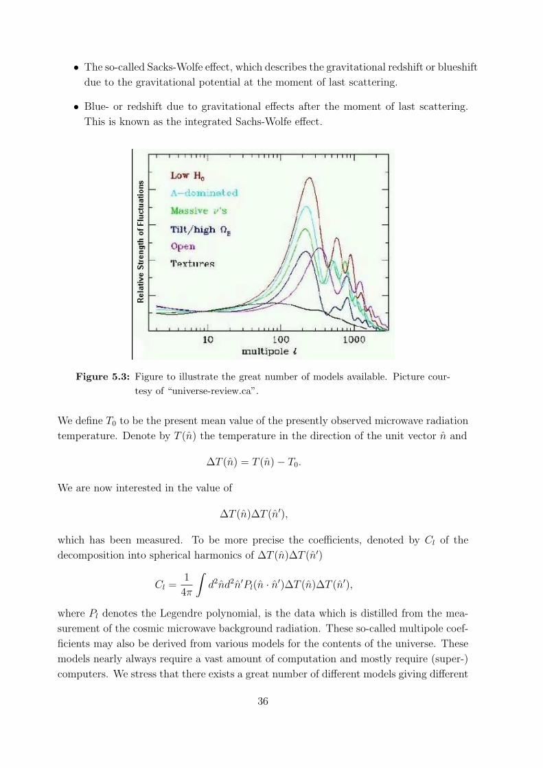
Figure 5.3: Figure to illustrate the great number of models available. Picture cour-tesy of “universe-review.ca”.
We define T0 to be the present mean value of the presently observed microwave radiation
temperature. Denote by T (n) the temperature in the direction of the unit vector n and
∆T (n) = T (n)− T0.
We are now interested in the value of
∆T (n)∆T (n′),
which has been measured. To be more precise the coefficients, denoted by Cl of the
decomposition into spherical harmonics of ∆T (n)∆T (n′)
Cl =1
4π
∫d2nd2n′Pl(n · n′)∆T (n)∆T (n′),
where Pl denotes the Legendre polynomial, is the data which is distilled from the mea-
surement of the cosmic microwave background radiation. These so-called multipole coef-
ficients may also be derived from various models for the contents of the universe. These
models nearly always require a vast amount of computation and mostly require (super-)
computers. We stress that there exists a great number of different models giving different
36
values for the Cls. One may find a figure which compares the results of a popular model,
the so called photon fluid approximation, with observed values. To illustrate the great
number of models available we have also inserted figure 5.3 depicting the results of a
number of models.
37
Acknowledgements
The author would like to thank J. Koksma and T. Procopek for their aid in writing this
report. Moreover the help of J. de Graaf and T. van der Aalst with technical issues is
appreciated.
38
Bibliography
[1] R.H. Brandenberger. Lectures on the Theory of Cosmological Pertubations. ArXiv:
hep-th/0306071v1, 2003.
[2] R.H. Brandenberger, H.A. Feldman, and V.F. Mukhanov. Classical and Quan-
tum Theory of Perpurbations in inflationary Universe Models. ArXiv: astro-
ph/9307016v1, 1993.
[3] C.-P. Ma and E. Bertschinger. Cosmological Pertubation Theory in the Synchronous
and Conformal Newtonian Gauges. ArXiv: astro-ph/9506072v1, 1995.
[4] T. Padmanabhan. Structure Formation in the Universe. Cambridge University
Press, 1993.
[5] P.J.E. Peebles. The Large-scale Structure of the Universe. Princeton University
Press: Princeton, New Jersey.
[6] S. Weinberg. Cosmology. Oxford University Press, 2007.
[7] V.F. Mukhanov, H.A. Feldman, and R.H. Brandenberger. Theory of cosmological