7 Laser-induced Fluorescence Spectroscopy Laser-induced fluorescence (LIF) is (spontaneous) emission from atoms or molecules that have been excited by (laser) radiation. The phenomenon of induced fluorescence was first seen and discussed back in 1905 by R. W. Wood, many decades before the invention of the laser. The process is illustrated schematically in Figure 7.1. If a particle resonantly absorbs a photon from the laser beam, the particle is left in an excited energy state. Such a state is unstable and will decay sponta- neously, emitting a photon again. As has been dis- cussed earlier, the excited state of finite lifetime emits its photon on return to a lower energy level in random directions. It is this fact that allows one to measure an absorption signal directly, as outlined in Chapter 6. Conveniently, the fluorescence is observed at 90 to a collimated laser beam. In principle, a very small focal volume V c may be defined in the imaging set-up, resulting in spatial resolution of the laser–particle interaction volume; note that spatial resolution cannot normally be realized in an experiment, which measures the absorption directly. In a sense, the method of LIF may be seen as a fancy way of measuring the absorption of a species, but with a bonus. Absorption spectroscopy, which detects the transmitted light, has (in many experimental imple- mentations) a limited sensitivity. The problem is that one has to detect a minute amount of missing light in the transmitted beam, i.e. one encounters the problem of the difference of large near-equal numbers. The use of pulsed lasers aggravates the problem due to their normally substantial pulse-to-pulse intensity fluctua- tions, which limit the signal-to-noise ratio. With fluor- escence detection the signal can be detected above a background, which is (at least in favourable cases) nearly equal to zero, and detection at the single- photon level is relatively easy to achieve. As is obvious from the above picture, two radiative transitions are involved in the LIF process. First, absorption takes place, followed by a second photon-emission step. Therefore, when planning a LIF experiment one should always bear in mind that LIF requires considerations associated with absorp- tion spectroscopy. Any fancy detection equipment is merely used to detect the consequences of the absorp- tion, with the additional information on how much was absorbed where. One major caveat with fluorescence measure- ments is that they are no longer associated with a simple absolute measure of the absorbed amount of radiation (and therewith particle concentration). Too many difficult-to-determine or outright unknown factors influence the observed signal. Amongst these factors are spectroscopic quantities, such as quenching, and experimental quantities, such as observation angle and optics transmission, to mention Laser Chemistry: Spectroscopy, Dynamics and Applications Helmut H. Telle, Angel Gonza ´lez Uren ˜a & Robert J. Donovan # 2007 John Wiley & Sons, Ltd ISBN: 978-0-471-48570-4 (HB) ISBN: 978-0-471-48571-1 (PB)
Transcript
7Laser-induced Fluorescence
Spectroscopy
Laser-induced fluorescence (LIF) is (spontaneous)
emission from atoms or molecules that have been
excited by (laser) radiation. The phenomenon of
induced fluorescence was first seen and discussed
back in 1905 by R. W. Wood, many decades before
the invention of the laser. The process is illustrated
schematically in Figure 7.1.
If a particle resonantly absorbs a photon from the
laser beam, the particle is left in an excited energy
state. Such a state is unstable and will decay sponta-
neously, emitting a photon again. As has been dis-
cussed earlier, the excited state of finite lifetime emits
its photon on return to a lower energy level in random
directions. It is this fact that allows one to measure an
absorption signal directly, as outlined in Chapter 6.
Conveniently, the fluorescence is observed at 90� toa collimated laser beam. In principle, a very small
focal volumeVcmay be defined in the imaging set-up,
resulting in spatial resolution of the laser–particle
interaction volume; note that spatial resolution
cannot normally be realized in an experiment, which
measures the absorption directly.
In a sense, themethod ofLIFmaybe seen as a fancy
wayofmeasuring the absorption of a species, butwith
a bonus. Absorption spectroscopy, which detects the
transmitted light, has (in many experimental imple-
mentations) a limited sensitivity. The problem is that
one has to detect a minute amount of missing light in
the transmitted beam, i.e. one encounters the problem
of the difference of large near-equal numbers. The use
of pulsed lasers aggravates the problem due to their
tions,which limit the signal-to-noise ratio.Withfluor-
escence detection the signal can be detected above a
background, which is (at least in favourable cases)
nearly equal to zero, and detection at the single-
photon level is relatively easy to achieve.
As is obvious from the above picture, two radiative
transitions are involved in the LIF process. First,
absorption takes place, followed by a second
photon-emission step. Therefore, when planning a
LIF experiment one should always bear in mind that
LIF requires considerations associated with absorp-
tion spectroscopy. Any fancy detection equipment is
merely used to detect the consequences of the absorp-
tion, with the additional information on how much
was absorbed where.
One major caveat with fluorescence measure-
ments is that they are no longer associated with a
simple absolute measure of the absorbed amount of
radiation (and therewith particle concentration). Too
many difficult-to-determine or outright unknown
factors influence the observed signal. Amongst
these factors are spectroscopic quantities, such as
quenching, and experimental quantities, such as
observation angle and optics transmission, tomention
Laser Chemistry: Spectroscopy, Dynamics and Applications Helmut H. Telle, Angel Gonzalez Urena & Robert J. Donovan# 2007 John Wiley & Sons, Ltd ISBN: 978-0-471-48570-4 (HB) ISBN: 978-0-471-48571-1 (PB)
just a few. Of course, one can describe the fluores-
cence spectral emission quantitatively provided one
knows or can estimate both spectroscopic and experi-
mental parameters that influence it (see Box 7.1).
Despite this analytical shortcoming, its extreme
sensitivity accounts for the popularity of LIF in
many fields, including the investigation of chemical
processes, and for many decades LIF has been one of
the dominant laser spectroscopic techniques in the
probing of unimolecular and bimolecular chemical
reactions.
7.1 Principles of laser-inducedfluorescence spectroscopy
In their simplest form, the processes involved in a LIF
experiment are summarized in Figure 7.2 for a simple
two-level model particle.
If the particle is resonantly stimulated by the laser
source, then a photon of energy h�12 will be absorbed,lifting the particle to the excited state. As is well
known, both stimulated and spontaneous emissions
have to be considered in the temporal decay of the
excited level, where the relative ratio between the two
is determined by the laser intensity. It should be noted
that the stimulated emission process constitutes a loss
mechanism for LIF observation at right angles, as
shown in Figure 7.1, because those photons propagate
in the direction of the incoming laser beam. A further
loss to the signal tobeobserved is related tocollisional
quenching of the excited energy level, without the
emission of a photon. Although quenching may not
be a problem in high-vacuum conditions, where the
time between collisions is normally much longer
than the radiative lifetime, many experiments are
run under conditions in which collisional quenching
is important; this will be discussed further in some of
the examples given below.
It also should be noted that scattered light at the same
wavelength as the excitation light may obscure a fluor-
escence signal if the latter is also observed on the same
downwardtransitionwavelengthas theexcitation.How-
ever, with suitably fast detection electronics one can
distinguish between the two: scattering occurs instanta-
neously, whereas the duration of the fluorescence signal
depends on the lifetime of the upper energy level.
As the species looked at in chemical reactions are
mostly molecules, the two electronic levels depicted
in Figure 7.2 split into sub-levels, according to the
molecular vibrational and rotational energy quanta.
The vibrational levels are customarily numberedwith
the quantum number viði ¼ 0, 1, 2,...). The notation
for the rotational levels is more complex and depends
as well on the size of the molecule, but typically one
associates the rotation with the quantum number
Jiði ¼ 0, 1, 2,...). In order to distinguish between
states, double primes are used to mark the (lower)
ground-state levels and single-primed quantum num-
bers mark the excited (upper) state levels. The main
The absorption starts at a distinct rotational and
vibrational level within the lower electronic (ground)
IL(ν)
Nbuffer
Ntrace
Fluorescence IF(νF)
Scattered light IR(ν)
photodetector
lens
Figure 7.1 Principle of fluorescence emission, IFðvF),from particles in a gas mixture, after absorption of tune-able laser light ILðvÞ. Scattered light IRðvÞ at the samefrequency as the incoming laser light is also observed
N1·B12·I(ν) N2·Q
absorption stimulatedemission
E1
E2
N1(t)
N2(t)
hν = E2-E1
N = N1(t)+N2(t)
fluorescence quenching
N2·B2·I(ν) N2·A21
Figure 7.2 Radiative and non-radiative processes in atwo-level system
102 CH7 LASER-INDUCED FLUORESCENCE SPECTROSCOPY
Box 7.1
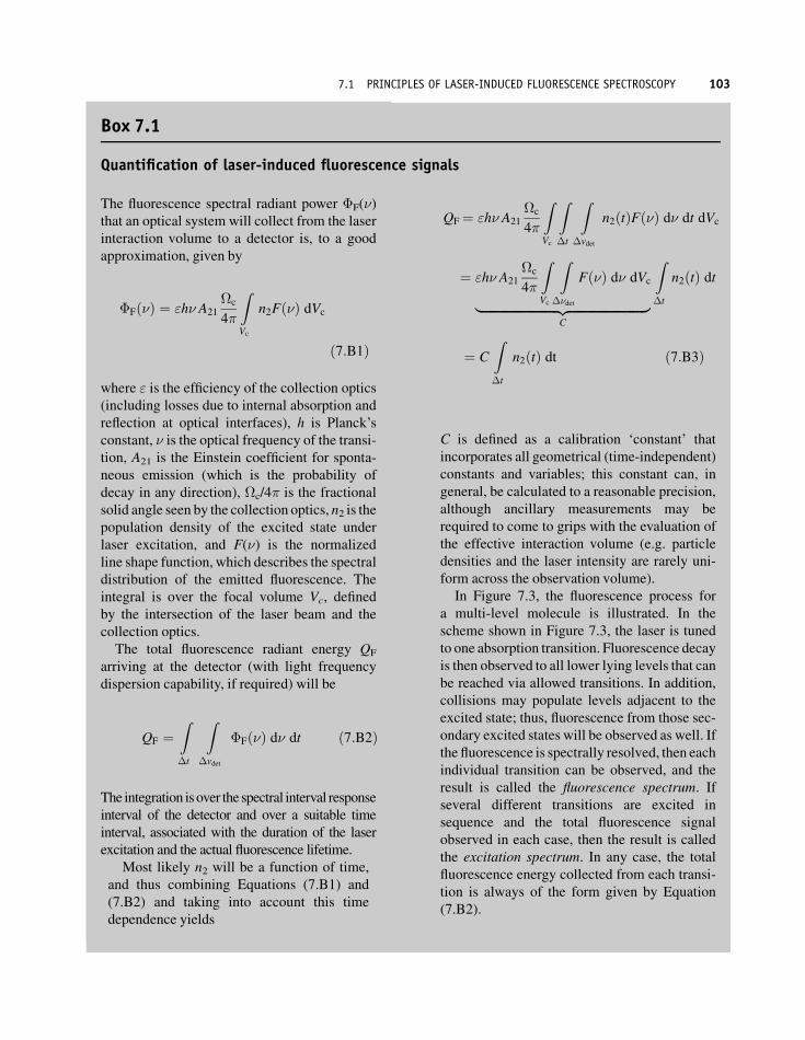
Quantification of laser-induced fluorescence signals
The fluorescence spectral radiant power �F(�)that an optical system will collect from the laser
interaction volume to a detector is, to a good
approximation, given by
�Fð�Þ ¼ "h� A21
�c
4�
ZVc
n2Fð�Þ dVc
ð7:B1Þ
where " is the efficiency of the collection optics(including losses due to internal absorption and
reflection at optical interfaces), h is Planck’s
constant, � is the optical frequency of the transi-tion, A21 is the Einstein coefficient for sponta-
neous emission (which is the probability of
decay in any direction), �c/4� is the fractional
solid angle seen by the collection optics, n2 is the
population density of the excited state under
laser excitation, and F(�) is the normalized
line shape function, which describes the spectral
distribution of the emitted fluorescence. The
integral is over the focal volume Vc, defined
by the intersection of the laser beam and the
collection optics.
The total fluorescence radiant energy QF
arriving at the detector (with light frequency
dispersion capability, if required) will be
QF ¼Z�t
Z�vdet
�Fð�Þ d� dt ð7:B2Þ
The integration isover the spectral interval response
interval of the detector and over a suitable time
interval, associated with the duration of the laser
energy difference between the two levels is associated
with the energy of the incident photon. Emission from
the excited quantum state is possible to all lower lying
energy levels, to which transitions are allowed, gov-
erned by the quantum selection rules for electronic
dipole transitions (see Chapter 2). By and large one
findsamultitudeofemissionlines; their intensitiesmay
be measured globally (integration of the whole
light intensity) or individually. Both methods provide
useful information, as will be discussed in Section 7.2.
In addition to the non-radiative quenching men-
tioned further above, an addition collisional energy
transfer process can be observed, namely the transfer
from the laser-excited level to neighbouring quantum
levels within the excited-state manifold. Hence, under
the right conditions, one observes lines from levels that
were not directly populated by the laser excitation.
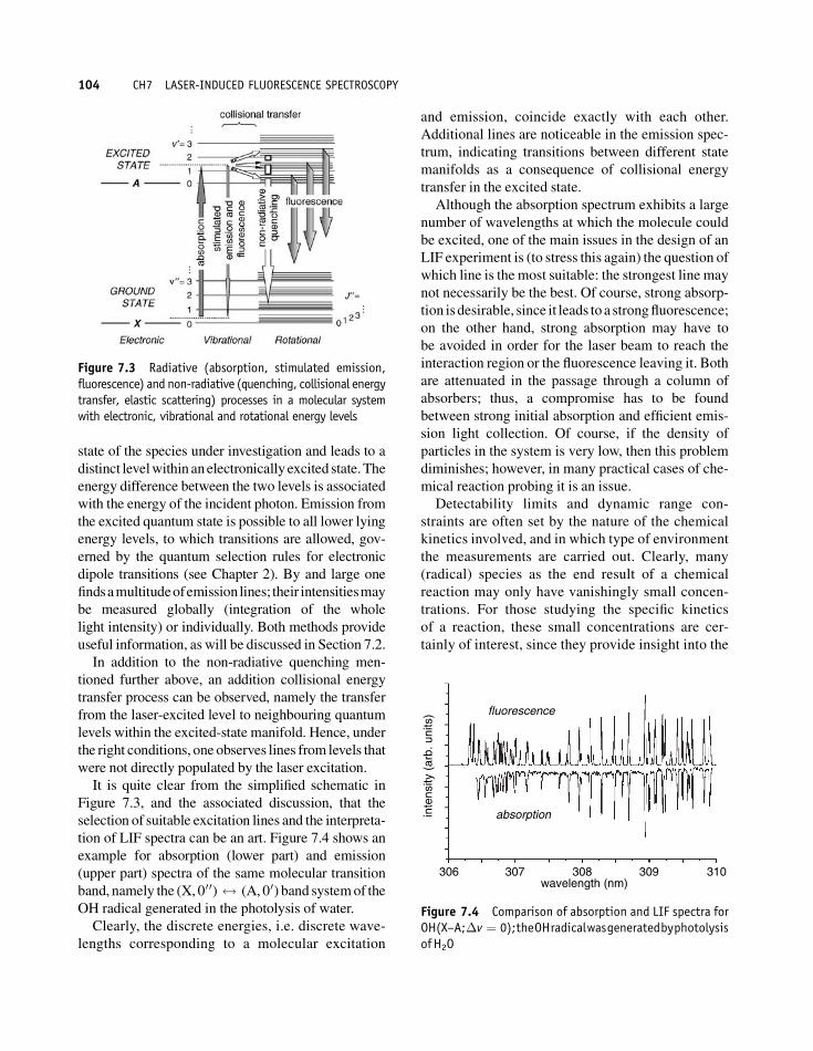
It is quite clear from the simplified schematic in
Figure 7.3, and the associated discussion, that the
selection of suitable excitation lines and the interpreta-
tion of LIF spectra can be an art. Figure 7.4 shows an
example for absorption (lower part) and emission
(upper part) spectra of the same molecular transition
band, namely the (X, 000) $ (A, 00) band systemof the
OH radical generated in the photolysis of water.
Clearly, the discrete energies, i.e. discrete wave-
lengths corresponding to a molecular excitation
and emission, coincide exactly with each other.
Additional lines are noticeable in the emission spec-
trum, indicating transitions between different state
manifolds as a consequence of collisional energy
transfer in the excited state.
Although the absorption spectrum exhibits a large
number of wavelengths at which the molecule could
be excited, one of the main issues in the design of an
LIF experiment is (to stress this again) the question of
which line is the most suitable: the strongest line may
not necessarily be the best. Of course, strong absorp-
tion isdesirable, since it leads toa strongfluorescence;
on the other hand, strong absorption may have to
be avoided in order for the laser beam to reach the
interaction region or the fluorescence leaving it. Both
are attenuated in the passage through a column of
absorbers; thus, a compromise has to be found
between strong initial absorption and efficient emis-
sion light collection. Of course, if the density of
particles in the system is very low, then this problem
diminishes; however, in many practical cases of che-
mical reaction probing it is an issue.
Detectability limits and dynamic range con-
straints are often set by the nature of the chemical
kinetics involved, and in which type of environment
the measurements are carried out. Clearly, many
(radical) species as the end result of a chemical
reaction may only have vanishingly small concen-
trations. For those studying the specific kinetics
of a reaction, these small concentrations are cer-
tainly of interest, since they provide insight into the
fluorescence
absorption
306 307 308 310309wavelength (nm)
inte
nsity
(ar
b. u
nits
)
Figure 7.4 Comparison of absorption and LIF spectra forOH(X–A;�v ¼ 0);theOHradicalwasgeneratedbyphotolysisof H2O
Figure 7.3 Radiative (absorption, stimulated emission,fluorescence) and non-radiative (quenching, collisional energytransfer, elastic scattering) processes in a molecular systemwith electronic, vibrational and rotational energy levels
104 CH7 LASER-INDUCED FLUORESCENCE SPECTROSCOPY
global picture of branching into reaction channels.
However, from a practical point of view (e.g. in an
industrial production process) there is usually some
limit below which the concentration of a species is
insignificant with regard to the overall process. On
the other hand, if one includes the detection of
hazardous compounds in the environment as an
object of study by LIF, then the range of concentra-
tions over which measurement is desirable may be
indeed extremely small, down to concentrations of
parts per trillion (ppt).
7.2 Important parameters inlaser-induced fluorescence
Theoverallaimintheinvestigationofreactiondynamics
of chemical processes is to obtain a detailed picture of
the path (or paths) that links reactants to products in a
chemical reaction, as will be discussed in great detail in
Parts 4 and 5. The ‘dynamics’ of a reaction can be
characterized by measurements of some or all of the
following important aspects (not a complete list):
� Reagent properties. In which way is the reaction
influenced by properties such as reagent quantum
state, velocity or light polarization (which induces
spatial orientation of the particle in resonance with
the radiation)?
� Product quantum state.Does one observe recogniz-
able deviations from a thermal level population
distribution (both vibration and rotation)?
� Product velocity distribution. Is the collision energychannelled into product translation and/or internal
excitation?
� Product angular distribution. Are the observed pro-
through a complex intermediate, and/or is the pro-
duct affected by predissociation?
These questions may be addressed if reactions are
studied with product state resolution, under single
collision conditions (i.e. products are detected
before they can undergo secondary collisions, so
that their motion is characteristic of the forces
experienced during the reaction). Then one can
often work backwards from the measured product
parameters to infer the processes that must have
occurred during the reactive collision. Thus, one
gains insight into the forces and energetics govern-
ing the reaction, associated with the particular
potential energy surfaces (PESs) for the reaction.
Some of these parameters and their measurement,
and what can be learned from the data, are described
in more detail below.
Product quantum state informationderived from laser-inducedfluorescence measurements
The LIF signal can be used in a number of ways.Most
simply, it provides a measure of the population of the
excited state (or states) through Equation (7.B3)
deduced in Box 7.1. In addition, if a relationship can
be foundbetween the number densities of all quantum
states involved in the excitation–emission sequence,
then the total number density of the species can be
deduced. However, a further wealth of information
can be extracted from the LIF signals. As pointed out
above, there are twobasic approaches to the recording
of LIF spectra. In the first, one excites the species
under investigation in a single quantum transition
and records the emission utilizing a wavelength-
selective detection system, commonly known as the
fluorescence spectrum. In the second, one tunes the
exciting laser across all transitions accessible within
its spectral range and records the fluorescence glob-
ally (integrated over all emission wavelengths); the
result is known as the excitation spectrum.
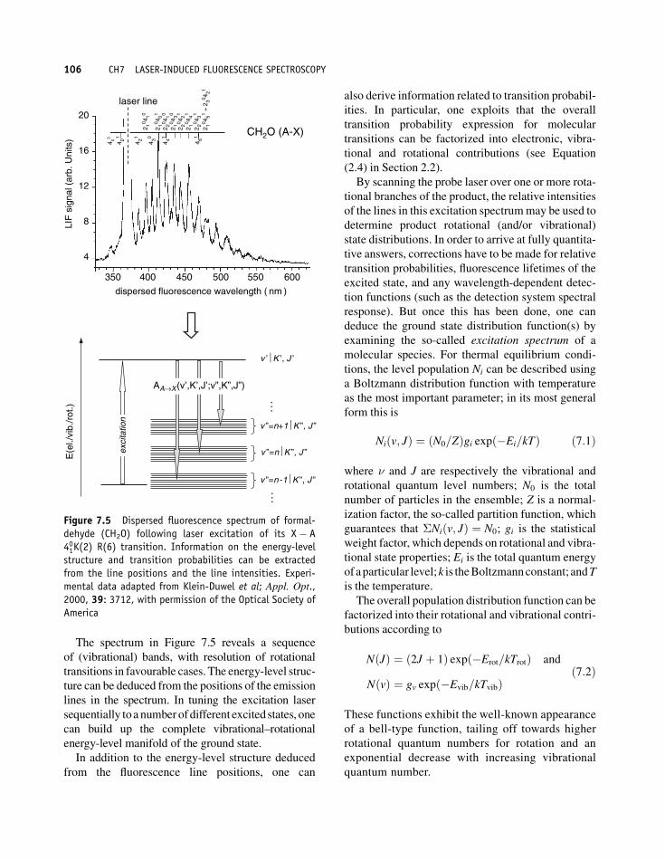
Anexample for afluorescence spectrumis shown in
Figure 7.5 for the molecule CH2O; note the strong
signal at the wavelength of the laser excitation line,
which amplifies the argument that, in order to elim-
inate the contribution of scattered light to the LIF
spectrum, observation conveniently should be
done at a wavelength different from the excitation.
Fortunately, because of the vibrational–rotational
energy-level manifolds encountered in molecules,
this can mostly be realized.
7.2 IMPORTANT PARAMETERS IN LASER-INDUCED FLUORESCENCE 105
The spectrum in Figure 7.5 reveals a sequence
of (vibrational) bands, with resolution of rotational
transitions in favourable cases. The energy-level struc-
ture can be deduced from the positions of the emission
lines in the spectrum. In tuning the excitation laser
sequentially toa numberofdifferent excited states, one
can build up the complete vibrational–rotational
energy-level manifold of the ground state.
In addition to the energy-level structure deduced
from the fluorescence line positions, one can
also derive information related to transition probabil-
ities. In particular, one exploits that the overall
transition probability expression for molecular
transitions can be factorized into electronic, vibra-
tional and rotational contributions (see Equation
(2.4) in Section 2.2).
By scanning the probe laser over one or more rota-
tional branches of the product, the relative intensities
of the lines in this excitation spectrummay be used to
determine product rotational (and/or vibrational)
state distributions. In order to arrive at fully quantita-
tive answers, corrections have to be made for relative
transition probabilities, fluorescence lifetimes of the
excited state, and any wavelength-dependent detec-
tion functions (such as the detection system spectral
response). But once this has been done, one can
deduce the ground state distribution function(s) by
examining the so-called excitation spectrum of a
molecular species. For thermal equilibrium condi-
tions, the level population Ni can be described using
a Boltzmann distribution function with temperature
as the most important parameter; in its most general
form this is
Niðv; JÞ ¼ ðN0=ZÞgi expð�Ei=kTÞ ð7:1Þ
where � and J are respectively the vibrational and
rotational quantum level numbers; N0 is the total
number of particles in the ensemble; Z is a normal-
ization factor, the so-called partition function, which
guarantees that �Niðv; JÞ ¼ N0; gi is the statistical
weight factor, which depends on rotational and vibra-
tional state properties; Ei is the total quantum energy
of aparticular level;k is theBoltzmannconstant; andT
is the temperature.
The overall population distribution function can be
factorized into their rotational and vibrational contri-
butions according to
NðJÞ ¼ ð2J þ 1Þ expð�Erot=kTrotÞ and
NðvÞ ¼ gv expð�Evib=kTvibÞð7:2Þ
These functions exhibit the well-known appearance
of a bell-type function, tailing off towards higher
rotational quantum numbers for rotation and an
exponential decrease with increasing vibrational
quantum number.
LIF
sig
nal (
arb.
Uni
ts)
CH2O (A-X)
204 03
4 01
4 21
2 10 4
10
2 10 4
01
2 20 4
10
2 10 4
30
2 20 4
21
2 10 4
41
2 20 4
31
2 10 4
51 +
230 4
21
4 30
4 61
4 41
16
12
8
4
350 400 450 500 550 600
dispersed fluorescence wavelength ( nm )
laser line
v ”=n+1K ”, J ”
v ”=n -1K ”, J ”
v ”=nK ”, J ”
v ’K ’, J ’
AA→X(v’,K’,J’;v”,K”,J”)
exci
tatio
n
E(e
l./vi
b./r
ot.)
Figure 7.5 Dispersed fluorescence spectrum of formal-dehyde (CH2O) following laser excitation of its X� A401K(2) R(6) transition. Information on the energy-levelstructure and transition probabilities can be extractedfrom the line positions and the line intensities. Experi-mental data adapted from Klein-Duwel et al; Appl. Opt.,2000, 39: 3712, with permission of the Optical Society ofAmerica
106 CH7 LASER-INDUCED FLUORESCENCE SPECTROSCOPY
An example for the principle of extracting a dis-
tribution function from an LIF spectrum is shown in
Figure 7.6.
It should be noted that the observed distribution
functions might not be thermal. In fact, for a large
number of product state distributions from uni- and
bi-molecular reactions, one observes significant
deviations form the Boltzmann functions, which
reflect particular state-to-state chemical reaction
dynamics.
It should also be noted that, with knowledge of
the results from LIF experiments, which provide
the energy-level structure and population information
in a particular molecular state, one is able to simulate
electronic transitions and their ro-vibrational bands
from the derived spectroscopic parameters. An
example for this procedure is shown in Figure 7.7;
here, the simulated spectrum of the SrF(X–B) transi-
tion bands matches the observations extremely well,
even reproducing the undulating feature of rotational
state interference, when they coincide, or not, at the
same wavelength position.
Study of individual laser-inducedfluorescence transition lines
In general, the species under observation, the exci-
tation system, and the detection system all have
different line widths associated with them. Nor-
mally, one finds that ��det � ��mol, ��las for therelated widths parameters. The relative relation
between the latter two depends very much on
whether the laser is a pulsed laser or a CW laser;
the half-width of a nanosecond-duration pulsed
laser is normally much larger than the Doppler
profile of the atom or molecule, whereas the oppo-
site holds for CW lasers.
Thus, using a narrow-bandwidth laser, in addition
to quantum-state-resolved measurements of the pro-
duct, one can access the velocity and angularmomen-
tum distributions by making detailed measurements
on a single rotational transition line. The transition is
scanned at high resolution to resolve the Doppler line
shape, effectively providing a 1D projection of the
particle velocity along the probe laser propagation
direction. Ultimately, by repeating such a measure-
ment in different geometries, full 3 D spatial velocity
distributions could be derived. This could be
done both for reagents and for products in a chemical
reaction.
For example, by measuring the Doppler profile in
the direction of an atomic or molecular beam, and
perpendicular to it, one can determine the transla-
tional energy contribution to a reaction. An example
for such a measurement is shown in Figure 7.8.
Clearly, the average velocity in the propagation
direction of the beam is much larger than the dis-
tribution in the perpendicular coordinate; from the
longitudinal velocity component, the kinetic energy
Figure 7.6 LIF excitation spectrum for the CuI(C, �0 ¼0�X, �00 ¼ 0) band, with rotational line resolution,originating from the molecular beam reaction Cu þ I2 !CuI þ I . Level population information can be extractedfrom the spectral intensities (bottom). Experimental dataadapted from Fang and Parson, J. Chem. Phys., 1991, 95:6413,with permission of theAmerican Institute of Physics
7.2 IMPORTANT PARAMETERS IN LASER-INDUCED FLUORESCENCE 107
Ekin ¼ 12mv2 in a subsequent reactive collision can
be derived.
A similar velocity-measuring experiment can
be carried out, for example, for product mole-
cules. But, instead of physically altering the pro-
pagation direction of the laser beam, one may
exploit that different experimental geometries
are also defined by the relative orientation of the
laser propagation plus its polarization directions,
and the particle movement. A sufficient number
of related one-dimensional velocity projections
allow for the reconstruction of a full 3 D velocity
distribution. Information on angular momentum
alignment can also be extracted because the
transition probability depends on the relative
orientation of the laser polarization and the total
angular momentum vector of the probed product.
An example for this type of 3 D velocity profile
reconstruction is shown in Figure 7.9 for the
example of OH generated as a product in the
reaction Hþ N2O! OHþ NO (Brouard et al.,
2002). In this particular example, the results
allowed the researchers to conclude from the
stereodynamic reconstruction that the OH product
was back scattered and that the reaction proceeded
via a complex intermediate.
Figure 7.7 Experimental (a) and calculated (b) LIF spectra of SrF(B–X; �v ¼ 0), formed in the reaction Sr*(3P1)þ HF,for spectral resolution of 0.4 cm�1. The wiggle-like structure seen at the long-wavelength side is due to partially resolvedrotational lines in the tail of the R-branches. Reproduced form Teule et al; J. Chem. Phys., 1998,102: 9482, with permission ofthe American Institute of Physics
150010005000-500
0.0
0.2
0.4
0.6
0.8
1.0
v (m·s-1)
3000 100 200
v0 ≅ 960 m/s
(v − v0)2
2σ2f(v) = v2 ⋅exp
−
LIF
inte
nsity
(re
l. un
its)
dn (MHz)
Figure 7.8 Transverse and longitudinal velocity dis-tribution of Ca atomic beam, derived from the LIF responseinduced by a narrow-bandwidth CW dye laser (�vL �5MHz)
108 CH7 LASER-INDUCED FLUORESCENCE SPECTROSCOPY
Pressure and temporal aspects inlaser-induced fluorescence emission
In order to realize easily observable products from
chemical reactions, the number density of reagents
and subsequent products needs to be sufficiently high
so that laser spectroscopic techniques generate mea-
surable signals. However, with increasing number
density, or gas pressure, secondary effects beyond
that of the original reaction are observed.Specifically,
in LIF experiments, the excited-state lifetime can be-
come longer than theaverage timebetweencollisions.
This will influence this fluorescing state, resulting in
apparent shortening of the lifetime, broadening of the
transition line profile, and reduction in the LIF signal
amplitude. Although this is frequently seen as an
annoying effect in an LIF experiment, it may actually
be used to derive important parameters of the reaction
itself or about the interaction of a particularmolecular
state with its environment. Thus, experiments are
often designed to follow the collisional effects as a
function of gas pressure.
When the particle density is sufficiently small that
the simple spontaneous decay equation for the excited
state once the excitation laser pulse is over. Thus,
plotting the fluorescence intensity, on a logarithmic
scale, against timewill result in apparent linear depen-
dence, and the lifetime is calculated from the slope of
the resulting line (see Figure 7.10a).
If, on the other hand, the fluorescence lifetime is
shorter than or of the same order as the excitation
pulse, then the decay must be deconvolved from the
excitation pulse, because the overall fluorescence
signal response is represented, to a good approx-
imation by
IL � IF /ðILðt � t0ÞniðtÞ expð�t=tÞ dt ð7:3Þ
A + BC AB(J) + C
pv
v
-1 0 1
-1 0 1 -1 0 1
–1 0 1
2
1
0
2
1
0
2
1
0
2
1
0
Doppler shift / cm–1
–45º 0º
+45º90º
Figure 7.9 Raw experimental Doppler profile LIF data of theproduct state OH(X; v0 ¼0, J0 ¼5), for different laser light polar-izationdirections (clockwise fromtop�45�, 0�, 45�, 90�),whichare converted into 3D velocity–angle polar plots of the productscattering distribution. Information on the reaction stereody-namicscanbeextractedfromthedata.Experimentaldataadaptedwith permission from Brouard et al, J. Phys. Chem. A 106: 3629.Copyright 2002 American Chemical Society
7.2 IMPORTANT PARAMETERS IN LASER-INDUCED FLUORESCENCE 109
where t0 is the time when the laser pulse commences
(or anyother convenient time reference), and� repre-
sents the convolution operator. A common algorithm
for retrieving the lifetime in this case is the method of
least-squares iterative re-convolution: the (known)
excitation pulse is convolved with an exponential
decay function of varying lifetime parameter until
that parameter most closely matches the emission
data (see Figure 7.10b).
As soon as collisions start to occur on a scale
comparable to the radiative lifetime, the evolution
of the upper state population is affected. The life-
time of a transition is apparently shortened. This
shortening can be associated with the rate of quench-
ing collisions and one arrives at an effective lifetime
equation
t�1eff ¼ t�1 þ kQðp; TÞ þ kD ð7:4Þ
where kQðp; TÞ (s�1) is the quenching rate, which
depends on the pressure and temperature of the colli-
sion gas. Note that the quenching rate is often ex-
pressed in the form kQ ¼ kqp, where kq (cm3 s�1) is
the pressure-independent quenching coefficient and p
(cm�3) is thepressureexpressed in termsof theparticle
number density. The final factor, kD, is associatedwith
a possible predissociation rate for particular energy
levels (see further below). An example of how the
measurement of the collision-affected lifetime can
result in useful information is shown in Figure 7.11.
First, fromplotting thefluorescence lifetimedata in
the form t�1eff versus pressure, one can extract the
natural radiative lifetime. This is useful in cases for
which no collision-free environment can be realized.
Second, from the slope of the plot one can extract
the quenching rate constant kQ, which in itself is
associated with the quenching cross-section of the
Figure 7.10 LIF lifetime measurements, following an excitation laser pulse of duration�t ffi 4:5 ns FWHM. If the lifetimeof theexcited level is longer than theexcitationpulse, then the lifetimecanbeextracted fromthe slopeof the semi-logarithmicplot (trace a); if the radiative lifetime signal is detected with electronics of similar time constants, then RC-responsedeconvolution needs to be applied (trace b); and if the lifetime is of similar length or slightly shorter than the laser pulse,full line shape function deconvolution procedures are required (trace c). Data shown in trace (b) are adapted fromVerdasco et al; Laser Chem., 1990, 10: 239, with permission of Taylor & Francis Group
110 CH7 LASER-INDUCED FLUORESCENCE SPECTROSCOPY
collision �quench; both parameters are commonly used
in the description of chemical reaction processes. It
should be noted that, in general, one will be unable to
conclude froma simple plot like the one inFigure 7.11
whether the quenching of the excited-state population
is due to non-radiative deactivation or a consequence
of a chemical reaction; additional measurements are
normally required.
Such additional measurements can, for example,
take the formof the data shown inFigure 7.12.A set of
LIF intensity data for a beam–gas reaction is plotted
against gas pressure in the chemical reaction (and
probe) volume for the specific case of the reactive
collision
Cað1S0; 3PJ ; 1D2Þ þ Cl2 ! CaClðX;A;BÞ þ Cl
In addition to the LIF-attenuation data for the Ca
reagent atom in its various excitation levels, data for
the yield of the reactive channel into electronically
100 0 300 200 500400 time (ns)
10
5
0
LIF
inte
nsity
(ar
b. U
nits
)
OH (A,v’=1 – X,v”=0)λexc ≅ 283 nm
τ eff–1
τ0–1
pressure
slope ∝ kQ(p,T ) ∝ σquench
0
0.7 mbar
2 mbar
207 ± 1 ns
85.3 ± 0.3 ns
Figure 7.11 LIF signal decay of OH(A, v0 ¼ 1), afterexcitation from (X, v00 ¼ 0) at l ffi 283 nm, as a function oftime. Information on the quenching cross-section can beextracted from the measured effective life times fordifferent pressures. Note that t�1eff ¼ t�1 þ kQðp; TÞ þ kP,with t�1 ¼ Aji the spontaneous emission rate, kQ(p, T ) isthe collisional quenching rate, and kP is the predissociationrate
Figure 7.12 LIF probingof the reagent atomand simulta-neousmeasurement of the total product fluorescence in thereaction Ca/Ca*þCl2 !CaCl (X, A, B)þ Cl, as a function of(reactive) gas pressure. Information on total and reactivecross-sections can be extracted from the data (�r and �
�r :
reaction cross-sections into ground and excited products;�Q: quenching cross-section; �S: elastic scattering cross-section)
7.2 IMPORTANT PARAMETERS IN LASER-INDUCED FLUORESCENCE 111
excited products, Ca�(A, B), were monitored via
their chemiluminescence emission; and for the
‘dark’ channel, CaCl(X) LIF excitation spectra were
recorded (not shown). By combining information
from all data plots, the individual components of
the total quenching cross-section
�tot ¼ �r þ ��r þ �Q þ �Scan be extracted. Here, �r and �
�r are the reaction
cross-sections into ground- and excited-state pro-
ducts, �Q is the non-radiative quenching cross-
section, and �S is the (elastic and/or inelastic) scatter-ing cross-section. The latter can be measured
by probing for the presence of reagent and pro-
duct states outside the interaction volume, or by the
appearance of fluorescence from energy levels that
werenotdirectlypopulatedby the laser excitation.For
comparison, attenuation data for the non-reactive col-
lision Ca� þ N2 are included, which clearly underpin
the notion that the other collisions are indeed effi-
ciently yielding reaction products.
Predissociation probed by laser-inducedfluorescence
The final topic addressed in this section is that of
predissociation of molecules. It is the interaction
between energy level configurations, which initiate
the transfer from one (chemically stable) state to
another (chemically unstable) state. The difference
with respect to photon interaction promoting the
molecule from a lower to a higher energy level is
that the predissociation interaction is a molecule-
internal quantum process. Predissociation after an
excitation can be detected in a number of ways, e.g.
including the appearance of a daughter product or
the unexpected disappearance (cut-off) of lines in a
rotational/vibrational band sequence. The latter is
normally easy to recognize and it does not require
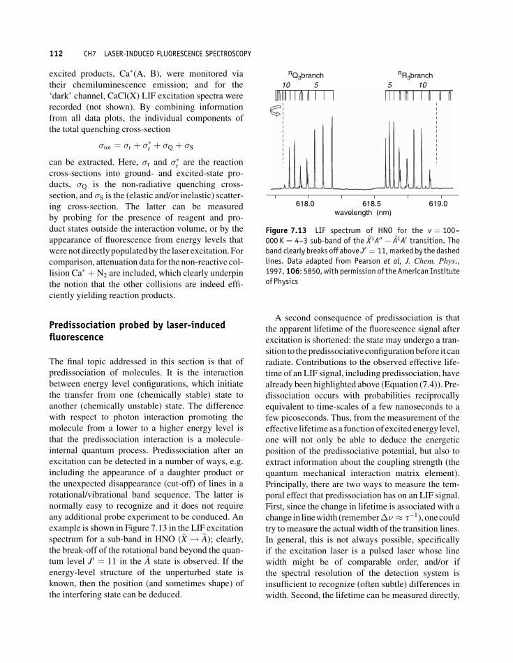
any additional probe experiment to be conduced. An
example is shown in Figure 7.13 in the LIF excitation
spectrum for a sub-band in HNO (~X ! ~A); clearly,the break-off of the rotational band beyond the quan-
tum level J0 ¼ 11 in the ~A state is observed. If the
energy-level structure of the unperturbed state is
known, then the position (and sometimes shape) of
the interfering state can be deduced.
A second consequence of predissociation is that
the apparent lifetime of the fluorescence signal after
excitation is shortened: the state may undergo a tran-
sition to thepredissociativeconfigurationbefore it can
radiate. Contributions to the observed effective life-
time of an LIF signal, including predissociation, have
already been highlighted above (Equation (7.4)). Pre-
dissociation occurs with probabilities reciprocally
equivalent to time-scales of a few nanoseconds to a
few picoseconds. Thus, from the measurement of the
effective lifetimeas a function of excited energy level,
one will not only be able to deduce the energetic
position of the predissociative potential, but also to
extract information about the coupling strength (the
quantum mechanical interaction matrix element).
Principally, there are two ways to measure the tem-
poral effect that predissociation has on an LIF signal.
First, since the change in lifetime is associated with a
change in linewidth (remember�� � t�1), onecouldtry to measure the actual width of the transition lines.
In general, this is not always possible, specifically
if the excitation laser is a pulsed laser whose line
width might be of comparable order, and/or if
the spectral resolution of the detection system is
insufficient to recognize (often subtle) differences in
width. Second, the lifetime can be measured directly,
618.0 618.5 619.0wavelength (nm)
10 5 5 10
RQ3branch RR3branch
Figure 7.13 LIF spectrum of HNO for the v ¼ 100--000 K ¼ 4--3 sub-band of the ~X1A00 � ~A1A0 transition. Theband clearly breaks off above J0 ¼ 11,marked by the dashedlines. Data adapted from Pearson et al, J. Chem. Phys.,1997,106: 5850,with permission of the American Instituteof Physics
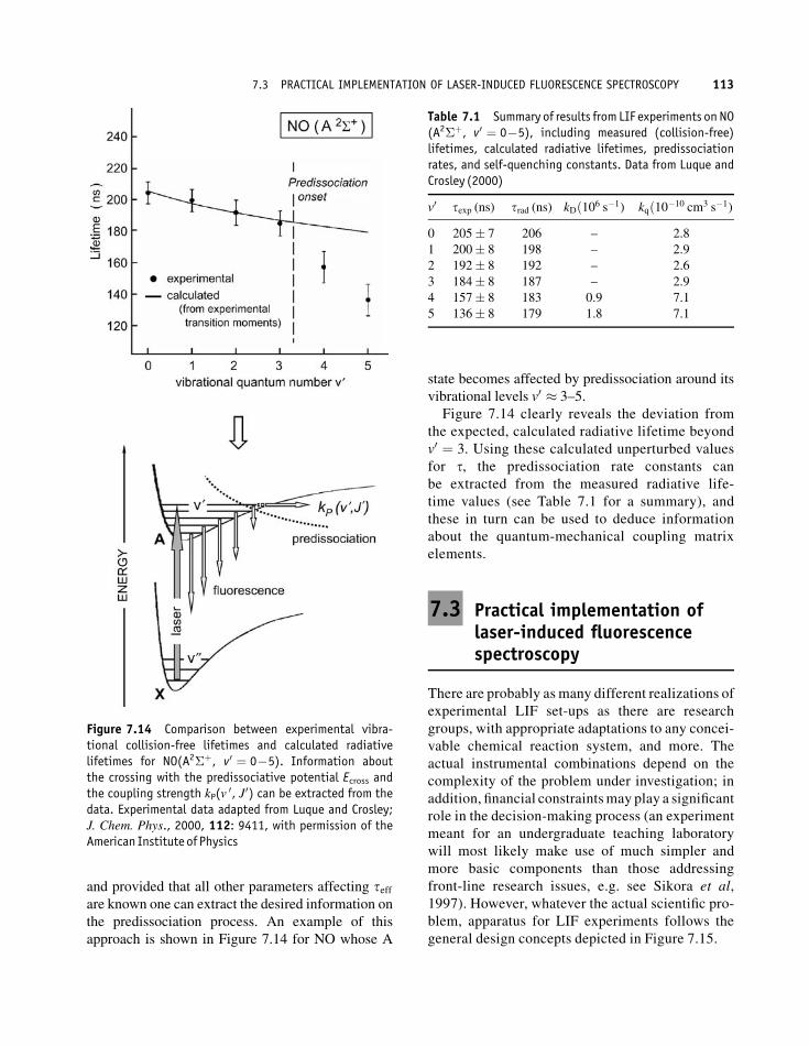
112 CH7 LASER-INDUCED FLUORESCENCE SPECTROSCOPY
and provided that all other parameters affecting teffare known one can extract the desired information on
the predissociation process. An example of this
approach is shown in Figure 7.14 for NO whose A
state becomes affected by predissociation around its
vibrational levels v0 � 3–5.
Figure 7.14 clearly reveals the deviation from
the expected, calculated radiative lifetime beyond
There are probably as many different realizations of
experimental LIF set-ups as there are research
groups, with appropriate adaptations to any concei-
vable chemical reaction system, and more. The
actual instrumental combinations depend on the
complexity of the problem under investigation; in
addition, financial constraintsmay play a significant
role in the decision-making process (an experiment
meant for an undergraduate teaching laboratory
will most likely make use of much simpler and
more basic components than those addressing
front-line research issues, e.g. see Sikora et al,
1997). However, whatever the actual scientific pro-
blem, apparatus for LIF experiments follows the
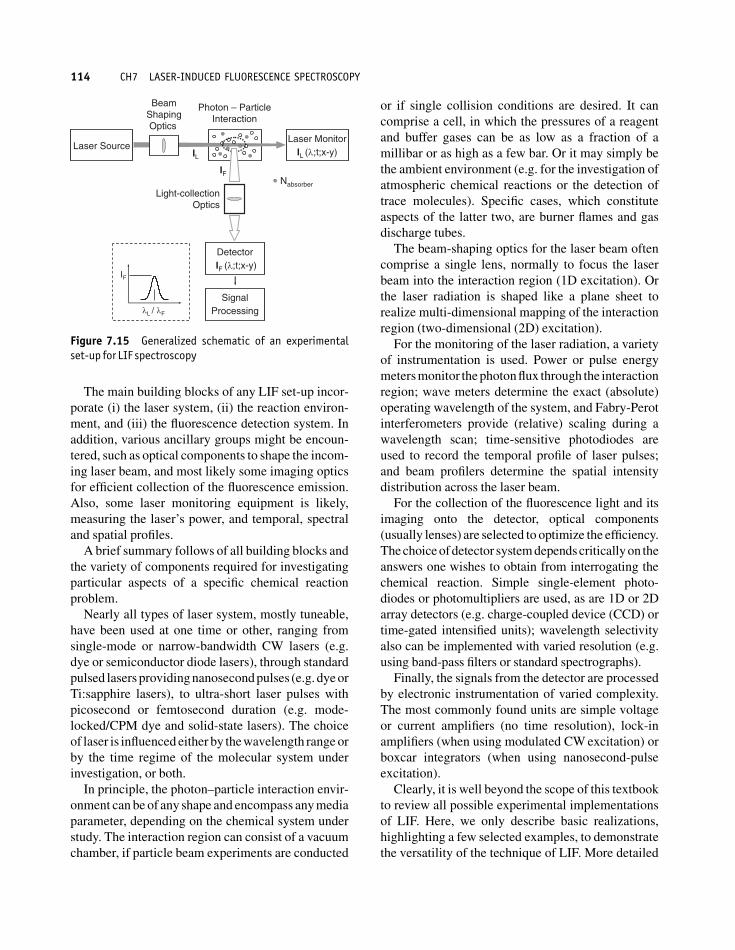
general design concepts depicted in Figure 7.15.
Figure 7.14 Comparison between experimental vibra-tional collision-free lifetimes and calculated radiativelifetimes for NO(A2�þ, v0 ¼ 0�5). Information aboutthe crossing with the predissociative potential Ecross andthe coupling strength kP(v
0, J0) can be extracted from thedata. Experimental data adapted from Luque and Crosley;J. Chem. Phys., 2000, 112: 9411, with permission of theAmerican Institute of Physics
Table 7.1 Summary of results from LIF experiments on NO(A2�þ, v0 ¼ 0�5), including measured (collision-free)lifetimes, calculated radiative lifetimes, predissociationrates, and self-quenching constants. Data from Luque andCrosley (2000)
Probably the most utilized of experimental set-ups
since the conception of LIF is that of a collimated or
focused laser beam (from a pulsed or CW laser)
passing through a region inwhich a chemical reaction
(uni- or bi-molecular) is taking place. That region can
be the interior of a simple vapour cell, a molecular
beam, a beam–gas arrangement, or the configuration
of crossed molecular beams, and the environment
in that reaction region may realize collision-free or
collision-dominated conditions for the LIF probe. A
typical example for a crossed molecular beam LIF
apparatus is shown in Figure 7.16.
The system comprises a vacuum chamber with a
molecular beam source at one end. The particle beam
of reagents and/or products is interrogated in an obser-
vation region (in which reactions may be initiated by a
reagent gas), at right angles, by pulses from a tuneable
laser source. The LIF emission is monitored perpendi-
cular totheplaneformedbytheparticleandlaserbeams.
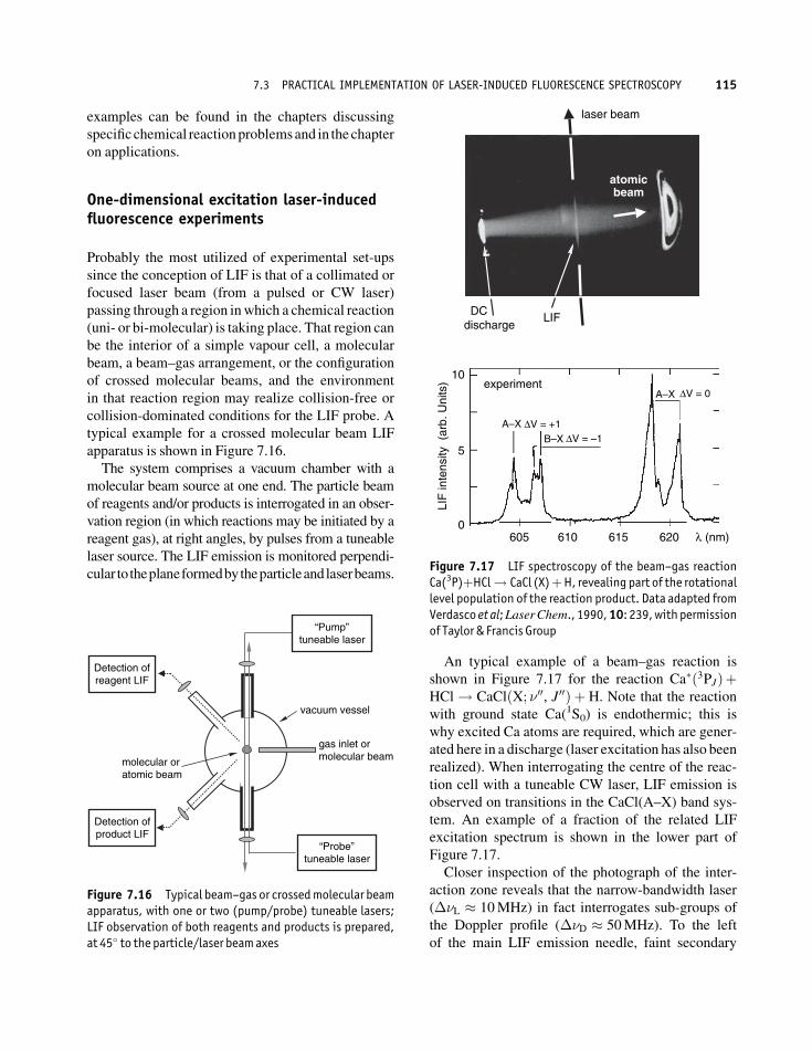
An typical example of a beam–gas reaction is
shown in Figure 7.17 for the reaction Ca�ð3PJÞþHCl! CaClðX; �00, J00Þ þ H. Note that the reaction
with ground state Ca(1S0) is endothermic; this is
why excited Ca atoms are required, which are gener-
ated here in a discharge (laser excitation has also been
realized). When interrogating the centre of the reac-
tion cell with a tuneable CW laser, LIF emission is
observed on transitions in the CaCl(A–X) band sys-
tem. An example of a fraction of the related LIF
excitation spectrum is shown in the lower part of
Figure 7.17.
Closer inspection of the photograph of the inter-
action zone reveals that the narrow-bandwidth laser
(��L � 10MHz) in fact interrogates sub-groups of
the Doppler profile (��D � 50MHz). To the left
of the main LIF emission needle, faint secondary
Detection ofproduct LIF
Detection ofreagent LIF
molecular or atomic beam
gas inlet or molecular beam
“Pump”tuneable laser
“Probe”tuneable laser
vacuum vessel
Figure 7.16 Typical beam–gas or crossedmolecular beamapparatus, with one or two (pump/probe) tuneable lasers;LIF observation of both reagents and products is prepared,at 45� to the particle/laser beamaxes
laser beam
atomicbeam
DCdischarge
experiment
LIF
10
5
0
LIF
inte
nsity
(ar
b. U
nits
)
605 610 615 620 λ (nm)
A–X
A–X
B–X∆V = +1
∆V = 0
∆V = –1
Figure 7.17 LIF spectroscopy of the beam–gas reactionCa(3P)þHCl! CaCl (X)þH, revealing part of the rotationallevel population of the reaction product. Data adapted fromVerdascoet al;LaserChem., 1990,10: 239,withpermissionof Taylor & Francis Group
7.3 PRACTICAL IMPLEMENTATION OF LASER-INDUCED FLUORESCENCE SPECTROSCOPY 115
LIF is observed; this stems from reflection of the laser
beam at the exit window of the vacuum chamber; the
reflected beam probes a different velocity sub-group.
The two LIF features counter-move when the laser is
is the addition of a second, independent (tuneable)
laser source. The second laser promotes the mole-
cule from the level of the first excitation to a higher
energy state. The principle is shown schematically in
Figure 7.20.
In the early days of this type of two-step excitation,
also known as optical–optical double resonance
(OODR), one major aim was to be able to access
molecular states (electronic states and vibrational
levels) that were not normally accessible via single-
photon excitation. However, it was soon realized that
the temporal independence of the two lasers would
easily allow for the probing of dynamics in the sys-
tem. Although this approach had only limited
applicability (only dynamical processes of the order
LaserSource
beam-sheetformation
beam profiles
ChemicalReactor
LaserSource
beam-sheetformation
imaging optics
LIF
CCDCamera
band-path filter
TOP VIEW
SIDE VIEW
Figure 7.18 Typical experimental set-up for PLIF
116 CH7 LASER-INDUCED FLUORESCENCE SPECTROSCOPY
of or longer than the widely available standard nano-
second laser pulses could be studied), the advent of
ultra-short pulse laser sources some 20 years ago
changed things dramatically. Now, ‘real’ chemical
process dynamics could be followed: femto-
chemistry was born; and one of its pioneers, Ahmed
Zewail, received the 1999 Nobel Prize for Chemistry
for his contributions to the study of chemical pro-
cesses on the femtosecond scale.
The pioneering experiment carried out in Zewail’s
group is the probing of the photo-fragmentation of
ICN into its products Iþ CN (Rosker et al., 1988). A
first femtosecond laser pulse promotes ICN from
its ground state into a transition state (a repulsive
PES). Once in this state the molecule immediately
dissociates on the time-scale of less than 1 ps (a value
typical for the many intra- and inter-molecular
dynamic processes). Using a second femtosecond
laser pulse, the excitation to a higher lying (equally
dissociative) PES results in the generation of fluo-
rescence emission on the CN(B–X) band. Tuning
the laser towavelengths associatedwith the resonance
energy between the two excited PESs at distinct
internuclear configurations, and then scanning the
relative time delay between the two femtosecond
laser pulses, results in probing of the dynamics of
the dissociation. The ICN experiment is described
in more detail in Section 19.1. Other examples
of this exciting field of research will be discussed in
Parts 4–6.
To conclude the section on LIF techniques, we
describe a 2D chemical process probing exploiting a
PLIF set-up, in which time evolution of a chemical
process is resolved. Such a set-up is appropriate in
situations in which one not only wishes to follow the
CH2O
CN
CH
Lase
r-in
duce
d flu
ores
cenc
e in
tens
ity (
arb.
uni
ts)
705 710 715700
358350 352 354 356
427425 423
ω1+ω2
CH2OCH CN
2⋅ω1 & ω1 + ω2 excitation2⋅ω1
2.w1
2·w1
2·w1
w1
w1+w2
Figure 7.19 Simultaneous LIF excitation spectra of thereaction radicals CH2O, CN, and CH in a methane–air burnerflame. Wavelength scales: o1 is the fundamental wave ofdye laser; 2o1 is the second harmonic wave; o1 þ o2 isthe sum frequency wave of dye laser plus fundamentalwave of Nd:YAG laser (all in units of nanometres). ThePLIF images reveal the predominance of various reactionradicals in different parts of the flame. Data adapted fromBombach and B. Kappeli; Appl. Phys. B, 1999, 68: 251,with permission of Springer Science and Business Media
λ1
λ2λF
PES3
PES2
PES1 timet(λ1) t(λ2)
Variable delay
PUMP – PROBE LIF
Figure 7.20 Principle of pump–probe LIF using pulsedlasers; the probe laser pulse (at l1) is delayed with respectto the pump laser pulse (at l2)
7.3 PRACTICAL IMPLEMENTATION OF LASER-INDUCED FLUORESCENCE SPECTROSCOPY 117
temporal evolution of a chemical process, but also
wants to record its spatial evolution linked to time.
One illustrative example is shown in Figure 7.21
for the practical problem of monitoring the evolution
of a laser-generated plasma typically used in thin-film
vapour deposition. The particular case here is that
of diamond-type carbon deposition (e.g. Yamagata
et al., 2000).
The plasma component followed here is the dimer
C2, with excitation (delayed with respect to the laser
pulse initiatingcarbonablation)on the (0,0) transition
and LIF emission on the (0, 1) transition within the
Swan-band a3Q
u�d3Q
g. Clearly, the evolution in
space and time can be traced in the snapshots of the
plasma volume, with the distribution of C2 becoming
more homogeneous with time.
Figure 7.21 LIF emission images from C2-molecules, generated by laser ablation of a solid carbon target and probed bytime-delayed laser pulse on a Swan-band transition. Data adapted from Yamagata et al;Mat. Res. Soc. Symp., 2000, 617:J3.4, with permission of the Material Research Society