LASSO, graphical LASSO and the world ofconvex problems

Irina Gaynanova

September 19th, 2014

Outline:

1 Multivariate Regression

2 Conditional Independence

3 Rejoinder

Multiple Linear Regression

Let Y ∈ Rn be the vector of outcomes and X ∈ Rn×p be thematrix of covariates.

We consider the following model

Y = Xβ + E ,

where

β ∈ Rp is the parameter of interest;E ∼ N(0, σ2In) is the vector of errors.

Least Squares Estimator (LSE), or MLE is

β = (X tX )−1X tY

Geometric intuition

β = arg minβ ‖Y − Xβ‖22

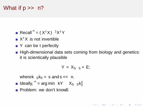
What if p >> n?

Recall β = (X tX )−1X tY

X tX is not invertible

Y can be fit perfectly

High-dimensional data sets coming from biology and genetics:it is scientifically plausible

Y = XSβS + E ,

where ‖βS‖0 = s and s << n.

Ideally, β = arg minβ ‖Y − XSβS‖22

Problem: we don’t know S

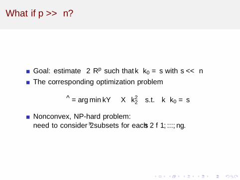
What if p >> n?

Goal: estimate β ∈ Rp such that ‖β‖0 = s with s << n

The corresponding optimization problem

β = arg minβ‖Y − Xβ‖2

2 s.t. ‖β‖0 = s

Nonconvex, NP-hard problem:need to consider 2s subsets for each s ∈ 1, ..., n.

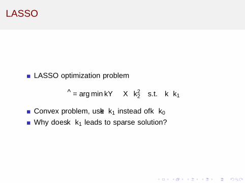
LASSO

LASSO optimization problem

β = arg minβ‖Y − Xβ‖2

2 s.t. ‖β‖1 ≤ τ

Convex problem, use ‖β‖1 instead of ‖β‖0

Why does ‖β‖1 leads to sparse solution?

Geometric intuition

Recall ordinary LSE

Geometric intuition

LSE with constraint ‖β‖1 ≤ t

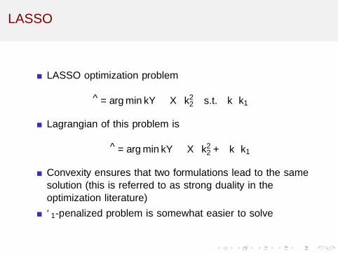
LASSO

LASSO optimization problem

β = arg minβ‖Y − Xβ‖2

2 s.t. ‖β‖1 ≤ τ

Lagrangian of this problem is

β = arg minβ‖Y − Xβ‖2

2 + λ‖β‖1

Convexity ensures that two formulations lead to the samesolution (this is referred to as strong duality in theoptimization literature)

`1-penalized problem is somewhat easier to solve

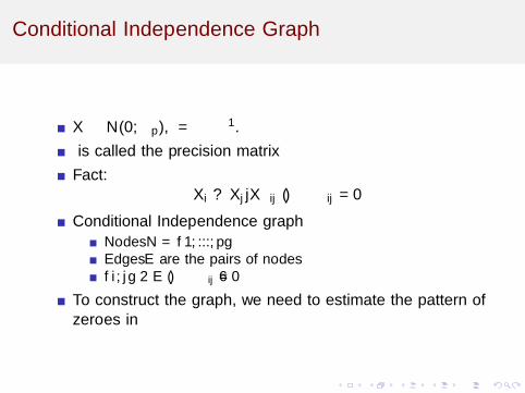
Conditional Independence Graph

X ∼ N(0,Σp), Ω = Σ−1.

Ω is called the precision matrix

Fact:Xi ⊥ Xj |X−ij ⇐⇒ Ωij = 0

Conditional Independence graph

Nodes N = 1, ..., pEdges E are the pairs of nodesi , j ∈ E ⇐⇒ Ωij 6= 0

To construct the graph, we need to estimate the pattern ofzeroes in Ω

What if p >> n?

Sample estimator of Ω:(

1nX

tX)−1

Problem 1: X tX is not invertible when p >> n

Problem 2: even if X tX is invertible, it’s unlikely that(X tX )−1 has exact zeroes

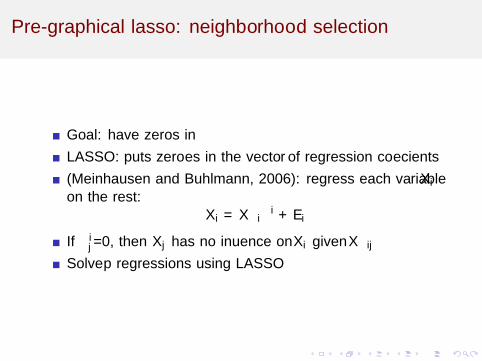
Pre-graphical lasso: neighborhood selection

Goal: have zeros in Ω

LASSO: puts zeroes in the vector β of regression coefficients

(Meinhausen and Buhlmann, 2006): regress each variable Xi

on the rest:Xi = X−iβ

i + Ei

If βij=0, then Xj has no influence on Xi given X−ij

Solve p regressions using LASSO

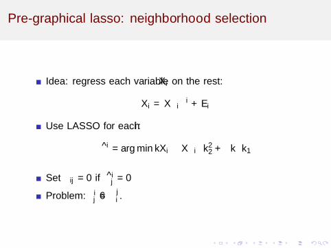
Pre-graphical lasso: neighborhood selection

Idea: regress each variable Xi on the rest:

Xi = X−iβi + Ei

Use LASSO for each i :

βi = arg minβ‖Xi − X−iβ‖2

2 + λ‖β‖1

Set Ωij = 0 if βij = 0

Problem: βij 6= βji .

Penalized Log-Likelihood

Consider the MLE, S = 1nX

tX

Ω = arg maxΘlog det Θ− Tr(SΘ).

Ω = S−1, does not serve our purpose when p >> n

Consider `1-penalized criterion

Ω = arg maxΘlog det Θ− Tr(SΘ) + λ‖Θ‖1

Here ‖Θ‖1 =∑

i

∑j |Θij |

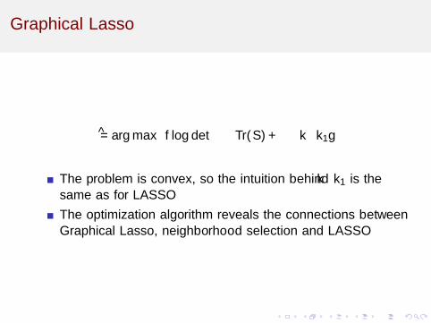
Graphical Lasso

Ω = arg maxΘlog det Θ− Tr(SΘ) + λ‖Θ‖1

The problem is convex, so the intuition behind ‖Θ‖1 is thesame as for LASSO

The optimization algorithm reveals the connections betweenGraphical Lasso, neighborhood selection and LASSO

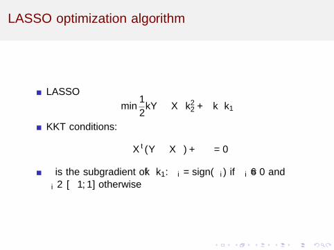
LASSO optimization algorithm

LASSO

min1

2‖Y − Xβ‖2

2 + λ‖β‖1

KKT conditions:

−X t(Y − Xβ) + λν = 0

ν is the subgradient of ‖β‖1: νi = sign(βi ) if βi 6= 0 andνi ∈ [−1, 1] otherwise

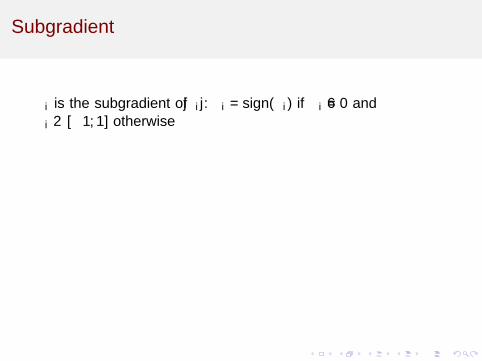
Subgradient

νi is the subgradient of |βi |: νi = sign(βi ) if βi 6= 0 andνi ∈ [−1, 1] otherwise

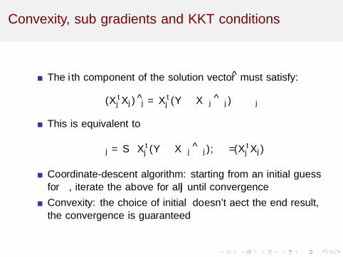
Convexity, sub gradients and KKT conditions

The ith component of the solution vector β must satisfy:

(X tj Xj)βj = X t

j (Y − X−j β−j)− λνj

This is equivalent to

βj = S(X tj (Y − X−j β−j), λ

)/(X t

j Xj)

Coordinate-descent algorithm: starting from an initial guessfor β, iterate the above for all j until convergence

Convexity: the choice of initial β doesn’t affect the end result,the convergence is guaranteed

Graphical LASSO optimization algorithm

Graphical LASSO

maxΘlog det Θ− Tr(SΘ) + λ‖Θ‖1

KKT conditions:Θ−1 − S + λΓ = 0

Γij is the subgradient of |Θij |: Γij = sign(Θij) if Θij 6= 0 andΓij ∈ [−1, 1] otherwise

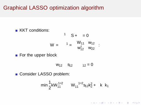
Graphical LASSO optimization algorithm

KKT conditions:Θ−1 − S + λΓ = 0

W = Θ−1 =

(W11 w12

w t12 w22

).

For the upper block

w12 − s12 − λγ12 = 0

Consider LASSO problem:

minβ

1

2‖W 1/2

11 β −W−1/211 s12‖2

2 + λ‖β‖1

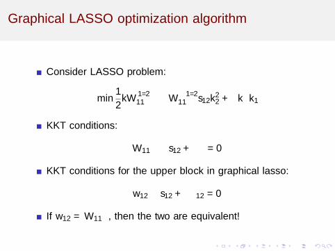
Graphical LASSO optimization algorithm

Consider LASSO problem:

minβ

1

2‖W 1/2

11 β −W−1/211 s12‖2

2 + λ‖β‖1

KKT conditions:

W11β − s12 + λν = 0

KKT conditions for the upper block in graphical lasso:

w12 − s12 + λγ12 = 0

If w12 = W11β, then the two are equivalent!

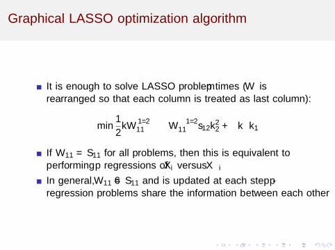
Graphical LASSO optimization algorithm

It is enough to solve LASSO problem p times (W isrearranged so that each column is treated as last column):

minβ

1

2‖W 1/2

11 β −W−1/211 s12‖2

2 + λ‖β‖1

If W11 = S11 for all problems, then this is equivalent toperforming p regressions of Xi versus X−i

In general, W11 6= S11 and is updated at each step - pregression problems share the information between each other

Conclusions

λ‖β‖1 penalty is motivated by the constraint on ‖β‖1, whichleads to zeros in β

Conclusions

Coordinate-descent methods: optimize over one variable at atime

Convexity of the problems ensure the convergence ofoptimization algorithms

KKT conditions help to draw the connections betweendifferent types of problem

Many convex problems with `1-penalty can be viewed as aspecial type of LASSO regression problem (graphical lasso,discriminant analysis, etc.)