Lasso adjustments of treatment effect estimates inrandomized experiments

Adam Bloniarz∗ Hanzhong Liu† Cun-Hui Zhang‡ Jasjeet Sekhon§

Bin Yu¶

December 20, 2015

AbstractWe provide a principled way for investigators to analyze random-ized experiments when the number of covariates is large. Investiga-tors often use linear multivariate regression to analyze randomizedexperiments instead of simply reporting the difference of means be-tween treatment and control groups. Their aim is to reduce the vari-ance of the estimated treatment effect by adjusting for covariates.If there are a large number of covariates relative to the number ofobservations, regression may perform poorly because of overfitting.In such cases, the Lasso may be helpful. We study the resultingLasso-based treatment effect estimator under the Neyman-Rubinmodel of randomized experiments. We present theoretical condi-tions that guarantee that the estimator is more efficient than thesimple difference-of-means estimator, and we provide a conserva-tive estimator of the asymptotic variance, which can yield tighterconfidence intervals than the difference-of-means estimator. Sim-ulation and data examples show that Lasso-based adjustment canbe advantageous even when the number of covariates is less thanthe number of observations. Specifically, a variant using Lasso forselection and OLS for estimation performs particularly well, and itchooses a smoothing parameter based on combined performance ofLasso and OLS.

Keywords

Randomized experiment, Neyman-Rubin model, average treatment

effect, high-dimensional statistics, Lasso, concentration inequality

1. Introduction

Randomized experiments are widely used to measure theefficacy of treatments. Randomization ensures that treat-ment assignment is not influenced by any potential con-founding factors, both observed and unobserved. Exper-iments are particularly useful when there is no rigoroustheory of a system’s dynamics, and full identification ofconfounders would be impossible. This advantage was

∗Department of Statistics, University of California, Berkeley, CA.†Department of Statistics, University of California, Berkeley, CA.‡Department of Statistics and Biostatistics, Rutgers University,

Piscataway, NJ§Department of Political Science, Department of Statistics, Uni-

versity of California, Berkeley, CA¶Department of Statistics, Department of Electrical Engineering

and Computer Science, University of California, Berkeley, CA

cast elegantly in mathematical terms in the early 20thcentury by Jerzy Neyman, who introduced a simple modelfor randomized experiments, which showed that the dif-ference of average outcomes in the treatment and controlgroups is statistically unbiased for the Average TreatmentEffect (ATE) over the experimental sample [1].

However, no experiment occurs in a vacuum of scien-tific knowledge. Often, baseline covariate informationis collected about individuals in an experiment. Evenwhen treatment assignment is not related to these covari-ates, analyses of experimental outcomes often take theminto account with the goal of improving the accuracy oftreatment effect estimates. In modern randomized ex-periments, the number of covariates can be very large—sometimes even larger than the number of individuals inthe study. In clinical trials overseen by regulatory bod-ies like the FDA and MHRA, demographic and geneticinformation may be recorded about each patient. In ap-plications in the tech industry, where randomization isoften called A/B testing, there is often a huge amount ofbehavioral data collected on each user. However, in this‘big data’ setting, much of this data may be irrelevant tothe outcome being studied or there may be more potentialcovariates than observations, especially once interactionsare taken into account. In these cases, selection of impor-tant covariates or some form of regularization is necessaryfor effective regression adjustment.

To ground our discussion, we examine a randomizedtrial of the Pulmonary Artery Catheter (PAC) that wascarried out in 65 intensive care units in the UK between2001 and 2004, called PAC-man [2]. The PAC is a moni-toring device commonly inserted into critically ill patientsafter admission to intensive care, and it provides a contin-uous measurement of several indicators of cardiac activ-ity. However, insertion of PAC is an invasive procedurethat carries some risk of complications (including death),and it involves significant expenditure both in equipmentcosts and personnel [3]. Controversy over its use came toa head when an observational study found that PAC had

1

an adverse effect on patient survival and led to increasedcost of care [4]. This led to several large-scale randomizedtrials, including PAC-man.

In the PAC-man trial, randomization of treatment waslargely successful, and a number of covariates were mea-sured about each patient in the study. If covariate inter-actions are included, the number of covariates exceeds thenumber of individuals in the study; however, few of themare predictive of the patient’s outcome. As it turned out,the (pre-treatment) estimated probability of death wasimbalanced between the treatment and control groups (p= 0.005, Wilcoxon rank sum test). Because the controlgroup had, on average, a slightly higher risk of death,the unadjusted difference-in-means estimator may over-estimate the benefits of receiving a PAC. Adjustment forthis imbalance seems advantageous in this case, since thepre-treatment probability of death is clearly predictive ofhealth outcomes post-treatment.

In this paper, we study regression-based adjustment,using the Lasso to select relevant covariates. Standardlinear regression based on ordinary least squares suffersfrom over-fitting if a large number of covariates and in-teraction terms are included in the model. In such cases,researchers sometimes perform model selection based onobserving which covariates are unbalanced given the real-ized randomization. This generally leads to misleading in-ferences because of incorrect test levels [5]. The Lasso [6]provides researchers with an alternative that can mitigatethese problems and still perform model selection. We de-

fine an estimator, ATELasso, which is based on runningan l1-penalized linear regression of the outcome on treat-ment, covariates and, following the method introducedin [7], treatment × covariate interactions. Because ofthe geometry of the l1 penalty, the Lasso will usually setmany regression coefficients to 0, and is well defined evenif the number of covariates is larger than the number ofobservations. The Lasso’s theoretical properties underthe standard linear model have been widely studied inthe last decade; consistency properties for coefficient es-timation, model selection, and out-of-sample predictionare well understood (see [8] for an overview).

In the theoretical analysis in this paper, instead ofassuming that the standard linear model is the truedata-generating mechanism, we work under the afore-mentioned non-parametric model of randomization intro-duced by Neyman [1] and popularized by Donald Ru-bin [9]. In this model, the outcomes and covariates arefixed quantities, and the treatment group is assumed tobe sampled without replacement from a finite population.The treatment indicator, rather than an error term, isthe source of randomness, and it determines which of twopotential outcomes is revealed to the experimenter. Un-like the standard linear model, the Neyman-Rubin modelmakes few assumptions not guaranteed by the random-

ization itself. The setup of the model does rely on thestable unit treatment value assumption (SUTVA), whichstates that there is only one version of treatment, and thatthe potential outcome of one unit should be unaffectedby the particular assignment of treatments to the otherunits; however it makes no assumptions of linearity or ex-ogeneity of error terms. Ordinary Least Squares (OLS)[10][11][7], logistic regression [12], and post-stratification[13] are among the adjustment methods that have beenstudied under this model.

To be useful to practitioners, the Lasso-based treat-ment effect estimator must be consistent and yield amethod to construct valid confidence intervals. We out-line conditions on the covariates and potential outcomesthat will guarantee these properties. We show that an up-per bound for the asymptotic variance can be estimatedfrom the model residuals, yielding asymptotically con-servative confidence intervals for the average treatmenteffect which can be substantially narrower than the un-adjusted confidence intervals. Simulation studies are pro-vided to show the advantage of the Lasso adjusted esti-mator and to show situations where it breaks down. Weapply the estimator to the PAC-man data, and comparethe estimates and confidence intervals derived from theunadjusted, OLS-adjusted, and Lasso-adjusted methods.We also compare different methods of selecting the Lassotuning parameter on this data.

2. Framework and definitions

We give a brief outline of the Neyman-Rubin model fora randomized experiment; the reader is urged to consult[1], [9], and [14] for more details. We follow the notationintroduced in [10] and [7]. For concreteness, we illustratethe model in the context of the PAC-man trial.

For each individual in the study, the model assumesthat there exists a pair of quantities representing his/herhealth outcomes under the possibilities of receiving andnot receiving the catheter. These are called the potentialoutcomes under treatment and control, and are denotedas ai and bi, respectively. In the course of the study,the experimenter observes only one of these quantitiesfor each individual, since the catheter is either insertedor not. The causal effect of the treatment on individual iis defined, in theory, to be ai−bi, but this is unobservable.Instead of trying to infer individual-level effects, we willassume that the intention is to estimate the average causaleffect over the whole population, as outlined in the nextsection.

In the mathematical specification of this model we con-sider the potential outcomes to be fixed, non-randomquantities, even though they are not all observable. Theonly randomness in the model comes from the assignment

2

of treatment, which is controlled by the experimenter. Wedefine random treatment indicators Ti, which take on avalue 1 for a treated individual, or 0 for an untreated indi-vidual. We will assume that the set of treated individualsis sampled without replacement from the full population,where the size of the treatment group is fixed beforehand;thus the Ti are identically distributed but not indepen-dent. The model for the observed outcome for individuali, defined as Yi, is thus

Yi = Tiai + (1− Ti)bi.

This equation simply formalizes the idea that the exper-imenter observes the potential outcome under treatmentfor those who receive the treatment, and the potentialoutcome under control for those who do not.

Note that the model does not incorporate any covari-ate information about the individuals in the study, suchas physiological characteristics or health history. How-ever, we will assume we have measured a vector of base-line, pre-experimental covariates for each individual i.These might include, for example, age, gender, and ge-netic makeup. We denote the covariates for individuali as the column vector xi = (xi1, ..., xip)

T ∈ Rp and thefull design matrix of the experiment as X = (x1, ...,xn)T .In the theoretical results, we will assume that there is acorrelational relationship between an individual’s poten-tial outcomes and covariates, but we will not assume agenerative statistical model.

Define the set of treated individuals as A = {i ∈{1, ..., n} : Ti = 1}, and similarly define the set of controlindividuals as B. Define the number of treated and con-trol individuals as nA = |A| and nB = |B|, respectively,so that nA + nB = n. To indicate averages of quantitiesover these individuals, we introduce the notation ·A and·B . Thus, for example, the average value of the potentialoutcomes and the covariates in the treatment group are

aA = n−1A∑i∈Aai, xA = n−1A

∑i∈Axi,

respectively. Note that these are random quantities inthis model, since the set A is determined by the randomtreatment assignment. When we want to take the averageover the whole population, we will use the notation ·, suchas

a = n−1∑ni=1ai, b = n−1

∑ni=1bi, x = n−1

∑ni=1xi.

Note that the averages of potential outcomes over thewhole population are not considered random, but are un-observable.

3. Treatment effect estimation

Our main inferential goal will be average effect of thetreatment over the whole population in the study. In

a trial such as PAC-man, this represents the differencebetween the average outcome if everyone had received thecatheter, and the average outcome if no one had receivedit. This is defined as

ATE = a− b.

The most natural estimator arises by replacing the pop-ulation averages with the sample averages:

ATEunadjdef= aA − bB ,

The subscript “unadj” indicates an estimator without re-gression adjustment. The foundational work in [1] pointsout that, under a randomized assignment of treatment,

ATEunadj is unbiased for ATE, and derives a conserva-tive procedure for estimating its variance.

While ATEunadj is an attractive estimator, covariateinformation can be used to make adjustments in the hopeof reducing variance. A commonly used estimator is

ATEadj =[aA − (xA − x)

Tβ(a)]−[bB − (xB − x)

Tβ(b)]

where β(a), β

(b)∈ Rp are adjustment vectors for the

treatment and control groups, respectively, as indicatedby the superscripts. The terms xA − x and xB − x rep-resent the fluctuation of the covariates in the subsamplerelative to the full sample, and the adjustment vectors fitthe linear relationships between the covariates and poten-tial outcomes under treatment and control. For example,in the PAC-man trial, this would help alleviate the imbal-ance in the pre-treatment estimated probability of death:the corresponding element of xB − x would be positive(due to the higher average probability of death in the

control group), the corresponding element of β(b)

wouldbe negative (a higher probability of death correlates withworse health outcomes), so the overall treatment effectestimate would be adjusted downwards. This procedureis equivalent to imputing the unobserved potential out-comes; if we define

ˆaB = aA + (xB − xA)Tβ(a), ˆbA = bB + (xA − xB)

Tβ(b),

we can form the equivalent estimator

ATEadj = n−1(nAaA + nB ˆaB

)− n−1

(nB bB + nA

ˆbA

).

If we consider these adjustment vectors to be fixed (non-random), or if they are derived from an independent datasource, then this estimator is still unbiased, and mayhave substantially smaller asymptotic and finite-samplevariance than the unadjusted estimator. This allows forconstruction of tighter confidence intervals for the truetreatment effect.

3

In practice, the “ideal” linear adjustment vectors, lead-ing to a minimum-variance estimator of the form of

ATEadj, cannot be computed from the observed data.However, they can be estimated, possibly at the expenseof introducing modest finite-sample bias into the treat-ment effect estimate. In the classical setup, when thenumber of covariates is relatively small, ordinary leastsquares (OLS) regression can be used. The asymptoticproperties of this kind of estimator are explored underthe Neyman-Rubin model in [11], [12], and [7]. We willfollow a particular scheme which is studied in [7] andshown to have favorable properties: we regress the out-come on treatment indicators, covariates, and treatment× covariate interactions. This is equivalent to runningseparate regressions in the treatment and control groupsof outcome against an intercept and covariates. If we de-

fine β(a)

OLS and β(b)

OLS as the coefficients from the separateregressions, then the estimator is

ATEOLS =[aA − (xA − x)

Tβ(a)

OLS

]−[bB − (xB − x)

Tβ(b)

OLS

].

This has some finite-sample bias, but [7] shows that itvanishes quickly at the rate of 1/n under moment condi-tions on the potential outcomes and covariates. Moreover,for a fixed p, under regularity conditions, the inclusionof interaction terms guarantees that it never has higherasymptotic variance than the unadjusted estimator, andasymptotically conservative confidence intervals for thetrue parameter can be constructed.

In modern randomized trials, where a large numberof covariates are recorded for each individual, p may becomparable to or even larger than n. In this case OLSregression can overfit the data badly, or may even be ill-posed, leading to estimators with large finite-sample vari-ance. To remedy this, we propose estimating the adjust-ment vectors using the Lasso [6]. The adjustment vectorswould take the form

β(a)

Lasso = arg minβ

[1

2nA

∑i∈A

(ai − aA − (xi − xA)Tβ

)2+λa

p∑j=1

|βj |],

(1)

β(b)

Lasso = arg minβ

[1

2nB

∑i∈B

(bi − bB − (xi − xB)Tβ

)2+λb

p∑j=1

|βj |],

(2)

and the proposed Lasso adjusted ATE estimator is1

ATELasso =[aA − (xA − x)

Tβ(a)

Lasso

]−[bB − (xB − x)

Tβ(b)

Lasso

].

Here λa and λb are regularization parameters for theLasso which must be chosen by the experimenter; sim-ulations show that cross-validation works well. In thenext section, we study this estimator under the Neyman-Rubin model, and provide conditions on the potentialoutcomes, the covariates and the regularization parame-

ters under which ATELasso enjoys similar asymptotic and

finite-sample advantages as ATEOLS.

It is worth noting that when two different adjustmentsare made for the treatment and control groups as in [7]and here, the covariates do not have to be the same forthe two groups. However, when they are not the same,the Lasso or OLS adjusted estimators are no longer guar-anteed to have smaller or equal asymptotic variance thanthe unadjusted one, even in the case of fixed p. In prac-tice, one may still choose between the adjusted and unad-justed estimators based on the widths of the correspond-ing confidence intervals.

4. Theoretical results

4.1. Notation

For a vector β ∈ Rp and a subset S ⊂ {1, ..., p}, let βj bethe j-th component of β, βS = (βj : j ∈ S)T , Sc be thecomplement of S, and |S| the cardinality of the set S. Forany column vector u = (u1, ..., um)T , let ‖u‖22 =

∑mi=1 u

2i ,

‖u‖1 =∑mi=1 |ui|, ‖u‖∞ = maxi=1,...,m |ui| and ‖u‖0 =

|{j : uj 6= 0}|. For a given m×m matrix D, let λmin(D)and λmax(D) be the smallest and largest eigenvalues ofD respectively, and D−1 the inverse of the matrix D.

Letd→ and

p→ denote convergence in distribution and inprobability, respectively.

4.2. Decomposition of the potentialoutcomes

The Neyman-Rubin model does not assume a linearrelationship between the potential outcomes and the co-variates. In order to study the properties of adjustmentunder this model, we decompose the potential outcomesinto a term linear in the covariates and an error term.

1To simplify the notation, we omit the dependence of β(a)Lasso,

β(b)Lasso, λa and λb on the population size n.

4

Given vectors of coefficients β(a),β(b) ∈ Rp, we write2 fori = 1, ..., n,

ai = a+ (xi − x)Tβ(a) + e(a)i , (3)

bi = b+ (xi − x)Tβ(b) + e(b)i . (4)

Note that we have not added any assumptions to the

model; we have simply defined unit-level residuals, e(a)i

and e(b)i , given the vectors β(a),β(b). All the quantities

in 3 and 4 are fixed, deterministic numbers. It is easy toverify that e(a) = e(b) = 0. In order to pursue a theoryfor the Lasso, we will add assumptions on the populationsof ai’s, bi’s, and xi’s, and we will assume the existenceof β(a),β(b) such that the error terms satisfy certain as-sumptions.

4.3. Conditions

We will need the following to hold for both the treatmentand control potential outcomes. The first set of assump-tions (1-3) are similar to those found in [7].

Condition 1 Stability of treatment assignment probabil-ity.

nA/n→ pA, as n→∞ (5)

for some pA ∈ (0, 1).

Condition 2 The centered moment conditions. Thereexists a fixed constant L > 0 such that, for all n = 1, 2, ...and j = 1, ..., p,

n−1∑ni=1 (xij − (x)j)

4 ≤ L; (6)

n−1∑ni=1(e

(a)i )4 ≤ L; n−1

∑ni=1(e

(b)i )4 ≤ L. (7)

Condition 3 The means n−1∑ni=1(e

(a)i )2, n−1

∑ni=1(e

(b)i )2

and n−1∑ni=1e

(a)i e

(b)i converge to finite limits.

Since we consider the high-dimensional setting where pis allowed to be much larger than n, we need additionalassumptions to ensure that the Lasso is consistent forestimating β(a) and β(b). Before stating them, we defineseveral quantities.

Def inition 1 Given β(a) and β(b), the sparsity measuresfor treatment and control groups, s(a) and s(b), are definedas the number of nonzero elements of β(a) and β(b), i.e.,

s(a) = |{j : β(a)j 6= 0}|, s(b) = |{j : β

(b)j 6= 0}|, (8)

respectively. We will allow s(a) and s(b) to grow with n,though the notation does not explicitly show this.

2Again, we omit the dependence of β(a), β(b), λa, λb, e(a) and

e(b) on n.

Def inition 2 Define δn to be the maximum covariancebetween the error terms and the covariates.

δn = maxω=a,b

{maxj

∣∣∣∣∣ 1nn∑i=1

(xij − (x)j)(e(ω)i − e(ω)

)∣∣∣∣∣}. (9)

The following conditions will guarantee that the Lassoconsistently estimates the adjustment vectors β(a),β(b)

at a fast enough rate to ensure asymptotic normality of

ATELasso. It is an open question whether a weaker formof consistency would be sufficient for our results to hold.

Condition 4 Decay and scaling. Let s = max{s(a), s(b)

}.

δn = o

(1

s√

log p

). (10)

(s log p)/√n = o(1). (11)

Condition 5 Cone invertibility factor. Define the Grammatrix as Σ = n−1

∑ni=1(xi − x)(xi − x)T : There exist

constants C > 0 and ξ > 1 not depending on n, such that

‖hS‖1 ≤ Cs‖Σh‖∞, ∀h ∈ C, (12)

with C = {h : ‖hSc‖1 ≤ ξ‖hS‖1}, and

S = {j : β(a)j 6= 0 or β

(b)j 6= 0}. (13)

Condition 6 Let τ = min{

1/70, (3pA)2/70, (3 −3pA)2/70

}. For constants 0 < η < ξ−1

ξ+1 and 1η < M <∞,

assume the regularization parameters of the Lasso belongto the sets

λa ∈ (1

η,M ]×

(2(1 + τ)L1/2

pA

√2 log p

n+ δn

), (14)

λb ∈ (1

η,M ]×

(2(1 + τ)L1/2

pB

√2 log p

n+ δn

). (15)

Denote respectively the population variances of e(a)

and e(b) and the population covariance between them by

σ2e(a) = n−1

∑ni=1(e

(a)i )2, σ2

e(b) = n−1∑ni=1(e

(b)i )2,

σe(a)e(b) = n−1∑ni=1e

(a)i e

(b)i .

Theorem 1 Assume conditions 1 through 6 hold forsome β(a) and β(b). Then

√n(ATELasso −ATE

)d→ N

(0, σ2

)(16)

where

σ2 = limn→∞

[1− pApA

σ2e(a) +

pA1− pA

σ2e(b) + 2σe(a)e(b)

].

(17)

5

The proof of Theorem 1 is given in the supporting in-formation. It is easy to show, as in the following corollary

of Theorem 1, that the asymptotic variance of ATELasso

is no worse than ATEunadj when β(a) and β(b) are de-fined as coefficients of regressing potential outcomes ona subset of covariates. More specifically, suppose thereexists a subset J ⊂ {1, ..., p}, such that

β(a) = ((β(a)J )T ,0)T , β(b) = ((β

(b)J )T ,0)T , (18)

where β(a)J and β

(b)J are the population level OLS coef-

ficients for regressing the potential outcomes a and b onthe covariates in the subset J with intercept, respectively.

Corollary 1 For β(a) and β(b) defined in 18 and someλa and λb, assume conditions 1 through 6 hold. Then the

asymptotic variance of√n ATELasso is no greater than

that of the√n ATEunadj. The difference is 1

pA(1−pA)∆,

where

∆ = − limn→∞

‖XβE‖22 ≤ 0, (19)

βE = (1− pA)β(a) + pAβ(b). (20)

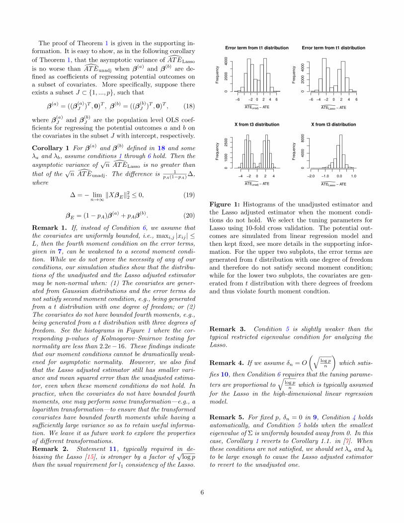
Remark 1. If, instead of Condition 6, we assume thatthe covariates are uniformly bounded, i.e., maxi,j |xij | ≤L, then the fourth moment condition on the error terms,given in 7, can be weakened to a second moment condi-tion. While we do not prove the necessity of any of ourconditions, our simulation studies show that the distribu-tions of the unadjusted and the Lasso adjusted estimatormay be non-normal when: (1) The covariates are gener-ated from Gaussian distributions and the error terms donot satisfy second moment condition, e.g., being generatedfrom a t distribution with one degree of freedom; or (2)The covariates do not have bounded fourth moments, e.g.,being generated from a t distribution with three degrees offreedom. See the histograms in Figure 1 where the cor-responding p-values of Kolmogorov–Smirnov testing fornormality are less than 2.2e−16. These findings indicatethat our moment conditions cannot be dramatically weak-ened for asymptotic normality. However, we also findthat the Lasso adjusted estimator still has smaller vari-ance and mean squared error than the unadjusted estima-tor, even when these moment conditions do not hold. Inpractice, when the covariates do not have bounded fourthmoments, one may perform some transformation—e.g., alogarithm transformation—to ensure that the transformedcovariates have bounded fourth moments while having asufficiently large variance so as to retain useful informa-tion. We leave it as future work to explore the propertiesof different transformations.Remark 2. Statement 11, typically required in de-biasing the Lasso [15], is stronger by a factor of

√log p

than the usual requirement for l1 consistency of the Lasso.

Error term from t1 distribution

ATEunadj − ATE

Fre

quency

−6 −2 0 2 4 6

02000

4000

Error term from t1 distribution

ATELasso − ATE

Fre

quency

−6 −4 −2 0 2 4 6

02000

4000

X from t3 distribution

ATEunadj − ATE

Fre

quency

−4 −2 0 2 4

01000

2500

X from t3 distribution

ATELasso − ATE

Fre

quency

−2.0 −1.0 0.0 1.0

04000

8000

Figure 1: Histograms of the unadjusted estimator andthe Lasso adjusted estimator when the moment condi-tions do not hold. We select the tuning parameters forLasso using 10-fold cross validation. The potential out-comes are simulated from linear regression model andthen kept fixed, see more details in the supporting infor-mation. For the upper two subplots, the error terms aregenerated from t distribution with one degree of freedomand therefore do not satisfy second moment condition;while for the lower two subplots, the covariates are gen-erated from t distribution with there degrees of freedomand thus violate fourth moment condtion.

Remark 3. Condition 5 is slightly weaker than thetypical restricted eigenvalue condition for analyzing theLasso.

Remark 4. If we assume δn = O

(√log pn

)which satis-

fies 10, then Condition 6 requires that the tuning parame-

ters are proportional to√

log pn which is typically assumed

for the Lasso in the high-dimensional linear regressionmodel.

Remark 5. For fixed p, δn = 0 in 9, Condition 4 holdsautomatically, and Condition 5 holds when the smallesteigenvalue of Σ is uniformly bounded away from 0. In thiscase, Corollary 1 reverts to Corollary 1.1. in [7]. Whenthese conditions are not satisfied, we should set λa and λbto be large enough to cause the Lasso adjusted estimatorto revert to the unadjusted one.

6

5. Neyman-type conservativevariance estimate

We note that the asymptotic variance in Theorem 1 in-volves the cross-product term σe(a)e(b) which is not consis-tently estimable in the Neyman-Rubin model as ai and biare never simultaneously observed. However, we can givea Neyman-type conservative estimate of the variance. Let

σ2e(a) =

1

nA − df (a)∑i∈A

(ai − aA − (xi − xA)T β

(a)

Lasso

)2,

(21)

σ2e(b) =

1

nB − df (b)∑i∈B

(bi − bB − (xi − xB)T β

(b)

Lasso

)2,

(22)where df (a) and df (b) are degrees of freedom defined by

df (a) = s(a) + 1 = ||β(a)

Lasso||0 + 1;

df (b) = s(b) + 1 = ||β(b)

Lasso||0 + 1.

Define the variance estimate of√n(ATELasso −ATE)

as follows:

σ2Lasso =

n

nAσ2e(a) +

n

nBσ2e(b) . (23)

Condition 7 For the Gram matrix Σ defined in Condi-tion 5, the largest eigenvalue is bounded away from ∞,that is, there exists a constant Λmax <∞ such that

λmax (Σ) ≤ Λmax.

Theorem 2 Assume conditions in Theorem 1 and con-dition 7 hold. Then σ2

Lasso converges in probability to

1

pAlimn→∞

σ2e(a) +

1

1− pAlimn→∞

σ2e(b) ,

which is greater than or equal to the asymptotic variance

of√n(ATELasso −ATE). The difference is

limn→∞

1

n

n∑i=1

[ai − bi −ATE − (xi − x)T (β(a) − β(b))

]2.

Remark 6. The Neyman-type conservative variance es-timate for the unadjusted estimator is given by

σ2unadj =

n

nA

1

nA − 1

∑i∈A

(ai − aA)2+n

nB

1

nB − 1

∑i∈B

(bi − bB

)2,

which, under second moment conditions of potential out-comes a and b, converges in probability to

1

pAlimn→∞

1

n

n∑i=1

(ai − a)2 +1

1− pAlimn→∞

1

n

n∑i=1

(bi − b)2.

Therefore, for the β(a) and β(b) defined in [18], the limitof σ2

Lasso is no greater than that of σ2unadj and the differ-

ence is

− limn→∞

1

n

n∑i=1

1

pA

[(xi−x)T (β(a))

]2+

1

1− pA

[(xi−x)T (β(b))

]2.

Remark 7. With the conservative variance estimate inTheorem 2, the Lasso adjusted confidence interval is alsovalid for the PATE (Population Average Treatment Ef-fect) if there is a super population of size N with N > n.Remark 8. The extra Condition 7 is used to obtain thefollowing bounds for the number of selected covariates bythe Lasso: max (s(a), s(b)) = op(min (nA, nB)). Condi-tion 7 can be removed from Theorem 2 if we redefine σ2

e(a)

and σ2e(b)

without adjusting the degrees of freedom, i.e.,

(σ∗)2e(a) =1

nA

∑i∈A

(ai − aA − (xi − xA)T β

(a)

Lasso

)2,

(σ∗)2e(b) =1

nB

∑i∈B

(bi − bB − (xi − xB)T β

(b)

Lasso

)2,

and define (σ∗)2Lasso = nnA

(σ∗)2e(a)

+ nnB

(σ∗)2e(b)

. It follows

from the bounds for max (s(a), s(b)) that (σ2e(a)

, σ2e(b)

) and((σ∗)2

e(a), (σ∗)2

e(b)) have the same asymptotic property.

Theorem 3 Assume the conditions in Theorem 1 hold.Then (σ∗)2Lasso converges in probability to

1

pAlimn→∞

σ2e(a) +

1

1− pAlimn→∞

σ2e(b) .

Remark 9. Though (σ∗)2Lasso has the same limit asσ2Lasso, our simulation experience shows that, in finite

samples, the confidence intervals based on (σ∗)2Lasso mayyield low coverage probabilities (e.g., the coverage prob-ability for 95% confidence interval can be only 80%).Hence, we recommend readers to use σ2

Lasso in practice.

6. Related work

The Lasso has already made several appearances in theliterature on treatment effect estimation. In the con-text of observational studies, [15] constructs confidenceintervals for preconceived effects or their contrasts by de-biasing the Lasso adjusted regression, [16] employs theLasso as a formal method for selecting adjustment vari-ables via a two-stage procedure which concatenates fea-tures from models for treatment and outcome, and simi-larly, [17] gives very general results for estimating a widerange of treatment effect parameters, including the caseof instrumental variables estimation. In addition to theLasso, [18] considers nonparametric adjustments in theestimation of ATE. In works such as these, which deal

7

with observational studies, confounding is the major is-sue. With confounding, the naive difference-in-means es-timator is biased for the true treatment effect, and ad-justment is used to form an unbiased estimator. How-ever, in our work, which focuses on a randomized trial,the difference-in-means estimator is already unbiased; ad-justment reduces the variance while, in fact, introduc-ing a small amount of finite-sample bias. Another majordifference between this prior work and ours is the sam-pling framework: we operate within the Neyman-Rubinmodel with fixed potential outcomes for a finite popula-tion, where the treatment group is sampled without re-placement, while these papers assume independent sam-pling from a probability distribution with random errorterms.

Our work is related to the estimation of heterogeneousor subgroup-specific treatment effects; including interac-tion terms to allow the imputed individual-level treat-ment effects to vary according to some linear combinationof covariates. This is pursued in the high-dimensional set-ting in [19]; this work advocates solving the Lasso on areduced set of modified covariates, rather than the full setof covariate × treatment interactions, and includes exten-sions to binary outcomes and survival data. The recentwork in [20] considers the problem of designing multiple-testing procedures for detecting subgroup-specific treat-ment effects; they pose this as an optimization over test-ing procedures where constraints are added to enforceguarantees on type-I error rate and power to detect ef-fects. Again, the sampling framework in these works isdistinct from ours; they do not use the Neyman-Rubinmodel as a basis for designing the methods or investigat-ing their properties.

7. PAC data illustration andsimulations

We now return to the PAC-man study introduced earlier.We examine the data in more detail and explore the re-sults of several adjustment procedures. There were 1013patients in the PAC-man study: 506 treated (managedwith PAC) and 507 control (managed without PAC, butretaining the option of using alternative devices). Theoutcome variable is quality-adjusted life years (QALYs).One QALY represents one year of life in full health; in-hospital death corresponds to a QALY of zero. We have59 covariates about each individual in the study; we in-clude all main effects as well as 1113 two-way interactions,and form a design matrix X with 1172 columns and 1013rows. See Appendix B for more details on the designmatrix.

The assumptions that underpin the theoretical guaran-

tees of the ATELasso estimator are, in practice, not explic-

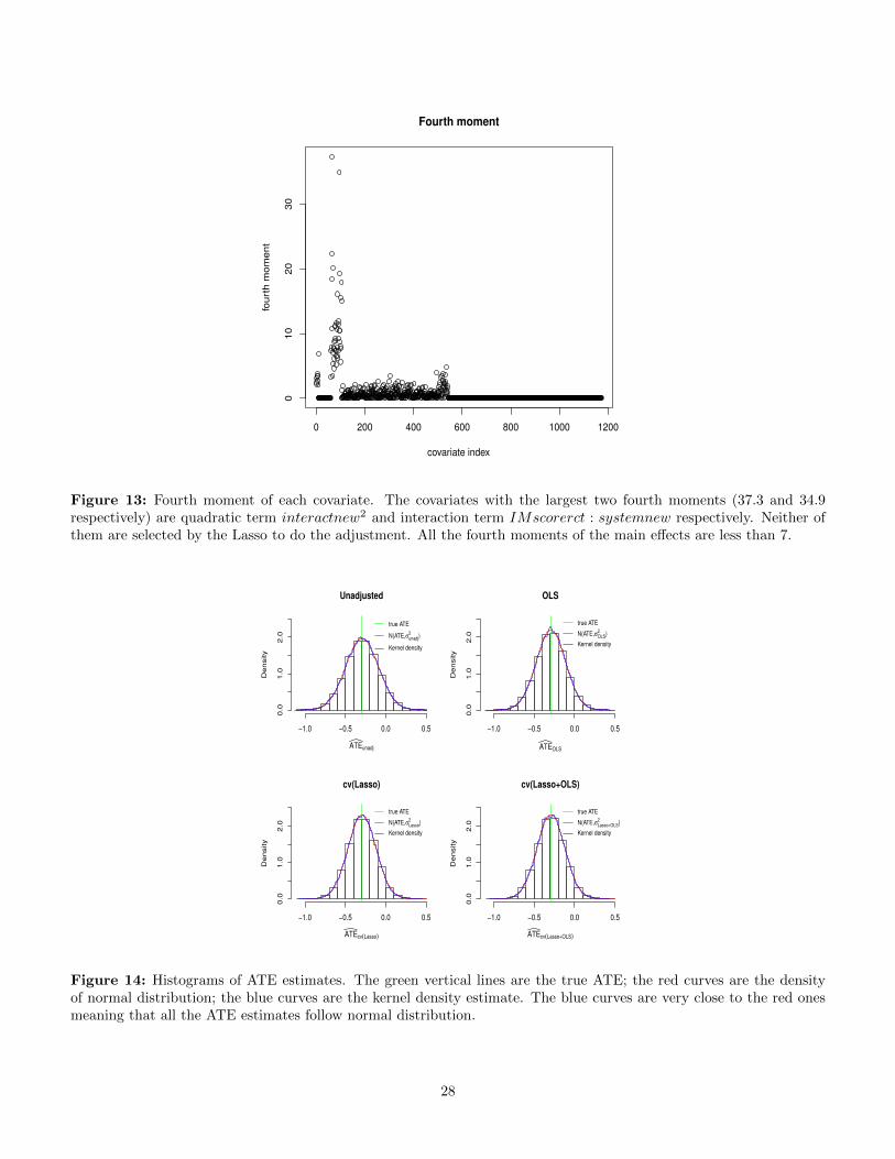
itly checkable, but we attempt to inspect the quantitiesthat are involved in the conditions to help readers maketheir own judgement. The uniform bounds on the fourthmoments refer to a hypothetical sequence of populations;these cannot be verified given that the investigator has asingle dataset. However, as an approximation, the fourthmoments of the data can be inspected to ensure that theyare not too large. In this data set, the maximum fourthmoment of the covariates is 37.3, which is indicative of aheavy-tailed and potentially destabilizing covariate; how-ever, it occurs in an interaction term not selected by thelasso, and thus does not influence the estimate3. Check-ing the conditions for high-dimensional consistency of theLasso would require knowledge of the unknown activeset S, and moreover, even if it were known, calculatingthe cone invertibility factor would involve an infeasibleoptimization. This is a general issue in the theory ofsparse linear high-dimensional estimation. To approxi-mate these conditions, we use the bootstrap to estimatethe active set of covariates S and the error terms e(a)

and e(b). See the supporting information for more details.Our estimated S contains 16 covariates and the estimatedsecond moments of e(a) and e(b) are 11.8 and 12.0, respec-tively. The estimated maximal covariance δn equals 0.34and the scaling (s log p)/

√n is 3.55. While this is not

close to zero, we should mention that the estimation of δnand (s log p)/

√n can be unstable and less accurate since

it is based on a subsample of the population. As an ap-proximation to Condition 5, we examine the largest andsmallest eigenvalues of the sub-Gram matrix (1/n)XT

SXS ,which are 2.09 and 0.18 respectively. Thus the quantityin Condition 5 seems reasonably bounded away from zero.

We now estimate the ATE using the unadjusted estima-tor, the Lasso adjusted estimator and the OLS adjustedestimator which is computed based on a sub-design ma-trix containing only the 59 main effects. We also present

results for the two-step estimator ATELasso+OLS whichadopts the Lasso to select covariates and then uses OLSto refit the regression coefficients. See [22–25] for statis-tical properties of Lasso+OLS estimator in linear regres-

sion model. Let β(a)

be the Lasso estimator defined in 1(we omit the subscript “Lasso” for the sake of simplicity)

and let S(a) = {j : β(a)

j 6= 0} be the support of β(a)

. The

Lasso+OLS adjustment vector β(a)Lasso+OLS for treatment

3The fourth moments of the covariates are shown in Fugure 13 inAppendix F. The covariates with the largest two fourth moments(37.3 and 34.9 respectively) are quadratic term interactnew2

and interaction term IMscorerct : systemnew. Neither of themare selected by the Lasso to do the adjustment.

8

group A is defined by

β(a)

Lasso+OLS = arg minβ: βj=0, ∀j /∈S(a)

1

2nA

∑i∈A

[ai − aA

−(xi − xA)Tβ]2.

We can define the Lasso+OLS adjustment vector

β(b)

Lasso+OLS for control group B similarly. Then

ATELasso+OLS is given by

ATELasso+OLS =[aA − (xA − x)T β

(a)

Lasso+OLS

]−[bB − (xB − x)T β

(b)

Lasso+OLS

].

In the next paragraph and in Algorithm 1 of AppendixF, we show how we adapt the cross-validation proce-

dure to select the tuning parameter for ATELasso+OLS

based on a combined performance of Lasso and OLS, orcv(Lasso+OLS).

We use the R package “glmnet” to compute the Lassosolution path and select the tuning parameters λa and λbby 10-fold Cross Validation (CV). To indicate the methodof selecting tuning parameters, we denote the correspond-ing estimators as cv(Lasso) and cv(Lasso+OLS) respec-tively. We should mention that for the cv(Lasso+OLS)adjusted estimator, we compute the CV error for a givenvalue of λa (or λb) based on the whole Lasso+OLS proce-dure instead of just the Lasso estimator (see Algorithm 1in Appendix F). Therefore, the cv(Lasso+OLS) and thecv(Lasso) may select different covariates to do the adjust-ment. This type of cross validation requires more compu-tation than the cross validation based on just the Lassoestimator since it needs to compute the OLS estimatorfor each fold and each given λa (or λb), but it can givebetter prediction and model selection performance.

Figure 2 presents the ATE estimates along with 95%confidence intervals (CI). The interval lengths are shownon top of each interval bar. All the methods give confi-dence intervals containing 0; hence, this experiment failedto provide sufficient evidence to reject the hypothesis thatPAC did not have an effect on patient QALYs (eitherpositive or negative). Since the caretakers of patientsmanaged without PAC retained the option of using lessinvasive cardiac output monitoring devices, such an effectmay have been particularly hard to detect in this experi-ment.

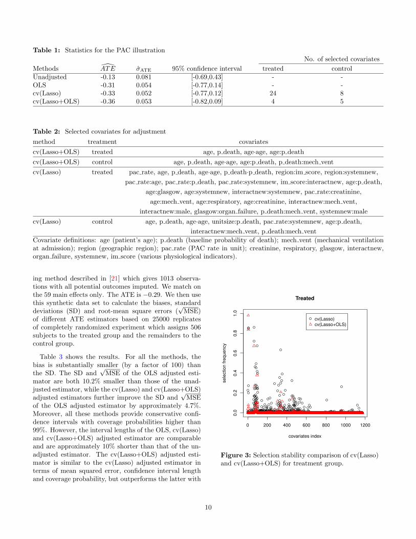
However, it is interesting to note that (see Table 1),compared with the unadjusted estimator, the OLS ad-justed estimator causes the ATE estimate to decrease(from -0.13 to -0.31), and shortens the confidence intervalby about 20%. This is due mainly to the imbalance in thepre-treatment probability of death, which was highly pre-dictive of the post-treatment QALYs. The cv(Lasso) ad-justed estimator yields a comparable ATE estimate and

−1.0

−0.5

0.0

0.5

ATE estimates for PAC data

method

AT

E e

stim

ate

s

1.11

0.91 0.9 0.9

Unadjusted OLS cv(Lasso) cv(Lasso+OLS)

Figure 2: ATE estimates (red circles) and 95% confi-dence intervals (bars) for the PAC data. The numbersabove each bar are the corresponding interval lengths.

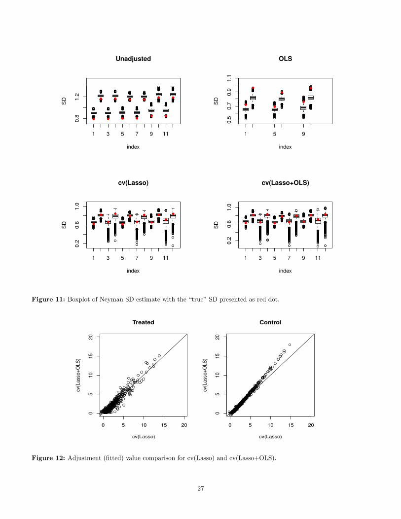
confidence interval, but the fitted model is more inter-pretable and parsimonious than the OLS model: it selects24 and 8 covariates for treated and control, respectively.The cv(Lasso+OLS) estimator selects even fewer covari-ates: 4 and 5 for treated and control, respectively, butperforms a similar adjustment as the cv(Lasso) (see thecomparison of fitted values in Figure 12). We also notethat these adjustments agree with the one performed in[13], where the treatment effect was adjusted downwardsto −0.27 after stratifying into 4 groups based on predictedprobability of death.

The covariates selected by Lasso for adjustment areshown in Table 2, where “A·A” denote quadratic termof the covariate A and “A:B” denote two way interac-tion between two covariates A and B. Among them, pa-tient’s age and estimated probability of death (p death),together with the quadratic term “age·age” and interac-tions “age:p death” and “p death:mech vent4”, are themost important covariates for the adjustment. The pa-tients in control group are slightly older and have slightlyhigher risk of death. These covariates are important pre-dictors of the outcome. Therefore, the unadjusted esti-mator may overestimate the benefits of receiving PAC.

Since not all the potential outcomes are observed, wecannot know the true gains of adjustment methods. How-ever, we can estimate the gains via building a simulatedset of potential outcomes by matching treated units tocontrol units on observed covariates. We use the match-

4mechanical ventilation at admission

9

Table 1: Statistics for the PAC illustration

No. of selected covariates

Methods ATE σATE 95% confidence interval treated controlUnadjusted -0.13 0.081 [-0.69,0.43] - -OLS -0.31 0.054 [-0.77,0.14] - -cv(Lasso) -0.33 0.052 [-0.77,0.12] 24 8cv(Lasso+OLS) -0.36 0.053 [-0.82,0.09] 4 5

Table 2: Selected covariates for adjustment

method treatment covariates

cv(Lasso+OLS) treated age, p death, age·age, age:p death

cv(Lasso+OLS) control age, p death, age·age, age:p death, p death:mech vent

cv(Lasso) treated pac rate, age, p death, age·age, p death·p death, region:im score, region:systemnew,

pac rate:age, pac rate:p death, pac rate:systemnew, im score:interactnew, age:p death,

age:glasgow, age:systemnew, interactnew:systemnew, pac rate:creatinine,

age:mech vent, age:respiratory, age:creatinine, interactnew:mech vent,

interactnew:male, glasgow:organ failure, p death:mech vent, systemnew:male

cv(Lasso) control age, p death, age·age, unitsize:p death, pac rate:systemnew, age:p death,

interactnew:mech vent, p death:mech vent

Covariate definitions: age (patient’s age); p death (baseline probability of death); mech vent (mechanical ventilationat admission); region (geographic region); pac rate (PAC rate in unit); creatinine, respiratory, glasgow, interactnew,organ failure, systemnew, im score (various physiological indicators).

ing method described in [21] which gives 1013 observa-tions with all potential outcomes imputed. We match onthe 59 main effects only. The ATE is −0.29. We then usethis synthetic data set to calculate the biases, standarddeviations (SD) and root-mean square errors (

√MSE)

of different ATE estimators based on 25000 replicatesof completely randomized experiment which assigns 506subjects to the treated group and the remainders to thecontrol group.

Table 3 shows the results. For all the methods, thebias is substantially smaller (by a factor of 100) thanthe SD. The SD and

√MSE of the OLS adjusted esti-

mator are both 10.2% smaller than those of the unad-justed estimator, while the cv(Lasso) and cv(Lasso+OLS)adjusted estimators further improve the SD and

√MSE

of the OLS adjusted estimator by approximately 4.7%.Moreover, all these methods provide conservative confi-dence intervals with coverage probabilities higher than99%. However, the interval lengths of the OLS, cv(Lasso)and cv(Lasso+OLS) adjusted estimator are comparableand are approximately 10% shorter than that of the un-adjusted estimator. The cv(Lasso+OLS) adjusted esti-mator is similar to the cv(Lasso) adjusted estimator interms of mean squared error, confidence interval lengthand coverage probability, but outperforms the latter with

0 200 400 600 800 1000 1200

0.0

0.2

0.4

0.6

0.8

1.0

Treated

covariates index

sele

ction fre

quency

cv(Lasso)

cv(Lasso+OLS)

Figure 3: Selection stability comparison of cv(Lasso)and cv(Lasso+OLS) for treatment group.

10

0 200 400 600 800 1000 1200

0.0

0.2

0.4

0.6

0.8

1.0

Control

covariates index

sele

ction fre

quency

cv(Lasso)

cv(Lasso+OLS)

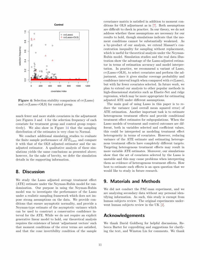
Figure 4: Selection stability comparison of cv(Lasso)and cv(Lasso+OLS) for control group.

much fewer and more stable covariates in the adjustment(see Figures 3 and 4 for the selection frequency of eachcovariate for treatment group and control group respec-tively). We also show in Figure 14 that the samplingdistribution of the estimates is very close to Normal.

We conduct additional simulation studies to evaluatethe finite sample performance of ATELasso and compareit with that of the OLS adjusted estimator and the un-adjusted estimator. A qualitative analysis of these sim-ulations yields the same conclusions as presented above;however, for the sake of brevity, we defer the simulationdetails in the supporting information.

8. Discussion

We study the Lasso adjusted average treatment effect(ATE) estimate under the Neyman-Rubin model for ran-domization. Our purpose in using the Neyman-Rubinmodel was to investigate the performance of the Lassounder a realistic sampling framework which does not im-pose strong assumptions on the data. We provide con-ditions that ensure asymptotic normality, and provide aNeyman-type estimate of the asymptotic variance whichcan be used to construct a conservative confidence in-terval for the ATE. While we do not require an explicitgenerative linear model to hold, our theoretical analysisrequires the existence of latent ‘adjustment vectors’ suchthat moment conditions of the error terms are satisfied,and that the cone invertibility condition of the sample

covariance matrix is satisfied in addition to moment con-ditions for OLS adjustment as in [7]. Both assumptionsare difficult to check in practice. In our theory, we do notaddress whether these assumptions are necessary for ourresults to hold, though simulations indicate that the mo-ment conditions cannot be substantially weakened. Asa by-product of our analysis, we extend Massart’s con-centration inequality for sampling without replacement,which is useful for theoretical analysis under the Neyman-Rubin model. Simulation studies and the real data illus-tration show the advantage of the Lasso-adjusted estima-tor in terms of estimation accuracy and model interpre-tation. In practice, we recommend a variant of Lasso,cv(Lasso+OLS), to select covariates and perform the ad-justment, since it gives similar coverage probability andconfidence interval length when compared with cv(Lasso),but with far fewer covariates selected. In future work, weplan to extend our analysis to other popular methods inhigh-dimensional statistics such as Elastic-Net and ridgeregression, which may be more appropriate for estimatingadjusted ATE under different assumptions.

The main goal of using Lasso in this paper is to re-duce the variance (and overall mean squared error) ofATE estimation. Another important task is to estimateheterogenous treatment effects and provide conditionaltreatment effect estimates for subpopulations. When theLasso models of treatment and control outcomes are dif-ferent, both in variables selected and coefficient values,this could be interpreted as modeling treatment effectheterogeneity in terms of covariates. However, reducingvariance of the ATE estimate and estimating heteroge-nous treatment effects have completely different targets.Targeting heterogenous treatment effects may result inmore variable ATE estimates. Moreover, our simulationsshow that the set of covariates selected by the Lasso isunstable and this may cause problems when interpretingthem as evidence of heterogenous treatment effects. Howbest to estimate such effects is an open question that wewould like to study in future research.

9. Materials and Methods

We did not conduct the PAC-man experiment, and weare analyzing secondary data without any personal iden-tifying information. As such, this study is exempt fromhuman subjects review. The original experiments under-went human subjects review in the UK [2].

Acknowledgements

We thank David Goldberg for helpful discussions, Re-becca Barter for copyediting and suggestions for clarify-ing the text, and Winston Lin for comments. We thank

11

Table 3: Statistics for the PAC synthetic data set

No. of selected covariates

Bias SD√

MSE Coverage (%) Length treated controlUnadjusted 0.001(0) 0.20(0.02) 0.20(0.02) 99 1.06 - -OLS 0.002(0) 0.18(0.02) 0.18(0.02) 99 0.95 - -cv(Lasso) 0.001(0) 0.17(0.02) 0.17(0.02) 99 0.94 25(23) 15(14)cv(Lasso+OLS) 0.000(0) 0.17(0.02) 0.17(0.02) 99 0.95 6(6) 4(3)The numbers in parentheses are the corresponding standard errors estimated by using the bootstrap with B = 500resamplings of the ATE estimates.

Richard Grieve (LSHTM), Sheila Harvey (LSHTM),David Harrison (ICNARC) and Kathy Rowan (IC-NARC) for access to data from the PAC-Man CEAand the ICNARC CMP database. This research is par-tially supported by NSF grants DMS-11-06753, DMS-12-09014, DMS-1107000, DMS-1129626, DMS-1209014,CDS&E-MSS, 1228246DMS-1160319 (FRG), AFOSRgrant FA9550-14-1-0016, NSA Grant H98230-15-1-0040,the Center for Science of Information (CSoI), an US NSFScience and Technology Center, under grant agreementCCF-0939370, the Department of Defense (DoD) for Of-fice of Naval Research (ONR) grant N00014-15-1-2367and the National Defense Science & Engineering Grad-uate Fellowship (NDSEG) Program.

References

[1] Splawa-Neyman J, Dabrowska DM, Speed TP (1990)On the Application of Probability Theory to Agri-cultural Experiments. Essay on Principles. Section9. Statistical Science 5(4):465–472.

[2] Harvey S et al. (2005) Assessment of the clinical ef-fectiveness of pulmonary artery catheters in man-agement of patients in intensive care (PAC-Man): arandomised controlled trial. Lancet 366(9484):472–477.

[3] Dalen JE (2001) The Pulmonary Artery Catheter —Friend, Foe, or Accomplice? Jama 286(3):348–350.

[4] Connors AF et al. (1996) The effectiveness of rightheart catheterization in the initial care of criticallyIII patients. Jama 276(11):889–897.

[5] Permutt T (1990) Testing for imbalance of covari-ates in controlled experiments. Statistics in medicine9(12):1455–1462.

[6] Tibshirani R (1994) Regression Selection and Shrink-age via the Lasso. Journal of the Royal StatisticalSociety B 58:267–288.

[7] Lin W (2013) Agnostic notes on regression adjust-ments to experimental data: reexamining Freed-man’s critique. The Annals of Applied Statistics7:295–318.

[8] Buhlmann P, Van De Geer S (2011) Statistics forhigh-dimensional data: methods, theory and applica-tions. (Springer Science & Business Media).

[9] Rubin DB (1974) Estimating causal effects of treat-ments in randomized and nonrandomized studies.Journal of Educational Psychology 66(5):688–701.

[10] Freedman DA (2008) On regression adjustments toexperimental data. Advances in Applied Mathemat-ics 40(2):180–193.

[11] Freedman DA (2008) On regression adjustments inexperiments with several treatments. The Annals ofApplied Statistics 2(1):176–196.

[12] Freedman DA (2008) Randomization does not justifylogistic regression. Statistical Science 23(2):237–249.

[13] Miratrix LW, Sekhon JS, Yu B (2013) Adjustingtreatment effect estimates by post-stratification inrandomized experiments. Journal of the Royal Sta-tistical Society. Series B: Statistical Methodology75:369–396.

[14] Holland PW (1986) Statistics and causal infer-ence. Journal of the American Statistical Association81:945–960.

[15] Zhang CH, Zhang SS (2014) Confidence intervals forlow dimensional parameters in high dimensional lin-ear models. Journal of the Royal Statistical Society:Series B (Statistical Methodology) 76(1):217–242.

[16] Belloni A, Chernozhukov V, Hansen C (2013) In-ference on Treatment Effects after Selection amongHigh-Dimensional Controls. The Review of Eco-nomic Studies 81(2):608–650.

[17] Belloni A, Chernozhukov V, Fernandez-Val I, HansenC (2013) Program evaluation with high-dimensionaldata. arXiv preprint arXiv:1311.2645.

12

[18] Li L, Tchetgen Tchetgen E, van der Vaart A, RobinsJM (2011) Higher order inference on a treatment ef-fect under low regularity conditions. Statistics &probability letters 81(7):821–828.

[19] Tian L, Alizadeh A, Gentles A, Tibshirani R (2014)A simple method for detecting interactions between atreatment and a large number of covariates. Journalof the American Statistical Association just accep.

[20] Rosenblum M, Liu H, En-Hsu Y (2014) OptimalTests of Treatment Effects for the Overall Popula-tion and Two Subpopulations in Randomized Tri-als, Using Sparse Linear Programming. Journal ofthe American Statistical Association 109(507):1216–1228.

[21] Diamond A, Sekhon JS (2013) Genetic Matching forEstimating Causal Effects: A General MultivariateMatching Method for Achieving Balance in Observa-tional Studies. Review of Economics and Statistics95(3):932–945.

[22] Meinshausen N (2007) Relaxed Lasso. Computa-tional Statistics and Data Analysis 52:374–393.

[23] Efron B, Hastie T and Tibshirani R (2004) Leastangle regression. Annals of Statistics 32:407–499.

[24] Belloni A, Chernozhukov V (2009) Least SquaresAfter Model Selection in High-dimensional SparseModels. Bernoulli 19:521-547.

[25] Liu H, Yu B (2013) Asymptotic properties ofLasso+mLS and Lasso+Ridge in sparse high-dimensional linear regression. Electronic Journal ofStatistics 7:3124–3169.

[26] Massart P (1986) in Geometrical and Statistical As-pects of Probability in Banach Spaces. (Springer),pp. 73–109.

A. Simulation

In this section we carry out simulation studies to evaluate

the finite sample performance of ATELasso estimator. We

also present results for the ATEOLS estimator when p < n

and the two-step estimator ATELasso+OLS.We use the R package “glmnet” to compute the Lasso

solution path. We select the tuning parameters λaand λb by 10-fold Cross Validation (CV) and denotethe corresponding adjusted estimators as cv(Lasso) andcv(Lasso+OLS) respectively. We should mention thatfor the cv(Lasso+OLS) adjusted estimator, we computethe CV error for a given value of the λa (or λb) based

on the whole Lasso+OLS estimator instead of the Lassoestimator, see Algorithm 1 for details. Therefore, thecv(Lasso+OLS) adjusted estimator and the cv(Lasso)adjusted estimator may select different covariates todo the adjustment. This type of cross validation forcv(Lasso+OLS) requires more computation effort thanthe cross validation based on just the Lasso estimatorsince it needs to compute the OLS estimator for each foldand for each λa (or λb), but it can give better predictionand covariates selection performance.

The potential outcomes ai and bi are generated fromthe following nonlinear model: for i = 1, ..., n,

ai =

s∑j=1

xijβ(a1)j + exp

s∑j=1

xijβ(a2)j

+ ε(a)i ,

bi =

s∑j=1

xijβ(b1)j + exp

s∑j=1

xijβ(b2)j

+ ε(b)i ,

where ε(a)i and ε

(b)i are independent error terms. We set

n = 250, s = 10, p = 50 and 500. For p = 50, we cancompute OLS estimator and compare it with the Lasso.The covariates vector xi is generated from a multivariatenormal distribution N (0,Σ). We consider two differentToeplitz covariance matrices Σ which control the correla-tion among the covariates:

Σii = 1; Σij = ρ|i−j| ∀i 6= j,

where ρ = 0, 0.6. The true coefficients β(a1)j , β

(a2)j , β

(b1)j ,

β(b2)j are generated independently according to

β(a1)j ∼ t3; β

(a2)j ∼ 0.1 ∗ t3, j = 1, ..., s,

β(b1)j ∼ β(a1)

j + t3; β(b2)j ∼ β(a2)

j + 0.1 ∗ t3, j = 1, ..., s,

where t3 denotes the t distribution with three degrees offreedom. This ensures that the treatment effects are notnot constant across individuals, and that the linear model

does not hold in this simulation. The error terms ε(a)i and

ε(b)i are generated according to the following linear model

with some hidden covariates zi:

ε(a)i =

s∑j=1

zijβ(a1)j + ε

(a)i ,

ε(b)i =

s∑j=1

zijβ(b1)j + ε

(b)i ,

where ε(a)i and ε

(b)i are drawn independently from stan-

dard normal distribution. The vector zi is independentof xi and also drawn independently from the multivari-ate normal distribution N (0,Σ). The values of xi, β

(a1),

13

β(a2), β(b1), β(b2), zi, ε(a)i , ε

(b)i , ai and bi are generated

once and then kept fixed.

After the potential outcomes are generated, a com-pletely randomized experiment is simulated 25000 times,assigning nA = 100, 125, 150 subjects to treatment A andthe remainder to control B. There are 12 different combi-nations of (p, ρ, nA) in total.

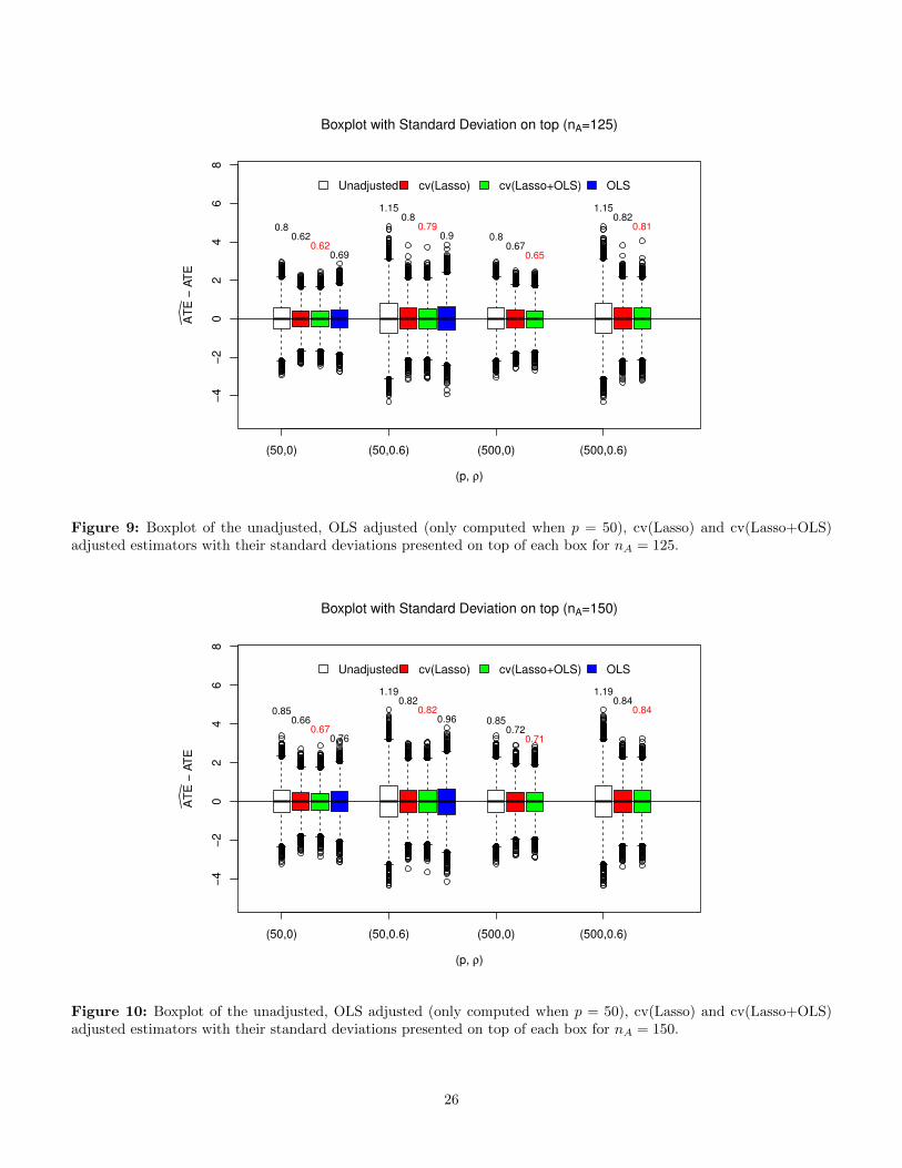
Figures 8, 9, 10 show the boxplot of different ATE es-timators with their standard deviations (computed from25000 replicates of randomized experiments) presented ontop of each box. Regardless of whether the design is bal-anced (nA = 125) or not (nA = 100, 150), the regressionbased estimators have much smaller variances and thanthat of the unadjusted estimator and therefore improvethe estimation precision.

To further compare the performance of these estima-tors, we present the bias, the standard deviation (SD)and the root-mean square error (

√MSE) of the estimates

in Table 4. Bias is reported as the absolute differencefrom the true treatment effect. We find that the bias ofeach method is substantially smaller (more than 10 timessmaller) than the SD. The cv(Lasso) and cv(Lasso+OLS)adjusted estimators perform similar in terms of SD and√

MSE: reducing those of the OLS adjusted estima-tor and the unadjusted estimator by 10% − 15% and15% − 31% respectively. We also compare the numberof selected covariates by cv(Lasso) and cv(Lasso+OLS)for treatment group and control group separately, see Ta-ble 5. It is easy to see that the cv(Lasso+OLS) adjustedestimator uses many fewer (more than 44%) covariatesin the adjustment to obtain similar improvement of SDand

√MSE of ATE estimate as the cv(Lasso) adjusted

estimator. Moreover, we find that the covariates selectedby the cv(Lasso+OLS) are more stable across differentrealizations of treatment assignment than the covariatesselected by the cv(Lasso). Overall, the cv(Lasso+OLS)adjusted, the cv(Lasso) adjusted, the OLS adjusted andthe unadjusted estimators perform from best to worst.

We move now to study the finite sample performanceof Neyman-type conservative variance estimates. Foreach simulation example and each one of the 25000 com-pletely randomized experiments, we calculate the ATE

estimates (ATE) and the Neyman variance estimates (σ)

and then form the 95% confidence intervals [ATE−1.96 ·σ/√n, ATE + 1.96 · σ/

√n]. Figures 5, 6, 7 present the

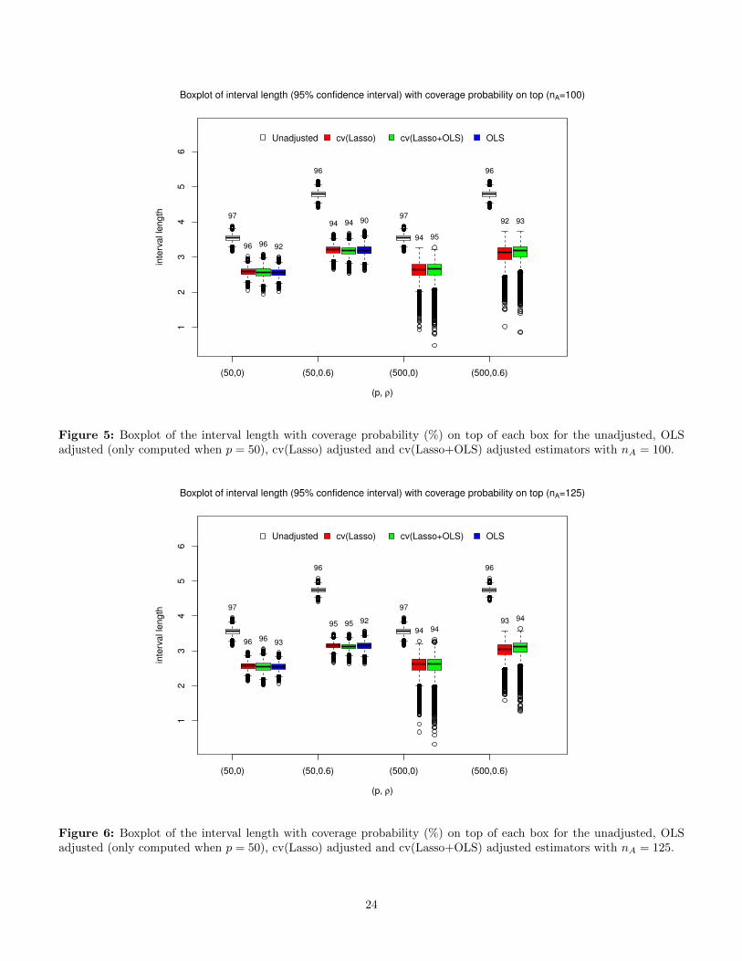
boxplot of the interval length with the coverage proba-bility noted on top of each box for the unadjusted, OLSadjusted (only computed when p = 50), cv(Lasso) ad-justed and cv(Lasso+OLS) adjusted estimators. Moreresults are showed in Table 6. We find that all the con-fidence intervals for the unadjusted estimator are conser-vative. The cv(Lasso) adjusted and the cv(Lasso+OLS0adjusted estimators perform very similar: although their

coverage probability (at least 92%) may be slightly lessthan the pre-assigned confidence level (95%), their meaninterval length is much shorter (26% − 37%) than thatof the unadjusted estimator. The OLS adjusted esti-mator has comparable interval length with the cv(Lasso)and cv(Lasso+OLS) adjusted estimator, but has slightlyworse coverage probability (90%− 93%).

To further investigate how good the Neyman standarddeviation (SD) estimate is, we compare them in Figure 11with the “true” SD presented in Table 4 (the SD of theATE estimates over 25000 randomized experiments). Wefind that Neyman SD estimate is very conservative for theunadjusted estimator (its mean is 5% − 14% larger thanthe “true” SD); while for the OLS adjusted estimator, themean of Neyman SD estimate can be 6%− 100% smallerthan the “true” SD which may be because of over-fitting.For the cv(Lasso) and cv(Lasso+OLS) adjusted estima-tor, the mean of Neyman SD estimator is within 1±7% ofthe “true” SD. Although the Neyman variance estimateis asymptotically conservative, the finite sample behaviorof the Neyman SD estimate can be progressive for theregression-based adjusted estimator. However, if we in-crease the sample size n to 1000, almost all the confidenceintervals are conservative.

We conduct more simulation examples to evaluate theconditions assumed for asymptotic normality of the Lassoadjusted estimator. We use the same simulation setup asabove, but for simplicity, we generate the potential out-comes from linear model (set β(a2) = β(b2) = 0) and re-move the effects of the hidden covariates zi in generating

the error terms ε(a)i and ε

(b)i and set ρ = 0, nA = 125.

We find that the distribution of the cv(Lasso) adjustedestimator may be non-normal when:

(1). The covariates are generated from Gaussian distri-bution and the error terms do not satisfy second mo-ment condition, e.g., being generated from t distri-bution with one degree of freedom, see the upper twosubplots of Figure 1 (in the main text) for the his-tograms of unadjusted the cv(Lasso) adjusted esti-mators (the corresponding p-values of Kolmogorov–Smirnov testing for normality are less than 2.2e−16).

(2). The covariates do not have bounded fourth moments,e.g., being generated from t distribution with threedegrees of freedom, see the lower two subplots of Fig-ure 1 (in the main text) for the histograms of unad-justed the cv(Lasso) adjusted estimators (again, thecorresponding p-values of Kolmogorov–Smirnov test-ing for normality are less than 2.2e− 16).

These findings indicate that our moment condition (Con-dition 2 and Remark 1) cannot be dramatically weak-ened. However, we also find that the cv(Lasso) adjusted

14

estimator still has smaller SD and√

MSE than the unad-justed estimator even when these moment conditions donot hold.

B. The design matrix of the PACdata

In the PAC data, there are 59 covariates (main effects)including 50 indicators which may be correlated with theoutcomes. One of the main effects (called interactnew)has heavy tail, so we do the transform: x → log(|x| + 1)to make it look like normal distributed. We then cen-tralize and standardize the non-indicator covariates. Thequadratic terms (9 in total) of non-indicator covariatesand two-way interactions between main effects (1711in total) may also contribute to predict the potentialoutcomes, so we included them in the design matrix.The quadratic terms and the interactions between non-indicator covariates and the interactions between indica-tor covariates and non-indicator covariates are also cen-tered and standardized. Some of the interactions are ex-actly the same as other effects and we only retain one ofthem. We also remove the interactions which are highlycorrelated (with correlation larger than 0.95) with themain effects and remove the indicators with very sparseentries (where the number of 1’s is less than 20). Finally,we form a design matrix X with 1172 columns (covari-ates) and 1013 rows (subjects).

C. Estimation of constants in theconditions

Let S(a) = {j : β(a)j 6= 0} and S(b) = {j : β

(b)j 6= 0}

denote the sets of relevant covariates for treatment groupand control group respectively. Denote S = S(a)

⋃S(b) =

{j : β(a)j 6= 0 or β

(b)j 6= 0}. We use bootstrap to get an

estimation of the relevant covariates sets S(a), S(b) andthen the approximation errors e(a) and e(b) are estimatedby regressing the observed potential outcomes a and b onthe covariates in S respectively. We only present how toestimate S(a) and e(a) in detail and the estimation of S(b)

and e(b) are similar.

Let A, B be the set of treated subjects (usingPAC) and control subjects (without using PAC) re-spectively. Denote ai, i ∈ A the potential outcomes(quality-adjusted life years (QALYs)) under treatmentand xi ∈ R1172 the covariates vector of the ith sub-ject. For each d = 1, ..., 1000, we draw a bootstrap sam-ple {(a∗i (d), x∗i (d)) : i ∈ A} with replacement from thedata points {(ai, xi) : i ∈ A}. Then computing the Las-

soOLS(CV) adjusted vector β(d) based on each bootstrap

sample {(a∗i (d), x∗i (d)) : i ∈ A}. Let τj be the selection

fraction of non-zero βj(d) in the 1000 bootstrap estima-

tors, i.e., τj = (1/1000)∑1000d=1 I{βj(d)6=0}, where I is the

indicator function. We form the relevant covariates S(a)

by the covariates whose selection fraction are larger than0.5: S(a) = {j : τj > 0.5}.

To estimate the approximation error e(a), we regress aion the relevant covariates xij , j ∈ S(a) and compute OLS

estimate and the corresponding residual. That is, let T (a)

denote the complement set of S(a),

β(a)OLS = arg min

β: βj=0, ∀j∈T (a)

1

2nA

∑i∈A

(ai − aA − (xi − xA)Tβ

)2.

e(a)i = ai − aA − (xi − xA)Tβ

(a)OLS, i ∈ A.

The maximal covariance δn is estimated as:

max

{maxj

∣∣∣∣∣ 1

nA

∑i∈A

(xij − (x)j)(e(a)i − e

(a)A

)∣∣∣∣∣ ,maxj

∣∣∣∣∣ 1

nB

∑i∈B

(xij − (x)j)(e(b)i − e

(b)B

)∣∣∣∣∣}.

D. Proofs of Theorem 1, 2, 3 andCorollary 1

In this section, we will prove Theorem 1 - 3 and Corollary1 under weaker sparsity conditions.

Def inition 3 We define an approximate sparsity mea-sure. Given the regularization parameter λa, λb and β(a)

and β(b), the sparsity measures for treatment and control

groups, s(a)λa

and s(b)λb

are defined as

s(a)λa

=

p∑j=1

min

{|β(a)j |λa

, 1

}, s

(b)λb

=

p∑j=1

min

{|β(b)j |λb

, 1

},

(24)

respectively. We will allow s(a)λa

and s(b)λb

to grow with n,though the notation does not explicitly show this. Notethat this is weaker than strict sparsity, as it allows β(a)

and β(b) to have many small non-zero entries.

Condition (*). Suppose there exist β(a), β(b), λa andλb such that the conditions 1, 2, 3 and the following state-ments 1, 2, 3 hold simultaneously.

• Statement 1. Decay and scaling. Let sλ =

max{s(a)λa, s

(b)λb

},

δn = o

(1

sλ√

log p

), (25)

(sλ log p)/√n = o(1). (26)

15

• Statement 2. Cone invertibility factor. Define theGram matrix as Σ = n−1

∑ni=1(xi − x)(xi − x)T :

There exist constants C > 0 and ξ > 1 not dependingon n, such that

‖hS‖1 ≤ Csλ‖Σh‖∞, ∀h ∈ C, (27)

with C = {h : ‖hSc‖1 ≤ ξ‖hS‖1}, and

S = {j : |β(a)j | > λa or |β(b)

j | > λb}. (28)

• Statement 3. Let τ = min{

1/70, (3pA)2/70, (3 −3pA)2/70

}. For constants 0 < η < ξ−1

ξ+1 and 0 <M < ∞, assume the regularization parameters ofthe Lasso belong to the sets

λa ∈ (1

η,M ]×

(2(1 + τ)L1/2

pA

√2 log p

n+ δn

), (29)

λb ∈ (1

η,M ]×

(2(1 + τ)L1/2

pB

√2 log p

n+ δn

). (30)

It is easy to verify that Condition (*) is implied byconditions 1 - 6. In the following, we will prove Theorem1 - 3 and Corollary 1 under the weaker Condition (*).

For ease of notation, we will omit the subscript of β(a)

Lasso,

β(b)

Lasso, sλ, s(a)λa

and s(b)λb

from now on. Moreover, we canassume, without loss of generality, that

a = 0, b = 0, x = 0. (31)

Otherwise, we can consider ai = ai − a, bi = bi − b andxi = xi − x. Then, ATE = a − b = 0 and the definition

of ATELasso becomes

ATELasso =[aA − (xA)T β

(a)]−[bB − (xB)T β

(b)]. (32)

We will rely heavily on the following Massart concen-tration inequality for sampling without replacement.

Lemma 1 Let {zi, i = 1, ..., n} be a finite population ofreal numbers. Let A ⊂ {i, . . . , n} be a subset of deter-ministic size |A| = nA that is selected randomly withoutreplacement. Define pA = nA/n, σ

2 = n−1∑ni=1(zi−z)2.

Then, for any t > 0,

P (zA − z ≥ t) ≤ exp

{− pAnAt

2

(1 + τ)2σ2

}, (33)

with τ = min{

1/70, (3pA)2/70, (3− 3pA)2/70}

.

Remark. Massart showed in his paper [26] that for sam-pling without replacement, the following concentration in-equality holds:

P (zA − z ≥ t) ≤ exp

{−pAnAt

2

σ2

}.

His proof required that n/nA must be an integer. Weextend the proof to allow n/nA to be a non-integer butwith a slightly larger constant factor (1 + τ)2.

Proof. Assume z = 0 without loss of generality. For nA ≤n/2, let m ≥ 2 and r ≥ 0 be integers satisfying n−nAm =r < nA. Let u ≥ 0. We first prove that

E exp

(u∑i∈A

zi

)

≤ E exp

(uδ∑i∈B

zi/{m(m+ 1)}+ u2nσ2/4

) (34)

for a random subsetB ⊂ {1, . . . , n} of fixed size |B| ≤ n/2and a certain fixed δ ∈ {−1, 1}. Let P1 be the proba-bility under which {i1, . . . , in} is a random permutationof {1, . . . , n}. Given {i1, . . . , in}, we divide the sequenceinto consecutive blocks B1, . . . , BnA with |Bj | = m+1 forj = 1, . . . , r and |Bj | = m for j = r+ 1, ..., nA. Let zk bethe mean of {zi : i ∈ Bk} and P2 be a probability condi-tionally on {i1, . . . , in} under which wk is a random ele-ment of {zi : i ∈ Bk}, k = 1, . . . , nA. Then {w1, . . . , wnA}is a random sample from {z1, . . . , zn} without replace-ment under P = P1P2. Let ∆k = maxi∈Bk zi−mini∈Bk ziand denote E2 the expectation under P2. The Hoeffdinginequality gives

E2 exp

(u

nA∑k=1

wk

)≤ exp

(u

nA∑k=1

zk + (u2/8)

nA∑k=1

∆2k

).

(35)As ∆2

i ≤ 2∑i∈Bk(zi − zk)2 ≤ 2

∑i∈Bk z

2i ,

E2 exp

(u

nA∑k=1

wk

)≤ exp

(u

nA∑k=1

zk + u2nσ2/4

)(36)

Let B = ∪rk=1Bk. As z = 0,

nA∑k=1

zk =∑i∈B

zi/{m(m+ 1)}. (37)

This yields 34 with δ = 1 when |B| ≤ n/2. Otherwise,34 holds with δ = −1 when B is replaced by Bc, as∑i∈B zi = −

∑i∈Bc zi due to z = 0.

Now, as m(m + 1) ≥ 6, repeated application of 34

16

yields

E exp

(u∑i∈A

zi

)

≤ E exp

[uδ′

∑i∈B′

zi/{m(m+ 1)m′(m′ + 1)}

+(1 + {m(m+ 1)}−2

)u2nσ2/4

]≤ exp

[(1 + {m(m+ 1)}−2(1 + 1/36 + 1/362+

· · · ))u2nσ2/4]

= exp[(

1 + (36/35){m(m+ 1)}−2)u2nσ2/4

]≤ exp

[(1 + τ)

2u2nσ2/4

](38)

with τ = (18/35){m(m + 1)}−2. The upper bound for τfollows from 2 ≤ m < n/nA < m+ 1.

As z = 0, we also have

E exp

(u∑i∈A

zi

)≤ exp

[(1 + τ)

2u2nσ2/4

](39)

for nA > n/2. This yields 33 via the usual

P {zA − z > t}≤ exp

[−ut+ (1 + τ)2u2nσ2/(4n2A)

]= exp

[−2

pAnAt2

(1 + τ)2σ2+

pAnAt2

(1 + τ)2σ2

](40)

with u = 2pAnAt/{σ(1 + τ)}2.

D.1. Proof of Theorem 1

Proof. Recall the decompositions of the potential out-comes:

ai = a+ (xi − x)Tβ(a) + e(a)i = xTi β

(a) + e(a)i , (41)

bi = b+ (xi − x)Tβ(b) + e(b)i = xTi β

(b) + e(b)i . (42)

If we define h(a) = β(a)− β(a), h(b) = β

(b)− β(b), by

substitution, we have

√n(ATELasso −ATE)

=√n[e(a)A − e

(b)B

]︸ ︷︷ ︸

∗

−√n[(xA)

Th(a) − (xB)

Th(b)

]︸ ︷︷ ︸

∗∗

.

We will analyze these two terms separately, showingthat (∗) is asymptotically normal with mean 0 and vari-ance given by 17, and that (∗∗) is op (1).

Asymptotic normality of (∗) follows from the Theorem1 in [11] with a and b replaced by e(a) and e(b) respectively.To bound (∗∗), we will apply Holder inequality to each

of the terms. We will focus on the term involving thetreatment group A, but exact same analysis is applied tothe control group B. We have the bound∣∣∣(xA)

Th(a)

∣∣∣ ≤ ‖xA‖∞ ‖h(a)‖1. (43)

We will bound the two terms on the right hand side of43 by the following Lemma 2 and Lemma 3, respectively.

Lemma 2 Under the moment condition of [6], if we let

cn = (1+τ)L1/4

pA

√2 log pn , then as n→∞,

P (‖xA‖∞ > cn)→ 0.

Thus, ‖xA‖∞ = Op

(√log pn

).

Lemma 3 Assume the conditions of Theorem 1 hold.

Then ‖h(a)‖1 = op

(1√log p

).

The proofs of these two Lemmas are below. Usingthese two Lemmas, it is easy to show that (∗∗)=

√n ·

Op

(√log pn

)· op

(1√log p

)= op (1).

D.2. Proof of Corollary 1

Proof. By Theorem 1 in [11], the asymptotic variance of√n ATEunadj is 1−pA

pAlimn→∞ σ2

a + pA1−pA limn→∞ σ2

b +2 limn→∞ σab, so the difference is

1− pApA

limn→∞

(σ2e(a) − σ

2a

)+

pA1− pA

limn→∞

(σ2e(b) − σ

2b

)+ 2 lim

n→∞(σe(a)e(b) − σab) .

We will analyze these three terms separately. Since Xβ(a)

and Xβ(b) are the orthogonal projections of a and b ontothe same subspace, we have

(Xβ(a))T e(a) = (Xβ(a))T e(b)

= (Xβ(b))T e(a) = (Xβ(b))T e(b) = 0.

Simple calculations yield

σ2e(a) − σ

2a = ||e(a)||22 − ||a||22 = −||Xβ(a)||22,

σ2e(b) − σ

2b = ||e(b)||22 − ||b||22 = −||Xβ(b)||22,

σe(a)e(b)−σab = (e(a))T (e(b))−aT b = −(Xβ(a))T (Xβ(b)).

Combining the above three equalities, we obtain the corol-lary.

17

D.3. Proof of Theorem 2

Proof. To prove Theorem 2, it is enough to show that

σ2e(a)

p→ limn→∞

σ2e(a) , (44)

σ2e(b)

p→ limn→∞

σ2e(b) . (45)

We will only prove the statement 44 and omit the proofof the statement 45 since it is very similar.

We first state the following two lemmas. Lemma 4bounds the number of selected covariates (covariates witha nonzero coefficient), while Lemma 5 establishes condi-tions under which the subsample mean (without replace-ment) converges in probability to the population mean.

Lemma 4 Under the conditions in Theorem 2, there ex-ists a constant C, such that the following holds with prob-ability going to 1:

s(a) ≤ Cs; s(b) ≤ Cs. (46)

The proof of Lemma 4 can be found below.

Lemma 5 Let {zi, i = 1, ..., n} be a finite population ofreal numbers. Let A ⊂ {i, . . . , n} be a subset of deter-ministic size |A| = nA that is selected randomly withoutreplacement. Suppose that the population mean of the zihas a finite limit and that there exist constants ε > 0 andL <∞ such that

1

n

n∑i=1

|zi|1+ε ≤ L. (47)

If nAn → pA ∈ (0, 1), then

zAp→ limn→∞

z. (48)

By definition 21 and simple calculations,

σ2e(a)

=1

nA − df (a)∑i∈A

(ai − aA − (xi − xA)T β

(a))2

=1

nA − df (a)∑i∈A

(ai − aA − (xi − xA)Tβ(a)

+(xi − xA)T (β(a) − β(a)

))2

=1

nA − df (a)∑i∈A

(ai − xTi β

(a) − (aA − (xA)Tβ(a))

+(xi − xA)T (β(a) − β(a)

))2

=nA

nA − df (a)1

nA

∑i∈A

(e(a)i − e

(a)A + (xi − xA)T

(β(a) − β(a)

))2

=nA

nA − df (a)

{1

nA

∑i∈A

(e(a)i − e

(a)A

)2+

1

nA

∑i∈A(

(xi − xA)T (β(a) − β(a)

))2}

+nA

nA − df (a){1

nA

∑i∈A

(e(a)i − e

(a)A )(xi − xA)T (β(a) − β

(a))

}.

The second to last equality is due to the decompositionof potential outcome a:

ai = xTi β(a) + e

(a)i ; aA = (xA)Tβ(a) + e

(a)A .

It is easy to see that

1

nA

∑i∈A

(e(a)i − e

(a)A

)2=

1

nA

∑i∈A

(e(a)i )2 − (e

(a)A )2. (49)

By the 4th moment condition on the approximation errore(a) (see 7), and applying Lemma 5 we get

1

nA

∑i∈A

(e(a)i )2

p→ limn→∞

σ2e(a) ; e

(a)A

p→ limn→∞

e(a) = 0.

Therefore,

1

nA

∑i∈A

(e(a)i − e

(a)A

)2 p→ limn→∞

σ2e(a) . (50)

18

Simple algebra operations give

1

nA

∑i∈A

((xi − xA)T (β(a) − β

(a)))2

= (β(a) − β(a)

)T

[1

nA

∑i∈A

(xi − xA)(xi − xA)T

]

(β(a) − β(a)

)

≤ ||β(a) − β(a)||21 · ||

1

nA

∑i∈A

(xi − xA)(xi − xA)T ||∞.

(51)

We next show that 51 converges to 0 in probability. ByLemma 3 and Lemma 7, we have

||β(a) − β(a)||1 = ‖h(a)‖1 = op

(1√

log p

), (52)

|| 1

nA

∑i∈A

(xi − xA)(xi − xA)T ||∞ = Op(1). (53)

Therefore,

1

nA

∑i∈A

((xi − xA)T (β(a) − β

(a)))2

p→ 0. (54)

By Cauchy-Schwarz inequality,

| 1

nA

∑i∈A

(e(a)i − e

(a)A )(xi − xA)T (β(a) − β

(a))|

≤

[1

nA

∑i∈A

(e(a)i − e

(a)A

)2] 12

·

[1

nA

∑i∈A

((xi − xA)T (β(a) − β

(a)))2] 1

2

(55)

which converges to 0 in probability because of 50 and 54.

By Lemma 4 and Condition 4, we have

nAnA − df (a)

=nA

nA − s(a) − 1

p→ 1. (56)

Combining 50, 54, 55 and 56, we conclude that

σ2e(a)

p→ limn→∞

σ2e(a) .

The remaining part of the proof is to study the differ-ence between the conservative variance estimate and the

true asymptotic variance:(1

pAlimn→∞

σ2e(a) +

1

1− pAlimn→∞

σ2e(b)

)−(

1− pApA

limn→∞

σ2e(a) +

pA1− pA

limn→∞

σ2e(b) + 2 lim

n→∞σe(a)e(b)

)= lim

n→∞σ2e(a) + lim

n→∞σ2e(b) − 2 lim

n→∞σe(a)e(b)

= limn→∞

σ2e(a)−e(b)

= limn→∞

1

n

n∑i=1

(ai − bi − xTi (β(a) − β(b))

)2. (57)

D.4. Proof of Theorem 3

Proof. By Lemma 4, max (s(a), s(b)) = op(min (nA, nB)).Therefore, (σ2

e(a), σ2e(b)

) and ((σ∗)2e(a)

, (σ∗)2e(b)

) have thesame limits. The conclusion follows from Theorem 2.

E. Proofs of Lemmas

In this section, we will drop the superscript on h, e andβ and focus on the proof for treatment group A, as thesame analysis can be applied to control group B.

E.1. Proof of Lemma 2

Proof. Let cn = (1+τ)L1/4

pA

√2 log pn . By the union bound,

P (‖xA‖∞ > cn) = P

(max

j=1,...,p

∣∣∣∣∣ 1

nA

∑i∈A

xij

∣∣∣∣∣ > cn

)

≤p∑j=1

P

(∣∣∣∣∣ 1

nA

∑i∈A

xij

∣∣∣∣∣ > cn

).

(58)

By Cauchy-Schwarz inequality, we have

1

n

n∑i=1

x2ij ≤

(1

n

n∑i=1

x4ij

) 12(

1

n

n∑i=1

12

) 12

≤√L. (59)

Substituting the concentration inequality 33 into 58,

P (‖xA‖∞ > cn) ≤ 2 exp

{log p− pAnAc

2n

(1 + τ)2L1/2

}= 2 exp {− log p} → 0.

E.2. Proof of Lemma 3

Proof. We start with the KKT condition, which charac-terizes the solution to the Lasso. Recall the definition ofthe Lasso estimator β:

β = arg minβ

1

2nA

∑i∈A

(ai − aA − (xi − xA)Tβ

)2+λa ‖β‖1 .

19

The KKT condition for β is

1

nA

∑i∈A

(xi − xA)(ai − aA − (xi − xA)T β

)= λaκ, (60)

where κ is the subgradient of ||β||1 taking value at β = β,i.e.,

κ ∈ ∂||β||1∣∣∣β=β with

{κj ∈ [−1, 1] for j s.t. βj = 0

κj = sign(βj) otherwise

(61)

Substituting ai by the decomposition 3, 60 becomes

1

nA

∑i∈A

(xi − xA)(xi − xA)T (β − β)

+1

nA

∑i∈A

(xi − xA)(ei − eA) = λaκ.

(62)

Multiplying both sides of 62 by −hT = (β − β)T , wehave

1

nA

∑i∈A

((xi − xA)Th

)2 − hT1

nA

∑i∈A

(xi − xA)(ei − eA)

= λa(β − β)Tκ ≤ λa(‖β‖1 − ‖β‖1

)where the last inequality holds because

βTκ ≤ ||β||1||κ||∞ ≤ ||β||1 and βTκ = ||β||1.

Rearranging, and applying Holder’s inequality, we have

1

nA

∑i∈A

((xi − xA)Th

)2≤ λa

(‖β‖1 − ‖β‖1

)+ hT

1

nA

∑i∈A

(xi − xA)(ei − eA)

≤ λa(‖β‖1 − ‖β‖1

)+ ‖h‖1

∥∥∥∥∥ 1

nA

∑i∈A

(xi − xA)(ei − eA)

∥∥∥∥∥∞︸ ︷︷ ︸

∗

To control the term (∗), we define the event L ={∗ ≤ ηλa}. The following Lemma 6 shows that, with λadefined appropriately, L holds with probability approach-ing 1. We will prove this Lemma later.

Lemma 6 Define

L ={∥∥∥ 1

nA

∑i∈A(xi − xA)(ei − eA)

∥∥∥∞≤ ηλa

}.

Then under the conditions of Theorem 1, P (L)→ 1.

On L1

nA

∑i∈A

((xi − xA)Th

)2 ≤ λa (‖β‖1 − ‖β‖1 + η ‖h‖1).

(63)

By substituting the defiition of h, and several applicationsof the triangle inequality, we have

‖β‖1 − ‖β‖1 ≤ ‖hS‖1 − ‖hSc‖1 + 2 ‖βSc‖1 .

Therefore,

1

nA

∑i∈A

((xi − xA)Th

)2≤ λa (‖hS‖1 − ‖hSc‖1 + 2 ‖βSc‖1 + η ‖h‖1)

≤ λa ((η − 1) ‖hSc‖1 + (1 + η) ‖hS‖1 + 2 ‖βSc‖1) .

Because 1nA

∑i∈A

((xi − xA)Th

)2 ≥ 0, we obtain

(1− η) ‖hSc‖1≤ (1 + η) ‖hS‖1 + 2 ‖βSc‖1 ≤ (1 + η) ‖hS‖1 + 2sλa.

(64)

where the last inequality holds because of the definitionof s in 24 and S in 28.

Consider the following two cases:(I) If (1 + η)‖hS‖1 + 2sλa ≥ (1− η)ξ‖hS‖1 then by 64,

‖h‖1 = ‖hS‖1 + ‖hSc‖1

≤(

1 + η

1− η+ 1

)‖hS‖1 +

2sλa1− η

≤ 2sλa1− η

(2

(1− η)ξ − (1 + η)+ 1

).

By the definition of λa and the scaling assumptions 25,

26, we have that sλa = o(

1√log p

).

(II) If (1 +η)‖hS‖1 + 2sλa < (1−η)ξ‖hS‖1 then by 64we have ‖hSc‖1 ≤ ξ‖hS‖1. Applying the cone invertibil-ity condition on the design matrix 27,

‖h‖1 = ‖hS‖1 + ‖hSc‖1

≤ (1 + ξ)‖hS‖1 ≤ (1 + ξ)Cs

∥∥∥∥ 1

nXTXh

∥∥∥∥∞

(65)

Before applying this inequality we will revisit the KKTcondition 61, but this time we will take the l∞-norm,yielding∥∥∥∥∥ 1

nA

∑i∈A

(xi − xA)(xi − xA)Th

∥∥∥∥∥∞

≤ λa +

∥∥∥∥∥ 1

nA

∑i∈A

(xi − xA)(ei − eA)

∥∥∥∥∥∞

≤ (1 + η)λa,

(66)

where the latter inequality holds on the set L. The finalstep is to control the deviation of the subsampled covari-ance matrix from the population covariance matrix, so

20

that we can apply 65. We define another event with con-

stant C1 = 2(1+τ)L1/2

pA

M =

{∥∥∥∥∥ 1

nA

∑i∈A

(xi − xA)(xi − xA)T − 1

nXTX

∥∥∥∥∥∞

≤ C1

√log p

n

}Lemma 7 Assume stability of treatment assignmentprobability condition 1 and moment condition 6 hold.Then P (M)→ 1.

We will prove Lemma 7 later. Continuing our inequal-ities, on the event L ∩M,

s

∥∥∥∥ 1

nXTXh

∥∥∥∥∞

≤C1s

√log p

n‖h‖1 + s

∥∥∥∥∥ 1

nA

∑i∈A

(xi − xA)(xi − xA)Th

∥∥∥∥∥∞

≤o(1) ‖h‖1 + s(1 + η)λa,

where we have applied the scaling assumption 26 and 66in the second line. Hence, by 65,

‖h‖1 ≤ (1 + ξ)C [o(1) ‖h‖1 + s(1 + η)λa] .

Again, applying the scaling assumptions 25 and 26, we

get ‖h‖1 = op

(1√log p

).

E.3. Proof of Lemma 4

Proof. In the proof of Lemma 3, we have shown that, onL defined in Lemma 6,

1

nA

∑i∈A

((xi − xA)T (β − β)

)2(67)

≤λa(‖β‖1 − ‖β‖1 + η||β − β||1

).

≤λa(1 + η)||β − β||1. (68)

Let xj be the j-th column of the design matrix X andxjA = n−1A

∑i∈A xij . Again, by KKT conditon, we have∣∣∣∣∣ 1

nA

∑i∈A

(xij − xjA)(ai − aA − (xi − xA)T β

)∣∣∣∣∣ = λa,

if βj 6= 0.

Substituting ai by the decomposition 3 yields∣∣∣∣∣ 1

nA

∑i∈A

(xij − xjA)(ei − eA) +1

nA

∑i∈A

(xij − xjA)

(xi − xA)T (β − β)∣∣∣ = λa.

Combining with the definition of the event L, we have ifβj 6= 0

∆j :=

∣∣∣∣∣ 1

nA

∑i∈A

(xij − xjA)(xi − xA)T (β − β)

∣∣∣∣∣ ≥ (1−η)λa.

(69)Let Z = (z1, ..., zn) ∈ Rp×n with zi = xi − xA ∈ Rp and

denote w = ZT (β − β), then

1

nA||wA||22 =

1

nA

∑i∈A

((xi − xA)T (β − β)

)2≤ λa(1 + η)||β − β||1.

Let ZA = (zi : i ∈ A); since the largest eigenvalues ofZTAZA and ZAZ

TA are the same,

1

n2AwTAZ

TAZAwA

≤ 1

n2Aλmax(ZTAZA)||wA||22

≤ 1

nAλmax(ZAZ

TA)λa(η + 1)||β − β||1

≤ Λmaxn

nAλa(1 + η)||β − β||1.

The last inequality holds because

λmax(ZAZTA)

= maxu:||u||2=1

uTZAZTAu

= maxu:||u||2=1

uT∑i∈A

(xi − xA)(xi − xA)Tu

= maxu:||u||2=1

uT∑i∈A

xixTi u− nAuT (xA)(xA)Tu

≤ maxu:||u||2=1

uT∑i∈A

xixTi u ≤ nΛmax. (70)

On the other hand,

1

n2AwTAZ

TAZAwA =

p∑j=1

∆2j ≥

∑j:βj 6=0

∆2j ≥ (1− η)2λ2as.

(71)Combining 69, 71 and the fact that with probability go-ing to 1 (see the proof of Lemma 3)

||β − β||1 ≤ Cs(1 + η)λa,

where C is a constant, we conclude that with probabilitygoing to 1,

s ≤ 1

(1− η)21

λ2aΛmax

n

nAλa(1 + η)Cs(1 + η)λa

≤ C(1 + η)2

pA(1− η)2s.

21

E.4. Proof of Lemma 5

Proof. For any t > 0, we have

P (|zA− limn→∞

z| > t) ≤ P (|zA−z| > t/2)+P (|z− limn→∞

z| > t/2).

(72)The second term in the right hand side of 72 obviously

converges to 0 as n → ∞. To bound the first term, weapply the concentration inequality 33. By 47, it is easyto show

1

n

n∑i=1

z2i =1

n

n∑i=1

|zi|1−ε|zi|1+ε

≤ (nL)1−ε1+ε

1

n

n∑i=1

|zi|1+ε ≤ L2

1+εn1−ε1+ε .

Concentration inequality 33 yields

P (|zA − z| > t/2) ≤ 2 exp

{− pAnAt

2

4(1 + τ)2L2

1+εn1−ε1+ε

}→ 0.

E.5. Proof of Lemma 6

Proof. It is easy to verify that

1

nA

∑i∈A

(xi − xA)(ei − eA) =1

nA

∑i∈A

xiei − (xA)(eA).

Hence,

|| 1

nA

∑i∈A

(xi − xA)(ei − eA)||∞

≤ || 1

nA

∑i∈A

xiei||∞ + ||(xA)(eA)||∞.(73)

We analyze these two terms on the right hand side of theinequality separately. For the first term, by the triangleinequality and the definition of δn in 9,

|| 1

nA

∑i∈A

xiei||∞ (74)

≤ || 1

nA

∑i∈A

xiei −1

n

n∑i=1

xiei||∞ + || 1n

n∑i=1

xiei||∞

≤ || 1

nA

∑i∈A

xiei −1

n

n∑i=1

xiei||∞ + δn. (75)

We will again bound 74 by the concentration inequality33 in Lemma 1. By the Cauchy-Schwarz inequality, wehave for any j = 1, .., p,

1

n

n∑i=1

x2ije2i ≤

(1

n

n∑i=1

x4ij

) 12(

1

n

n∑i=1

e4i

) 12

≤ L.

Let tn = (1+τ)L1/2

pA

√2 log pn , then by the union bound and

the concentration inequality 33,

P

(|| 1

nA

∑i∈A

xiei −1

n

n∑i=1

xiei||∞ > tn

)

≤ 2 exp

{log p− pAnAt

2n

(1 + τ)2L)

}= 2 exp {− log p} → 0.

Taking this back to 74, we have

P

(|| 1

nA

∑i∈A

xiei||∞ ≤ tn + δn

)→ 1. (76)

For the second term, by Lemma 2, we have shown that,

P

(‖xA‖∞ ≤

(1 + τ)L1/4

pA

√2 log p

n

)→ 1.

A similar proof yields

P

(‖eA‖∞ ≤

(1 + τ)L1/4

pA

√2 log p

n

)→ 1.

Hence, under the scaling condition 26,

P

(‖(xA)(eA)‖∞ ≤

(1 + τ)L1/2

pA

√2 log p

n

)→ 1. (77)

Combining 76 and 77 yields

P

(|| 1

nA

∑i∈A

(xi − xA)(ei − eA)||∞

≤ 2(1 + τ)L1/2

pA

√2 log p

n+ δn

)→ 1.

The conclusion follows from the condition λa ∈ ( 1η ,M ]×(

2(1+τ)L1/2

pA

√2 log pn + δn

).

E.6. Proof of Lemma 7

Proof. It is easy to see that

1

nA

∑i∈A

(xi− xA)(xi− xA)T =1

nA

∑i∈A

xixTi − (xA)(xA)T .

Then, by triangle inequality,

|| 1

nA

∑i∈A

(xi − xA)(xi − xA)T − 1

nXTX||∞ (78)

≤ || 1

nA

∑i∈A

xixTi −

1

n

n∑i=1

xixTi ||∞︸ ︷︷ ︸

∗

+ ||(xA)(xA)T ||∞︸ ︷︷ ︸∗∗

.

(79)

22

We control the first term (∗) again using the con-centration inequality 33 and the union bound. By thewayCauchy-Schwarz inequality, for j, k = 1, ..., p,

1

n

n∑i=1

x2ijx2ik ≤

(1

n

n∑i=1

x4ij

) 12(

1

n

n∑i=1

x4ik

) 12

≤ L.

Then,

P

(|| 1

nA

∑i∈A

xixTi −

1

n

n∑i=1

xixTi ||∞ ≥

(1 + τ)L1/2

pA√3 log p

n

)

≤ 2 exp

{2 log p− 3pAnA(1 + τ)2L log p

(1 + τ)2Lp2An

}= 2 exp {− log p} → 0. (80)

The second term (∗∗) is bounded by again observingthat, by Lemma 2 and the scaling condition 26,

(∗∗) ≤ ||xA||2∞ = op(

√log p

n). (81)

Combining 80 and 81 yields the conclusion.

F. Tables and Figures

23

(50,0) (50,0.6) (500,0) (500,0.6)

12

34

56

Boxplot of interval length (95% confidence interval) with coverage probability on top (nA=100)

(p, ρ)

inte

rval le

ngth 97

96

97

96

96

94

94

92

96

94

95

93

92

90

Unadjusted OLScv(Lasso) cv(Lasso+OLS)

Figure 5: Boxplot of the interval length with coverage probability (%) on top of each box for the unadjusted, OLSadjusted (only computed when p = 50), cv(Lasso) adjusted and cv(Lasso+OLS) adjusted estimators with nA = 100.

(50,0) (50,0.6) (500,0) (500,0.6)

12

34

56

Boxplot of interval length (95% confidence interval) with coverage probability on top (nA=125)

(p, ρ)

inte

rval le

ngth 97

96

97

96

96

9594

93

96

9594

94

93

92

Unadjusted OLScv(Lasso) cv(Lasso+OLS)

Figure 6: Boxplot of the interval length with coverage probability (%) on top of each box for the unadjusted, OLSadjusted (only computed when p = 50), cv(Lasso) adjusted and cv(Lasso+OLS) adjusted estimators with nA = 125.

24

(50,0) (50,0.6) (500,0) (500,0.6)

01

23

45

67

Boxplot of interval length (95% confidence interval) with coverage probability on top (nA=150)

(p, ρ)

inte

rval le

ngth

97

96

97

96

95

95 9393

95

95 9293

91

90

Unadjusted OLScv(Lasso) cv(Lasso+OLS)

Figure 7: Boxplot of the interval length with coverage probability (%) on top of each box for the unadjusted, OLSadjusted (only computed when p = 50), cv(Lasso) adjusted and cv(Lasso+OLS) adjusted estimators with nA = 150.

(50,0) (50,0.6) (500,0) (500,0.6)

−6

−4

−2

02

46

8

Boxplot with Standard Deviation on top (nA=100)

(p, ρ)

AT

E −

AT

E

0.79

1.17

0.79

1.17

0.72

0.970.63

0.82

0.67

0.85

0.63

0.82

0.65

0.84

Unadjusted OLScv(Lasso) cv(Lasso+OLS)

Figure 8: Boxplot of the unadjusted, OLS adjusted (only computed when p = 50), cv(Lasso) and cv(Lasso+OLS)adjusted estimators with their standard deviations presented on top of each box for nA = 100.

25

(50,0) (50,0.6) (500,0) (500,0.6)

−4

−2

02

46

8

Boxplot with Standard Deviation on top (nA=125)

(p, ρ)

AT

E −

AT

E

0.8

1.15

0.8

1.15

0.69

0.90.62

0.8

0.67

0.82

0.62

0.79

0.65

0.81

Unadjusted OLScv(Lasso) cv(Lasso+OLS)

Figure 9: Boxplot of the unadjusted, OLS adjusted (only computed when p = 50), cv(Lasso) and cv(Lasso+OLS)adjusted estimators with their standard deviations presented on top of each box for nA = 125.

(50,0) (50,0.6) (500,0) (500,0.6)

−4

−2

02

46

8

Boxplot with Standard Deviation on top (nA=150)

(p, ρ)

AT

E −

AT

E

0.85

1.19

0.85

1.19

0.76

0.960.66

0.82

0.72

0.84

0.67

0.82

0.71

0.84

Unadjusted OLScv(Lasso) cv(Lasso+OLS)

Figure 10: Boxplot of the unadjusted, OLS adjusted (only computed when p = 50), cv(Lasso) and cv(Lasso+OLS)adjusted estimators with their standard deviations presented on top of each box for nA = 150.

26

1 3 5 7 9 11

0.8

1.2

Unadjusted

index

SD

1 5 9

0.5

0.7

0.9

1.1

OLS

index

SD

1 3 5 7 9 11

0.2

0.6

1.0

cv(Lasso)

index

SD

1 3 5 7 9 11

0.2

0.6

1.0

cv(Lasso+OLS)

index

SD

Figure 11: Boxplot of Neyman SD estimate with the “true” SD presented as red dot.

0 5 10 15 20

05

10

15

20

Treated

cv(Lasso)

cv(L

ass

o+

OL

S)

0 5 10 15 20

05

10

15

20

Control

cv(Lasso)

cv(L

ass

o+

OL

S)

Figure 12: Adjustment (fitted) value comparison for cv(Lasso) and cv(Lasso+OLS).

27

0 200 400 600 800 1000 1200

01

02

03

0

Fourth moment

covariate index

fou

rth

mo

me

nt

Figure 13: Fourth moment of each covariate. The covariates with the largest two fourth moments (37.3 and 34.9respectively) are quadratic term interactnew2 and interaction term IMscorerct : systemnew respectively. Neither ofthem are selected by the Lasso to do the adjustment. All the fourth moments of the main effects are less than 7.

Unadjusted

ATEunadj

De

nsity

−1.0 −0.5 0.0 0.5

0.0

1.0

2.0

true ATE

N(ATE,σunadj2

)

Kernel density

OLS

ATEOLS

De

nsity

−1.0 −0.5 0.0 0.5

0.0

1.0

2.0

true ATE

N(ATE,σOLS2

)

Kernel density

cv(Lasso)

ATEcv(Lasso)

De

nsity

−1.0 −0.5 0.0 0.5

0.0

1.0

2.0

true ATE

N(ATE,σLasso2

)

Kernel density

cv(Lasso+OLS)

ATEcv(Lasso+OLS)

De

nsity

−1.0 −0.5 0.0 0.5

0.0

1.0

2.0

true ATE

N(ATE,σLasso+OLS2

)

Kernel density

Figure 14: Histograms of ATE estimates. The green vertical lines are the true ATE; the red curves are the densityof normal distribution; the blue curves are the kernel density estimate. The blue curves are very close to the red onesmeaning that all the ATE estimates follow normal distribution.

28

Table 4: Bias, standard deviation (SD) and root-mean square error√

MSE of ATE estimates

(p, ρ)Statistic Method (50,0) (50,0.6) (500,0) (500,0.6)

nA = 100Unadjusted 0.003(0.004) 0.005(0.005) 0.002(0.003) 0.003(0.005)

bias OLS 0.014(0.005) 0.013(0.006) - -cv(Lasso) 0.007(0.004) 0.014(0.005) 0.006(0.004) 0.005(0.004)cv(Lasso+OLS) 0.011(0.004) 0.013(0.005) 0.009(0.004) 0.003(0.004)Unadjusted 0.79(0.08) 1.17(0.11) 0.79(0.07) 1.17(0.11)

SD OLS 0.72(0.07) 0.96(0.09) - -cv(Lasso) 0.62(0.06) 0.82(0.08) 0.67(0.06) 0.84(0.08)cv(Lasso+OLS) 0.63(0.06) 0.82(0.08) 0.65(0.06) 0.84(0.08)Unadjusted 0.79(0.08) 1.17(0.11) 0.79(0.07) 1.17(0.11)√

MSE OLS 0.72(0.07) 0.97(0.09) - -cv(Lasso) 0.63(0.06) 0.82(0.08) 0.67(0.06) 0.85(0.08)cv(Lasso+OLS) 0.63(0.06) 0.82(0.08) 0.65(0.06) 0.84(0.08)

nA = 125Unadjusted 0.008(0.005) 0.011(0.007) 0.006(0.004) 0.01(0.007)

bias OLS 0.008(0.004) 0.005(0.005) - -cv(Lasso) 0.005(0.003) 0.012(0.005) 0.007(0.004) 0.004(0.004)cv(Lasso+OLS) 0.012(0.004) 0.012(0.005) 0.011(0.004) 0.003(0.003)Unadjusted 0.80(0.08) 1.15(0.11) 0.8(0.08) 1.15(0.11)

SD OLS 0.69(0.06) 0.90(0.09) - -cv(Lasso) 0.62(0.06) 0.79(0.07) 0.67(0.06) 0.82(0.08)cv(Lasso+OLS) 0.62(0.06) 0.79(0.07) 0.65(0.06) 0.81(0.08)Unadjusted 0.80(0.07) 1.15(0.11) 0.8(0.07) 1.15(0.11)√

MSE OLS 0.69(0.07) 0.90(0.09) - -cv(Lasso) 0.62(0.06) 0.80(0.08) 0.67(0.06) 0.82(0.08)cv(Lasso+OLS) 0.62(0.06) 0.79(0.07) 0.65(0.06) 0.81(0.08)

nA = 150Unadjusted 0.004(0.004) 0.000(0.005) 0.002(0.003) 0.005(0.005)

bias OLS 0.002(0.003) 0.006(0.005) - -cv(Lasso) 0.003(0.003) 0.002(0.004) 0.01(0.005) 0.002(0.003)cv(Lasso+OLS) 0.011(0.004) 0.006(0.004) 0.017(0.005) 0.001(0.003)Unadjusted 0.85(0.08) 1.19(0.11) 0.85(0.08) 1.19(0.11)

SD OLS 0.76(0.07) 0.96(0.09) - -cv(Lasso) 0.66(0.06) 0.82(0.08) 0.72(0.07) 0.84(0.08)cv(Lasso+OLS) 0.67(0.06) 0.81(0.07) 0.71(0.07) 0.84(0.08)Unadjusted 0.85(0.08) 1.19(0.11) 0.85(0.08) 1.19(0.11)√

MSE OLS 0.76(0.07) 0.96(0.09) - -cv(Lasso) 0.66(0.06) 0.82(0.08) 0.72(0.07) 0.84(0.08)cv(Lasso+OLS) 0.67(0.06) 0.82(0.08) 0.71(0.07) 0.84(0.08)

The numbers in parentheses are the corresponding standard errors estimated by using the bootstrap with B = 500resamplings of the ATE estimates.

29

Table 5: Mean number of selected covariates for treated and control group

(p, ρ)Group Method (50,0) (50,0.6) (500,0) (500,0.6)

nA = 100treated cv(Lasso) 16 13 22 22

cv(Lasso+OLS) 6 6 7 7control cv(Lasso) 20 11 32 28

cv(Lasso+OLS) 8 6 7 7

nA = 125treated cv(Lasso) 17 13 25 24

cv(Lasso+OLS) 7 6 6 6control cv(Lasso) 19 11 32 27

cv(Lasso+OLS) 8 6 9 8

nA = 150treated cv(Lasso) 18 13 29 26

cv(Lasso+OLS) 8 7 6 6control cv(Lasso) 19 12 30 25

cv(Lasso+OLS) 8 6 11 8

Table 6: Coverage probability (%) and mean interval length (in parentheses) for 95% confidence interval

(p, ρ)Methods (50,0) (50,0.6) (500,0) (500,0.6)

nA = 100Unadjusted 97.3(3.54) 95.8(4.79) 97.3(3.54) 95.8(4.79)OLS 92.2(2.55) 90.0(3.19) - -cv(Lasso) 95.8(2.58) 94.5(3.20) 94.3(2.61) 92.4(3.07)cv(Lasso+OLS) 95.6(2.57) 94.4(3.17) 94.8(2.60) 93.0(3.11)

nA = 125Unadjusted 97.4(3.56) 96.0(4.74) 97.3(3.56) 95.9(4.74)OLS 93.3(2.54) 91.6(3.14) - -cv(Lasso) 96.0(2.56) 95.0(3.15) 94.1(2.59) 92.9(3.02)cv(Lasso+OLS) 95.7(2.55) 94.9(3.12) 94.4(2.58) 93.6(3.06)

nA = 150Unadjusted 97.1(3.72) 95.8(4.88) 97.1(3.72) 95.8(4.88)OLS 91.4(2.64) 90.4(3.21) - -cv(Lasso) 95.4(2.66) 94.9(3.23) 92.9(2.68) 92.6(3.08)cv(Lasso+OLS) 94.7(2.63) 94.8(3.19) 92.0(2.63) 93.1(3.11)The numbers in parentheses are the corresponding mean interval lengths.

30

Algorithm 1 K-fold Cross Validation (CV) for the Lasso+OLS estimator

Input: Design matrix X, response Y and a sequence of tuning parameter λ1, ..., λJ ; Number of folds K.

Output: The optimal tuning parameter selected by CV: λoptimal.

1: Divide randomly the data z = (X,Y ) into K roughly equal parts zk, k = 1, ...,K;

2: For each k = 1, ...,K, denote S(k)(λ0) = ∅ and β(k)Lasso+OLS(λ0) = 0.

• Fit the model with parameters λj , j = 1, ..., J to the other K − 1 parts z−k = z \ zk of the data, giving the

Lasso solution path β(k)(λj), j = 1, ..., J and compute the selected covariates set S(k)(λj) = {l : β(k)l (λj) 6=

0}, j = 1, ..., J on the path;

• For each j = 1, ..., J , compute the Lasso+OLS estimator:

β(k)Lasso+OLS(λj) =

arg min

β: βj=0, ∀j /∈S(k)(λj)

1

2|z−k|∑i∈z−k

(yi − xTi β)2

, if S(k)(λj) 6= S(k)(λj−1),

β(k)Lasso+OLS(λj−1), otherwise;

(82)

• Compute the error in predicting the kth part of the data PE(k) :

PE(k)(λj) =1

|zk|∑i∈zk

(yi − xTi β

(k)Lasso+OLS(λj)

)2;

3: Compute cross validation error CV (λj), j = 1, ..., J :

CV (λj) =1

K

K∑k=1

PE(k)(λj);

4: Compute the optimal λ selected by CV;

λoptimal = argminλj : j=1,...,J

CV (λj);

5: return λoptimal.

31